Near-Gaussian distributions for modelling discrete stellar velocity data with heteroskedastic uncertainties

Abstract

The velocity distributions of stellar tracers in general exhibit weak non-Gaussianity encoding information on the orbital composition of a galaxy and the underlying potential. The standard solution for measuring non-Gaussianity involves constructing a series expansion (e.g. the Gauss-Hermite series) which can produce regions of negative probability density. This is a significant issue for the modelling of discrete data with heteroskedastic uncertainties. Here, we introduce a method to construct positive-definite probability distributions by the convolution of a given kernel with a Gaussian distribution. Further convolutions by observational uncertainties are trivial. The statistics (moments and cumulants) of the resulting distributions are governed by the kernel distribution. Two kernels (uniform and Laplace) offer simple drop-in replacements for a Gauss-Hermite series for negative and positive excess kurtosis distributions with the option of skewness. We demonstrate the power of our method by an application to real and mock line-of-sight velocity datasets on dwarf spheroidal galaxies, where kurtosis is indicative of orbital anisotropy and hence a route to breaking the mass-anisotropy degeneracy for the identification of cusped versus cored dark matter profiles. Data on the Fornax dwarf spheroidal galaxy indicate positive excess kurtosis and hence favour a cored dark matter profile. Although designed for discrete data, the analytic Fourier transforms of the new models also make them appropriate for spectral fitting, which could improve the fits of high quality data by avoiding unphysical negative wings in the line-of-sight velocity distribution.

1 Introduction

The velocity distributions of stars within a galaxy exhibit a range of morphologies. Non-Gaussianity, particularly kurtosis, in the velocity distributions is linked to anisotropy of the orbits of the stars: populations of stars on more radial orbits typically produce ‘peakier’ or long-tailed velocity distributions, whilst populations of stars on circular orbits produce more flat-topped, short-tailed distributions (Gerhard, 1993; van der Marel & Franx, 1993). Furthermore, rotating populations generically produce skewed distributions, as demonstrated by the azimuthal velocities of the Milky Way disc populations (e.g., Chap. 10, Binney & Merrifield, 1998) or the $\displaystyle h_{3}$-$\displaystyle V/\sigma$ relation observed in elliptical galaxies (Bender et al., 1994). However, in the main, these deviations from Gaussianity are weak and so can be captured via a Gauss-Hermite series where the zeroth-order model is a Gaussian and orthogonal polynomial corrections produce non-Gaussianity. Typically, only two correction terms are used with coefficients $\displaystyle h_{3}$ quantifying the skewness and $\displaystyle h_{4}$ quantifying the (excess) kurtosis (van der Marel & Franx, 1993; Gerhard, 1993).

Gauss-Hermite coefficients have seen wide-spread use in the summary of integral field unit spectroscopy data (Emsellem et al., 2004; Cappellari et al., 2011; van de Sande et al., 2017) where typically one simultaneously extracts information on the stellar populations and their kinematics via template fitting (Cappellari & Emsellem, 2004; Cappellari, 2017). The coefficients provide useful intermediate data products for comparison with dynamical models (e.g. Rix et al., 1997), whilst also giving physical insight into the orbital distributions and hence potential. They were originally developed to characterise the velocity profiles near the centres of elliptical galaxies and hence to measure the masses of central black holes (e.g. van der Marel et al., 1994, 1998). Applications to barred galaxies have also been suggested. Debattista et al. (2005) identified negative $\displaystyle h_{4}$ (negative excess kurtosis) as an indicator of viewing a face-on peanut-shaped bar/bulge (e.g. Méndez-Abreu et al., 2019). Recently, Sellwood & Gerhard (2020) have suggested the sign of $\displaystyle h_{4}$ of the vertical velocity distribution distinguishes different formation channels for a peanut-shaped bar/bulge with positive $\displaystyle h_{4}$ (longer tails) indicative of a peanut formed through resonances, whilst negative $\displaystyle h_{4}$ (flat-topped distribution) indicative of a more violent buckling event which depletes the bar of low vertical velocity stars.

Higher-order moments have also been used in the analysis of dwarf spheroidal galaxy line-of-sight velocity data. Typically, they have been used to address the question of the nature of the dark matter density at the centre – whether it is cusped like the famous Navarro, Frenk & White (1997) model or cored like a harmonic potential. This information is summarised in the excess kurtosis (Łokas, 2002) and can be extracted from data using Gauss-Hermite coefficients (Amorisco & Evans, 2012b), the virial shape parameters (Merrifield & Kent, 1990; Read et al., 2019), higher order Jeans equations (Richardson & Fairbairn, 2013) or through the use of a dynamical distribution functions (Łokas, 2002; Łokas et al., 2005; Amorisco & Evans, 2011; Breddels & Helmi, 2013; Pascale et al., 2018).

In the application to discrete velocity measurements with heteroskedastic uncertainties, as for dwarf spheroidals, we hit an immediate stumbling block when using the Gauss-Hermite series: in general a Gauss-Hermite series is not positive definite and so cannot be interpreted as a probability density function. This means it cannot be used in a probabilistic framework which incorporates observational uncertainties or membership probabilities (in a mixture model). Although unphysical, typically the regions of negativity are small, so for spectral fitting this isn’t a significant issue. However, negative probabilities in any probabilistic framework produce awkward numerical problems. For the case of dwarf spheroidals, there are datasets of at most a few thousand stars (e.g. Walker et al., 2009a) and the varying stellar types produce a range of differing uncertainties with which velocities can be measured. In order to extract the maximal information from such a dataset, we wish to avoid either binning the data or assuming the uncertainties are small. Kuijken & Merrifield (1993) explored the possibility of ensuring positive-definiteness by using a Gaussian mixture, which also allows for simple convolution with measurement uncertainties. Amorisco & Evans (2012b) provided an alternative solution to the issue by constructing probability density functions inspired by dynamical galaxy models. This approach produced expressions that required numerical integration, although the authors demonstrate how to make their procedure numerically efficient. Here, we provide an alternative and simpler method for the construction of appropriate analytic probability density functions. Although slightly more restrictive, they offer a drop-in replacement for the Gauss-Hermite series which guarantees a positive-definite probability density function. Here, we focus on data from dwarf spheroidals, but our methods can be applied to any sets of discrete tracers such as globular clusters and planetary nebulae (Agnello et al., 2014; Oldham & Auger, 2016) or clusters of galaxies (Wojtak & Łokas, 2010).

We begin in Section 2 by describing how the Gauss-Hermite series can be used to model discrete tracers with heteroskedastic uncertainties and highlight its limitations, before presenting an alternative method for constructing appropriate non-Gaussian pdfs in Section 3. We provide specific examples of the new families in Section 4 and apply the new probability density functions to the problem of dwarf spheroidal galaxies, specifically Fornax, in Section 5. We close with a brief discussion of the use of the new models in the context of spectral fitting in Section 6 where the guaranteed non-negativity could potentially improve fits to high-quality data.

2 The Gauss-Hermite series

An approximation to non-Gaussian velocity distributions is given by the Gauss-Hermite series (Gerhard, 1993; van der Marel & Franx, 1993)

$$f(x)=\frac{\lambda\alpha(w)}{\sigma}\Big{(}1+\sum_{i\geq 3}h_{i}H_{i}(w)\Big{)};\quad w=\frac{x-V}{\sigma}.$$ (1)

Here, $\displaystyle H_{i}(w)$ are Hermite polynomials and

$$\alpha(w)=\frac{1}{\sqrt{2\pi}}e^{-\tfrac{1}{2}w^{2}},$$ (2)

is the weight function. The Hermite polynomials satisfy the orthogonality condition

$$\int_{-\infty}^{\infty}\mathrm{d}w\,H_{m}(w)H_{n}(w)\alpha^{2}(w)=\frac{1}{\sqrt{4\pi}}\delta_{mn}.$$ (3)

In Appendix A, we give the expression for the $\displaystyle n$th Hermite polynomial as well as the explicit formulae for the first five. The Gauss-Hermite series is similar to the Gram-Charlier and Edgeworth series familiar from the theory of statistics (Kendall & Stuart, 1977) and discussed in Appendix D.

Typically, only two terms in the series (1) are used giving five fitting parameters $\displaystyle p=(\lambda,V,\sigma,h_{3},h_{4})$. The first three terms give the amplitude, mean and dispersion of the distribution, whilst $\displaystyle h_{3}$ describes the skewness and $\displaystyle h_{4}$ the excess kurtosis (positive $\displaystyle h_{4}$ produces broader tails, whilst negative $\displaystyle h_{4}$ produces more truncated tails). Although $\displaystyle V$ and $\displaystyle\sigma$ are not strictly equal to the mean and dispersion for non-zero $\displaystyle h_{i}$, by the orthogonality properties of the series, they are the mean and dispersion of the best Gaussian fit. As the series is constructed from orthogonal polynomials, for some parameter choices the Gauss-Hermite series can have regions of negativity (for example, see fig. 1 of van der Marel & Franx, 1993). Assuming we can interpret $\displaystyle f(x)$ as a pdf, the choice of $\displaystyle\lambda$ which normalizes $\displaystyle f(x)$ such that $\displaystyle\int\mathrm{d}x\,f(x)=1$ is $\displaystyle\lambda=(1+\sqrt{3/8}h_{4})^{-1}$.

2.1 Fitting a Gauss-Hermite series to data

The Gauss-Hermite series was introduced as an approximation to a galaxy’s line-of-sight velocity distribution (LOSVD) as measured from spectra (Gerhard, 1993; van der Marel & Franx, 1993). Given a profile $\displaystyle\mathcal{L}(x)$ measured with uncertainty $\displaystyle\sigma_{\mathcal{L}}(x)$, the best-fitting parameters $\displaystyle p$ are measured by minimising

$$\int\mathrm{d}x\,\frac{(\mathcal{L}(x)-f(x))^{2}}{\sigma^{2}_{\mathcal{L}}(x)}.$$ (4)

In practice, this integral is performed as a sum over spectral pixels. For a model galaxy template spectrum, the kinematics are incorporated through convolution with a Gauss-Hermite series (Cappellari & Emsellem, 2004). As discussed by Cappellari (2017), when the dispersion is smaller than half the pixel spacing, this convolution is most efficiently performed by first taking the analytic Fourier transform of the Gauss-Hermite series, before taking the discrete inverse transform of the product of the Fourier template and the Fourier Gauss-Hermite series. Further Gaussian broadening is trivially incorporated in Fourier space. In these methods, the requirement of a well-defined probability density function ($\displaystyle f(x)>0$ everywhere) is unimportant as it does not significantly alter the computation of equation (4). In these cases, it is possible to introduce a truncation by setting $\displaystyle f(x)=0$ when $\displaystyle f(x)<0$ which can improve the fit for $\displaystyle f(x)>0$ (van der Marel & Franx, 1993).

When we have discrete velocity measurements $\displaystyle\{x_{i}\}$, as is common for Milky Way or Local Group studies, these fitting methods are not always easily applicable. One simple method applicable for error-free data is to relate $\displaystyle h_{3}$ and $\displaystyle h_{4}$ to moments of the data. As shown in Appendix B, for small deviations from Gaussianity, $\displaystyle h_{3}$ and $\displaystyle h_{4}$ are related to the skewness $\displaystyle g$ and excess kurtosis $\displaystyle\kappa$ as

$$h_{3}=\frac{g}{4\sqrt{3}},\>h_{4}=\frac{\kappa}{8\sqrt{6}}.$$ (5)

For $\displaystyle N$ samples, the corresponding variance in these quantities (for near Gaussian distributions) are (Kenney & Keeping, 1951)

$$\begin{split}\mathrm{Var}(h_{3})&=\frac{N(N-1)}{8(N-2)(N+1)(N+3)},\\ \mathrm{Var}(h_{4})&=\frac{N(N-1)^{2}}{16(N-3)(N-2)(N+3)(N+5)}.\end{split}$$ (6)

Typically, however, equation (5) gives quite poor approximations for $\displaystyle h_{3}$ and $\displaystyle h_{4}$ (in particular $\displaystyle h_{4}$ where it is only valid to $\displaystyle 10\,\mathrm{per\,cent}$ for $\displaystyle|h_{4}|<0.01$). In turn, equation (6) gives poor estimates of the excepted error and only appears valid using Gaussian-distributed samples of size $\displaystyle\mathrel{\mathchoice{\raise 0.0pt\hbox{\scalebox{0.8}{\raise 0.0pt\hbox{$\displaystyle\displaystyle\gtrsim$}}}}{\raise 0.0pt\hbox{\scalebox{0.8}{\raise 0.0pt\hbox{$\displaystyle\textstyle\gtrsim$}}}}{\raise 0.0pt\hbox{\scalebox{0.8}{\raise 0.0pt\hbox{$\displaystyle\scriptstyle\gtrsim$}}}}{\raise 0.0pt\hbox{\scalebox{0.8}{\raise 0.0pt\hbox{$\displaystyle\scriptscriptstyle\gtrsim$}}}}}1000$. For smaller samples, following Amorisco & Evans (2012b), the uncertainty in $\displaystyle h_{3}$ and $\displaystyle h_{4}$ is better approximated as $\displaystyle(2N)^{-1/2}$.

A further method is to bin the data into an approximation of $\displaystyle\mathcal{L}(x)$ and minimise equation (4). This is undesirable, as it generically loses information through smoothing and typically we only have a small numbers of measurements to work with. Sellwood & Gerhard (2020) propose a method for avoiding binning where the (analytic) cumulative distribution function for the Gauss-Hermite series is fitted to the cumulative velocity distribution of simulation data. Such a method does not adapt well when observational uncertainties are considered.

To avoid binning and fully incorporate the measurement uncertainties for a set of samples $\displaystyle\{x_{i}\}$ measured with uncertainties $\displaystyle\{\sigma_{ei}\}$, we should maximise

$$\prod_{i}\int_{-\infty}^{\infty}\mathrm{d}x^{\prime}\,f(x^{\prime})\mathcal{N}(x_{i}-x^{\prime}|\sigma_{ei}),$$ (7)

where

$$\mathcal{N}(x|\sigma)=(2\pi\sigma^{2})^{-1/2}e^{-\tfrac{1}{2}x^{2}/\sigma^{2}}.$$ (8)

Generically, the Gauss-Hermite series (and other series expansions) produces negative values of $\displaystyle f(x)$ for some choice of $\displaystyle x$. This makes the interpretation of $\displaystyle f(x)$ as a probability distribution function (pdf) awkward. Regions of negative probability are particularly an issue for negative $\displaystyle h_{4}$, where the pdf is zero somewhere for any reasonable choice of $\displaystyle h_{3}$. However, usually the region of negative pdf is small. This deficiency is not simple to fix with the addition of higher order terms. An alternative is to truncate the pdf at the first zero crossing. The roots of the Gauss-Hermite series for $\displaystyle h_{3}=0$ are

$$w=\frac{3}{2}\pm\frac{1}{\sqrt{2}h_{4}}\sqrt{3h_{4}^{2}-\sqrt{6}h_{4}}.$$ (9)

It is then possible to analytically normalize $\displaystyle f(x)$ between these limits, although the expressions are long-winded. Incorporating these workarounds into a likelihood call significantly increases the cost of a likelihood evaluation and is not easily adapted for $\displaystyle h_{3}\neq 0$.

In the next subsection, we will demonstrate how the Gauss-Hermite series can be used when $\displaystyle f(x)$ is a well-defined probability density function, before we move on to presenting an alternative set of models.

2.2 Convolution of the Gauss-Hermite series with observational uncertainties

A sample of points $\displaystyle x_{i}$ drawn from $\displaystyle f(x)$ but measured with some uncertainty $\displaystyle\sigma_{e}$ follow the distribution $\displaystyle f_{\sigma_{e}}(x)$ given by

$$f_{\sigma_{e}}(x)=\int_{-\infty}^{\infty}\mathrm{d}x^{\prime}\,f(x^{\prime})\mathcal{N}(x-x^{\prime}|\sigma_{e}).$$ (10)

Given the form of the Gauss-Hermite series, it is possible to compute this convolution analytically. In Appendix C we provide the details and here quote the final result as

$$\begin{split}f_{\sigma_{e}}&(x)=\frac{\lambda}{\sigma^{\prime}}\alpha(w^{\prime})\Big{\{}1+\\ &\sum_{n\geq 3}h_{n}\Big{(}\frac{\sigma}{\sigma^{\prime}}\Big{)}^{n}\sum_{j=0}^{\lfloor\frac{n}{2}\rfloor}\Big{(}\frac{\sigma_{e}}{\sigma}\Big{)}^{2j}\frac{\sqrt{n!}}{j!2^{j}\sqrt{(n-2j)!}}H_{n-2j}(w^{\prime})\Big{\}},\end{split}$$ (11)

where $\displaystyle w^{\prime}=(x-V)/\sigma^{\prime}$ and $\displaystyle\sigma^{\prime}=\sqrt{\sigma^{2}+\sigma_{e}^{2}}$. For the truncated series $\displaystyle h_{i}=0$ for $\displaystyle i>4$, we find

$$\begin{split}f_{\sigma_{e}}(x&)=\frac{\lambda}{\sigma^{\prime}}\alpha(w^{\prime})\Big{\{}1+\\ &\frac{h_{3}}{(\sigma^{\prime}/\sigma)^{3}}\Big{[}H_{3}(w^{\prime})+\sqrt{\frac{3}{2}}\Big{(}\frac{\sigma_{e}}{\sigma}\Big{)}^{2}H_{1}(w^{\prime})\Big{]}+\\ &\frac{h_{4}}{(\sigma^{\prime}/\sigma)^{4}}\Big{[}H_{4}(w^{\prime})+\sqrt{3}\Big{(}\frac{\sigma_{e}}{\sigma}\Big{)}^{2}H_{2}(w^{\prime})+\sqrt{\frac{3}{8}}\Big{(}\frac{\sigma_{e}}{\sigma}\Big{)}^{4}H_{0}(w^{\prime})\Big{]}\Big{\}}.\end{split}$$ (12)

This function can now be used as the likelihood of data with heteroskedastic errors $\displaystyle\sigma_{ei}$ to recover the underlying $\displaystyle h_{3}$ and $\displaystyle h_{4}$ moments, provided $\displaystyle f(x)$ is everywhere positive.

Equation (12) can be used to assess the impact of uncertainties on the recovery of the Gauss-Hermite coefficients. We observe for $\displaystyle h_{3}=h_{4}=0$ we recover the standard result that the convolution broadens the Gaussian from dispersion $\displaystyle\sigma$ to $\displaystyle\sigma^{\prime}$. Note that for non-zero $\displaystyle h_{3}$ and $\displaystyle h_{4}$, the convolution also introduces contributions from $\displaystyle H_{1}(w^{\prime})$ and $\displaystyle H_{2}(w^{\prime})$ which we identify as further modifications to the mean and dispersion. However, in the limit of small uncertainties $\displaystyle\sigma_{e}\ll\sigma$, we find

$$\begin{split}f_{\sigma_{e}}(x)&\approx\frac{\lambda}{\sigma^{\prime}}\alpha(w^{\prime})\Big{(}1+h_{3}^{\prime}H_{3}(w^{\prime})+h_{4}^{\prime}H_{4}(w^{\prime})\Big{)},\end{split}$$ (13)

where $\displaystyle h_{3}^{\prime}=h_{3}(\sigma/\sigma^{\prime})^{3}$ and $\displaystyle h_{4}^{\prime}=h_{4}(\sigma/\sigma^{\prime})^{4}$. Therefore, small uncertainties don’t bias the mean, but bias the dispersion in the expected way: $\displaystyle\sigma^{\prime 2}=\sigma^{2}+\sigma_{e}^{2}$. We remark that $\displaystyle h_{3}$ and $\displaystyle h_{4}$ are also biased: without accounting for uncertainties $\displaystyle h_{3}$ is reduced by a factor $\displaystyle(1+(\sigma_{e}/\sigma)^{2})^{-3/2}$ and $\displaystyle h_{4}$ by a factor of $\displaystyle(1+(\sigma_{e}/\sigma)^{2})^{-2}$. In Fig. 1, we show the result of fitting a Gauss-Hermite series with $\displaystyle h_{3}=0.06$ and $\displaystyle h_{4}=0.1$ to a sample of $\displaystyle N\approx 6000$ datapoints scattered by two choices of uncertainty $\displaystyle\sigma_{e}/\sigma=0.2$ and $\displaystyle\sigma_{e}/\sigma=0.5$. We see the true parameters are recovered when sampling from the likelihood $\displaystyle\textstyle\sum_{i}\ln f_{\sigma_{ei}}(x_{i})$ using the emcee sampler (Foreman-Mackey et al., 2013). If one fails to account for the uncertainties, we recover the expected biases in $\displaystyle h_{3}$ and $\displaystyle h_{4}$ (see Amorisco & Evans, 2012b, for a similar discussion).

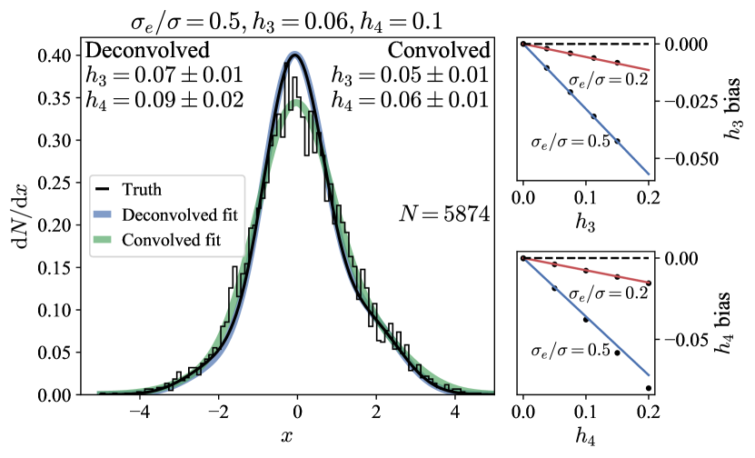
Figure 1: Gauss-Hermite series fitting to a mock distribution: the left panel shows a sample of $\displaystyle N$ draws (the black histogram) from a Gauss-Hermite series with $\displaystyle h_{3}=0.06$ and $\displaystyle h_{4}=0.1$ (the black line). The samples have then been scattered by an uncertainty of $\displaystyle 0.5$. The blue line is the fit result accounting for uncertainties whilst green is without accounting for uncertainties. Note that the recovered $\displaystyle h_{3}$ and $\displaystyle h_{4}$ are higher when the uncertainties are accounted for. This is also depicted in the right panels which show the bias in $\displaystyle h_{3}$ and $\displaystyle h_{4}$ as a function of these parameters if one fails to account for the uncertainties. Two choices of error are shown ($\displaystyle 0.2$ and $\displaystyle 0.5$). The lines give the approximations $\displaystyle h_{3}((1+(\sigma_{e}/\sigma)^{2})^{-3/2}-1)$ and $\displaystyle h_{4}((1+(\sigma_{e}/\sigma)^{2})^{-2}-1)$.

We have demonstrated how the Gauss-Hermite series can be used to model discrete data with heteroskedastic uncertainties, but only when the series is positive definite. Generically, for negative $\displaystyle h_{4}$ the series will produce negative wings making its use in a probabilistic framework awkward. In the next section, we will introduce a method to produce everywhere positive-definite pdfs which can be used as replacements for the Gauss-Hermite series.

3 A general family of weakly non-Gaussian pdfs

Our goal is to construct a family of everywhere positive pdfs, which can model weakly non-Gaussian distributions and also are able to incorporate observational uncertainties. This means that the models must have an easily computable convolution with a Gaussian kernel. This class of models is very desirable for modelling star-by-star data with heteroskedastic observational uncertainties, as otherwise the likelihood call for each star requires an integration over the uncertainty. We begin with a general scheme for constructing such models before discussing in detail two specific examples useful for modelling positive and negative excess kurtosis.

3.1 Model specification

With the requirement of analytic convolution with uncertainties, it is logical to investigate models which have been constructed by a convolution of a general kernel with a Gaussian. Further Gaussian kernel convolutions can then be simply performed and transform the models into another Gaussian convolution with a slightly modified general kernel. The models are

$$f(w)=b\int_{-\infty}^{\infty}\mathrm{d}y\,K(y)\alpha(y-b(w-w_{0})),$$ (14)

where $\displaystyle\alpha(y)$ is a unit Gaussian as defined in equation (2) and $\displaystyle K(y)$ is a general kernel normalized to have unit weight. $\displaystyle w_{0}$ and $\displaystyle b$ are parameters controlling the mean and variance of the model. To reproduce the unit Gaussian model $\displaystyle\alpha(w)$ when $\displaystyle K(y)=\delta(y)$, we require $\displaystyle b=1$ and $\displaystyle w_{0}=0$ in this limit, which implies $\displaystyle b$ and $\displaystyle w_{0}$ in general depend upon the parameters of the kernel $\displaystyle K(y)$. In the opposite limit where the kernel $\displaystyle K(y)$ is significantly broader than the unit Gaussian, $\displaystyle\alpha(y-b(w-w_{0}))\rightarrow\delta(y-b(w-w_{0}))$ so $\displaystyle f(w)\rightarrow bK(b(w-w_{0}))$, a scaled and shifted version of the kernel.

As with the Gauss-Hermite series, we have the freedom to introduce an arbitrary shift and scale to redefine the pdf in terms of $\displaystyle x=V+\sigma w$.

3.1.1 Model moments and cumulants

The moments of these models are given by

$$\begin{split}\mu_{n}(c)&=\int_{-\infty}^{\infty}\mathrm{d}w\,(w-c)^{n}f(w),\\ &=\frac{1}{b^{n}}\sum_{k=0}^{\lfloor\frac{n}{2}\rfloor}\binom{n}{2k}(2k-1)!!\tilde{\mu}_{n-2k}(bc-bw_{0}),\end{split}$$ (15)

where $\displaystyle\tilde{\mu}_{n}(c)$ are the moments of $\displaystyle K(y)$ (we use a tilde to denote properties of $\displaystyle K(y)$). For instance, the mean $\displaystyle\mu\equiv\mu_{1}(0)$ is given by

$$\mu=\frac{1}{b}\int_{-\infty}^{\infty}\mathrm{d}y\,yK(y-bw_{0})=\frac{\tilde{\mu}}{b}+w_{0},$$ (16)

where $\displaystyle\tilde{\mu}\equiv\tilde{\mu}(0)$. The central moments are defined as $\displaystyle\mu_{n}\equiv\mu_{n}(\mu)$, which can be combined in the usual way to find the cumulants. However, the cumulants $\displaystyle\kappa_{n}$ are more simply computed via the cumulant generating function $\displaystyle\ln\phi(u)$ defined as

$$\ln\phi(u)=\ln\int_{-\infty}^{\infty}\mathrm{d}w\,e^{iuw}f(w)=\sum_{r=1}^{r=\infty}\kappa_{r}\frac{(iu)^{r}}{r!}.$$ (17)

In this way, the $\displaystyle r$th cumulant is

$$\kappa_{r}=\frac{1}{i^{r}}\frac{\mathrm{d}^{r}\ln\phi(u)}{\mathrm{d}u^{r}}\Big{|}_{u=0}.$$ (18)

From the properties of the Fourier transform, the cumulant generating function of $\displaystyle f(w)$ is given by

$$\ln\phi(u)=iw_{0}u-\frac{u^{2}}{2b^{2}}+\ln\phi_{K}(u/b),$$ (19)

where $\displaystyle\phi_{K}(u)$ is the characteristic function of $\displaystyle K(y)$,

$$\phi_{K}(u)=\int_{-\infty}^{\infty}\mathrm{d}w\,e^{iuy}K(y).$$ (20)

From the cumulants, we define the variance $\displaystyle v\equiv\kappa_{2}$, the skewness $\displaystyle g\equiv\kappa_{3}/v^{3/2}$ and the excess kurtosis $\displaystyle\kappa\equiv\kappa_{4}/v^{2}$. We note that the variance of $\displaystyle K(y)$, $\displaystyle\tilde{v}$, is related to the variance of $\displaystyle f(w)$ by

$$v=\frac{1}{b^{2}}(\tilde{v}+1),$$ (21)

and all higher order cumulants ($\displaystyle r\geq 3$) satisfy $\displaystyle\kappa_{r}=\tilde{\kappa}_{r}/b^{r}$. This demonstrates that the signs of the skewness and the excess kurtosis of the kernel govern respectively the signs of the skewness and the excess kurtosis of the model.

3.1.2 Convolution with uncertainties

With such models, the convolution with observational uncertainties of magnitude $\displaystyle s$ is

$$\begin{split}f_{s}(w)&=\int_{-\infty}^{\infty}\mathrm{d}w^{\prime}f(w^{\prime})\mathcal{N}(w-w^{\prime}|s)\\ &=b\int_{-\infty}^{\infty}\mathrm{d}y\,K(ty)\alpha(y-b(w-w_{0})/t),\end{split}$$ (22)

where $\displaystyle t^{2}=1+b^{2}s^{2}$ and $\displaystyle f(w)$ is recovered for $\displaystyle t=1$ (i.e. $\displaystyle f_{0}(w)=f(w)$). In principle, if the convolution with $\displaystyle K(y)$ is analytic, the convolution with $\displaystyle K(ty)$ is likely to be analytic. As the convolution is a multiplication in Fourier space, the cumulant generating function of the error-convolved model is given by

$$\ln\phi_{s}(u)=\ln\phi(u)-\frac{u^{2}s^{2}}{2}.$$ (23)

3.1.3 Gauss-Hermite coefficients

The (unnormalized) Gauss-Hermite coefficients of this class of models are given by

$$h_{n}=\sqrt{4\pi}\int_{-\infty}^{\infty}\mathrm{d}w\,\alpha(w)H_{n}(w)f(w).$$ (24)

Note that in the limit where the kernel $\displaystyle K$ is significantly broader than the unit Gaussian, the Gauss-Hermite coefficients are given by

$$h_{n}\rightarrow\sqrt{4\pi}b\int_{-\infty}^{\infty}\mathrm{d}y\,K(b(y-w_{0}))\alpha(y)H_{n}(y),$$ (25)

i.e. they are the Gauss-Hermite coefficients of $\displaystyle K(b(y-w_{0}))$. A general expression for the Gauss-Hermite coefficients is found via the generating function of the Hermite polynomials given in equation (52). We compute the integral

$$\begin{split}\sum_{n=0}^{n=\infty}&\frac{z^{n}}{n!}\sqrt{n!}h_{n}=\sqrt{4\pi}b\,\times\\ &\int_{-\infty}^{\infty}\mathrm{d}y\,K(y)\int_{-\infty}^{\infty}\mathrm{d}w\,\alpha(y-b(w-w_{0}))\alpha(w)e^{\sqrt{2}wz-z^{2}/2}.\end{split}$$ (26)

Performing the $\displaystyle w$ integration leaves us with a single integral that is the same as the integral in equation (22) with $\displaystyle t^{2}=1+b^{2}$ i.e. $\displaystyle s=1$. We therefore can express $\displaystyle h_{n}$ in the compact form

$$h_{n}=\sqrt{4\pi}\sqrt{\frac{2^{n}}{n!}}\frac{\partial^{n}}{\partial z^{n}}\Big{[}e^{z^{2}/4}f_{1}(z)\Big{]}_{z=0}.$$ (27)

We conclude that if the error-convolved model has an analytic form, the Gauss-Hermite coefficients and error-deconvolved models can also be expressed analytically. The requirement $\displaystyle h_{1}=h_{2}=0$ is equivalent to $\displaystyle f_{1}(z)\sim e^{-z^{2}/4}(1+qz^{3})$ for small $\displaystyle z$ and constant $\displaystyle q$. To match the definition of $\displaystyle h_{n}$ given in equation (1), we normalize $\displaystyle h_{n}$ by $\displaystyle h_{0}=\sqrt{4\pi}f_{1}(0)$ such that the normalized $\displaystyle h_{0}=1$. All subsequent references to $\displaystyle h_{n}$ are to their normalized versions.

3.1.4 Model parametrization

There are two options for how to restrict the kernels (in particular, the parameters $\displaystyle b$ and $\displaystyle w_{0}$) when modelling: either we choose to fix the mean $\displaystyle\mu=0$ and variance $\displaystyle v=1$, or we fix $\displaystyle h_{1}=h_{2}=0$. The first option is analytically simpler as we have shown the moments of $\displaystyle f(w)$ are related to moments of $\displaystyle K(y)$. The latter option follows the parametrization of van der Marel & Franx (1993) who only consider non-zero $\displaystyle h_{n}$ for $\displaystyle n\geq 3$. In general, $\displaystyle h_{n}$ are complicated functions of the model parameters which do not have analytic roots, so we can only set $\displaystyle h_{1}=h_{2}=0$ approximately. We know the two options are equivalent for narrow kernels when $\displaystyle K(y)=\delta(y)$. In the wide $\displaystyle K(y)$ limit, we can use equation (25) to simplify the mathematics. Our general procedure for setting $\displaystyle h_{1}\approx h_{2}\approx 0$ is then stitching together the constant variance solution and the wide kernel solution. For symmetric kernels $\displaystyle K(y)$ ($\displaystyle\tilde{\mu}_{n}(0)=0$ for odd $\displaystyle n$) setting $\displaystyle w_{0}=0$ ensures $\displaystyle\mu=0$ and $\displaystyle h_{1}=0$ for all $\displaystyle b$.

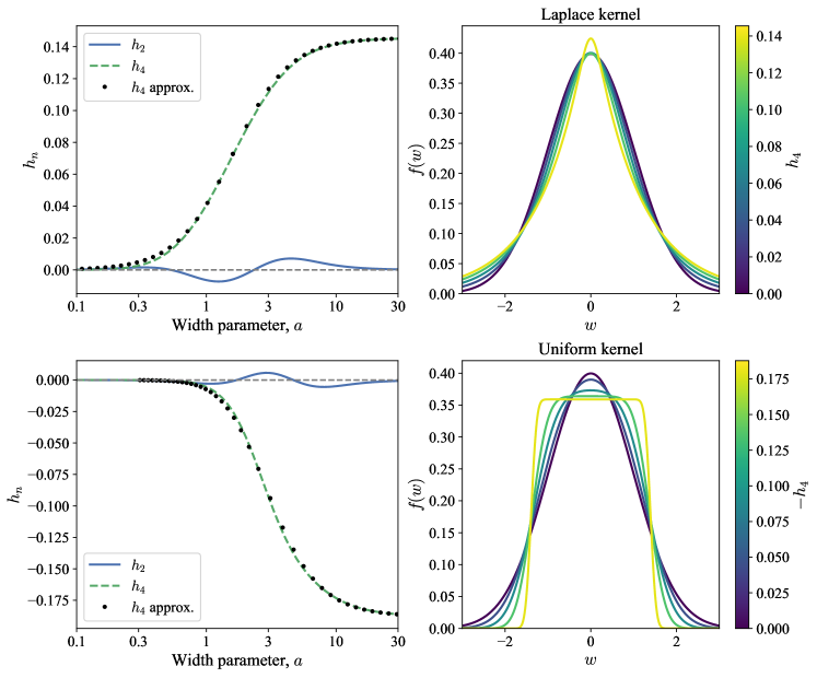
Figure 2: Our two families of pdfs with positive (top) and negative (bottom) excess kurtosis (setting skewness or $\displaystyle h_{3}$ to zero). The left panels show the 2nd (blue) and 4th (green) Gauss-Hermite coefficients of the models as a function of the model parameter, $\displaystyle a$. The model parameters have been selected to minimise variation of $\displaystyle h_{2}$. The right panels show the probability density functions in terms of the scaled coordinate $\displaystyle w=(x-V)/\sigma$ for different choices of $\displaystyle h_{4}$.

3.1.5 Half-kernels

The parity of the model $\displaystyle f(w)$ is equal to the parity of the kernel $\displaystyle K(y)$. We will find it useful to build arbitrary kernels from half-kernels

$$K(y)=\begin{cases}K_{+}(y)&y\geq 0\\ K_{-}(y)&y<0,\\ \end{cases}$$ (28)

such that $\displaystyle f(w)=f_{+}(w)+f_{-}(w)$. For a positive half-kernel $\displaystyle K_{+}(y)$, the corresponding negative half-kernel is given by $\displaystyle K_{-}(y)=K_{+}(-y)$. Therefore, by the symmetry properties of $\displaystyle f(w)$ and $\displaystyle K(y)$, we have $\displaystyle f_{-}(w)=f_{+}(-w)$. Additionally, the characteristic functions will satisfy the symmetry $\displaystyle\phi_{K-}(u)=\phi_{K+}(-u)$. In general, we can stitch together any two half-kernels to build a full kernel. This is a simple way to introduce skewness. There are two possibilities: either we ensure $\displaystyle K_{+}(0)=K_{-}(0)$ or $\displaystyle\int_{0}^{\infty}\mathrm{d}y\,K_{+}(y)=\int_{-\infty}^{0}\mathrm{d}y\,K_{-}(y)=\tfrac{1}{2}$. Here we use the latter choice.

4 Specific choices of kernel

With our general theory established, we now turn to some possible choices of kernel $\displaystyle K(y)$. We note here the similarity between our procedure and the method of Long & Murali (1992) for the construction of barred potentials via convolution with a kernel along the bar’s major axis. Williams & Evans (2017) and McGough et al. (2020) showed how flat-topped and cuspy barred potentials could be constructed by this method through convolution with a uniform and Laplace kernel respectively. Here we will follow those choices to construct two families of pdfs.

4.1 A negative excess kurtosis family – a uniform kernel

We first explore a simple symmetric kernel that produces a family of models with negative excess kurtosis. We later expand this model to incorporate skewness. As the models are symmetric $\displaystyle w_{0}=0$ satisfies both $\displaystyle\mu=0$ and $\displaystyle h_{1}=0$. Our choice for $\displaystyle K(y)$ is given by a top-hat function

$$K(y)=\begin{cases}\frac{1}{2a},&\mathrm{if}\,|y|<a,\\ 0,&\mathrm{otherwise},\end{cases}$$ (29)

for $\displaystyle a>0$, which has an error-convolved model given by

$$\begin{split}f_{s}(w)=\frac{b}{2a}\Big{[}\Phi\Big{(}\frac{bw+a}{t}\Big{)}-\Phi\Big{(}\frac{bw-a}{t}\Big{)}\Big{]},\end{split}$$ (30)

where $\displaystyle t^{2}=1+b^{2}s^{2}$ and $\displaystyle\Phi(x)$ is the cumulative distribution function for the unit Gaussian pdf:

$$\Phi(x)=\frac{1}{\sqrt{2\pi}}\int_{-\infty}^{x}\mathrm{d}t\,e^{-t^{2}/2}.$$ (31)

The model has zero mean, and the variance and excess kurtosis are given by

$$v=\frac{1}{b^{2}}\Big{(}1+\frac{a^{2}}{3}\Big{)},\quad\kappa=-\frac{2a^{4}}{15}\Big{(}1+\frac{a^{2}}{3}\Big{)}^{-2}.$$ (32)

We observe that there is a simple choice for $\displaystyle b$ such that the variance is unity: $\displaystyle b^{2}=(1+a^{2}/3)$.

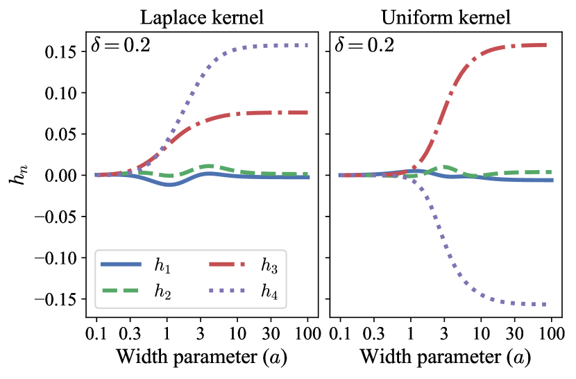
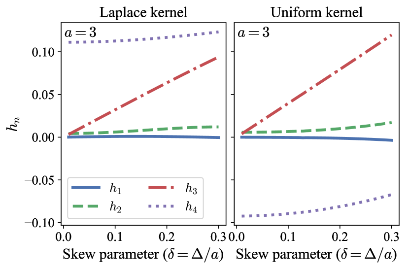
Figure 3: The Gauss-Hermite coefficients, $\displaystyle h_{n}$, for our two families of models. The left panels correspond to the positive excess kurtosis family with an Laplace kernel and the right to the negative excess kurtosis family with a uniform kernel. The top panels show the variation of $\displaystyle h_{n}$ with the width parameter $\displaystyle a$ (at fixed $\displaystyle\delta=0.2$) and the bottom variation of $\displaystyle h_{n}$ with the skewness parameter $\displaystyle\delta=\Delta/a$ (at fixed $\displaystyle a=3$). Note that $\displaystyle h_{1}\approx 0$ and $\displaystyle h_{2}\approx 0$ by design to mirror the Gauss-Hermite series from van der Marel & Franx (1993).

4.1.1 Fixing the Gauss-Hermite coefficients

We now turn to the selection of $\displaystyle b$ such that $\displaystyle h_{1}\approx h_{2}\approx 0$. As already highlighted, this cannot be done exactly and so only approximate expressions can be derived and choices of fitting functions must be made. For the uniform model, we explicitly detail the procedure we follow, which can be approximately followed for any other choice of model.

In the limit $\displaystyle a\rightarrow\infty$, we require $\displaystyle a/b\rightarrow k$ for constant $\displaystyle k$ such that the variance and $\displaystyle h_{2}$ remain finite. We introduce a general functional dependence of $\displaystyle b$ of the form

$$b^{2}=1+\Big{(}\frac{a}{k}\Big{)}^{2},$$ (33)

which encompasses the low (unity variance) and high $\displaystyle a$ limits for different choices of $\displaystyle k$. To recover the constant variance choice, we can set $\displaystyle k=k_{0}=\sqrt{3}$. Using equations (25) and (27), we determine the normalized $\displaystyle h_{2}$ and $\displaystyle h_{4}$ for large $\displaystyle a$ as

$$\begin{split}\lim_{\begin{subarray}{c}a\rightarrow\infty\\ a/b\rightarrow k\end{subarray}}h_{2}&=\sqrt{\frac{1}{2}}-\frac{2}{\sqrt{\pi}}ke^{-k^{2}/2}\Big{/}\mathrm{erf}\Big{(}\frac{k}{\sqrt{2}}\Big{)},\\ \lim_{\begin{subarray}{c}a\rightarrow\infty\\ a/b\rightarrow k\end{subarray}}h_{4}&=\sqrt{\frac{3}{8}}-\frac{2}{\sqrt{3\pi}}k^{3}e^{-k^{2}/2}\Big{/}\mathrm{erf}\Big{(}\frac{k}{\sqrt{2}}\Big{)}.\end{split}$$ (34)

We observe that there is a choice of $\displaystyle k=k_{\infty}$ which sets $\displaystyle\lim_{a\rightarrow\infty}h_{2}=0$ given by $\displaystyle k_{\infty}=1.399985\dots$, amazingly close to $\displaystyle 7/5$. With this choice, $\displaystyle\lim_{a\rightarrow\infty}h_{4}=-0.187777\dots\equiv h_{4,\infty}$. Therefore, to replicate the modelling with a Gauss-Hermite series which imposes the requirement that $\displaystyle h_{2}=0$ we can set $\displaystyle k=k_{\infty}$. This choice produces $\displaystyle|h_{2}|\lesssim 0.05$ everywhere. To improve this, we make $\displaystyle k$ a weak function of $\displaystyle a$ which reproduces the constant variance limit $\displaystyle k=k_{0}$ for small $\displaystyle a$ as

$$k(a)=k_{0}-(k_{0}-k_{\infty})\tanh(a/a_{0}),$$ (35)

where setting $\displaystyle a_{0}=3.3$ minimizes the variation of $\displaystyle h_{2}$ to $\displaystyle|h_{2}|\lesssim 0.006$. We show this set of models in the bottom panels of Fig. 2. We find that a good approximation for $\displaystyle a$ given $\displaystyle h_{4}$ is

$$a=a_{h4}\Big{(}\sqrt{\frac{h_{4,\infty}}{h_{4}}}-1\Big{)}^{-1/2},$$ (36)

where $\displaystyle a_{h4}=2$. This fitting function is shown in Fig. 2 . In this way, we can parameterize our models in terms of $\displaystyle h_{4}$.

Table 1: Key formulae for the two families of distributions introduced in this paper. $\displaystyle f_{s}(w)$ is the probability density function of the scaled and shifted coordinate $\displaystyle w=(x-V)/\sigma$ convolved with observational uncertainties $\displaystyle\sigma_{e}$ such that $\displaystyle s=\sigma_{e}/\sigma$. $\displaystyle\Phi(x)$ is the cumulative of the unit normal distribution. Further generic definitions are $\displaystyle w^{\prime}=w-w_{0}$, $\displaystyle t=1+b^{2}s^{2}$, $\displaystyle a_{+}=a+\Delta$, $\displaystyle a_{-}=a-\Delta$, $\displaystyle\delta=\Delta/a$, $\displaystyle b^{2}=1+(a/k)^{2}$ and $\displaystyle k=k_{0}-(k_{0}-k_{\infty})\tanh(a/a_{0})$. The parameters $\displaystyle a$, $\displaystyle b$ and $\displaystyle\Delta$ are chosen as per the ‘Auxiliary Functions’ and ‘Parameters’ columns to ensure $\displaystyle h_{1}\approx h_{2}\approx 0$ and to match a given $\displaystyle h_{3}$ and $\displaystyle h_{4}$. For a given $\displaystyle h_{3}$ and $\displaystyle h_{4}$, the quadratic for $\displaystyle\delta$ is solved, $\displaystyle a$ is computed using $\displaystyle h_{4,\mathrm{max}}(\delta)$ and finally $\displaystyle b$ and $\displaystyle w_{0}$ are found. Code for the computation of all formulae is provided at https://github.com/jls713/gh_alternative.

Name	$\displaystyle f_{s}(w)$	Auxiliary Functions	Parameters
			$\displaystyle h_{4,\infty}$	$\displaystyle a_{0}$	$\displaystyle a_{h3}$	$\displaystyle a_{h4}$	$\displaystyle k_{0}$	$\displaystyle k_{\infty,0}$
Uniform	$\displaystyle\!\begin{aligned} \frac{b}{2a_{+}a_{-}}\Big{[}a_{+}\Phi\Big{(}\frac{bw^{\prime}+a_{-}}{t}\Big{)}-a_{-}\Phi&\Big{(}\frac{bw^{\prime}-a_{+}}{t}\Big{)}\\ &-2\Delta\Phi\Big{(}\frac{bw^{\prime}}{t}\Big{)}\Big{]}\end{aligned}$	$\displaystyle\begin{array}[]{l}h_{4,\mathrm{max}}=(1-4.3\delta^{2})h_{4,\infty}\\ h_{3,\mathrm{max}}=0.82\delta\\ a=a_{hi}\Big{(}\sqrt{\frac{h_{i,\mathrm{max}}}{h_{i}}}-1\Big{)}^{-\tfrac{1}{2}}\\ k_{\infty}=k_{\infty,0}\sqrt{1+\delta^{2}+3\delta^{4}}\\ w_{0}=-\frac{\Delta}{2b}+\frac{\Delta}{3b}\tanh\Big{(}\frac{a}{a_{0}}\Big{)}\end{array}$	$\displaystyle-0.1878$	$\displaystyle 3.3$	$\displaystyle 2$	$\displaystyle 2$	$\displaystyle\sqrt{3}$	$\displaystyle\frac{7}{5}$
Laplace	$\displaystyle\!\begin{aligned} &\frac{b}{4a_{+}}\exp\Big{(}\frac{t^{2}-2a_{+}bw^{\prime}}{2a_{+}^{2}}\Big{)}\mathrm{erfc}\Big{(}\frac{t^{2}-a_{+}bw^{\prime}}{\sqrt{2}ta_{+}}\Big{)}\\ &+\frac{b}{4a_{-}}\exp\Big{(}\frac{t^{2}+2a_{-}bw^{\prime}}{2a_{-}^{2}}\Big{)}\mathrm{erfc}\Big{(}\frac{t^{2}+a_{-}bw^{\prime}}{\sqrt{2}ta_{-}}\Big{)}\end{aligned}$	$\displaystyle\begin{array}[]{l}h_{4,\mathrm{max}}=(1+2\delta^{2})h_{4,\infty}\\ h_{3,\mathrm{max}}=0.37\delta\\ a=a_{hi}\Big{(}\frac{h_{i,\mathrm{max}}}{h_{i}}-1\Big{)}^{-\tfrac{1}{2}}\\ k_{\infty}=k_{\infty,0}\sqrt{1+3\delta^{2}}\\ w_{0}=-\frac{\Delta}{b}+\frac{8\Delta}{7b}\tanh\Big{(}\frac{5a}{4a_{0}}\Big{)}\\ \end{array}$	$\displaystyle 0.1454$	$\displaystyle 2.25$	$\displaystyle 1.1$	$\displaystyle 1.6$	$\displaystyle\frac{1}{\sqrt{2}}$	$\displaystyle 1.08$

4.1.2 Incorporating skewness

Following the discussion in Section 3.1.5, a generalization of this model which incorporates some skewness is found by using a different uniform distribution for positive and negative $\displaystyle y$ as

$$K(y)=\begin{cases}\frac{1}{2a_{+}},&\mathrm{if}\,0<y<a_{+},\\ \frac{1}{2a_{-}},&\mathrm{if}\,-a_{-}<y<0,\\ 0,&\mathrm{otherwise},\end{cases}$$ (37)

for $\displaystyle a_{+}>0$ and $\displaystyle a_{-}>0$ which produces an error-convolved model of the form

$$\begin{split}f_{s}(w)=\frac{b}{2a_{+}a_{-}}\Big{[}a_{+}\Phi\Big{(}\frac{bw^{\prime}+a_{-}}{t}\Big{)}-a_{-}\Phi\Big{(}\frac{bw^{\prime}-a_{+}}{t}\Big{)}-2\Delta\Phi\Big{(}\frac{bw^{\prime}}{t}\Big{)}\Big{]},\end{split}$$ (38)

where $\displaystyle w^{\prime}=w-w_{0}$, $\displaystyle a=\tfrac{1}{2}(a_{+}+a_{-})$ and $\displaystyle\Delta=\tfrac{1}{2}(a_{+}-a_{-})<a$. We describe numerical calculation of $\displaystyle f_{s}(w)$ in Appendix F. In Table 4, we provide the cumulants for this model. As expected, $\displaystyle\Delta$ controls the skewness of the distribution, which we parametrize in a scale-free way using $\displaystyle\delta=\Delta/a$.

We use equation (25) to find expressions for $\displaystyle h_{1}$ and $\displaystyle h_{2}$ in the limit of large $\displaystyle a$ and $\displaystyle a/b=k$. Adopting the choice of $\displaystyle k$ for $\displaystyle\Delta=0$, $\displaystyle k=k_{\infty}=7/5$, we find $\displaystyle w_{0}\approx-\Delta/6b$ approximately sets $\displaystyle h_{1}=0$. We also find that $\displaystyle k_{\infty}$ must be made a function of $\displaystyle\delta=\Delta/a$ to retain $\displaystyle h_{2}=0$. With these choices, we set

$$\begin{split}k_{\infty}&=\frac{7}{5}\sqrt{1+\delta^{2}+3\delta^{4}},\\ w_{0}&=-\frac{\Delta}{2b}+\frac{\Delta}{3b}\tanh(a/a_{0}).\end{split}$$ (39)

where $\displaystyle\delta=\Delta/a$. We find that the maximum $\displaystyle|h_{4}|$ is $\displaystyle h_{4,\mathrm{max}}\approx(1-4.3\delta^{2})h_{4,\infty}$ and that the maximum $\displaystyle h_{3}$ is $\displaystyle|h_{3,\mathrm{max}}|\approx 0.82|\delta|$. We adopt the same functional form for $\displaystyle h_{3}(a)$ as $\displaystyle h_{4}(a)$, which means $\displaystyle h_{3}/h_{4}=h_{3,\mathrm{max}}/h_{4,\mathrm{max}}$. For a choice of $\displaystyle h_{3}$ and $\displaystyle h_{4}$, we first find $\displaystyle\delta$ by solving a quadratic. We then obtain $\displaystyle a$ from equation (36). The full set of parameters describing the model are given in Table 1.

In Fig. 3, we show the variation of $\displaystyle h_{n}$ for this model as a function of $\displaystyle a$ and $\displaystyle\delta$. We see how our choices have ensured $\displaystyle h_{1}\approx 0$ and $\displaystyle h_{2}\approx 0$. $\displaystyle\delta$ approximately controls $\displaystyle h_{3}$ at fixed $\displaystyle a$, and $\displaystyle a$ controls $\displaystyle h_{4}$ although there is some variation of $\displaystyle h_{4}$ with $\displaystyle\delta$.

4.2 A positive excess kurtosis family – a Laplace kernel

An extension to positive excess kurtosis can be constructed using a Laplace kernel. The exponential naturally produces broader tails than the Gaussian. The choice of kernel is

$$K(y)=\begin{cases}\frac{1}{2a_{+}}e^{-y/a_{+}},&\mathrm{if}\,y>0,\\ \frac{1}{2a_{-}}e^{y/a_{-}},&\mathrm{if}\,y<0,\end{cases}$$ (40)

for $\displaystyle a_{+}>0$ and $\displaystyle a_{-}>0$, which produces an error-convolved distribution of the form

$$\begin{split}f_{s}(w)&=\frac{b}{4a_{+}}\exp\Big{(}\frac{t^{2}-2a_{+}bw^{\prime}}{2a_{+}^{2}}\Big{)}\mathrm{erfc}\Big{(}\frac{t^{2}-a_{+}bw^{\prime}}{\sqrt{2}ta_{+}}\Big{)}\\ &+\frac{b}{4a_{-}}\exp\Big{(}\frac{t^{2}+2a_{-}bw^{\prime}}{2a_{-}^{2}}\Big{)}\mathrm{erfc}\Big{(}\frac{t^{2}+a_{-}bw^{\prime}}{\sqrt{2}ta_{-}}\Big{)},\end{split}$$ (41)

where $\displaystyle w^{\prime}=w-w_{0}$. This model is a sum of exponentially modified Gaussian distributions. Note that the products of exponentials and error functions require careful numerics when the arguments of the exponentials are large and positive. We discuss numerical implementation details in Appendix F.

In Table 4, we provide the cumulants for this model. We follow a similar procedure to the uniform kernel case for restricting the parameters $\displaystyle b$ and $\displaystyle w_{0}$ such that $\displaystyle h_{1}\approx h_{2}\approx 0$. One key difference is that our choice of parametrization of $\displaystyle h_{i}(a)$ is

$$a=a_{hi}\Big{(}\frac{h_{i,\mathrm{max}}}{h_{i}}-1\Big{)}^{-1/2},$$ (42)

with different scale parameters $\displaystyle a_{hi}$ for $\displaystyle h_{3}$ and $\displaystyle h_{4}$. We show the accuracy of this approximation in Fig. 2 along with the pdfs for $\displaystyle h_{3}=0$. The full model parametrization is given in Table 1.

In Fig. 3, we show the variation of $\displaystyle h_{n}$ for this model as a function of $\displaystyle a$ and $\displaystyle\delta$ alongside the equivalent for the uniform kernel. We see our choices have made $\displaystyle h_{1}\approx 0$ and $\displaystyle h_{2}\approx 0$. $\displaystyle h_{3}$ is controlled by $\displaystyle\delta$ at fixed $\displaystyle a$, and varying $\displaystyle a$ varies both $\displaystyle h_{3}$ and $\displaystyle h_{4}$ together.

4.3 Further choices of kernel

The general procedure we have employed for the uniform and Laplace kernels is applicable for a broader choice of kernels. The sole requirement is that the convolution of the kernel with a Gaussian is analytic. We have considered a number of other kernels with both positive and negative excess kurtosis. In Table 3, we detail a number of half-kernels $\displaystyle K_{+}(y)$ along with their corresponding error-convolved distributions $\displaystyle f_{s+}(w)$. Along with the uniform and Laplace kernels, we give expressions for a raised cosine distribution, a Gaussian distribution and a gamma distribution. In Table 4, we give the cumulants produced by stitching together two half-kernels with different scales ($\displaystyle a_{\pm}$). The raised cosine distribution produces a negative excess kurtosis family ($\displaystyle\kappa=-0.59$) and can be asymmetrized in the same way as the Laplace family. The Gaussian family produces a family of positive excess kurtosis but non-zero excess kurtosis is always accompanied by skewness. The gamma distribution, which is only defined for positive $\displaystyle y$, produces a positive excess kurtosis family. We note that the form of the models we have introduced encompasses the well-known Voigt profile which is formed from the convolution of a Cauchy distribution with a Gaussian. It is regularly used in spectroscopy, and can be computed using the real part of the Faddeeva function.

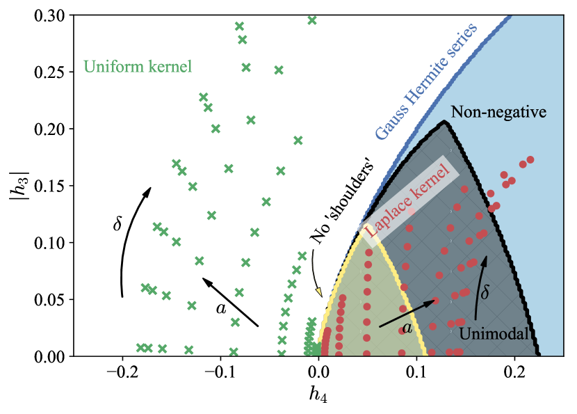
Figure 4: The space of Gauss-Hermite coefficients accessible by our new models: red points show the positive excess kurtosis family formed by the Laplace kernel whilst green crosses show the negative excess kurtosis family formed from the uniform kernel. The parameters $\displaystyle a$ and $\displaystyle\delta=\Delta/a$ act approximately like polar coordinates in this space. The points are spaced logarithmically in $\displaystyle a$ and linearly in $\displaystyle\delta$ (up to a maximum of $\displaystyle\delta=0.5$ as this is the range over which our approximations are valid). A Gauss-Hermite series can be constructed for all parts of the figure but only in the blue region are the series non-negative everywhere, only within the black hatched region are they unimodal and non-negative, and only within the yellow region do they have a fixed sign of the curvature in the tails.

4.4 Comparison with the Gauss-Hermite series

We close our investigation of the new families by comparison to the Gauss-Hermite series. In Fig. 4, we show the range of $\displaystyle h_{3}$ and $\displaystyle h_{4}$ accessible by our two families of models. We show for comparison the region of $\displaystyle(h_{3},h_{4})$ space in which the Gauss-Hermite series are non-negative, non-negative and unimodal, and non-negative, unimodal and with ‘no shoulders’ i.e. the sign of the curvature of the tails doesn’t change. In this space, the parameters $\displaystyle(a,\delta)$ behave approximately as polar coordinates. The regions of accessible $\displaystyle(h_{3},h_{4})$ form wedges highlighting a limitation of our models that the range of available $\displaystyle h_{3}$ depends upon $\displaystyle h_{4}$ and vice-versa. However, the same is true of the non-negative group of Gauss-Hermite models. The unimodal, non-negative Gauss-Hermite series essentially encompasses the range of models accessible by the Laplace kernel, which suggests the Gauss-Hermite is preferable for modelling positive excess kurtosis. However, the advantage of our new family is that non-negativity is built in and does not need to be checked numerically for each model. Additionally, all of our new positive excess kurtosis models have a constant sign for the curvature in the tails, whilst for smaller positive $\displaystyle h_{4}$ values than admitted by the new family the Gauss-Hermite can develop wings or shoulders.

In Fig. 5, we show the Gauss-Hermite series and the new family of models for four choices of $\displaystyle h_{3}$ and $\displaystyle h_{4}$. There is a great deal of similarity between the two different models although importantly the new models avoid the regions of negative probability for negative excess kurtosis. We also note that the new family of positive excess kurtosis models has stronger tails than the Gauss-Hermite series showing the presence of higher order Gauss-Hermite coefficients in their expansion. Another generic feature of our models that doesn’t appear to arise in the Gauss-Hermite series expansion is the presence of a ‘shoulder’ for skewed negative excess kurtosis models: a feature due to our method of stitching together half-kernels.

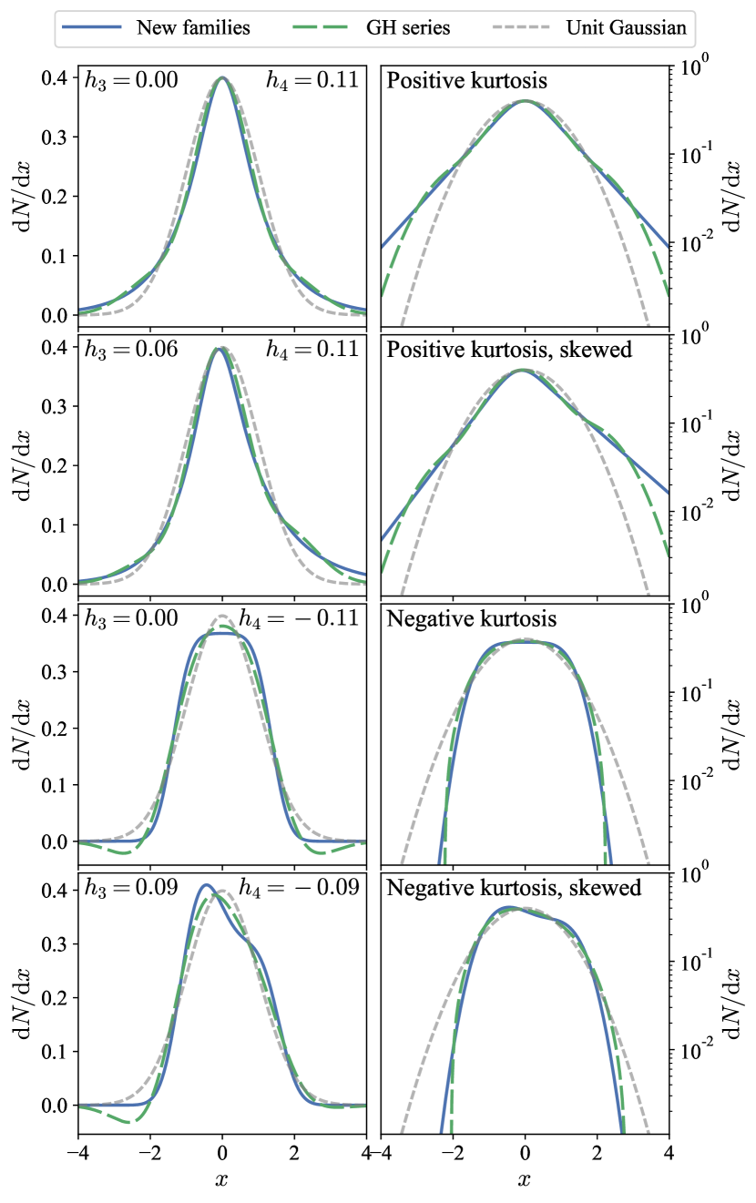
Figure 5: Comparison between the new models and the Gauss-Hermite series for four different choices of $\displaystyle h_{3}$ and $\displaystyle h_{4}$ (labelled in each row). Each set of panels show the new models in blue solid, the equivalent Gauss-Hermite series in green long-dashed and a reference unit Gaussian in light grey short-dashed. The left panels have a linear $\displaystyle y$ axis and right logarithmic. The Gauss-Hermite series models are normalized to have unit weight over the region of positivity. The two sets of models match well but for negative excess kurtosis the negative regions of the Gauss-Hermite series are avoided.

5 Application to dwarf spheroidal data

As an illustration of our approach, we will demonstrate its use on line-of-sight velocity data from dwarf spheroidal galaxies of the Milky Way. Dwarf spheroidal galaxies are gas-poor elliptical low stellar mass systems (Mateo, 1998). Within $\displaystyle\Lambda$ cold dark matter theory these objects are anticipated to be highly dark-matter dominated. This appears to be borne out by line-of-sight velocity measurements for the dwarf spheroidal galaxies of the Local Group and so make these objects ideal laboratories for investigating the properties of dark matter. The density profile of dark matter within these objects has received considerable attention, in particular the question of whether the central regions are cored or cuspy. The profile shape is a probe of both the effects of baryonic feedback on cold dark matter, or the properties of other dark matter candidates (such as self-interacting dark matter). However, pinning down the density profile is not a simple task due to the well-known mass-anisotropy degeneracy. Solutions to this include the use of proper motions (Massari et al., 2018) or performing analyses on different sub-populations within the dwarf spheroidals (Walker & Peñarrubia, 2011; Amorisco & Evans, 2012a). However, it has also been suggested that the velocity distribution contains sufficient information to break the mass-anisotropy degeneracy in its higher order moments, in particular the kurtosis (e.g. Łokas, 2002; Richardson & Fairbairn, 2013; Read et al., 2019). As highlighted by van der Marel & Franx (1993), kurtosis is a measure of orbital anisotropy with positive excess kurtosis associated with radial orbits. Here we will investigate how our new models can be used to constrain the higher order velocity moments from dwarf spheroidal data. We will focus on the specific example of the Fornax dSph as it has the largest line-of-sight velocity dataset.

5.1 Dynamical models of the Fornax dSph

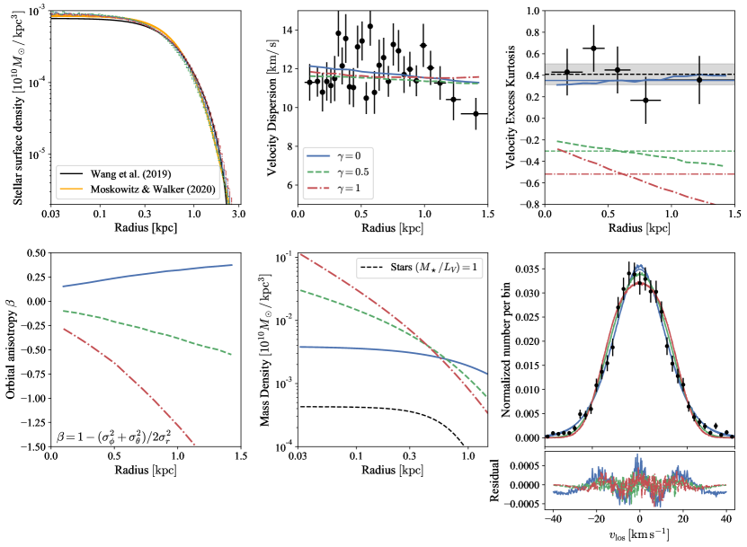
Figure 6: Dynamical models of the Fornax dwarf spheroidal galaxy. Data are always shown in black (statistics are weighted using membership probabilities from subsection 5.2, $\displaystyle x$ errorbars show the bin size and $\displaystyle y$ errorbars are from Poisson only, e.g. equation (6), so do not consider measurement uncertainties, although the dispersion is deconvolved by the median uncertainty) and the three models are blue solid (cored, $\displaystyle\gamma=0$), green dashed (weakly cusped, $\displaystyle\gamma=-0.5$) and red dash-dot (strongly cusped, $\displaystyle\gamma=-1$). The top left panel shows the density profiles as a function of radius. For the data, we always use the circularized radius $\displaystyle\sqrt{1-\epsilon}(x^{2}+y^{2}/(1-\epsilon)^{2})^{1/2}$ for flattening $\displaystyle\epsilon=0.31$ to compare to our spherical models. We also display the posterior distribution of the density fits to DES data from Moskowitz & Walker (2020) and the King fit to DES data from Wang et al. (2019) scaled to have $\displaystyle L_{V}=1.4\times 10^{7}\,L_{\odot}$ with $\displaystyle(M_{\star}/L_{V})=1$. The top middle panel shows the velocity dispersion and top right the excess kurtosis of the velocity distribution. The horizontal lines are the mean excess kurtosis of the models. The black band is the median and $\displaystyle\pm 1\sigma$ excess kurtosis of the model. In the bottom row we show the orbital anisotropy (left) and the mass density (middle) along with stellar density. In the bottom right, we show the model velocity distributions (binned histograms) along with fits using the pdfs in this work. The Fornax data are also shown. The models do an excellent job of capturing the kurtosis of the dynamical models, so much so that they are barely distinguishable in the upper panel, but the deviations are shown in the lower panel of residuals.

We take the spectroscopic sample of $\displaystyle 2633$ stars presented in Walker et al. (2009a), who provide line-of-sight velocities with uncertainties for all stars and a metallicity indicator, a pseudo-equivalent width measurement of the Mg triplet, along with its uncertainty for $\displaystyle 459$ stars. We convert the on-sky positions into projected circularized radius $\displaystyle R_{c}=\sqrt{1-\epsilon}(x^{2}+y^{2}/(1-\epsilon)^{2})^{1/2}$ where $\displaystyle x/y$ are the positions along the major/minor axis of Fornax with respect to the dwarf centre. We take the centre of Fornax as $\displaystyle(\alpha,\delta)=(2\mathrm{h}39\mathrm{m}53\mathrm{s},-34^{\circ}30^{\prime}32^{\prime\prime})$, the position angle as $\displaystyle 42.2\,\mathrm{deg}$ and the ellipticity of $\displaystyle\epsilon=0.31$ from the King profile fit of Wang et al. (2019). Some targets were observed multiple times by Walker et al. (2009a) from which an inverse-variance-weighted mean line-of-sight velocity and its error are estimated. For the remainder of the stars we use the single velocity measurement along with its error. Pascale et al. (2018) discuss the effect of undetected binarity on the Fornax velocity distributions by comparing samples with and without binaries as determined by repeat observations. They find the distributions are very similar (less than $\displaystyle 4\,\mathrm{per\,cent}$ probability the distributions are drawn from different samples) so we conclude binarity is unimportant and do not attempt to correct for it. We correct for the velocity gradient across the dwarf produced by perspective rotation from the bulk proper motion using the equations in Walker et al. (2008) and the proper motion measurements from Gaia Collaboration et al. (2018b).

In addition to the spectroscopic data, we use the Fornax surface density profile measurements from Dark Energy Survey Data from Wang et al. (2019) and Moskowitz & Walker (2020). Wang et al. (2019) provide a best-fitting King profile to the data although acknowledge all the analytic forms they consider do not exactly match the data. Moskowitz & Walker (2020) provide posterior draws from the parameters of a three-component Plummer-like profile, but with a steeper $\displaystyle\rho\propto r^{-9}$ fall-off. We assume a distance to Fornax of $\displaystyle 138\,\mathrm{kpc}$ (Mateo, 1998; Rizzi et al., 2007) although our results are not particularly sensitive to this choice.

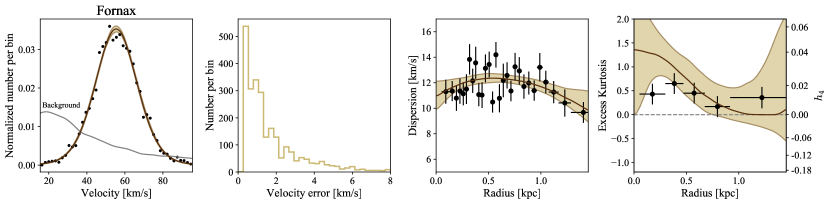
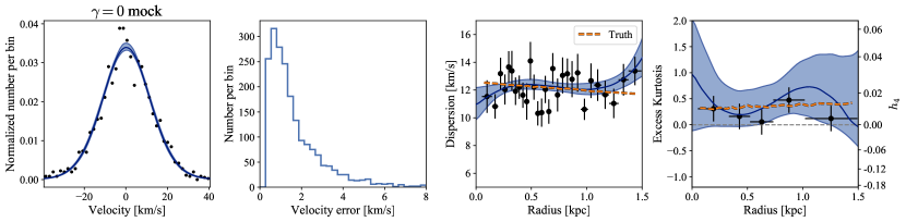
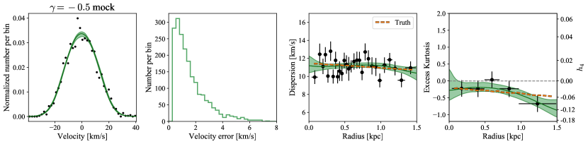
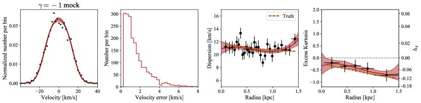
Figure 7: Fits of our family of pdfs to the Fornax data (top row) and three mock Fornax datasets (bottom three rows). The left column shows the velocity distribution of the data (mocks) in black and the median with $\displaystyle\pm 1\sigma$ fits of the models. In the top panel we also show the background Galaxia (Sharma et al., 2011) model used. The second column shows the distribution of uncertainties. The third and fourth columns show the (membership-weighted) dispersion and excess kurtosis data (black with errorbars showing the bin size in $\displaystyle x$ and Poisson errors in $\displaystyle y$) and fits along with the truth for the mocks in orange.

For constructing models of Fornax, we use the Agama dynamical modelling framework from Vasiliev (2019). Such an approach has also been taken by Pascale et al. (2018) in fitting density and velocity data on Fornax. To model the stellar distribution, we use the spheroidal distribution functions similar to those developed in work by Williams & Evans (2015) and Posti et al. (2015). They take the form

$$\begin{split}f(\boldsymbol{J})&=\frac{f_{0}}{(2\pi)^{3}}g(\boldsymbol{J})^{-\Gamma}\exp\bigg{[}-\left(\frac{g(\boldsymbol{J})}{J_{\mathrm{cutoff}}}\right)^{\zeta}\bigg{]},\\ g(\boldsymbol{J})&\equiv g_{r}J_{r}+\tfrac{1}{2}(3-g_{r})(J_{z}\,+|J_{\phi}|),\end{split}$$ (43)

The linear combination of the actions $\displaystyle g(\boldsymbol{J})$ is set to produce approximately spherical models and $\displaystyle g_{r}$ controls the degree of radial anisotropy. The models have an exponential cutoff at scale $\displaystyle J_{\mathrm{cutoff}}$ with the option of a flexible inner slope controlled by $\displaystyle\Gamma$. For the dark matter, we consider the simple family of density profiles

$$\rho_{\mathrm{DM}}(r)=\rho_{0}(r/r_{s})^{-\gamma}(1+r/r_{s})^{-3.2}.$$ (44)

For the potential from the stars, we fit the projection of a 3d power-law of the form $\displaystyle\rho_{\star,0}(1+(r/r_{\star})^{2})^{-9/2}$ to the Moskowitz & Walker (2020) density profile and assume a $\displaystyle V$-band stellar mass-to-light ratio of $\displaystyle 1$ and $\displaystyle L_{V}=1.4\times 10^{7}L_{\odot}$ (Irwin & Hatzidimitriou, 1995).

We use three values of the inner dark-matter density slope $\displaystyle\gamma=(0,0.5,1)$ and by-hand approximately match the density profile and the velocity dispersion profile of Fornax as shown in Fig. 6. The chosen parameters are given in Table 2. As our models are spherical, we always compare to the circularized radius $\displaystyle R_{c}$ distributions for the data. We also opt to weight the moments calculated from the data by membership probabilities computed in the next subsection and only consider stars within $\displaystyle 55\,\mathrm{km\,s}^{-1}$ of the mean velocity of Fornax (approximately $\displaystyle 5$ times the dispersion of Fornax).

Table 2: Parameters of our action-based Fornax models. The models differ primarily in their inner dark matter slope $\displaystyle\gamma$. $\displaystyle\rho_{0}$ and $\displaystyle r_{s}$ are the normalization and scale radius of the dark matter halo with units $\displaystyle 10^{10}M_{\odot}/\,\mathrm{kpc}^{3}$ and $\displaystyle\mathrm{kpc}$. $\displaystyle f_{0}$ is the normalization of the stellar distribution (with units $\displaystyle 10^{10}M_{\odot}/(\mathrm{kpc\,km\,s}^{-1})^{3-\Gamma}$). $\displaystyle\Gamma$ controls the central density slope of the stars, $\displaystyle J_{\mathrm{cutoff}}$ (with units $\displaystyle\mathrm{kpc\,km\,s}^{-1}$) and $\displaystyle\zeta$ govern the location and strength of the stellar exponential break, and $\displaystyle g_{r}$ the radial anisotropy of the stars.

$\displaystyle\gamma$	$\displaystyle\rho_{0}$	$\displaystyle r_{s}$	$\displaystyle f_{0}$	$\displaystyle\Gamma$	$\displaystyle J_{\mathrm{cutoff}}$	$\displaystyle g_{r}$	$\displaystyle\zeta$
$\displaystyle 0.0$	$\displaystyle 0.0039$	$\displaystyle 4.0$	$\displaystyle 2\times 10^{-5}$	$\displaystyle 0.0$	$\displaystyle 1.3$	$\displaystyle 1.2$	$\displaystyle 0.6$
$\displaystyle 0.5$	$\displaystyle 0.005$	$\displaystyle 1.3$	$\displaystyle 7.6\times 10^{-6}$	$\displaystyle 0.0$	$\displaystyle 3.2$	$\displaystyle 1.6$	$\displaystyle 0.8$
$\displaystyle 1.0$	$\displaystyle 0.0038$	$\displaystyle 1.0$	$\displaystyle 3\times 10^{-6}$	$\displaystyle 0.2$	$\displaystyle 8.6$	$\displaystyle 1.9$	$\displaystyle 1.4$

We observe that the three models have different anisotropy (the cuspy model is tangentially-biased whilst the cored model is more radially-biased) which correspond to differences in the excess kurtosis. Although all three models have very similar tracer density profiles and velocity dispersion profiles, the mass density distributions and hence anisotropy profiles are very different (e.g., Binney & Mamon, 1982; Evans et al., 2009). From this admittedly simplistic fitting approach, it seems the kurtosis of the data favours more cored models of Fornax, a conclusion also reached by others (Amorisco et al., 2013; Pascale et al., 2018; Read et al., 2019). However, this is sensitive to how one allocates membership of the dSph – for instance, Łokas (2009) and Amorisco & Evans (2012b) find negative excess kurtosis, possibly due to overly strict thresholds on membership, whilst Breddels & Helmi (2013) find the excess kurtosis is approximately zero.

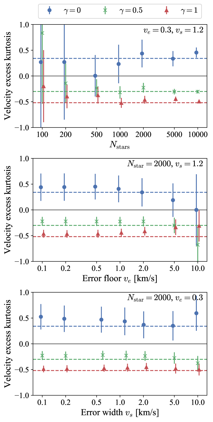
Figure 8: Measurement of velocity excess kurtosis using discrete samples of dynamical dwarf spheroidal models. Three models are inspected (cored = blue dot, weak cusp = green cross, strong cusp = red triangle). In the top panel the number of tracers is varied, central panel the line-of-sight velocity error floor is varied and bottom panel the width of the velocity error distribution varied. The dashed lines show the true values.

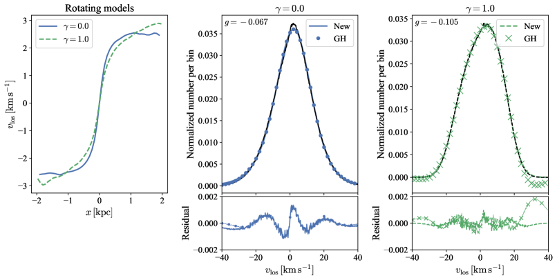
Figure 9: Example of rotating dynamical dwarf spheroidal models. Left panel shows the rotation curve of a cored (blue solid) and cuspy (green dashed) model. $\displaystyle x$ is the on-sky coordinate perpendicular to the rotation axis. The right two panels show the velocity distributions $\displaystyle\mathrm{sgn}(x)v_{\mathrm{los}}$ in black along with fits using the new models of this paper (lines) and the Gauss-Hermite series (with dots and crosses). The skewness $\displaystyle g$ is given in each panel.

5.2 Extracting kurtosis profiles

With our dynamical models for Fornax in place, we now wish to extract the kinematic properties as a function of location in the dwarf spheroidal given known uncertainties. For this we use the newly introduced models. For the data, we avoid applying arbitrary cuts to the data, and instead employ a mixture model for the dwarf plus background Milky Way contaminants. To incorporate more information on dwarf membership, we use the Mg triplet equivalent width measurements from Walker et al. (2009a) in addition to the velocities. When these measurements are unavailable we assign a default value with an uncertainty of $\displaystyle 1000\,$Å.

5.2.1 Chemo-kinematic mixture model

The likelihood for an individual star at (circularized) radius $\displaystyle R$ with velocity $\displaystyle(v\pm\sigma_{v})$ and equivalent width $\displaystyle(W\pm\sigma_{W})$ is

$$\begin{split}\mathcal{L}&(v,W|\sigma_{v},\sigma_{W},R)=\\ &p_{\mathrm{mem}}(R)f_{\sigma_{v}}(v|\mu(R),\sigma(R),h_{4}(R))\mathcal{N}(W-W_{\mathrm{d}}|\sqrt{\sigma_{W}^{2}+\sigma_{W\mathrm{d}}^{2}})\\ &+(1-p_{\mathrm{mem}}(R))B(v|\sigma_{v})\mathcal{N}(W-W_{\mathrm{o}}|\sqrt{\sigma_{W}^{2}+\sigma_{W\mathrm{o}}^{2}}),\end{split}$$ (45)

where $\displaystyle f_{\sigma_{v}}(v|\mu(R),\sigma(R),h_{4}(R))$ are the models introduced in this paper and the functions $\displaystyle\mu(R)$, $\displaystyle\sigma(R)$ and $\displaystyle h_{4}(R)$ are the parameters of the line-of-sight velocity distribution as a function of radius (mean, dispersion parameter and $\displaystyle h_{4}$). We assume $\displaystyle h_{3}=0$ everywhere. We use interpolating splines for $\displaystyle\mu(R)$, $\displaystyle\sigma(R)$ and $\displaystyle h_{4}(R)$ specifying $\displaystyle\mu_{k}$, $\displaystyle\sigma_{k}$ and $\displaystyle h_{4k}$ at 4 radii equally spaced in radius percentiles between the $\displaystyle 1$st and $\displaystyle 99$th of the data.

For the velocity distribution of the background Milky Way contaminants $\displaystyle B(v|\sigma_{v})$, we use Galaxia (Sharma et al., 2011) to sample stars in a $\displaystyle 8\,\mathrm{deg}^{2}$ field around Fornax and in the magnitude range $\displaystyle 18<V<20$. To convert the samples into a probability density function, we utilise a Gaussian kernel density estimate with a minimum kernel size of $\displaystyle 3\,\mathrm{km\,s}^{-1}$. For a range of uncertainties $\displaystyle\sigma_{v}$, we use a broader kernel of $\displaystyle\sqrt{(3\,\mathrm{km\,s}^{-1})^{2}+\sigma_{v}^{2}}$ and compute the velocity and uncertainty dependent background model $\displaystyle B(v|\sigma_{v})$ for each star. $\displaystyle\mathcal{N}(W-W_{i}|\sqrt{\sigma_{W}^{2}+\sigma_{Wi}^{2}})$ are Gaussians for the equivalent width measurements with free means $\displaystyle W_{i}$ and widths $\displaystyle\sigma_{Wi}$. The probability of membership $\displaystyle p_{\mathrm{mem}}$ is a function of on-sky location

$$p_{\mathrm{mem}}(R)=1-\frac{n_{\mathrm{b}}}{n_{\mathrm{b}}+n_{\mathrm{d}}\Sigma_{\mathrm{d}}(R)/\Sigma_{\mathrm{d}}(100\,\mathrm{pc})},$$ (46)

where $\displaystyle n_{\mathrm{b}}$ is the on-sky background density from Galaxia ($\displaystyle 0.23$ stars / arcmin²), $\displaystyle n_{\mathrm{d}}$ is a free parameter giving the on-sky dwarf central density and $\displaystyle\Sigma_{\mathrm{d}}(R)$ is the median normalized density profile from Moskowitz & Walker (2020).

We adopt uniform priors on $\displaystyle\mu_{k}$, $\displaystyle\ln\sigma_{k}$ and $\displaystyle h_{4k}$, where we work with a tanh transformation of $\displaystyle h_{4}$ to ensure it stays within the required range $\displaystyle-0.188<h_{4}<0.145$. For the equivalent-width models, we employ uniform priors for $\displaystyle W_{i}$ and $\displaystyle\ln\sigma_{Wi}$. We use a uniform prior for the logarithm of the dwarf number density, $\displaystyle\ln n_{\mathrm{d}}$. We therefore have a total of $\displaystyle 17$ parameters: $\displaystyle 3$ groups of $\displaystyle 4$ spline points $\displaystyle(\{\mu_{k}\},\{\ln\sigma_{k}\},\{h_{4k}\})$, $\displaystyle 2$ sets of equivalent-width mean and dispersion $\displaystyle(\{W_{i}\},\{\ln\sigma_{Wi}\})$ and the density $\displaystyle n_{\mathrm{d}}$. We sample from the product of the likelihood in equation (45) over stars using the emcee package (Foreman-Mackey et al., 2013). We focus on the results for $\displaystyle\sigma(R)$ and $\displaystyle h_{4}(R)$ below.

For the other parameters, we find the mean velocity of Fornax is $\displaystyle(55.3\pm 0.2)\,\mathrm{km\,s}^{-1}$ (computed by inverse-variance weighting of the spline points), consistent with that reported by McConnachie (2012). We find an indication of radial variation of the mean velocity with the central regions ($\displaystyle\lesssim 100\,\mathrm{pc}$) at a velocity $\displaystyle\sim 2\,\mathrm{km\,s}^{-1}$ higher. However, all spline points have consistent mean velocities within their uncertainties. We re-ran our models with a mean which doesn’t vary radially and find the conclusions on the variance and kurtosis profiles unchanged. As found by Walker et al. (2009b), Fornax stars are not well separated from the background stars in the Mg equivalent width measurement. For Fornax, we find $\displaystyle W_{\mathrm{d}}=(0.616^{+0.006}_{-0.006})$Å and $\displaystyle\sigma_{W\mathrm{d}}=(0.109^{+0.005}_{-0.005})$Å, whilst for the background distribution we find $\displaystyle W_{\mathrm{o}}=(0.52^{+0.12}_{-0.13})$Å and $\displaystyle\sigma_{W\mathrm{o}}=(0.34^{+0.11}_{-0.07})$Å. Finally, for the central density of Fornax we find $\displaystyle n_{\mathrm{d}}=(20.8^{+3.1}_{-2.5})$ stars$\displaystyle\,/\,\mathrm{arcmin}^{2}$. This number obviously depends on the magnitude selection of stars so it is more informative to compare relative to the background density, assumed to be $\displaystyle n_{\mathrm{b}}=0.23$ stars / arcmin². We find $\displaystyle n_{\mathrm{d}}/n_{\mathrm{b}}\approx 90$, in line with the results from Battaglia et al. (2006) (who find $\displaystyle n_{\mathrm{d}}/n_{\mathrm{b}}\approx(72/0.78)=93$) or Wang et al. (2019) (who find $\displaystyle n_{\mathrm{d}}/n_{\mathrm{b}}\approx 85$).

5.2.2 Results

The results of our procedure for the Fornax data are shown in the top panels of Fig. 7. In agreement with the simple weighted binned estimates (black points), we find that the data favours positive excess kurtosis models. The uncertainties are larger than the binned estimates as they also incorporate uncertainty from the measurement error and membership probabilities. We have also run our fitting using the Gauss-Hermite series for $\displaystyle h_{4}>0$ (where it is positive-definite). The results are shown in Fig. 11. The recovered $\displaystyle h_{4}$ profile is very similar to using the Laplace kernel (see Fig. 12) but the excess kurtosis is smaller, partly because the Gauss-Hermite series does not admit excess kurtosis larger than $\displaystyle\sim 0.5$.

To test our procedure, we also attempt to recover the kinematic profiles from our mock dynamical data. For this, we require an approximation to the uncertainty distribution, for which we use a gamma distribution $\displaystyle(\sigma_{v}-v_{e})/v_{s}\sim\Gamma(1.1,1)$. $\displaystyle v_{e}$ is an error floor and $\displaystyle v_{s}$ governs the width of the tail of the error distribution. We set $\displaystyle v_{e}=0.3\,\mathrm{km\,s}^{-1}$ and $\displaystyle v_{s}=1.2\,\mathrm{km\,s}^{-1}$, which gives a good match to the error distribution of the Fornax sample. From our mock dynamical models, we select $\displaystyle N_{\mathrm{stars}}=2000$ stars, assign uncertainties and scatter the velocities by the uncertainty. We do not use a background model and set $\displaystyle p_{\mathrm{mem}}=1$ for all mock data. We show the results of applying our modelling to the three models in the lower panels of Fig. 7. We find the recovery of the dispersion and excess kurtosis or $\displaystyle h_{4}$ is satisfactory.

We run further tests on the recovery of the excess kurtosis of our mock dynamical models with the quality and size of the dataset. For speed, we ignore the radial dependence of $\displaystyle\mu$, $\displaystyle\sigma$ and $\displaystyle h_{4}$. Additionally, we set a prior lower limit on $\displaystyle\sigma=0.05\,\mathrm{km\,s}^{-1}$. We run a set of three experiments varying (i) the number of stars $\displaystyle N_{\mathrm{stars}}$, (ii) the error floor, $\displaystyle v_{e}$, and (iii) the scale of the velocity error distribution, $\displaystyle v_{s}$. We use default parameters of $\displaystyle N_{\mathrm{star}}=2000$, $\displaystyle v_{s}=1.2\,\mathrm{km\,s}^{-1}$ and $\displaystyle v_{e}=0.3\,\mathrm{km\,s}^{-1}$ as used in the previous test. We use a fixed random seed to generate the mock samples from the models. The results of these experiments are shown in Fig. 8. We have varied $\displaystyle N_{\mathrm{star}}$ from $\displaystyle 100$ to $\displaystyle 10000$ and find that significant negative excess kurtosis can be found with relatively few stars ($\displaystyle\approx 200$), but for a significant positive excess kurtosis measurement we require $\displaystyle\gtrsim 2000$ stars. We have varied the error floor from $\displaystyle v_{e}=0.1$ up to $\displaystyle v_{e}=10\,\mathrm{km\,s}^{-1}$ finding that only for $\displaystyle v_{e}\lesssim 2\,\mathrm{km\,s}^{-1}$ can the sign of the excess kurtosis be reliable determined, although again negative excess kurtosis is detectable for $\displaystyle v_{e}\sim 5\,\mathrm{km\,s}^{-1}$. Finally, we have varied $\displaystyle v_{s}$ from $\displaystyle 0.1$ to $\displaystyle 10\,\mathrm{km\,s}^{-1}$ finding its effect on the recovery and size of the uncertainties to be quite weak such that for all of our tests we can fairly reliably distinguish the sign of the excess kurtosis and for $\displaystyle v_{s}\lesssim 2\,\mathrm{km\,s}^{-1}$ the models are distinguishable. Although our results are tailored for Fornax, they can be extended to other dwarf spheroidals by scaling by the dispersion of Fornax of $\displaystyle 11\,\mathrm{km\,s}^{-1}$.

5.3 Extension to rotation

To conclude our investigation into the use of the new models in the modelling of dwarf spheroidal data, we briefly demonstrate their application to rotating galaxies. Typically dwarf spheroidals exhibit negligible rotation and most detected rotation can be attributed to perspective effects from the projection of the bulk proper motion (Walker et al., 2008; Amorisco & Evans, 2012b). However, if rotation is present, the combined signals of shift in the mean velocity and skewness may prove powerful for its separation from perspective rotation (Amorisco & Evans, 2012b).

We modify the dynamical models by multiplying by an odd function of the $\displaystyle z$-component of angular momentum, $\displaystyle J_{\phi}$,

$$f_{\mathrm{rot}}(\boldsymbol{J})=f(\boldsymbol{J})\Big{(}1+k\,\mathrm{sgn}(J_{\phi})\Big{)}.$$ (47)

$\displaystyle k$ controls the degree of rotation and can take values $\displaystyle|k|\leq 1$. We investigate the cored $\displaystyle\gamma=0$ and cusped $\displaystyle\gamma=1$ models from the previous section. We choose $\displaystyle k=0.3$ for the cored model and $\displaystyle k=0.2$ for the cusped model, and view the models perpendicular to the rotation axis.

In Fig. 9, we show the rotation curves of the two models. The rotation reaches $\displaystyle\sim 3\,\mathrm{km\,s}$ for both models. Such a large rotation signal in Fornax would be obvious so this experiment is purely illustrative. We also display the line-of-sight velocity distributions (where the symmetry allows us to increase the number statistics by multiplying the velocities by the sign of $\displaystyle x$). We see both distributions are weakly skewed ($\displaystyle g=-0.067$ for the cored model and $\displaystyle g=-0.105$ for the cusped). Both the Gauss-Hermite series and the new models from this paper provide excellent fits to the distributions. In the case of the positive excess kurtosis model the fits are near identical. However, we see for the cusped negative excess kurtosis model the residuals with respect to our new models are in general smaller and in particular better capture the right-hand wing.

6 Application to spectral fitting

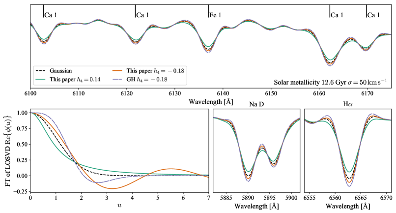
Figure 10: Single stellar population (solar metallicity, $\displaystyle 12.6\,\mathrm{Gyr}$ convolved with different choices of line-of-sight velocity distribution (LOSVD). Four LOSVDs are used, all with identical $\displaystyle\sigma=50\,\mathrm{km\,s}^{-1}$ parameters (which does not equal the velocity dispersion except for the Gaussian): (i) Gaussian in black dashed, (ii) solid green this paper’s model $\displaystyle h_{4}=0.14$, (iii) solid orange this paper’s model $\displaystyle h_{4}=-0.18$ and (iv) Gauss-Hermite series with $\displaystyle h_{4}=-0.18$. The top panel and bottom right two panels show example regions of the spectra. The corresponding Fourier transforms of the LOSVDs (important in the computation of the spectra) are given in the bottom left. Note the selected $\displaystyle h_{4}$ parameters are extreme to exaggerate the effects.

As discussed in Section 2, the Gauss-Hermite series was originally introduced for the extraction of kinematics from spectra (Gerhard, 1993; van der Marel & Franx, 1993). Given a library of single stellar population spectra, Cappellari & Emsellem (2004) describe a penalized likelihood algorithm for the simultaneous extraction of the age-metallicity properties of a measured galaxy and the kinematics via the convolution of the library with a Gauss-Hermite series for the LOSVD. Cappellari (2017) showed how undersampling the LOSVD when the LOSVD dispersion is smaller than half the pixel spacing is problematic for accurate recovery of the kinematics (particularly the mean) but could be circumvented using the analytic Fourier transform of the Gauss-Hermite series. This is now the standard method in the spectral fitting code ppxf (Cappellari & Emsellem, 2004; Cappellari, 2017).

Although in the spectral fitting application the issue of negative wings in the LOSVD is less severe than in the application to discrete data, it still gives rise to unphysical features that could bias the recovery of kinematics. However, the new families of models introduced in this paper provide simple replacements for the Gauss-Hermite series in the spectral fitting procedure. This is because they too have analytic Fourier transforms. In fact, the Fourier transforms are simpler to evaluate than the real-space forms. The Fourier transforms for the two models are

$$\phi_{s}(u)=\frac{1}{2}e^{iw_{0}u-u^{2}t^{2}/2b^{2}}\Big{[}\frac{1}{1-ia_{+}u/b}+\frac{1}{1+ia_{-}u/b}\Big{]},$$ (48)

for the Laplace kernel, and

$$\phi_{s}(u)=\frac{1}{2}e^{iw_{0}u-u^{2}t^{2}/2b^{2}}\Big{[}\frac{e^{ia_{+}u/b}}{ia_{+}u/b}-\frac{e^{ia_{-}u/b}}{ia_{-}u/b}\Big{]},$$ (49)

for the uniform kernel. We have implemented the models within a version of the ppxf code and find that for the included examples the recovery of the kinematics is very similar to using a Gauss-Hermite series.

In Fig. 10, we show examples of a single stellar population with solar metallicity and of age $\displaystyle 12.6\,\mathrm{Gyr}$ (Vazdekis et al., 2010) convolved with different choices of LOSVD. For all models, we fix the parameter $\displaystyle\sigma=50\,\mathrm{km\,s}^{-1}$ but this does not mean the variance of all models are the same. We see that for $\displaystyle h_{4}>0$ the wings of the lines are broader than Gaussian and for $\displaystyle h_{4}<0$ they are narrower. We observe that when using the Gauss-Hermite series there are prominent bumps in the wings of the lines (particularly visible for H$\displaystyle\alpha$) due to the negative LOSVD but these are avoided when using the models of this paper. It should be noted however that in general the effects and differences are small and the large values of $\displaystyle|h_{4}|$ chosen for the example have been selected to exaggerate the effect. We also display the Fourier transform of the LOSVD. One feature of the Gauss-Hermite series is that it decays like $\displaystyle e^{-u^{2}}$ in Fourier space whereas our negative models oscillate and decay like $\displaystyle 1/u$. However, this is unimportant as the template spectra are bandwidth-limited and Nyquist-sampled so we only require the Fourier transform on a fixed grid ($\displaystyle u/\sigma<\pi$) and its behaviour for large $\displaystyle u$ is irrelevant. The only disadvantages to our suggested modifications are: (i) one cannot incorporate higher order moments $\displaystyle h_{5}$ or $\displaystyle h_{6}$ – these are already non-zero for our models. In practice, one rarely uses these higher order moments anyway; (ii) there is only a finite range of $\displaystyle h_{3}$ and $\displaystyle h_{4}$ accessible by our models. Already $\displaystyle h_{3}$ and $\displaystyle h_{4}$ are bounded in ppxf (default is between $\displaystyle-0.3$ and $\displaystyle 0.3$) but the difficulty with our models is in the inter-dependence of maximum $\displaystyle h_{3}$ and $\displaystyle h_{4}$ as shown in Fig. 4. One could use $\displaystyle a$ and $\displaystyle\delta$ as parameters instead.

7 Conclusions

We have introduced a new method for constructing probability distribution functions for the modelling of discrete stellar velocity data drawn from weakly non-Gaussian distributions and with heteroskedastic uncertainties. Our study was motivated by the limitation of the commonly used Gauss-Hermite series expansion. Although the Gauss-Hermite series has attractive properties for convolution with measurement uncertainty, a key limitation is that the Gauss-Hermite series does not give well-defined probability density functions – there are regions of negativity particularly for negative excess kurtosis models.

We have demonstrated a generic method for constructing everywhere positive families of probability functions through the convolution of a Gaussian with a choice of kernel. The resulting probability distribution function inherits the properties (moments and cumulants) of the kernel. We have examined in detail two choices of kernel, Laplace and uniform, which give rise to positive and negative excess kurtosis respectively and can be asymmetrised to incorporate skewness. Inspired by the standard implementation of the Gauss-Hermite expansion, we have restricted the models to have approximately $\displaystyle h_{1}=h_{2}=0$ such that the models can be used as a direct replacement for the Gauss-Hermite series. However, in theory, the models can be used in greater generality. We provide code for the evaluation of our models at https://github.com/jls713/gh_alternative.

We have demonstrated the use of our new models with two simple applications. The first is to discrete sets of line-of-sight velocity data in galactic modelling. We have shown through a series of dynamical models how non-Gaussianity can break mass-anisotropy degeneracies and how our methods allow for a flexible measurement of the excess kurtosis. This has a ready application to the dwarf galaxies around the Milky Way, for which large datasets of velocities of bright giant stars exist and for which the structure of the dark halo is an open question. For the specific example of the Fornax dwarf spheroidal galaxy, we have shown using a chemo-kinematical mixture model that the data seem to favour positive excess kurtosis velocity distributions and hence indicate cored dark matter density profiles. Additionally, we have tested our modelling procedure on a series of dynamical dwarf spheroidal galaxy models with varying dark matter profiles, finding good recovery of the kinematic profiles and that a cored model well reproduces the observed data. Furthermore, we have investigated how the excess kurtosis measurement depends on the number and uncertainty distribution of stellar tracers. For a Fornax-like dSph. $\displaystyle\gtrsim 2000$ stars with uncertainties $\displaystyle\lesssim 2\,\mathrm{km\,s}^{-1}$ are sufficient to measure the sign of the excess kurtosis and measure the mass density slope, although this assumes perfect knowledge of dwarf spheroidal membership. We have also shown how our models are able to capture skewness, which could be a powerful indicator of the subtle effects of rotation and immune to the effects of perspective.

Secondly, although our models were not motivated by spectral fitting applications, their analytic Fourier transforms allow them to be used in spectral fitting algorithms where they could reduce bias produced by negative wings in the line-of-sight velocity distributions of high quality data.

Our methods for characterising mildly non-Gaussian velocity distributions are flexible and adaptable, offering significant advantages over the conventional Gauss-Hermite series. The skewness and kurtosis of such distributions contain important clues on the orbits of the tracers and the gravitational potential in which they move. The sizes of such discrete velocity datasets – whether for populations in the Milky Way or its dwarf satellite entourage or for populations in external galaxies like globular clusters and planetary nebulae – have substantially increased in recent years. We envisage that our new methods will play an important role in exploiting these datasets to the full.

Data availability

All data used in this article are in the public domain: Walker et al. (2009a), Vazdekis et al. (2010), Gaia Collaboration et al. (2018b), Wang et al. (2019) and Moskowitz & Walker (2020).

Appendix A Hermite polynomials

The convention for the Hermite polynomials employed here follows van der Marel & Franx (1993) such that they are given by the relation

$$\Big{(}-\frac{\mathrm{d}}{\mathrm{d}y}\Big{)}^{l}\alpha(y)=\sqrt{l!}H_{l}(y/\sqrt{2})\alpha(y).$$ (50)

This is different from the standard $\displaystyle H_{n}(y)$ defined in e.g. Olver et al. (2016) which are given by $\displaystyle\sqrt{l!2^{l}}H_{l}(y)$. The first five Hermite polynomials are

$$\begin{split}H_{0}(y)&=1,\>\>H_{1}(y)=\sqrt{2}y,\>\>H_{2}(y)=\frac{1}{\sqrt{2}}(2y^{2}-1),\\ H_{3}(y)&=\frac{1}{\sqrt{6}}(2\sqrt{2}y^{3}-3\sqrt{2}y),\>\>H_{4}(y)=\frac{1}{\sqrt{24}}(4y^{4}-12y^{2}+3).\\ \end{split}$$ (51)

The generating function for this definition of the Hermite polynomials is given by

$$\sum_{n=0}^{n=\infty}\frac{z^{n}}{n!}\sqrt{n!}H_{n}(y)=e^{\sqrt{2}yz-z^{2}/2},$$ (52)

from which the $\displaystyle n$th polynomial can be found as

$$H_{n}(y)=\frac{1}{\sqrt{n!}}\frac{\partial^{n}}{\partial z^{n}}\Big{(}e^{\sqrt{2}yz-z^{2}/2}\Big{)}\Big{|}_{z=0}.$$ (53)

Appendix B Cumulants of the Gauss-Hermite series

The cumulant generating function of the Gauss-Hermite series given in equation (1) is given by

$$\begin{split}\ln\phi_{\mathrm{GH}}(u)&=\ln\int_{-\infty}^{\infty}\mathrm{d}x\,e^{iux}f(x)=\sum_{r=1}\kappa_{r}\frac{(iu)^{r}}{r!},\\ &=iVu-\frac{(\sigma u)^{2}}{2}+\ln\Big{[}1+\sum_{n\geq 3}i^{n}h_{n}H_{n}(\sigma u)\Big{]}.\end{split}$$ (54)

The cumulants are then given by

$$\begin{split}\kappa_{1}&=V+\tilde{\kappa}_{1},\>\>\kappa_{2}=\sigma^{2}+\tilde{\kappa}_{2},\>\>\kappa_{i}=\tilde{\kappa}_{i},\quad i\geq 3,\\ \tilde{\kappa}_{r}&=\sigma^{r}\frac{\mathrm{d}^{r-1}}{\mathrm{d}u^{r-1}}\Big{[}\Big{(}1+\sum_{n\geq 3}i^{n}h_{n}H_{n}(u)\Big{)}^{-1}\sum_{n\geq 3}i^{n-r}h_{n}\frac{\mathrm{d}H_{n}(u)}{\mathrm{d}u}\Big{]}_{u=0}.\end{split}$$ (55)

Performing the derivative produces long-winded expressions. For their evaluation, we require the Hermite numbers $\displaystyle H_{n}(0)$ given by

$$H_{n}(0)=(-1)^{n/2}\frac{\sqrt{n!}}{(n/2)!\sqrt{2^{n}}},$$ (56)

for even $\displaystyle n$ and zero for odd $\displaystyle n$, and the $\displaystyle n$th derivative of the Hermite polynomials is

$$\frac{\mathrm{d}^{r}H_{n}(x)}{\mathrm{d}x^{r}}\Big{|}_{x=0}=\sqrt{\frac{2^{r}n!}{(n-r)!}}H_{n-r}(0)=(-1)^{(n-r)/2}\frac{2^{r-n/2}\sqrt{n!}}{((n-r)/2)!},$$ (57)

for even $\displaystyle n-r$ and zero otherwise. Restricting to $\displaystyle h_{n}=0$ for $\displaystyle n>4$, we find for the first four cumulants (note all $\displaystyle\kappa_{r}$ are non-zero)

$$\begin{split}\kappa_{1}&=V+\sqrt{3}\sigma\lambda h_{3}\approx V+\sqrt{3}\sigma h_{3},\\ \kappa_{2}&=\sigma^{2}+\sigma^{2}\lambda^{2}(h_{4}(2\sqrt{6}+3h_{4})-3h_{3}^{2})\approx\sigma^{2}(1+2\sqrt{6}h_{4}),\\ \kappa_{3}&=\tfrac{1}{2}h_{3}\sigma^{3}\lambda^{3}\Big{(}8\sqrt{3}+12\sqrt{3}h_{3}^{2}-3h_{4}(8\sqrt{2}+5\sqrt{3}h_{4})\Big{)}\approx 4\sqrt{3}h_{3}\sigma^{3},\\ \kappa_{4}&=\tfrac{1}{2}\sigma^{4}\lambda^{4}\Big{(}16\sqrt{6}h_{4}-9h_{4}^{2}(8+6\sqrt{6}h_{4}+5h_{4}^{2})\\ &+12h_{3}^{2}(15h_{4}^{2}+8\sqrt{6}h_{4}-8)-108h_{3}^{4}\Big{)}\approx 8\sqrt{6}h_{4}\sigma^{4},\end{split}$$ (58)

where $\displaystyle\lambda=\Big{(}1+\sqrt{3/8}h_{4}\Big{)}^{-1}$ and the approximations for small $\displaystyle h_{n}$ agree with van der Marel & Franx (1993). Note that for larger values $\displaystyle|h_{4}|$, the excess kurtosis $\displaystyle\kappa=\kappa_{4}/\kappa_{2}^{2}$ is not a monotonic function of $\displaystyle h_{4}$.

Appendix C Convolution of a Gauss-Hermite series with Gaussian errors

In this appendix, we compute the convolution of a Gauss-Hermite series $\displaystyle f(x)$ with a Gaussian uncertainty distribution $\displaystyle\mathcal{N}(x-x^{\prime}|\sigma_{e})$ as

$$f_{\sigma_{e}}(x)=\int_{-\infty}^{\infty}\mathrm{d}x^{\prime}\,f(x^{\prime})\mathcal{N}(x-x^{\prime}|\sigma_{e}).$$ (59)

We work in terms of the scaled and shifted coordinate $\displaystyle w=(x-V)/\sigma$. Dropping the constant factors, we require the convolution

$$f_{s}(w)=\int_{-\infty}^{\infty}\mathrm{d}w^{\prime}\,f(w^{\prime})\mathcal{N}(w-w^{\prime}|s),$$ (60)

where

$$\mathcal{N}(w|s)=\frac{1}{\sqrt{2\pi s^{2}}}e^{-\tfrac{1}{2}w^{2}/s^{2}},$$ (61)

and $\displaystyle s=\sigma_{e}/\sigma$. For this computation, we shift to Fourier space. One attractive property of the Gauss-Hermite series is that the terms are eigenfunctions of the Fourier transform, $\displaystyle F$,

$$F\Big{\{}\alpha(w)H_{n}(w)\Big{\}}\equiv\int_{-\infty}^{\infty}\mathrm{d}w\,\alpha(w)H_{n}(w)e^{ikw}=\sqrt{2\pi}i^{n}H_{n}(k)\alpha(k).$$ (62)

Cappellari (2017) uses this property to rapidly convolve a model spectrum with the Gauss-Hermite series. Each term in the convolution of $\displaystyle\mathcal{N}(w|s)$ with $\displaystyle f(w)$ is given by

$$\mathcal{C}_{n}(w|s)\equiv\int\mathrm{d}w^{\prime}H_{n}(w^{\prime})\alpha(w^{\prime})\mathcal{N}(w-w^{\prime}|s).$$ (63)

Taking the Fourier transform of the convolution yields

$$F\Big{\{}\mathcal{C}_{n}(w|s)\Big{\}}=\sqrt{2\pi}i^{n}H_{n}(k)\alpha(k)e^{-s^{2}k^{2}/2}=\sqrt{2\pi}i^{n}H_{n}(k)\alpha(s^{\prime}k),$$ (64)

where $\displaystyle s^{\prime}=\sqrt{1+s^{2}}$. The inverse Fourier transform is given by

$$\mathcal{C}_{n}(w|s)=\frac{i^{n}}{\sqrt{2\pi}s^{\prime}}\int\mathrm{d}k^{\prime}e^{-ik^{\prime}\frac{w}{s^{\prime}}}H_{n}\Big{(}\frac{k^{\prime}}{s^{\prime}}\Big{)}\alpha(k^{\prime}).$$ (65)

The Hermite polynomials satisfy the following multiplication theorem (Eq. 18.18.13, Olver et al., 2016)

$$H_{n}(\gamma x)=\gamma^{n}\sum_{j=0}^{\lfloor\frac{n}{2}\rfloor}(1-\gamma^{-2})^{j}\frac{\sqrt{n!}}{j!2^{j}\sqrt{(n-2j)!}}H_{n-2j}(x).$$ (66)

Rewriting $\displaystyle H(k^{\prime}/s^{\prime})$ using this series and using the eigenfunction of the Fourier transform property of $\displaystyle H(k^{\prime})\alpha(k^{\prime})$ gives an expression for the convolution of each term as

$$\mathcal{C}_{n}(w|s)=\frac{\mathcal{N}(w|s^{\prime})}{s^{\prime n}}\sum_{j=0}^{\lfloor\frac{n}{2}\rfloor}s^{2j}\frac{\sqrt{n!}}{j!2^{j}\sqrt{(n-2j)!}}H_{n-2j}\Big{(}\frac{w}{s^{\prime}}\Big{)}.$$ (67)

The sum can be recombined into a single Hermite polynomial as

$$\mathcal{C}_{n}(w|s)=\frac{\mathcal{N}(w|s^{\prime})}{s^{\prime n}}(1-s^{2})^{n/2}H_{n}\Big{(}\frac{w}{\sqrt{1-s^{4}}}\Big{)}.$$ (68)

This formula can be derived directly from equation (63) using equation (7.374.8) of Gradshteyn & Ryzhik (2007). Note that the formula is valid for $\displaystyle s>1$ although it requires numerical care, as both the prefactor and the argument of the Hermite polynomial are imaginary in this case. We give the full result for $\displaystyle f_{\sigma_{e}}(x)$ in equation (11).

Appendix D Other series methods

The Gauss-Hermite series bears resemblance to two other series expansions that are more commonly used in probability theory. The Gram-Charlier and Edgeworth series both approximate a general probability density function in terms of its cumulants (see Blinnikov & Moessner, 1998, for general derivations). The construction of the two series are similar in that the cumulant generating function is written as a sum of a Gaussian cumulant generating function (first two terms) plus a truncated cumulant generating function series (for $\displaystyle n\geq 3$):

$$\ln\phi_{\mathrm{approx}}(u)=\ln\phi_{\mathrm{Gaussian}}(u)+\sum_{r\geq 3}\kappa_{r}\frac{(iu)^{r}}{r!}.$$ (69)

The approximating probability density function is then the inverse Fourier transform of $\displaystyle\phi_{\mathrm{approx}}$. The difference between Gram-Charlier and Edgeworth is in how one chooses to truncate the sum. In Gram-Charlier, the sum is truncated at the $\displaystyle n$th cumulant, whilst for Edgeworth the expansion of the normalized variable $\displaystyle x/\sigma$ is truncated at the $\displaystyle n$th power of the standard deviation, $\displaystyle\sigma$ (making it a truly asymptotic series). The advantage of this approach is the terms in the resulting series are simply related to the cumulants (see Appendix B for the relationship between the Gauss-Hermite coefficients and the cumulants). Up to fourth order, the Gram-Charlier series is given by

$$f(x)=\frac{1}{\sigma}\alpha(w)\Big{[}1+\frac{\kappa_{3}}{3!\sigma^{3}}He_{3}(w)+\frac{\kappa_{4}}{4!\sigma^{4}}He_{4}(w)\Big{]}.$$ (70)

Correspondingly, the Edgeworth series is given by

$$f(x)=\frac{1}{\sigma}\alpha(w)\Big{[}1+\frac{\kappa_{3}}{3!\sigma^{3}}He_{3}(w)+\frac{\kappa_{4}}{4!\sigma^{4}}He_{4}(w)+\frac{10\kappa_{3}^{2}}{6!\sigma^{6}}He_{6}(w)\Big{]}.$$ (71)

Here the Chebyshev-Hermite polynomials $\displaystyle He_{n}(y)$ are given by

$$\begin{split}He_{3}(y)&=y^{3}-3y,\>\>He_{4}(y)=y^{4}-6y^{2}+3,\\ He_{6}(y)&=y^{6}-15y^{4}+45y^{2}-15.\\ \end{split}$$ (72)

For both series, the convolution with observational uncertainties, $\displaystyle\sigma_{e}$, is simple as the series are derived directly from a characteristic function. The convolution is a multiplication in Fourier space such that $\displaystyle\phi_{\mathrm{Gaussian}}(u)$ in equation (69) has a width $\displaystyle\sigma^{\prime}=\sqrt{\sigma^{2}+\sigma_{e}^{2}}$. Equations (70) and (71) are then modified as $\displaystyle w\rightarrow w(\sigma/\sigma^{\prime})$ and $\displaystyle\sigma\rightarrow\sigma^{\prime}$.

The Gram-Charlier series has very poor convergence properties ($\displaystyle p(x)$ must fall off faster than $\displaystyle e^{-x^{2}/4}$ for large $\displaystyle x$) whilst the Edgeworth expansion is designed to converge given any $\displaystyle p(x)$. On the other hand, the Gauss-Hermite series will converge if $\displaystyle p(x)$ satisfies an $\displaystyle\alpha$-Hölder condition and $\displaystyle\int\mathrm{d}x\,|p(x)|(1+|x|^{-3/2})$ doesn’t diverge (Blinnikov & Moessner, 1998).

We observe that both series methods also necessarily suffer negative probability density regions so are not suitable work-arounds for our application.

Appendix E Other choices of kernel

In this appendix we give two tables detailing possible other choices of kernel. Table 3 gives the set of half-kernels, $\displaystyle K_{+}(y)$, which are non-zero for positive $\displaystyle y$ and their corresponding error-convolved distributions $\displaystyle f_{s+}(w)$, and characteristic function $\displaystyle\phi_{K+}(u)$. Table 4 gives the cumulants for models formed by stitching together two of these half-kernels for positive and negative $\displaystyle y$ with different scale parameters.

Table 3: Choices of half-kernel $\displaystyle K_{+}(y)$ (zero for $\displaystyle y<0$ – all normalized to integrate to $\displaystyle\tfrac{1}{2}$ except Gamma which is normalized to unity), their error-convolved distribution $\displaystyle f_{s+}(w)$ and their characteristic functions $\displaystyle\phi_{K+}(u)$. Models above the double line have negative excess kurtosis and positive below. $\displaystyle w^{\prime}=w-w_{0}$, $\displaystyle t=1+b^{2}s^{2}$, $\displaystyle\mathcal{N}(w|s)$ is a normal distribution with width $\displaystyle s$ and $\displaystyle\Phi(x)$ is the cumulative distribution of the unit normal. $\displaystyle{}_{1}F_{1}(a,b,c,x)$ is the confluent hypergeometric function.

Name	$\displaystyle K_{+}(y)$	$\displaystyle f_{s+}(w)$	$\displaystyle\phi_{K+}(u)$
Uniform	$\displaystyle\frac{1}{2a},\quad\mathrm{if}\,y<a,$	$\displaystyle\!\begin{aligned} \frac{b}{2a}\Big{[}\Phi\Big{(}\frac{bw^{\prime}}{t}\Big{)}-\Phi\Big{(}\frac{bw^{\prime}-a}{t}\Big{)}\Big{]}\end{aligned}$	$\displaystyle\frac{e^{iau}-1}{2iau}$
Cosine	$\displaystyle\frac{\pi}{4a}\cos\Big{(}\frac{\pi y}{2a}\Big{)},\quad\mathrm{if}\,y<a,$	$\displaystyle\frac{b\pi}{8a}\Big{(}D(w^{\prime},w^{\prime}-a/b)-D(-w^{\prime},-w^{\prime}+a/b)\Big{)}$	$\displaystyle\frac{\pi}{2}\frac{\pi e^{iau}-2iau}{\pi^{2}-4a^{2}u^{2}}$
Laplace	$\displaystyle\frac{1}{2a}e^{-y/a}$	$\displaystyle\frac{b}{4a}\exp\Big{(}\frac{t^{2}-2abw^{\prime}}{2a^{2}}\Big{)}\mathrm{erfc}\Big{(}\frac{t^{2}-abw^{\prime}}{\sqrt{2}ta}\Big{)}$	$\displaystyle\frac{1}{2-2iau}$
Gaussian	$\displaystyle\frac{1}{\sqrt{2\pi}a}e^{-y^{2}/2a^{2}}$	$\displaystyle b\mathcal{N}(bw^{\prime}|\sqrt{t^{2}+a^{2}})\Phi\Big{(}\frac{bw^{\prime}a}{t\sqrt{t^{2}+a^{2}}}\Big{)}$	$\displaystyle e^{-a^{2}u^{2}/2}\Phi(iau)$
Gamma	$\displaystyle\frac{y^{\beta-1}e^{-y/a}}{a^{\beta}\Gamma(\beta)}$	$\displaystyle\!\begin{aligned} &\frac{\sqrt{2^{\beta-3}}b}{\sqrt{\pi}a^{\beta+1}\Gamma(\beta)}t^{\beta-2}e^{-b^{2}w^{2}/2t^{2}}\times\\ &\Big{[}at\Gamma\Big{(}\frac{\beta}{2}\Big{)}{}_{1}F_{1}\Big{(}\frac{\beta}{2},\frac{1}{2},\frac{(t^{2}-abw^{\prime})^{2}}{2a^{2}t^{2}}\Big{)}\\ &+\sqrt{2}{(abw^{\prime}-t^{2})}\Gamma\Big{(}\frac{1+\beta}{2}\Big{)}{}_{1}F_{1}\Big{(}\frac{1+\beta}{2},\frac{3}{2},\frac{(t^{2}-abw^{\prime})^{2}}{2a^{2}t^{2}}\Big{)}\Big{]}\end{aligned}$	$\displaystyle\frac{1}{(1-iau)^{\beta}}$

• $\displaystyle D(w,q)=e^{-\pi^{2}t^{2}/8a^{2}}e^{i\pi bw/2a}\Big{[}\Phi\Big{(}\frac{i\pi t^{2}+2abw}{2at}\Big{)}-\Phi\Big{(}\frac{i\pi t^{2}+2abq}{2at}\Big{)}\Big{]}$

Table 4: Cumulants for kernels built from two half-kernels from Table 3 with the requirement $\displaystyle\int_{0}^{\infty}\mathrm{d}y\,K_{+}(y)=\int_{-\infty}^{0}\mathrm{d}y\,K_{-}(y)=\tfrac{1}{2}$ (except Gamma where we only consider positive $\displaystyle y$). The width of the positive domain is $\displaystyle a_{+}$ and $\displaystyle a_{-}$ for the negative domain. These quantities can be derived from Table 3 using $\displaystyle\tilde{\kappa}_{r}=i^{-r}\partial^{r}_{u}\ln\Big{[}\phi_{K+}(u)+\phi_{K-}(u)\Big{]}_{u=0}$. We define the auxiliary variables. $\displaystyle a=\tfrac{1}{2}(a_{+}+a_{-})$ and $\displaystyle\Delta=\tfrac{1}{2}(a_{+}-a_{-})$. $\displaystyle\tilde{\mu}$ is the mean, $\displaystyle\tilde{v}$ the variance and $\displaystyle\tilde{\kappa}_{3}$ and $\displaystyle\tilde{\kappa}_{4}$ the third and fourth cumulant from which the skewness $\displaystyle\tilde{g}$ and excess kurtosis $\displaystyle\tilde{\kappa}$ are computed as $\displaystyle\tilde{g}=\tilde{\kappa}_{3}/\tilde{v}^{3/2}$ and $\displaystyle\tilde{\kappa}=\tilde{\kappa}_{4}/\tilde{v}^{2}$. Note that all bracketed constants are positive.

Name	$\displaystyle\tilde{\mu}$	$\displaystyle\tilde{v}$	$\displaystyle\tilde{\kappa}_{3}$	$\displaystyle\tilde{\kappa}_{4}$
Uniform	$\displaystyle\frac{\Delta}{2}$	$\displaystyle\frac{a^{2}}{3}+\frac{\Delta^{2}}{12}$	$\displaystyle\frac{\Delta a^{2}}{4}$	$\displaystyle-\frac{1}{120}\Big{(}16a^{4}-4a^{2}\Delta^{2}+\Delta^{4}\Big{)}$
Cosine	$\displaystyle\Delta\Big{(}1-\frac{2}{\pi}\Big{)}$	$\displaystyle\Big{(}1-\frac{8}{\pi^{2}}\Big{)}a^{2}+\frac{4}{\pi}\Big{(}1-\frac{3}{\pi}\Big{)}\Delta^{2}$	$\displaystyle\frac{2\Delta}{\pi}\Big{[}3\Big{(}\frac{4}{\pi}-1\Big{)}^{2}a^{2}+\Big{(}\frac{12}{\pi}-\frac{8}{\pi^{2}}-3\Big{)}\Delta^{2}\Big{]}$	$\displaystyle\!\begin{aligned} &-\frac{2a^{4}}{\pi^{4}}\Big{(}\pi^{4}-96\Big{)}+\frac{24a^{2}\Delta^{2}}{\pi^{4}}\Big{(}112-32\pi+2\pi^{2}-\pi^{3}\Big{)}\\ &-\frac{8\Delta^{4}}{\pi^{4}}\Big{(}12\pi^{2}-\pi^{3}-24\pi-12\Big{)}\end{aligned}$
Laplace	$\displaystyle\Delta$	$\displaystyle 2a^{2}+\Delta^{2}$	$\displaystyle 2\Delta(6a^{2}+\Delta^{2})$	$\displaystyle 6\Big{(}2a^{4}+12a^{2}\Delta^{2}+\Delta^{4}\Big{)}$
Gaussian	$\displaystyle\sqrt{\frac{2}{\pi}}\Delta$	$\displaystyle\!\begin{aligned} &a^{2}+\Big{(}1-\frac{2}{\pi}\Big{)}\Delta^{2}\end{aligned}$	$\displaystyle\sqrt{\frac{2}{\pi}}\Delta\Big{[}3a^{2}+\Big{(}\frac{4}{\pi}-1\Big{)}\Delta^{2}\Big{]}$	$\displaystyle 4\Delta^{2}\Big{[}3\Big{(}1-\frac{2}{\pi}\Big{)}a^{2}+\frac{2}{\pi}\Big{(}1-\frac{3}{\pi}\Big{)}\Delta^{2}\Big{]}$
Gamma	$\displaystyle a\beta$	$\displaystyle a^{2}\beta$	$\displaystyle 2a^{3}\beta$	$\displaystyle 6a^{4}\beta$

Appendix F Numerical implementation

When fitting the proposed models to data we require accurate computation of the logarithm of the pdf $\displaystyle f_{s}(w)$. This requires some care and we detail some suggested methods.

F.1 Uniform kernel

For the uniform kernel, we require accurate computation of equation (38). We first rewrite this equation as

$$\begin{split}f_{s}(w)=\frac{b}{2a_{+}a_{-}}\Big{\{}&a_{+}\Big{[}\Phi\Big{(}\frac{bw^{\prime}+a_{-}}{t}\Big{)}-\Phi\Big{(}\frac{bw^{\prime}}{t}\Big{)}\Big{]}\\ &+a_{-}\Big{[}\Phi\Big{(}\frac{bw^{\prime}}{t}\Big{)}-\Phi\Big{(}\frac{bw^{\prime}-a_{+}}{t}\Big{)}\Big{]}\Big{\}}.\end{split}$$ (73)

Concentrating on the first part (as similar arguments apply to the second part) we require accurate computation of

$$\ln\Big{[}\Phi(x+c)-\Phi(x)\Big{]}.$$ (74)

We first compute

$$\ln\Phi(x)=-\ln 2+\ln\mathrm{erfc}(-x/\sqrt{2}),$$ (75)

and note the following identity

$$\ln\mathrm{erfc}(x)=\begin{cases}\ln\mathrm{erfcx}(x)-x^{2}&x>0,\\ \ln\mathrm{erfc}(x)&x\leq 0,\end{cases}$$ (76)

where $\displaystyle\mathrm{erfcx}(x)$ is the scaled complementary error function $\displaystyle\mathrm{erfcx}(x)\equiv\exp(x^{2})\mathrm{erf}(x)$. An alternative computationally cheaper method to evaluate $\displaystyle\ln\Phi(x)$ uses the log_ndtr method implemented in Scipy which employs a Taylor series expansion for arguments $\displaystyle|x|>20$: typically this is a factor of two faster than evaluating $\displaystyle\ln\mathrm{erfc}(x)$. We then compute the difference of two $\displaystyle\ln\Phi$ calls as

$$\ln\exp(a-b)=a+\ln\Big{(}1-\exp(-(a-b))\Big{)},$$ (77)

where we can evaluate the second term using a log1mexp function. For positive arguments we use the identity $\displaystyle\Phi(-x)=1-\Phi(x)$ and instead evaluate $\displaystyle-\Phi(-x)-\Phi(-(x+c))$.

For the second part of equation (73) we employ a similar procedure: for positive $\displaystyle(bw^{\prime}-a_{+})/t$ we evaluate $\displaystyle\Phi(-(bw^{\prime}-a_{+})/t)-\Phi(-bw^{\prime}/t)$. The sum of the two parts can then be performed using a log-add-exp operation: $\displaystyle\ln\exp(a+b)=a+\ln\exp(b-a)$.

F.2 Laplace kernel

For the Laplace kernel, we must evaluate equation (41) which is unstable for large positive arguments. An alternative form using the scaled complementary error function $\displaystyle\mathrm{erfcx}(x)$ is

$$\begin{split}f_{s}(w)=\sqrt{\frac{\pi}{8}}b\alpha\Big{(}\frac{bw^{\prime}}{t}\Big{)}\Big{[}\frac{1}{a_{+}}\mathrm{erfcx}&\Big{(}\frac{t^{2}-a_{+}bw^{\prime}}{\sqrt{2}ta_{+}}\Big{)}\\ &+\frac{1}{a_{-}}\mathrm{erfcx}\Big{(}\frac{t^{2}+a_{-}bw^{\prime}}{\sqrt{2}ta_{-}}\Big{)}\Big{]}.\end{split}$$ (78)

This expression suffers from its own different numerical issues when the arguments are large and negative. Therefore, for optimum numerical stability we separate out the two terms in the sum and use the form in equation (41) for large negative arguments and equation (78) for large positive arguments. Note that this occurs for $\displaystyle t^{2}-2abw^{\prime}>0$ for one term and $\displaystyle t^{2}+2abw^{\prime}>0$ for the other. We compute the logarithm of the two terms using equation (76) and the similar identity

$$\ln\mathrm{erfcx}(x)=\begin{cases}\ln\mathrm{erfc}(x)+x^{2}&x<0,\\ \ln\mathrm{erfcx}(x)&x\geq 0.\end{cases}$$ (79)

The sum of the two terms can then be performed using a log-add-exp operation.

Appendix G Fornax models using the Gauss-Hermite series

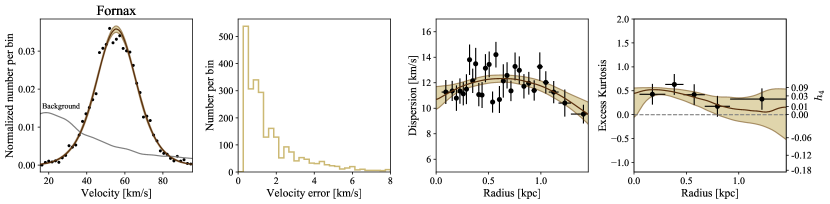
Figure 11: Similar to Fig. 7 but instead using a Gauss-Hermite series for positive excess kurtosis. Note in particular the different relationship between $\displaystyle h_{4}$ and the excess kurtosis for these models.

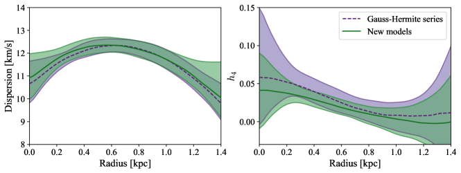
Figure 12: Comparison of the radial dispersion and $\displaystyle h_{4}$ profiles using the Gauss-Hermite series (dashed purple) and the Laplace kernel model (green solid) for positive $\displaystyle h_{4}$. The median and $\displaystyle\pm 1\sigma$ bands are shown.

When working with models with positive excess kurtosis, it is possible to use the Gauss-Hermite series as it is always positive definite for $\displaystyle h_{3}=0$ and $\displaystyle h_{4}>0$. In Fig. 11, we provide an alternative fit to the Fornax data using a Gauss-Hermite series instead of the Laplace kernel model introduced in this paper. Note that at equivalent $\displaystyle h_{4}$, the values of kurtosis admitted by the Gauss-Hermite series are smaller than for the Laplace kernel. However, as shown in Fig. 12, both models produce similar dispersion and $\displaystyle h_{4}$ profiles.

References

- Agnello et al. (2014) Agnello A., Evans N. W., Romanowsky A. J., Brodie J. P., 2014, MNRAS, 442, 3299
- Amorisco & Evans (2011) Amorisco N. C., Evans N. W., 2011, MNRAS, 411, 2118
- Amorisco & Evans (2012a) Amorisco N. C., Evans N. W., 2012a, MNRAS, 419, 184
- Amorisco & Evans (2012b) Amorisco N. C., Evans N. W., 2012b, MNRAS, 424, 1899
- Amorisco et al. (2013) Amorisco N. C., Agnello A., Evans N. W., 2013, MNRAS, 429, L89
- Astropy Collaboration et al. (2013) Astropy Collaboration et al., 2013, A&A, 558, A33
- Battaglia et al. (2006) Battaglia G., et al., 2006, A&A, 459, 423
- Bender et al. (1994) Bender R., Saglia R. P., Gerhard O. E., 1994, MNRAS, 269, 785
- Binney & Mamon (1982) Binney J., Mamon G. A., 1982, MNRAS, 200, 361
- Binney & Merrifield (1998) Binney J., Merrifield M., 1998, Galactic Astronomy. Princeton University Press
- Blinnikov & Moessner (1998) Blinnikov S., Moessner R., 1998, A&AS, 130, 193
- Breddels & Helmi (2013) Breddels M. A., Helmi A., 2013, A&A, 558, A35
- Cappellari (2017) Cappellari M., 2017, MNRAS, 466, 798
- Cappellari & Emsellem (2004) Cappellari M., Emsellem E., 2004, PASP, 116, 138
- Cappellari et al. (2011) Cappellari M., et al., 2011, MNRAS, 413, 813
- Debattista et al. (2005) Debattista V. P., Carollo C. M., Mayer L., Moore B., 2005, ApJ, 628, 678
- Emsellem et al. (2004) Emsellem E., et al., 2004, MNRAS, 352, 721
- Evans et al. (2009) Evans N. W., An J., Walker M. G., 2009, MNRAS, 393, L50
- Foreman-Mackey et al. (2013) Foreman-Mackey D., Hogg D. W., Lang D., Goodman J., 2013, PASP, 125, 306
- Gaia Collaboration et al. (2016) Gaia Collaboration et al., 2016, A&A, 595, A1
- Gaia Collaboration et al. (2018a) Gaia Collaboration et al., 2018a, A&A, 616, A1
- Gaia Collaboration et al. (2018b) Gaia Collaboration et al., 2018b, A&A, 616, A12
- Gerhard (1993) Gerhard O. E., 1993, MNRAS, 265, 213
- Gradshteyn & Ryzhik (2007) Gradshteyn I. S., Ryzhik I. M., 2007, Table of integrals, series, and products, 7th edn. Elsevier/Academic Press, Amsterdam
- Hunter (2007) Hunter J. D., 2007, Computing in Science Engineering, 9, 90
- Irwin & Hatzidimitriou (1995) Irwin M., Hatzidimitriou D., 1995, MNRAS, 277, 1354
- Kendall & Stuart (1977) Kendall M., Stuart A., 1977, The advanced theory of statistics. Vol.1: Distribution theory. Charles Griffin & Co.
- Kenney & Keeping (1951) Kenney J., Keeping E., 1951, Mathematics of Statistics. Pt. 2, 2nd ed., Princeton, NJ: Van Nostrand
- Kuijken & Merrifield (1993) Kuijken K., Merrifield M. R., 1993, MNRAS, 264, 712
- Łokas (2002) Łokas E. L., 2002, MNRAS, 333, 697
- Łokas (2009) Łokas E. L., 2009, MNRAS, 394, L102
- Łokas et al. (2005) Łokas E. L., Mamon G. A., Prada F., 2005, MNRAS, 363, 918
- Long & Murali (1992) Long K., Murali C., 1992, ApJ, 397, 44
- Massari et al. (2018) Massari D., Breddels M. A., Helmi A., Posti L., Brown A. G. A., Tolstoy E., 2018, Nature Astronomy, 2, 156
- Mateo (1998) Mateo M. L., 1998, ARA&A, 36, 435
- McConnachie (2012) McConnachie A. W., 2012, AJ, 144, 4
- McGough et al. (2020) McGough D. P., Evans N. W., Sanders J. L., 2020, MNRAS, 493, 2676
- Méndez-Abreu et al. (2019) Méndez-Abreu J., et al., 2019, MNRAS, 482, L118
- Merrifield & Kent (1990) Merrifield M. R., Kent S. M., 1990, AJ, 99, 1548
- Moskowitz & Walker (2020) Moskowitz A. G., Walker M. G., 2020, ApJ, 892, 27
- Navarro et al. (1997) Navarro J. F., Frenk C. S., White S. D. M., 1997, ApJ, 490, 493
- Oldham & Auger (2016) Oldham L. J., Auger M. W., 2016, MNRAS, 457, 421
- Olver et al. (2016) Olver F. W. J., Olde Daalhuis A. B., Lozier D. W., Schneider B. I., Boisvert R. F., Clark C. W., Miller B. R., Saunders B. V., 2016, NIST Digital Library of Mathematical Functions, http://dlmf.nist.gov/
- Pascale et al. (2018) Pascale R., Posti L., Nipoti C., Binney J., 2018, MNRAS, 480, 927
- Posti et al. (2015) Posti L., Binney J., Nipoti C., Ciotti L., 2015, MNRAS, 447, 3060
- Price-Whelan et al. (2018) Price-Whelan A. M., et al., 2018, AJ, 156, 123
- Read et al. (2019) Read J. I., Walker M. G., Steger P., 2019, MNRAS, 484, 1401
- Richardson & Fairbairn (2013) Richardson T., Fairbairn M., 2013, MNRAS, 432, 3361
- Rix et al. (1997) Rix H.-W., de Zeeuw P. T., Cretton N., van der Marel R. P., Carollo C. M., 1997, ApJ, 488, 702
- Rizzi et al. (2007) Rizzi L., Held E. V., Saviane I., Tully R. B., Gullieuszik M., 2007, MNRAS, 380, 1255
- Sellwood & Gerhard (2020) Sellwood J. A., Gerhard O., 2020, MNRAS, 495, 3175
- Sharma et al. (2011) Sharma S., Bland-Hawthorn J., Johnston K. V., Binney J., 2011, ApJ, 730, 3
- Vasiliev (2019) Vasiliev E., 2019, MNRAS, 482, 1525
- Vazdekis et al. (2010) Vazdekis A., Sánchez-Blázquez P., Falcón-Barroso J., Cenarro A. J., Beasley M. A., Cardiel N., Gorgas J., Peletier R. F., 2010, MNRAS, 404, 1639
- Virtanen et al. (2020) Virtanen P., et al., 2020, Nature Methods, 17, 261
- Walker & Peñarrubia (2011) Walker M. G., Peñarrubia J., 2011, ApJ, 742, 20
- Walker et al. (2008) Walker M. G., Mateo M., Olszewski E. W., 2008, ApJ, 688, L75
- Walker et al. (2009a) Walker M. G., Mateo M., Olszewski E. W., 2009a, AJ, 137, 3100
- Walker et al. (2009b) Walker M. G., Mateo M., Olszewski E. W., Sen B., Woodroofe M., 2009b, AJ, 137, 3109
- Wang et al. (2019) Wang M. Y., et al., 2019, ApJ, 881, 118
- Waskom et al. (2017) Waskom M., et al., 2017, seaborn: v0.8.1. Zenodo, doi:10.5281/zenodo.883859
- Williams & Evans (2015) Williams A. A., Evans N. W., 2015, MNRAS, 448, 1360
- Williams & Evans (2017) Williams A. A., Evans N. W., 2017, MNRAS, 469, 4414
- Wojtak & Łokas (2010) Wojtak R., Łokas E. L., 2010, MNRAS, 408, 2442
- Wolfram Research Inc. (2012) Wolfram Research Inc. 2012, Mathematica, Version 9. Champaign, IL
- van de Sande et al. (2017) van de Sande J., et al., 2017, ApJ, 835, 104
- van der Marel & Franx (1993) van der Marel R. P., Franx M., 1993, ApJ, 407, 525
- van der Marel et al. (1994) van der Marel R. P., Evans N. W., Rix H. W., White S. D. M., de Zeeuw T., 1994, MNRAS, 271, 99
- van der Marel et al. (1998) van der Marel R. P., Cretton N., de Zeeuw P. T., Rix H.-W., 1998, ApJ, 493, 613
- van der Walt et al. (2011) van der Walt S., Colbert S. C., Varoquaux G., 2011, Computing in Science Engineering, 13, 22