Dynamical fast flow generation/acceleration in dense degenerate two-fluid plasmas of astrophysical objects

Abstract

We have shown the generation/amplification of fast macro-scale plasma flows in the degenerate two-fluid astrophysical systems with initial turbulent (micro–scale) magnetic/velocity fields due to the Unified Reverse Dynamo/Dynamo mechanism. This process is simultaneous with and complementary to the micro-scale unified dynamo. It is found that the generation of macro–scale flows is an essential consequence of the magneto-fluid coupling; the generation of macro–scale fast flows and magnetic fields are simultaneous, they grow proportionately. The resulting dynamical flow acceleration is directly proportional to the initial turbulent magnetic (kinetic/magnetic) energy in degenerate e-i (degenerate e-p) astrophysical plasma; the process is very sensitive to both the degeneracy level of the system and the magneto-fluid coupling. In case of degenerate e-p plasma, for realistic physical parameters, there always exists such a real solution of dispersion relation for which the formation of strong macro-scale flow/outflow is guaranteed; the generated/accelerated locally super-Alfvénic flows are extremely fast with Alfvén Mach number $>10^{3}$ as observed in a variety of astrophysical outflows.

Keywords stars: evolution; stars: white dwarfs; stars: winds, outflows; galaxies: jets; plasmas

1 Introduction

Several recent studies were devoted to the mechanisms that explain flow/outflow formations in stellar atmospheres. Flows as well as transient jets are observed in solar atmosphere – their role in the dynamics and heating of multi-scale complex-structure solar corona is already well appreciated. Flows are found crucial in astrophysical disks [see e.g. (Krishan & Yoshida, 2006; Zanni et al, 2007), (Shatashvili & Yoshida, 2011),
(Bodo et al, 2015) and references therein] and their corona, in inter- and extra-galactic environments. More extended large scale outflows are met in various astrophysical settings, e.g. AGN relativistic jets, protostellar jets, being the collimated long-lived structures related to accreting disks surrounding the compact objects [see e.g. (Begelman et al, 1984) and references therein]. In this view, in addition to the study of star evolution dynamics, it is important to uncover the contribution (if any) of flow dynamics in compact objects outer layers to the formation of large-scale jets/outflows.

Study of the multi-scale dynamics of compact object’s multi-component magnetospheres attracted the interest to solve phenomena related to star evolution problem. Among these investigations the studies on equilibrium structure formations based on so called Beltrami-Bernoulli (BB) class of equilibria model (Shiraishi et al, 2009; Iqbal et al, 2008; Pino et al, 2010; Mahajan & Lingam, 2015) opened the new channels for exploring the heating of atmospheres as well as the problems of large-scale magnetic and/or velocity field generation (Mahajan et al, 2001; Yoshida et al, 2001); Ohsaki et al 2001, (2002); (Mahajan et al, 2002),
(Mahajan et al 2005;, 2006); protostellar disk-jet structure formation (Arshilava et al., 2019). The examination of BB states were also performed for highly dense and degenerate plasmas applicable to compact star conditions (mean inter-particle distance is smaller than the de Broglie thermal wavelength so that particle energy distribution was dictated by Fermi-Dirac statistics) [see (Berezhiani et al 2015b, ) and references therein]. Such highly dense/degenerate plasmas are also found in various astrophysical / cosmological environments, in laboratories devoted to inertial confinement, in high energy density physics (Dunne, 2006; Mourou et al, 2006; Yanovsky et al, 2008; Tajima, 2014).

The density (determinant of degeneracy level) varies over many orders of magnitude in astro-settings. Compact astrophysical objects like white and brown dwarfs, neutron stars, magnetars with characteristic electron number densities within $(10^{26}--10^{32})\,cm^{-3}$ are the natural habitats for degenerate matter
(Chandrasekhar, 1931, 1939);
(Shapiro & Teukolsky, 1973; Begelman et al, 1984);
(Michel, 1982; Koester & Chanmugam, 1990);
(Michel, 1991; Beloborodov & Thompson, 2007);
(Shukla & Eliasson, 2010, 2011).
Rest frame e-p density near pulsar surface $\geq 10^{11}\,cm^{-3}$ (Gedalin et al, 1998), while in the MeV epoch of the early Universe, it can be $10^{32}\,cm^{-3}$ (Weinberg, 1972). Intense e-p pair creation takes place during the gravitational collapse of massive stars (Tsintsadze et al., 2003) with estimated density $\sim 10^{34}\,cm^{-3}$  (Han et al, 2012). In GRB sources (Aksenov et al, 2010) there may exist a superdense e-p plasma with density $(10^{30}-10^{37})\,cm^{-3}$. The consequences of degeneracy in a multi-component plasma was extensively studied recently in terms of multi-scale behavior accessible to such systems (Berezhiani et al 2015a, ; Shatashvili et al, 2016),
(Barnaveli & Shatashvili, 2017) to explore its role in the dynamics of star collapse while contraction of its atmosphere; to predict various phenomena in pre-compact era, or the compact objects’ dynamics since cooling process seems to be sensitive to outer layers/atmosphere composition, structure and their conditions.

Up to now there doesn’t exist a precise model of atmospheres of White Dwarfs (WDs) although recent studies show that a significant fraction of White Dwarfs are found to be magnetic. Massive and cool White Dwarfs are found with high ($>1\,KG$) fields detected [see (Winget & Kepler, 2008; Kepler et al, 2013, and references therein)]. Interestingly, the electron degeneracy manifests, explicitly, only through the Bernoulli condition for the case of mildly degenerate e-i plasma (Berezhiani et al 2015a, ), and as a result, such gas can sustain a qualitatively new state: a nontrivial Double BB equilibrium at zero temperature. It is extremely interesting how this effect will manifest or define the fate of Unified Dynamo/RD process (Mahajan et al 2005;, 2006; Lingam & Mahajan, 2015), specifically in view of flow generation in the vicinity of compact object, in several other astrophysical setups.

In (Barnaveli & Shatashvili, 2017) the fast flow generation due to magneto-fluid coupling (through catastrophe) near the surface of dense degenerate e-i stellar atmospheres was suggested finding that distance over which acceleration appears is determined by the strength of gravity and degeneracy parameter. Application of this mechanism for White Dwarfs’ atmospheres was examined showing the possibility of the super-Alfvénic flow generation for various surface parameters of WDs; the simultaneous possibility of flow acceleration and magnetic field amplification for specific boundary conditions was explored in which the degeneracy has a striking effect. For the understanding of origin and evolution of dense compact objects; for their cooling and accretion dynamics; to know the magnetic fields dynamics/fate the inclusion of time-dependency may become determining and crucial – the unified Dynamo / Reverse Dynamo treatment (Mahajan et al 2005;, 2006; Lingam & Mahajan, 2015) can lead to additional significant effects on the formation of large-scale flows and/or magnetic fields in astrophysical objects with degenerate plasmas (e.g. outer layers of compact objects).

The goal of present study is to explore the role of degeneracy in the dynamical fast flow formation for degenerate plasmas of astrophysical objects; we will follow the methodology of Reverse Dynamo (RD) mechanism proposed in (Mahajan et al. 2005) (demonstrating that dynamo and RD operate simultaneously). RD – permanent dynamical feeding of flow kinetic energy through an interaction of microscopic magnetic field structures with weak flows was shown to be universal property (indicating application for Solar atmosphere). (Lingam & Mahajan, 2015) conjectured that an efficient RD may be the source of observed astrophysical outflows with Alfvén Mach number $\gg 1$. Due to the existence of an intrinsic micro–scale in HMHD at which ion / degenerate e-p kinetic inertia effects become important it is possible to characterize long and short scales in a well defined way (the macroscopic scale of the system is generally much larger than the charged fluid skin depth). We will examine the possible role played by Unified Dynamo/RD mechanism in explaining the existence of large-scale velocity and magnetic fields in degenerate two-fluid plasmas of astrophysical objects. We will find the applications for: 1) WDs with degenerate electrons and classical ions assuming the density variations to be slow below the catastrophe heights (Barnaveli & Shatashvili, 2017); 2) astrophysical objects with degenerate e-p plasma for which the degeneracy effects become crucial when the inertia of bulk e-p components makes the effective skin depths much larger than the standard skin depth (Shatashvili et al, 2016).

2 Model Equations for Unified Reverse Dynamo / Dynamo mechanism for WDs

In this section we start from the outer layers of compact objects, specifically the case of WDs’ – end product of the star accretion evolution – that are considered to be stellar remnants featuring global magnetic structures with field strengths within $1\,kG\div 1000\,MG$ (Liebert et al, 2003; Kawka et al, 2007). Most of these objects are higher-field magnetic WDs; a distribution of magnetic field strengths appears to peak around $B>20\,MG$ (Schmidt et al, 2003; Külebi et al, 2009). In (Kawka & Vennes, 2014) it was shown that WD stars with developed convective zones show stronger magnetic fields than hotter stars; the mean mass of magnetic stars is on average larger than the mean mass of nonmagnetic WD stars. The effective temperatures of convective hydrogen-line (DA) white dwarfs are in the range $(6000-15000)\,K$ and convective velocities are of the order of $\sim 1\,km/s$ at the base of the convection zone reaching maximum value $6\,km/s$ (Tremblay et al, 2015, and references therein); while for cool, magnetic, polluted hydrogen atmosphere WDs (DAs) it was found to be $(19.8\pm 1.7)\,km/s$ (Kawka & Vennes, 2014, and references therein). Many WDs have much stronger ($\gtrsim 3$ MG) surface magnetic fields; this could be partially explained by the core dynamo-generated fields (Ferrario et al, 2015). Even stronger ($\gtrsim 10^{6}$ G) magnetic fields could be confined within the WD’s interior and not detectable at the surface even as they cool (Cumming, 2002). Then, it is expected that the dynamical evolution of WD’s convective envelope / outer layers may define the final structure of its interior as well as of atmosphere (Barnaveli & Shatashvili, 2017).

The simplified HMHD of (Berezhiani et al 2015a, ) for a two-species system of non-degenerate non relativistic ions, and degenerate relativistic electrons embedded in a magnetic field – a minimal model that contains two disparate interacting scales – can be useful for studying the Unified RD/Dynamo in WD’s outer layers. In this model the ion ($v$) and degenerate electron (${\mbox{\boldmath$v$}}_{e}={\mbox{\boldmath$v$}}-{\bf j}/eN$) flow velocities are different even in the limit of zero electron inertia. In its dimensionless form, HMHD equations for degenerate electron-ion plasma reduce to:

$$\frac{\partial\boldsymbol{b}}{\partial t}=\nabla\times\left[\left(\boldsymbol{v}-\frac{\alpha}{N}\left(\nabla\times\boldsymbol{b}\right)\right)\times\boldsymbol{b}\right]\ ,$$ (1)

$\displaystyle\hskip 0.0pt{\frac{\partial\boldsymbol{v}}{\partial t}=\frac{1}{N}\left(\nabla\boldsymbol{\times}\boldsymbol{b}\right)\boldsymbol{\times}\boldsymbol{b}+\boldsymbol{v}\boldsymbol{\times}\nabla\boldsymbol{\times}\boldsymbol{v}}$

$$\qquad-\nabla\left({\beta}_{0}{lnN\ }-{\mu}_{0}\left(G_{d}\gamma\right)+\frac{{\boldsymbol{v}}^{\boldsymbol{2}}}{2}-\frac{R_{A}}{R}\right)\ .$$ (2)

where  ${\boldsymbol{b}}=e{\bf B}/m_{i}c$  and it was assumed, that electron and proton laboratory-frame densities are nearly equal - $N_{e}\simeq N_{i}=N$  [rest-frame density  $n=N/\gamma({\mbox{\boldmath$v$}})$  with  $\gamma({\mbox{\boldmath$v$}})\simeq\gamma_{e}$  being a Lorentz factor for electrons]; the density is normalized to $N_{0}$ (the corresponding rest-frame density is  $n_{0}$); the magnetic field is normalized to some ambient $B_{0}$ ; all velocities are measured in terms of the corresponding Alfvén speed  $V_{A}=B_{0}/\sqrt{4\pi N_{0}m_{i}}$ ; all lengths are normalized to the characteristic length-scale of the system, WD-radius $R_{w}$. $\beta_{0}$ is an equilibrium plasma beta;  $\mu_{0}=m_{e}c^{2}/m_{i}V_{A}^{2}$ ;  $R$ is the radial distance from the center of WD normalized to its radius  $R_{W}\ [\sim(0.008-0.02)\ R_{\odot}]$ and $R_{A}=GM_{W}/R_{W}V_{A}^{2}$ ($G$ – gravitational constant, $M_{W}$ – WD mass); dimensionless parameter $\alpha=\lambda_{i}/R_{w}$ . Here the ion-skin-depth $\lambda_{i}=c/\omega_{pi}\sim(10^{-5}-10^{-7})\,cm$ for a typical cold magnetic WDs with degenerate electron densities $\sim(10^{25}-10^{29})\,cm^{-3}$ and magnetic fields $\sim(10^{5}-10^{9})\,G$, temperatures  $\sim(40000-6000)\,K$. The degeneracy induced effective mass factor for strongly degenerate electron plasma is determined by the plasma rest frame density, $G_{d}=[1+(n/n_{c})^{2/3}]^{1/2}$  for arbitrary  $n/n_{c}$,  with  $n_{c}=5.9\times 10^{29}cm^{-3}$ being the critical number-density. Comparing the terms in total pressure on the r.h.s. of (2) for above parameters, one can see the dominance of electron fluid degeneracy pressure.

Following the standard procedure (Mahajan et al. 2005)) let’s assume that our total fields are composed of some ambient seed fields as well as density and fluctuations about them with account of degeneracy effects:

$$n=n_{0}+\delta n\ ;\quad\boldsymbol{b}={\boldsymbol{b}}_{\boldsymbol{0}}+\boldsymbol{H}+\tilde{\boldsymbol{b}}\ ,\quad\boldsymbol{v}={\boldsymbol{v}}_{\boldsymbol{0}}+\boldsymbol{U}+\tilde{\boldsymbol{v}}\ ,$$ (3)

where $n_{0}=const,\ {\boldsymbol{b}}_{\boldsymbol{0}}$ ,  ${\boldsymbol{v}}_{\boldsymbol{0}}$ are equilibrium density and the equilibrium fields; $\boldsymbol{H}$ , $\boldsymbol{U}$ , $\delta n$ are the macroscopic fluctuations; and $\tilde{\boldsymbol{b}}$, $\tilde{\boldsymbol{v}}$ are the microscopic fluctuations, respectively; we have ignored the microscopic density fluctuation due to its higher order contribution; also the wave coupling is beyond the scope of this study. We emphasize here, that the energy reservoir comes from the background fields that may have both macro-scale and micro-scale components. Their energy feeds the macro- and micro-scale fluctuations of density and fields. It is natural to assume that in HMHD the equilibrium fields are the solutions of so called Double Beltrami Equations (Mahajan & Yoshida, 1998; Mahajan et al, 2001; Mahajan et al 2005;, 2006):

$$\boldsymbol{b}_{0}=a\left(\boldsymbol{v}_{0}-\alpha\,\nabla\times\boldsymbol{b}_{0}\right)\ ,\ \ \ \boldsymbol{b}_{0}+\alpha\,\nabla\times\boldsymbol{v}_{0}=d\boldsymbol{v}_{0}\boldsymbol{\ },$$ (4)

together with the Bernoulli Condition (at  ${\beta}_{0}{ln{N}\ }\ll{\mu}_{0}\,G_{d}(N)\gamma\ ,\ \gamma({\mbox{\boldmath$v$}})\sim 1$  for our problem of interest):

$$\nabla\left({\mu}_{0}G_{d}(\delta n)+\frac{{{\boldsymbol{v}}_{\boldsymbol{0}}}^{\boldsymbol{2}}}{2}-\frac{R_{A}}{R}\right)=0\ ,$$ (5)

where  $a$  and  $d$  are dimensionless constants related to the two invariants: the magnetic helicity  $h_{1}=\int{({\bf A}\cdot{\bf b})\,d^{3}x}$  and the generalized helicity  $h_{2}=\int{({\bf A}+{\boldsymbol{v}})\cdot({\bf b}+\nabla\times\boldsymbol{v})\,d^{3}x}$  of the system with  ${\bf A}$  being the dimensionless vector potential. Notice, that in this approximation the electron vorticity is primarily magnetic  (${\boldsymbol{b}}_{0}$)  while the ion vorticity  (${\mbox{\boldmath$b$}}_{0}+\nabla\times{\mbox{\boldmath$v$}}_{0}$) has both kinematic and magnetic parts. In (Barnaveli & Shatashvili, 2017) it was shown that due to the degenerate density both the velocity and magnetic fields undergo catastrophe at some height from the WD’s surface. In present paper we assume that the distances are below this point so that macro-scale fluctuations of density and fields are slowly varying functions. Also, for simplicity we assume that our zeroth-order fields are wholly at the microscopic scale. This allows us to create a hierarchy in the micro–fields; the ambient fields are much greater than the fluctuations at the same scale  ($|\tilde{\mbox{\boldmath$b$}}|\ll|{\mbox{\boldmath$b$}}_{0}|,|\tilde{\mbox{\boldmath$v$}}|\ll|{\mbox{\boldmath$v$}}_{0}|$). This closure model accounts properly the self-consistent feedback of the micro–scale in the evolution of both macro-scale fields ${\bf H}$ and ${\bf U}$, as well as the role of the Hall current (especially in the dynamics of the micro–scale) [see Mininni et al. 2003, Mahajan et al. 2005 for details].

The invariant helicities control the final results through the Beltrami scales $a$ and $d$. We choose these constants so that the characteristic scales [inverse of  ${\frac{1}{2}}[(d-a^{-1})\pm((d+a^{-1})^{2}-4)^{-1/2}]$ ] become vastly separated (Mahajan & Yoshida, 1998; Mahajan et al, 2001). In the astrophysically relevant regime of disparate scales (the size of the structure is much greater than the ion skin depth), we deal with two extreme cases (in the analysis below we use $\lambda$ for the micro-scale and $\mu$ for the macro-scale): (1) $a\sim d\gg 1$ and ($(a-d)/ad\ll 1$ [$\lambda\sim d$ and $\mu\sim(a-d)/ad$ ], and (2) $a\sim d\ll 1$ and ($a-d)/ad\gg 1$ [$\lambda\sim a-a^{-1}$ and $\mu\sim d-a$].

Astrophysical objects, including compact stars like WD are macro-scale, then, consistent with the main objectives of this paper, we assume that basic reservoir [from which system generates macro-scale fields] is at micro-scale; neglecting macro-scale equilibrium component we find that the velocity and magnetic fields get linearly related as  ${\boldsymbol{v}}_{0}=(\lambda+a^{-1}){\boldsymbol{b}}_{0}$  yielding  ${\boldsymbol{v}}_{0e}={\boldsymbol{v}}_{0}-\alpha\nabla\times{\boldsymbol{b}}_{0}={(\lambda+a^{-1})\boldsymbol{b}}_{0}-\lambda{\boldsymbol{b}}_{0}={a^{-1}\boldsymbol{b}}_{0}$  and leading to

$$\dot{\tilde{\boldsymbol{b}}}=({a^{-1}}{\boldsymbol{H}}-{\boldsymbol{U}})\cdot\nabla{\boldsymbol{b}}_{0}\ ,$$ (6)

$$\dot{\tilde{\boldsymbol{v}}}=({\boldsymbol{H}}-(\lambda+a^{-1}){\boldsymbol{U})\cdot\nabla{\boldsymbol{b}}_{0}}\ .$$ (7)

Using (6,7) we obtain for macro-scale fields following:

$$\ddot{\boldsymbol{H}}=r\,\nabla\times\boldsymbol{H}\ ,\qquad\ddot{\boldsymbol{U}}=-\ \nabla\times(s\,\boldsymbol{U}-q\,\boldsymbol{H})\ ,$$ (8)

where the constants $q$, $r$ and $s$ :

$\displaystyle\hskip 0.0pt{q=\lambda^{2}\frac{b_{0}^{2}}{6}\ ,\qquad r=-\lambda\frac{b_{0}^{2}}{3}(1-\lambda{a^{-1}}-{a^{-2}})\ ,}$

$$s=\lambda\frac{b_{0}^{2}}{6}\left[{({\lambda+a^{-1}}})^{2}-1\right]$$ (9)

are determined by DB parameters $a$ and $d$ (hence, by the ambient magnetic and generalized helicities) and scales directly with the ambient turbulent energy $\sim{\boldsymbol{b}}_{0}^{2}$ (${\boldsymbol{v}_{0}^{2}}$). Performing Fourier analysis, we obtain:

$$\boldsymbol{U}=\frac{q}{s+r}\boldsymbol{H}\ .$$ (10)

From Equations (8, 9, 10) we observe that, to leading order, like in classical case (Mahajan et al 2005;, 2006), ${\boldsymbol{H}}$ evolves independently of ${\boldsymbol{U}}$, but the reverse is not true: the evolution of ${\boldsymbol{U}}$ does require knowledge of ${\boldsymbol{H}}$. Hence, a choice of Beltrami scales $a$ and $d$ that now reflect the helicities of degenerate e-i system, fixes the relative amounts in ambient fields’ microscopic energy and, consequently, in the generated macroscopic fields that grow proportionately to each other. In the subsection below we show that the Unified RD/D mechanism affects the evolution picture of outer layers of magnetic White Dwarfs (WD) predicted in (Berezhiani et al 2015a, ; Shatashvili et al, 2016) where it was shown that when the star contracts its outer layer keeps the multi-structure character although density in structures becomes defined by electron degeneracy pressure.

2.1 Reverse Dynamo for WDs’ degenerate electron-ion plasma

We can examine the two observationally justified extreme cases for Beltrami scales:

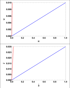
Fig. 1 : Evolution of generated velocity and magnetic fluctuations (blue lines) for Beltrami Parameneters $a\sim d=100$: top panel shows the macro-scale velocity field ${\boldsymbol{U}}$ versus macro-scale magnetic field ${\boldsymbol{H}}$ while the bottom panel shows the micro-scale ${\boldsymbol{\tilde{v}}}$ versus micro-scale ${\boldsymbol{\tilde{b}}}$. Starting from strongly super-Alfvénic ambient flow system arrives to sub-A;fvénic macro-scale and micro-scale fluctuations, locally. Straight Dynamo for both scales. Dotted lines in red show the Alffvénic flow for both scales, respectively.

Fig. 2 : Plot for Alfvén Mach Number versus $a>1$ for macro-scale vector-fields $M_{A}$ (top) and micro-scale vector-fields ${\tilde{M}}_{A}$ (bottom), respectively for generated velocity and magnetic fluctuations. Bigger the Beltrami scale $a$ smaller is the Alfvén Mach number that is $\ll 1$ for all $a$-s. For both scales the Straight Dynamo scenario works showing that Strong Magnetic fields (both macro– and micro– scales) are generated from primarily kinetic micro-scale ambient state.

(1) Example of primarily kinetic ambient fields: $a\sim d\gg 1\ ,\ (\lambda\sim a\gg 1)$ implying ${\boldsymbol{v}}_{0}=(\lambda+a^{-1}){\boldsymbol{b}}_{0}\sim a\,\boldsymbol{b}_{0}\gg\boldsymbol{b}_{0}$. Such conditions may be met in WD’s photospheres, where the turbulent velocity field at some stage can be dominant, although some $\boldsymbol{b}_{0}$ is present as well. For these parameters, the generated macro-fields have precisely the opposite ordering, $\boldsymbol{U}\sim a^{-1}\boldsymbol{H}\ll\boldsymbol{H}$. In this junction it is interesting to recall that recent studies show that a significant fraction of WDs are found to have rather strong surface magnetic fields (see (Kepler et al, 2013; Hollands et al, 2015; Barnaveli & Shatashvili, 2017) and references therein). One of the evolution channels could be the amplification of a seed field by a convective dynamo in the core -envelope boundary of the evolved progenitors (Ruderman & Sutherland 1973; Kissin & Thompson 2015). It is, therefore, very important to show that the effects of magneto-fluid couplings in outer layers of accreting stars may lead to the dynamical evolution of their convective envelopes and generate macro-scale magnetic field through macro-scale Dynamo mechanism. Our analysis show that this process is maintained through the generation of micro-scale fluctuations ${\boldsymbol{\tilde{v}}}$ and ${\boldsymbol{\tilde{b}}}$. In Fig.1 the relevant plots are presented. Fig.2 gives the results for so called Alfvén Mach Number versus Beltrami scale $a>1$ for macro-scale vector-fields ($M_{A}$) and micro-scale vector-fields (${\tilde{M}}_{A}$), respectively. We see, that starting from primarily super-Alfvénic micro-scale flows the magneto-fluid coupling guarantees the straight Dynamo scenario – the generated fields are sub-Alfvénic in both scales. Created macro(micro)–scale flows and Magnetic fields are defined by ambient densities and velocity/magnetic fields (ambient Alfvén Velocity) as well as Beltrami parameters (helicities) – such situation may be met in the poles of magnetic WD’s or for WDs with not detectable surface magnetic fields.

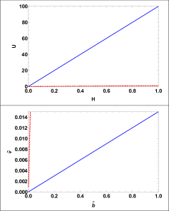
Fig. 3 : Evolution of generated velocity and magnetic fluctuations (blue lines) for Beltrami Parameneters $a\sim d=0.01$: top panel shows the macro-scale velocity field ${\boldsymbol{U}}$ versus macro-scale magnetic field ${\boldsymbol{H}}$ while the bottom panel shows the micro-scale ${\boldsymbol{\tilde{v}}}$ versus micro-scale ${\boldsymbol{\tilde{b}}}$. Starting from sub-Alfvénic ambient micro-flow system arrives to strongly super-A;fvénic macro-scale and sub-Alfvénic micro-scale fluctuation, locally. Reverse Dynamo for macro–scale and Straight Dynamo for micro-scale. Dotted lines in red show the Alffvénic flow for both scales, respectively.

Fig. 4 : Plot for Alfvén Mach Number versus $a<1$ for macro-scale vector-fields $M_{A}$ (top) and micro-scale vector-fields ${\tilde{M}}_{A}$ (bottom), respectively for generated velocity and magnetic fluctuations. Smaller the Beltrami scale $a$ bigger is the Macro-scale Alfvén Mach number that is $\gg 1$ for all $a$-s in range while for micro-scale situation reverses – Manifestation of Unified Reverse Dynamo/Dynamo mechanism.

(2) Example of primarily magnetic ambient fields: $a\sim d\ \ll 1,(\lambda=a-a^{-1}\gg 1)$ implying ${\boldsymbol{v}}_{0}=(\lambda+a^{-1}){\boldsymbol{b}}_{0}\sim a\,\boldsymbol{b}_{0}\ll\boldsymbol{b}_{0}$. These conditions maybe met in WD’s photospheres’ certain convective areas where a strongly sub-Alfveńic turbulent flow may exist. This micro-scale magnetically dominant initial system creates macroscale fields $\boldsymbol{U}\sim a^{-1}\boldsymbol{H}\gg\boldsymbol{H}$ that are kinetically abundant – Reverse Dynamo scenario: in the given region of WD’s photosphere where the fluctuating/turbulent magnetic field is initially dominant, the magneto-fluid coupling induces efficient/significant acceleration, and part of the magnetic energy will be transferred to steady plasma flows that are strongly super-Alfveńic; process is accompanied by a weak macro-scale magnetic field generation. In this regime generated micro-fields remain magnetically dominated, hence defining the Unified Reverse Dynamo/Dynamo mechanism in its full strength (see Fig.3 and Fig.4). It is interesting that this mechanism works for any level of degeneracy and may help us to predict the jet/outflow origin in the atmospheres/outer layers of WD’s.

3 Model Equations for RD for Degenerate e-p Astrophysical Plasmas

The dynamical phenomena in e-p plasmas develop differently from their counterparts in the usual e-i system. The annihilation, which takes place in the interaction of electrons and positrons occurs at much longer characteristic time scales compared with the time in which the collective interaction between the charged particles takes place; the details of such processes in super-dense e-p plasma can be found in (Berezhiani et al. 2015b, and references therein). Notice that even with equal effective masses at equal temperatures, inertia change due to degeneracy can cause asymmetry in e-p fluid (Mahajan & Lingam, 2015); the degenerate e-p system is capable of creating length scales larger than its classical counterpart through the degeneracy enhanced inertia of the particles (Shatashvili et al, 2016); this scale turns out to be degeneracy dependent. Using this formalism, introducing the e-p plasma bulk velocity as ${\bf V}=\frac{1}{2}({\bf V}_{+}+{\bf V}_{-})$, assuming $\gamma_{-}\sim\gamma_{+}\sim 1;\ N_{-}=N_{+}\equiv N$ leading to $G_{-}\equiv G_{+}\equiv G_{0}(n)=const$ we derive the equations to describe the dynamics of such system:

$\displaystyle\hskip 0.0pt{\frac{\partial{\bf V}}{\partial t}={\bf V}\times\nabla\times{\bf V}\ +\ (\nabla\times{\bf b})\times{\bf b}}$

$$\qquad\qquad+\ \alpha^{2}(\nabla\times{\bf b})\times\nabla\times\nabla\times{\bf b}\ ,$$ (11)

$\displaystyle\hskip 0.0pt{\frac{\partial{\bf b}}{\partial t}\ +\ \alpha^{2}\frac{\partial}{\partial t}\nabla\times\nabla\times{\bf b}=\nabla\times({\bf V}\times{\bf b})}$

$$+\ \alpha^{2}\nabla\times({\bf V}\times\nabla\times\nabla\times{\bf b}\ +\ \nabla\times{\bf b}\times\nabla\times{\bf V})\ ,$$ (12)

where all velocities are measured in terms of the corresponding Alfvén velocity  $V_{A}=\frac{B_{0}}{\sqrt{8\pi n_{0}mG_{0}}}$ , all lengths are normalized to some characteristic length $L$ (e.g. radius of the compact star); $\alpha=\lambda_{\rm{eff}}/L$ with $\lambda_{\rm{eff}}$ being an ”effective” electron (positron) skin depth – $\lambda_{\rm{eff}}=\frac{1}{\sqrt{2}}\frac{c}{\omega_{p}}=c\sqrt{\frac{mG_{0}}{8\pi n_{0}e^{2}}}$. In such degenerate e-p plasma the equilibrium state constiututes the Triple-Beltrami structures with 3 different scales. Then, following the standard procedure, introducing for velocity and magnetic fields similar to (3) representations, we use equilibrium equations from (Shatashvili et al, 2016):

$\displaystyle\hskip 0.0pt{2G_{0}^{2}\nabla\times\nabla\times\nabla\times{\bf b}_{0}-2G_{0}(a_{+}-a_{-})\,\nabla\times\nabla\times{\bf b}_{0}}$

$$+2G_{0}(G_{0}-a_{+}a_{-})\,\nabla\times{\bf b}_{0}-(a_{+}-a_{-})\,{\bf b}_{0}=0\ ,$$ (13)

$${\bf V}_{0}=(a_{+}+a_{-})^{-1}(2G_{0}\nabla\times\nabla\times{\bf b}_{0})$$ (14)

$\displaystyle\hskip 0.0pt{\qquad-(a_{+}+a_{-})^{-1}\left[(a_{+}-a_{-})\nabla\times{\bf b}_{0}+2{\bf b}_{0}\right]\ ,}$

where $a_{\pm}$ are dimensionless constants related to two invariants:  $h_{\pm}=\int{({\bf A}\pm G_{0}{\bf V}_{\pm})\cdot({\bf b}\pm G_{0}\nabla\times{\bf V}_{\pm})\,d^{3}x}$ – the generalized helicities of the system. Here the generalized vorticities for both fluids have now both magnetic and kinetic parts due to the degeneracy effects. We need to choose these constants so that the scales [solutions of the equation  $2G_{0}^{2}\,\mu^{3}-2G_{0}(a_{+}-a_{-})\,\mu^{2}+2G_{0}(G_{0}-a_{+}a_{-})\,\mu-(a_{+}-a_{-})=0$]  are vastly separated. For the analysis we choose the simplest case when $a_{+}\sim a_{-}\simeq a$, then the three real roots are:  $0;\ \pm\sqrt{a^{2}-G_{0}}/G_{0}$  with the condition $a^{2}>G_{0}$. Following the similar to Section 2 procedure we assume that the basic reservoir is fully micro-scale leading to the velocity and magnetic fields being linearly related as ${\bf V}_{0}=\frac{a}{G_{0}}{\bf b}_{0}$ when choosing the inverse micro-scale to be $\lambda=\sqrt{a^{2}-G_{0}}/G_{0}$. Note, that when $a>G_{0}$ the ambient micro-scale fields are primarily kinetic, while at $\sqrt{G_{0}}<a<G_{0}$ they are primarily magnetic.

The straightforward algebra leads to the following equations for micro-scale and macro-scale fluctuations [${\bf Q}$ and ${\bf S}$ are the functions containing $U$ and $H$]:

$$\frac{\partial{\tilde{\bf b}}}{\partial t}=({\bf Q}\cdot\nabla){\bf b}_{0}\ ,\qquad\frac{\partial{\tilde{\bf V}}}{\partial t}=({\bf S}\cdot\nabla)\,{\bf b}_{0}\ ,$$ (15)

and

$$\ddot{\bf H}=r\nabla\times{\bf H}+m\nabla\times\nabla\times{\bf H}+\nu\nabla\times\nabla\times{\bf U}\ ,$$ (16)

$$\ddot{\bf U}=s\nabla\times{\bf U}+q\nabla\times{\bf H}+l\nabla\times\nabla\times{\bf U}+p\nabla\times\nabla\times{\bf H}$$ (17)

where:

$\displaystyle\hskip 0.0pt{r\equiv\frac{\lambda b_{0}^{2}}{3}\left[\left(\frac{a}{G_{0}}\right)^{2}-1-\lambda^{2}\right],\quad l\equiv-\alpha\,\frac{\lambda^{2}b_{0}^{2}}{6}(2+3\lambda^{2}),}$

$\displaystyle\hskip 0.0pt{\nu\equiv\alpha\,\frac{\lambda^{2}b_{0}^{2}}{6}\left(\frac{a}{G_{0}}\right)\,(3+2\lambda^{2}),\ \ q\equiv-\left(\frac{a}{G_{0}}\right)\frac{\lambda^{3}b_{0}^{2}}{3},}$

$\displaystyle\hskip 0.0pt{p\equiv\alpha\,\frac{\lambda^{2}b_{0}^{2}}{3}\left(\frac{a}{G_{0}}\right)(1+\lambda^{2}),\ \ \nu=p+\alpha\,\frac{\lambda^{2}b_{0}^{2}}{6}\left(\frac{a}{G_{0}}\right),}$

$\displaystyle\hskip 0.0pt{s\equiv\frac{\lambda b_{0}^{2}}{6}\left[1-\left(\frac{a}{G_{0}}\right)^{2}+3\lambda^{3}+2\lambda^{4}\right],}$

$$m\equiv\alpha\frac{\lambda^{2}b_{0}^{2}}{6}\left[1-4\left(\frac{a}{G_{0}}\right)^{2}\right]\ .$$ (18)

Performing a Fourier analysis we obtain the following dispersion relation:

$$\qquad\qquad D^{2}(\omega,k)=C^{2}(\omega,k)\,k^{2},\quad{\rm with}$$ (19)

$\displaystyle\hskip 0.0pt{D(\omega,k)=\Big{(}(\omega^{2}+lk^{2})(\omega^{2}+mk^{2})+rsk^{2}-p\nu k^{4}\Big{)},}$

$\displaystyle\hskip 0.0pt{C(\omega,k)=\Big{(}(\omega^{2}+lk^{2})r+(\omega^{2}+mk^{2})s-q\nu k^{2}\Big{)},}$

and, finally, the relation for macro-scale fluctuations:

$$\qquad\qquad{\bf U}=\frac{[r\,C-(mk^{2}-\omega^{2})\,D]}{\nu k^{2}\,D}\,{\bf H}\ .$$ (20)

We observe that to leading order, unlike the degenerate e-i case, the evolution of ${\bf H}$ does require knowledge of ${\bf U}$ and vice versa; a choice of Beltrami parameter $a$ (that now reflects the helicities of degenerate e-p system) as well as the density (through effective mass $G_{0}$), fixes the relative amounts in ambient fields’ microscopic energy and, consequently, in the generated macroscopic fields that grow proportionately to each other. Below we show how the Unified RD/Dynamo mechanism affects the evolution picture of astrophysical objects with degenerate e–p plasmas.

3.1 Unified Dynamo/Reverse Dynamo mechanism for Degenerate e-p astrophysical plasmas

As discussed above, super-dense e -p astrophysical plasma density is argued to be in the range $n=(10^{30}-10^{37})\,cm^{-3}$. E.g. the effective mass $G_{0}\sim 25$ for the density $\sim 10^{34}\,cm^{-3}$. Then, for such objects we can examine the two extreme cases for Beltrami parameter: (1) $a\sim 100\gg G_{0}$ and (2) $\sqrt{G_{0}}<a\sim 10<G_{0}$. Since $\alpha$ - Hall term contribution - is very small (in the simulations we are using $\alpha\sim 10^{-6}$ ) the coefficients $l,\ p,\ q,\ m,\nu$ are normally small; coefficients $r$ and $s$ are free of $\alpha$, so they may become the determining ones in the dispersion as well as in the ratio for generated fluctuations. Also, since inverse micro-scale $\lambda=\frac{a}{G}\sqrt{1-\frac{G_{0}}{a^{2}}}$, we have $r<0$ in our analysis (defining the growth rate of generated macro-fields via dispersion relation).

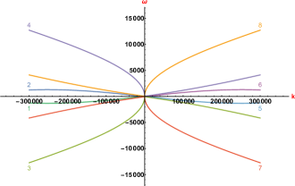
Fig. 5 : Solution of dispersion relation (19) for $a=100,G_{0}=25$ ; 8 different real roots are displayed by different color.

Fig. 6 : Plot for Alfvén Mach Numbers versus $k$ for: macro-scale vector-fields $M_{A}$ (top) and micro-scale vector-fields ${\tilde{M}_{A}}$ (bottom), respectively for generated velocity and magnetic fluctuations for the root 6 of Fig.5; $a=100>G_{0}=25$. Bigger the $k$ smaller is $M_{A}$ but still $\ll 1$ ; both scale fluctuations are Sub-Alfvénic; $\alpha=10^{-6}$.

Fig. 7 : Plot for Alfvén Mach Numbers versus $k$ for: macro-scale vector-fields $M_{A}$ (top) and micro-scale vector-fields ${\tilde{M}_{A}}$ (bottom), respectively for generated velocity and magnetic fluctuations for the root 8 of Fig.5; $a=100>G_{0}=25$. Smaller the $k$ bigger is $M_{A}$ that is $\gg 1$ – manifestation of Unified Reverse Dynamo/Dynamo mechanism; $\alpha=10^{-6}$.

(1). For $a\sim 100\gg G_{0}$ and ${\bf V}_{0}=\frac{a}{G_{0}}{\bf b}_{0}\gg{\bf b}_{0}$ – ambient flow is primarily kinetic. Dispersion relation is solved numerically, corresponding 8 real roots are displayed in Fig.5. In Fig.6 Alfvén Mach numbers for both the generated macro– and micro-fields is displayed for root 6. We observe, that both–scale generated velocity fields are Sub-Alfvénic. This is straight Dynamo scenario predicting the strong magnetic field generation simultaneously to weak flows/outflows. This may explain the existence of strong magnetic fields in the vicinity of massive stars. In Fig.7 Alfvén Mach numbers are plotted for root 8, for which, interestingly, there is a Unified RD/Dynamo process when Macro-Scale flow is Super-Alfvénic and short-scale fluctuations follow Dynamo.

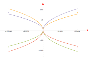
Fig. 8 : Solution of dispersion relation (19) for $a=10,G_{0}=25$ ; 4 different real roots are displayed by different color.

Fig. 9 : Plot for Alfvén Mach Numbers versus $k$ for: macro-scale vector-fields $M_{A}$ (top) and micro-scale vector-fields ${\tilde{M}_{A}}$ (bottom), respectively for generated velocity and magnetic fluctuations for the root 4 of Fig.8; $a=10>\sqrt{G_{0}}=5$. Bigger the $k$ smaller is $M_{A}$ but still $\ll 1$ ; micro scale fluctuations are Super-Alfvénic. $\alpha=10^{-6}$ .

Fig. 10 : Plot for Alfvén Mach Numbers versus $k$ for: macro-scale vector-fields $M_{A}$ (top) and micro-scale vector-fields ${\tilde{M}_{A}}$ (bottom), respectively for generated velocity and magnetic fluctuations for the root 8 of Fig.8; $a=10>\sqrt{G_{0}}=5$. Smaller the $k$ bigger is the $M_{A}$ that is $\gg 1$ while for micro-scale situation for Mach number reverses – Manifestation of Unified RD/Dynamo. $\alpha=10^{-6}$.

(2) For $a\sim 10\gg\sqrt{G}$, and ${\bf V}_{0}=\frac{a}{G}{\bf b}_{0}\ll{\bf b}_{0}$ – ambient flow is primarily magnetic. Dispersion relation is solved numerically and corresponding 8 real roots are displayed in Fig.8. In Fig.9 Alfvén Mach numbers for both the generated macro– and micro-fields are displayed for root 4. We observe, that the generated macro-scale flows are sub-Alfvénic while micro-scale flows are super-Alfveńic. This is the illustration of Unified Dynamo/RD scenario predicting strong magnetic field generation simultaneously to flows/outflows that are sub-Alfvénic. This, again, may explain the existence of strong magnetic fields in the vicinity of massive stars. Such scenario was absent in degenerate e-i case (see results of Section 2). The RD at short-scales for general settings was discussed in (Branderburg & Rempel, 2019). In Fig.10 Alfvén Mach numbers are plotted for root 8 for which we again observe a Unified RD/Dynamo process but now the generated macro-scale super-Alfvénic flow is very fast; short-scale fluctuations follow Dynamo process. According to (Beskin, 2010) $M_{A}\geq 10^{3}$ is observed in a variety of astrophysical outflows. It is remarkable that our result shows similar rate extremely fast flows for small $k$-s.

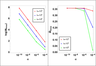
Fig. 11 : Maximal values of Alfvén Mach Numbers versus $\alpha$ for: macro-scale vector-fields $M_{Amax}$ (left) and micro-scale vector-fields ${\tilde{M}_{Amax}}$ (right), respectively for generated velocity and magnetic fluctuations (for the root 8 of Fig.8); $a=10>\sqrt{G_{0}}=5$. Smaller the $\alpha$ bigger is the $M_{Amax}$ that can reach values $\gg 10^{3}$ at small $k$ (see Eq. (20)). Red, blue, green colors correspond to: $k=10^{3},\ 10^{4},\ 10^{5}$, respectively. Smaller the $k$ bigger is $M_{Amax}$ for the same $\alpha$.

We have examined the dependence of final results on the dimensionless parameter $\alpha\ll 1$. Results presented in Fig.11 show that maximal macro-scale Alfvén Mach number $M_{Amax}$ increases when decreasing $\alpha$ and can reach the values $\sim 10^{8}$ for very small $\alpha\lesssim 10^{-10}$ at $k\lesssim 1000$. This result proves that generated outflow has dispersion with ${\mbox{\boldmath$U$}}({\mbox{\boldmath$r$}},t)$ macro-scale velocity field varying in space and time. Our detailed analysis shows that for smaller densities (hence, for weaker degeneracy level $G_{0}$) picture changes very slightly, maximal values of macro-scale outflow reduce a little, while maximal values of micro-scale outflow increase more significantly. Main result is the same – there is a fast flow/outflow formation in degenerate e-p plasma of astrophysical objects due to Unified Reverse Dynamo/Dynamo mechanism. We understand, that when heating as well as well wave processes are included in the dynamical process of acceleration final values may change according to additional channels of energy transformations.

Thus, analysis showed that for strongly degenerate e-p astrophysical plasma the Unified RD/Dynamo scenario is guaranteed for one of the roots of dispersion relation; depending on the range of Beltrami scales (helicities) of e-p fluids as well as density ($G_{0}$ - degeneracy level) the ratio between macro-scale velocity and magnetic fields may become different; similar conclusions can be drawn for micro-scale fields. At the end, there can be any mixture of macro– and micro– fields over the time. There will be conditions favorable for macro-scale super-Alfvénic flows to be generated together with the macro-scale magnetic fields and from these macro-scale solutions one can extract the density (degeneracy level) (see (Lingam & Mahajan, 2015) for details).

4 Conclusions

From an analysis of the degenerate two-fluid system, we have extracted the Unified Reverse Dynamo/Dynamo mechanism - the amplification/generation of fast macro-scale plasma flows in astrophysical systems with initial turbulent (micro–scale) magnetic/velocity fields. This process is simultaneous with and complementary to the micro-scale unified Dynamo/RD dynamics. It is found (both analytically and numerically) that like in the classical case the generation of macro–scale flows is an essential consequence of the magneto-fluid coupling. The generation of macro–scale fast flows and magnetic fields are simultaneous: the greater the macro–scale magnetic field (generated locally) the greater becomes the macro–scale velocity field (generated locally). Principle results of our investigation are following:

• The flow/outflow acceleration due to the Unified RD/Dynamo is directly proportional to the initial turbulent magnetic energy in degenerate e-i astrophysical plasma, while in degenerate e-p plasma such flows are fed by either initial turbulent state: kinetically or magnetically dominated ambient system; in the latter case generated/accelarated outflows are very strong.

• Depending on ambient density ($G_{0}(n)$) of degenerate two-fluid system the scenarios become different for different Beltrami parameter ($a$) but there always exists such a real $\omega$ (solution of dispersion relation) for which the generation of strong macro-scale fast locally Super-Alfvénic flow/outflow is guaranteed.

• Formation process is very sensitive to both the degeneracy state of the system and the magneto-fluid coupling. For the same parameters ($G_{0}$ and $a$), generated flow/outflow will have a dispersion with Velocity field distribution in (${\bf r},t$) – observations show that large-scale astrophysical flows are very complex with a characteristic evolution in time and space.

• It is interesting, that even the accelerated flows are sub-Alfvénic in some regimes for ambient system parameters, the flows, along with the dominant magnetic fields, will continue to amplify as long as there is an ambient turbulent energy to drive them – both fields grow at the rate defined by the dispersion relation (19) and determining parameters are $\alpha$ and $r$ (defined by (18)).

• In case of degenerate e-i plasma when the microscopic magnetic field is initially dominant, a major part of its energy transforms to super-fast super-Alfvénic macro–scale outflow energy due to magneto-fluid coupling; a weak macro–scale magnetic field is generated along with it. Specifically important finding is that in degenerate e-p plasma the whole set of cases may exist because of the different channels related to different real roots of dispersion relation, and for realistic physical parameters the resulting accelerated / generated locally super-Alfvénic flows are extremely fast with Alfvén Mach number $>10^{3}$ as observed in a variety of astrophysical outflows.

Thus, the unified Reverse Dynamo/Dynamo mechanism, providing an unfailing source for macro-scale fast flows/outflows becomes very significant together with other additional mechanisms (e.g. energy transformations due to catastrophe or waves) for understanding the existence of fast macro-scale flows/outflows in astrophysical objects with degenerate components – there is an intrinsic tendency of flow/magnetic field amplification due to magneto-fluid coupling in such system.

5 Acknowledgements

Authors express their thanks to Dr. Alexander Barnaveli for the valuable discussions. This work was supported by Shota Rustaveli Georgian National Foundation Grant Project No. FR17-391.

References

- Aksenov et al (2010) Aksenov, A.G., Ruffini, R. and Vereshchagin, G.V. Phys. Rev. E 81 046401 (2010).
- Arshilava et al. (2019) Arshilava, E. Gogilashvilia, M., Loladzea, V., Jokhadzea, I., Modrekiladzea, B., Shatashvilia, N.L. Tevzadze, A.G. J. High Energy Astrophysics 23, 6 (2019).