A non-linear mathematical model for the X-ray variability classes of the microquasar GRS 1915+105 - II: transition and swaying classes

Abstract

The complex time evolution in the X-ray light curves of the peculiar black hole binary GRS 1915+105 can be obtained as solutions of a non-linear system of ordinary differential equations derived form the Hindmarsch-Rose model and modified introducing an input function depending on time. In the first paper,assuming a constant input with a superposed white noise, we reproduced light curves of the classes $\rho$, $\chi$, and $\delta$. We use this mathematical model to reproduce light curves, including some interesting details, of other eight GRS 1915+105 variability classes either considering a variable input function or with small changes of the equation parameters. On the basis of this extended model and its equilibrium states, we can arrange most of the classes in three main types: $i$) stable equilibrium patterns (classes $\phi$, $\chi$, $\alpha^{\prime\prime}$, $\theta$, $\xi$, and $\omega$) whose light curve modulation follows the same time scale of the input function, because changes occur around stable equilibrium points; $ii$) unstable equilibrium patterns characterised by series of spikes (class $\rho$) originated by a limit cycle around an unstable equilibrium point; $iii$) transition pattern (classes $\delta$, $\gamma$, $\lambda$, $\kappa$ and $\alpha^{\prime}$), in which random changes of the input function induce transitions from stable to unstable regions originating either slow changes or spiking, and the occurrence of dips and red noise.
We present a possible physical interpretation of the model based on the similarity between an equilibrium curve and literature results obtained by numerical integrations of a slim disc equations.

1 Introduction

In a previous paper (Massaro et al., 2020, hereafter Paper I) we have shown that the complex time evolution of some variability classes exhibited by the peculiar Black Hole binary (BHB) GRS 1915+105 are obtained as solutions of a system of ordinary differential equations (ODEs). It is known that light curves of GRS 1915+105 in the X-ray band were classified in 14 different types, and it is possible that other new types can be introduced. The first classification was proposed by Belloni et al. (2000) who defined 12 variability classes on the basis of a large collection of multi-epoch RXTE observations. Two more classes were discovered in the following years (Klein-Wolt et al., 2002; Hannikainen et al., 2003, 2005)

The ODE system proposed in Paper I is based on the so-called Hindmarsh-Rose model (Hindmarsh & Rose, 1984; Hindmarsh & Cornelius, 2005), widely used in the description of neuronal behaviour. We introduced some changes with respect to the original formulation and refer to the new system as Modified Hindmarsh-Rose (MHR) model, that is non-autonomous because of the presence of an input function depending upon the time. We were thus able, assuming a constant input with a superposed white noise, to reproduce light curves of the classes $\phi$, $\chi$ and $\delta$, the last one characterized by a red noise Power Density Spectrum (PDS), and in particular those of the $\rho$ class limit cycle with its quasi regular series of spikes. An interesting finding was that the MHR model leads naturally to the onset of low frequency QPOs when the values of the input function vary in a transition range between unstable and stable equilibrium. As we wrote in Paper I this mathematical model should be considered as a useful tool for describing in a unified picture some non-linear effects occurring in the variability classes and their transitions.

In the present paper we will show that the MHR model can be used for reproducing X-ray light curves of several other variability classes of GRS 1915+105 either with an assumption of a variable input function or with small changes of the parameters. The success of this mathematical model is due to the fact that it appears a quite good analytical approximation of some instability conditions that can occur in accretion discs.

In Sections 2 and  3 we summarize the MHR model and extend it to the case of a new free parameter and a variable input function; in Section  4 show as this extended MHR model can account for light curves of the $\alpha^{\prime}$, $\gamma$ and $\kappa$ classes; in Section  5 we reproduce light curves of other variability classes which require rather ad hoc input functions, but, nevertheless, exhibit some minor interesting features; finally, in Section  6 we discuss some possible physical interpretation of the MHR model on the basis of some literature results obtained by numerical integrations of disc equations.

2 The MHR non-linear ODE system

The MHR model introduced in Paper I consists of two ODEs:

$$\frac{dx}{dt} = -\rho x^{3}+\beta_{1}x^{2}+y+J(t)$$

$$\frac{dy}{dt} = -\beta_{2}x^{2}-y$$ (1)

In Paper I the parameters where kept fixed to the values and $\beta_{1}=\beta_{2}=3.0$ and the input function $J(t)$ was taken in the form

$$J(t)=J_{0}+C~{}r$$ (2)

where $J_{0}$ is a constant, $r$ is a random number with a uniform distribution in the interval [$-0.5$, $0.5$], and a resulting standard deviation $\sigma_{J}=C/(2\sqrt{3})$ independent of the $J_{0}$ values, and $C$ is a constant factor to vary the amplitude of the random fluctuations.

In the present work we fixed again the value of $\rho=1.0$, without any loss of generality, because this is not an interesting parameter that can be eliminated by a simple change of variables as shown in Paper I, while in a few cases $\beta_{1}$ and $\beta_{2}$ were different; moreover we substitute $J_{0}$ with a variable $J_{S}(t)$, whose particular shape was adapted to reproduce light curves of the various classes. Thus, in place of Eq. (2) we write:

$$J(t)=J_{S}(t)+C~{}r$$ (3)

Numerical computations were again performed by means of a Runge-Kutta fourth order integration routine (Press et al., 2007), that was verified very stable and fast.

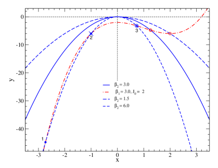
Figure 1: Nullclines for the system of Eq. 4 for $J_{0}=2.0$ and $\beta_{1}=3.0$ (red curve); the blue curves are the parabolas given by the second of Eq. 4 for different values of $\beta_{2}$. The open red circles are the equilibrium points of the two low $\beta_{2}$ parabolae, and the blue circles with numbers are the three equilibrium points for the high $\beta_{2}$ parabola. The cross and the large circle mark the saddle and unstable point, respectively.

3 Nullclines, equilibrium states and stability

In the case $J_{S}(t)=J_{0}$, the equilibrium conditions for the system of Eq. 1 with $\rho=1$, i.e. $\dot{x}=\dot{y}=0$, are

$$y = x^{3}-\beta_{1}~{}x^{2}-J_{0}$$

$$y = -\beta_{2}~{}x^{2}$$ (4)

thus the equilibrium points are the solutions of a cubic equation, as explained in the Appendix A. An interesting possibility is that of having three equilibrium points instead of only one, as in Paper I. A lower or a higher value of $\beta_{2}$ corresponds to a nullcline with a lower or a higher curvature, respectively. Fig. 1 shows some nullclines in the $x,y$ plane: we plotted only one cubic nullcline with $\beta_{1}=3.0$ $J_{0}=2.0$, typical values adopted in our computations, together with three parabolic nullclines. The solutions and the stability conditions are given in the Appendix A: the condition to have three equilibrium points is that $\beta_{2}>5.38$. In Fig. 1 we plotted two parabolas for low $\beta_{2}$ values with only one equilibrium point, while the third one has three intersections with the cubic one, marked by 1, 2, and 3. Using the linear analysis in the Appendix A it is easy to verify that: $i$) for $x_{*1}$ one has $\Delta>0$ and $Tr<0$ and the equilibrium is stable, $ii$) for $x_{*2}$, $\Delta<0$ and $Tr<0$ corresponding to a saddle point, and $iii$) for $x_{*3}$, $\Delta>0$ and the equilibrium can be either stable or unstable. The saddle point drives trajectories along the nullclines and prevents those moving away from them. It is remarkable that in the interval between $x_{*1}$ and $x_{*2}$ the two nullclines are very close to each other, a property relevant to understand the bursting process.

3.1 Variable $J_{S}(t)$

Several classes are characterised by flux variations on time scales longer than those of the $\rho$ self-oscillations. Such slow time scales are not intrinsic to the MHR model of Eq. 1 and can only be explained by means of a variable input function having values generally lower than the one necessary to develop the spiking behaviour. In this way the solutions of Eq. 1 are substantially driven by $J_{S}(t)$, that can be assumed to have rather simple profiles like a step (or multistep) function or a power law triangular profile, with an amplitude varying between 0 and 1:

$$J_{S}(t) = J_{m}\Big{[}1-\Big{(}1-\frac{t}{t_{1}}\Big{)}^{m}\Big{]}~{}~{}~{}~{},~{}~{}~{}0<t<t_{1}$$

$$J_{S}(t) = J_{m}\Big{(}\frac{1-t/T}{1-t_{1}/T}\Big{)}^{n}~{}~{}~{}~{}~{}~{}~{},~{}~{}~{}t_{1}<t<T$$ (5)

where $T$ is the duration (or period) of the modulation and $t_{1}$ is the time of the maximum amplitude $J_{m}$; $m$ and $n$ are real exponents that make curve the rising and decaying sections of this function ($m=n=1$ result in straight lines while for very high values they approximate well a square wave pattern). When it would be useful local and irregular features will also be considered to reproduce some details of the observed light curves.

4 Solutions with $\beta_{2}\neq\beta_{1}$

We verified that solutions of MHR model reproduce the light curves of some other classes with a satisfying accuracy if the condition $\beta_{1}=\beta_{2}$ is released. We decided, therefore, to keep $\beta_{1}$ fixed at 3.0, as in Paper I, and change only $\beta_{2}$. In particular, as shown in the following, the condition $\beta_{2}<\beta_{1}$ gives good curves for the $\kappa$ and $\gamma$ class, while $\beta_{2}>\beta_{1}$ is required for the $\alpha^{\prime}$ class.

We point out first that the criteria for the light curve classification of GRS 1915+105 used by Belloni et al. (2000) are not completely unambiguous and, looking at the individual light curves listed in that paper, one can notice different structures The classes $\alpha$, $\nu$ and $\beta$ exhibit similar patterns characterized by spike bursting patterns alternating with a smooth decline and a slower rise. The typical duration of the bursting phase is around 500 s, while the smooth interburst segments can be of the order of 1000 s and even longer. In the following, therefore, we distinguish two subclasses, here indicated as $\alpha^{\prime}$ and $\alpha^{\prime\prime}$ because their light curves have different structures despite being reported in the same class. According to the previous modelling the slow modulation is explained by variations of the input function $J(t)$, while the bursting is produced by the relaxation oscillation when the high value of $J$ leads the system to the unstable region.

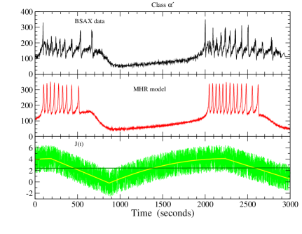
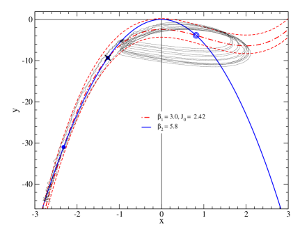
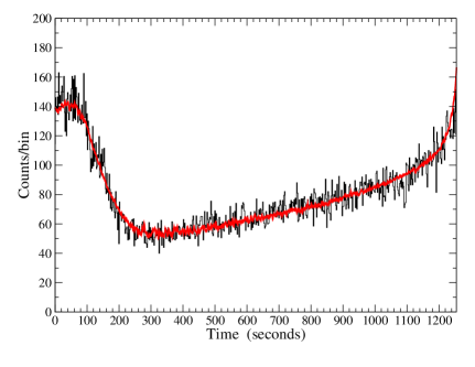
Figure 2: Top panel: top: short segment of MECS light curve of the $\alpha^{\prime}$ class; centre: a light curve (red) computed using the MHR model with the parameters’ values in Table 1; bottom: the input function $J(t)$ (green) with random fluctuations superposed onto a slowly variable modulation $J_{S}(t)$ (yellow); the dark green line is the mean value.
Central panel: the nullclines and the phase space trajectory (black) for the $\alpha^{\prime}$ class MHR solution; the thick red curve corresponds to the mean value of $J(t)$ and dashed ones are for the maximum and minimum values of $J_{S}(t)$;
Bottom panel: detail of the interburst segment with the model (red) superposed onto data (black); the time scale was adjusted to match the total duration.

4.1 $\beta_{2}>\beta_{1}$: class $\alpha^{\prime}$

An example of the $\alpha^{\prime}$ class light curve, observed with the MECS (Boella et al., 1997) on board the BeppoSAX satellite on 1995 November 11 in the energy range 1.5-10 keV is shown in the top panel in Fig.  2. It presents a short series of spikes, some of them similar to those of the $\rho_{d}$ class, with an increasing time separation between them; after the last spike the count rate decreases smoothly to the minimum level in about 200 s to increase again to a level at which the spiking activity starts again. We were able to reproduce the most characterizing features of this pattern (top panel centre) by assuming a value of $\beta_{2}$ above the three equilibrium points threshold (see Appendix A) together with a slowly modulated input function having a pattern resembling a sinusoidal oscillation (top panel bottom). For low values of $J_{S}(t)$ the system is in the stable interval and the solutions are mainly determined by the shape of the nullclines. When the value of $J_{S}(t)$ becomes high enough to move the system towards the unstable region the spikes appear and the subsequent decline is responsible of their increasing recurrence time; spikes cease when input function moves again to the stable region. It is worth noticing that the spiking behaviour is a consequence only of the system entering the unstable region and it is not specifically triggered by features in the $J(t)$ function.

Table 1: Parameters’ values adopted in the numerical calculations of the light curves for the various variability classes of GRS 1915+105.

Class	$\beta_{1}$	$\beta_{2}$	$C$	$J_{0}$	$J_{m}$	$\langle J\rangle$
$\alpha^{\prime}$	3.0	5.8	4.00	$-$0.2	4.30	2.420
$\gamma$	3.0	2.1	7.00	2.50	2.40	3.704
$\kappa$	3.0	1.6	6.00	$-$2.20	6.60	1.859
$\lambda$	4.0	4.0	5.00	1.45	0.00	$-$2.515
$\omega$	3.0	3.0	4.50	$-$2.30	1.20	$-$0.348
$\alpha^{\prime\prime}$	3.0	3.0	10.5	$-$6.70	1.30	$-$0.797
$\xi$	3.0	3.0	7.00	$-$2.70	2.81	$-$1.137
$\theta$	3.0	3.0	4.50	$-$3.20	2.20	$-$2.475

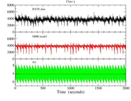
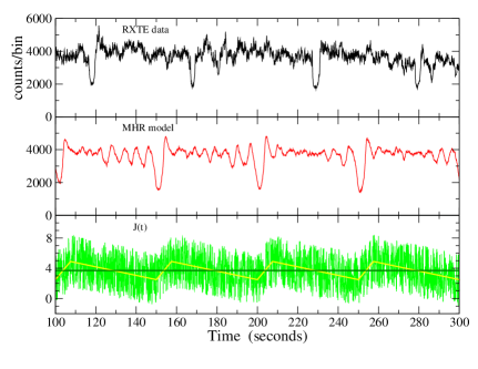
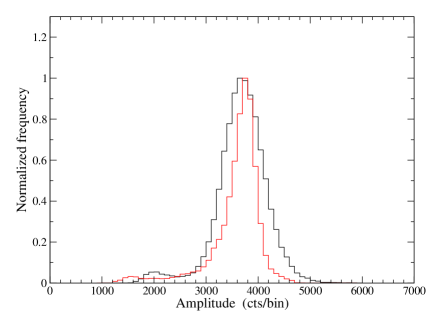
Figure 3: Top panel: segment of RXTE light curve of the $\gamma$ class (ID 20402-01-39-00); centre with a bin size of 0.125 s; a light curve (red) computed using the MHR model using the parameters’ values in Table 1; the input function $J(t)$ (green), with random fluctuations superposed onto an oscillating function $J_{S}(t)$ (yellow curve) with the same time scale of dip recurrence.
Central panel: zoom-in of the time series plotted in the top panel to compare their structures on short time scales.
Bottom panel: histograms of the amplitude distributions in the real data (black) and computed series (red), normalized to unity at the maxima to compare their asymmetric profiles.

As shown in the phase space plot (black dashed line in the central panel in Fig. 2), in the stable region the trajectory is practically confined in a narrow channel between the two nullclines (Hindmarsh & Rose, 1984; Hindmarsh & Cornelius, 2005). We plotted here three cubic nullclines: the central and solid line was computed assuming $J_{0}=\langle J(t)\rangle$, while the other (dashed) two correspond to the extreme values of $J_{S}(t)$, namely 4.2 and $-$0.2. This portion of the trajectory depends upon the existence of a saddle point between the stable and unstable states and explains the shape of the non-spiking segment. Its evolution is governed by the decay and increasing time scales of $J_{S}(t)$, while the detailed shape is given by the polynomial nullcline profiles and it is remarkably similar between the various bursts (bottom panel in Fig. 2). Not, in particular, that its curvature is opposite to that of $J_{S}(t)$. Then the trajectory moves into the unstable region and the system changes to the spiking behaviour that corresponds to the winding loops. Finally, note that the lowest $x$ points in the loops are very close to the saddle point, and this explains the change of direction of the trajectory toward the stable channel.

As shown in Paper I, a very interesting property of the $\rho$ class spikes is that their recurrence time depends upon the local mean value of $J_{S}(t)$. In particular a decreasing $J$ corresponds to an increase of the recurrence time, and when it becomes lower than the stability threshold the spiking behaviour is quenched. A bursting pattern like that of this class was obtained in early works on the original HR model (see, for instance, Shilnikov & Kolomiets 2008) in which an oscillating solution for $J(t)$ is obtained from the third ODE in Eq. 1 in Paper I. Such a complete system is autonomous and gives also all the solutions described in Paper I. In particular, the equation for the derivative of $J_{S}(t)$ depends upon $x$ and $J$, but it contains three more parameters. However, it is hard to obtain solutions with more complex changes and very high gradients as those used in the following sections and therefore we preferred to consider this function as an independent input.

4.2 $\beta_{2}<\beta_{1}$: class $\gamma$

Light curves of the $\gamma$ class are characterized by a rather stable count rate resembling the $\chi$ or $\delta$ class, with superposed several narrow spikes and narrow dips with a time separation of a few tens of seconds (Fig. 3, top). Despite its apparent simplicity these data are not reproduced by means of a constant $J_{S}(t)$ and require a more elaborated model with a a rapidly oscillating function having the duration of the cycles close to the separation time between the dips (Fig. 3, bottom) and a mean value inside the instability range but with an amplitude large enough to reach the upper stability domain. In our calculations we adopted $\beta_{1}=3.0$ as in the previous cases, but fully satisfactory results are also obtained adopting values of $\beta_{1}$ and $\beta_{2}$ lower than 3.0 because, the unstable interval is rather narrow and rather small changes of $J_{S}(t)$ are enough to produce a transition between the two regimes.

A model light curve is given in the top panel of Fig. 3 (centre), and it reproduces many features of the observed curve, in particular the presence of recurrent dips. The model is able to match the data behaviour on time scales as shorth as 10 s, as shown by the two light curve segments in the central panel in Fig. 3. Note that the amplitude distribution of spikes and dips is asymmetric because the latter ones have a typical amplitude higher than spikes. If one computes the histogram of the amplitude values can verify that it is left asymmetric; the same property is also present in the histogram of model light curve (bottom panel in Fig. 3), although the properties of the noise are not the same as the source.

4.3 $\beta_{2}<\beta_{1}$: class $\kappa$

This is a peculiar class because light curves exhibit a large variety of patterns: also the RXTE observations reported by Belloni et al. (2000) are largely uneven. We decided to consider here an observation performed on 1997 June 18 (ID P20402-01-33-00). The structure of this light curve is characterized by large bursts (their typical widths range from $\sim$100 s to more than 200 s) with very fast rise and decay; narrow spikes frequently occur at the maximum of the rising portion or during the decay, as shown in the top panel in Fig. 4. The MHR model works nicely when $\beta_{1}>\beta_{2}$, that in our case are equal to 3.0 and 1.6, respectively. The input function $J(t)$, shown in the bottom panel of Fig. 4, is rather similar to that of the $\gamma$ class with a simple oscillating square profile but with a quite lower mean value; the recurrence time of major bursts was reduced in the second part of series to make the numerical results more similar to the observed data. Note that the mean value of these oscillations varies between the stable (at the minimum level) and the unstable (at the maximum level) ranges.

The MHR model reproduces not only the typical burst profiles but also some details as the fast spikes at the end of the rise and the other one in the decay, without any ad hoc additional feature in the $J_{S}(t)$ function. These features are indeed related to the fast transitions segments which can trigger the onset of a spike mode, soon damped by the fast change of $J_{S}(t)$. Clearly, the occurrence of other minor structures in the input function could produce more complex features in the resulting light curves.

It is interesting that one of the light curves computed by Janiuk et al. (2002) for a disk model with a radiative instability has $\kappa$-like bursts with similar spikes. This model was computed for a central black hole of 10 $M_{\odot}$, comparable to the one estimated for GRS 1915+105, with about 1/3 of the energy dissipated in the corona and an outflow, i.e. with additional dissipation processes. Unfortunately, details of this model and an interpretation of the causes of these burstings are not given and a comparison of these finding with ours is not possible.

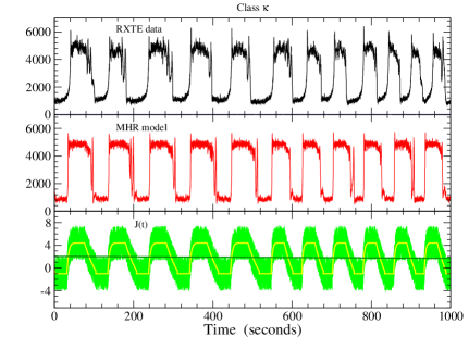
Figure 4: Top panel: segment of RXTE light curve of the $\kappa$ class (ID 20402-01-33-00). Central panel: a light curve (red) computed using the MHR model using the parameters’ values in Table 1. Bottom panel: the input function $J(t)$ (green), with random fluctuations superposed onto an oscillating pattern ($J_{S}(t)$, yellow line) and its mean value (dark green line).

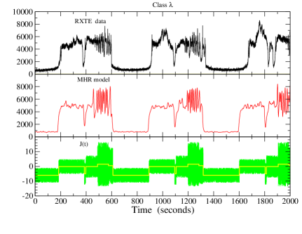
Figure 5: Top panel: short segment of RXTE light curve of the $\lambda$ class (ID 20402-01-37-01) Central panel: a light curve (red) computed using the MHR model using the parameters’ values in Table 1. The noise is reduced because a running average was applied to this series to have a time resolution comparable to those of the data. Bottom panel: the input function $J(t)$ (green), with random fluctuations superposed onto a slowly changing step function with abrupt interruption ($J_{S}(t)$, yellow curve).

5 Solutions with $\beta_{1}=\beta_{2}$

Our numerical calculations showed that the simple MHR system proposed in Paper I is also able to reproduce the main features of several other variability classes, but with the two following assumptions: $i$) the values of the input function satisfy the condition that the equilibrium point remains in the stable region, $ii$) the changes of the input function must be over time scales similar to those in the observed light curves.

We considered two typical rather simple structures for $J_{S}(t)$: $i$) a series of step functions, repeating the same pattern with a recurrence time as the one found in the individual data series; $ii$) a combination of slowly modulated variation and step functions, when necessary. The discussion of a specific physical explanation of these time structures is beyond the purpose of this paper. However, assuming they are related to the local mass accretion rate, this assumption requires the occurrence of particular modulations.

Considering that we are working mainly in stable equilibrium conditions we adopted $\beta=3.0$ as in Paper I. Some values of the parameters of $J_{S}(t)$ used in numerical calculations are given in Table 1.

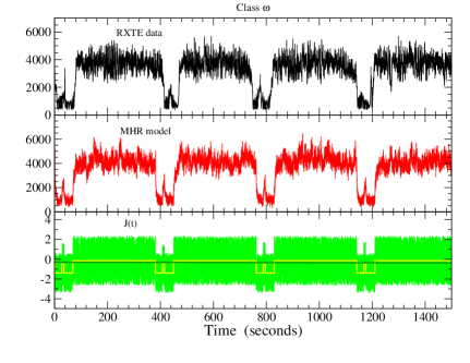
Figure 6: Top panel: short segment of RXTE light curve of the $\omega$ class (ID 40703-01-27-00). Central panel: a light curve (red) computed using the MHR model using the parameters’ values in Table 1. Bottom panel: the input function $J(t)$ (green), with random fluctuations superposed onto a slowly changing function with abrupt interruption ($J_{S}(t)$, yellow line).

5.1 Class $\lambda$

This is one of the original classes by Belloni et al. (2000), characterised by a complex pattern consisting of rather long bursts with an initial segment similar to the $\delta$ class followed by a series of fast oscillations. In the calculation we adopted the choice $\beta_{1}=\beta_{2}=4.0$, instead of the canonical 3.0, but very good solutions are also obtained with $\beta_{1}>\beta_{2}=3.0$. According to the input function models described in Sect. 3.1, we used a three/four level step function (see the bottom panel in Fig. 5): the lowest level corresponds to the minimum steady flux, while of the two higher levels, the one below the zero produces the $\delta$ segment and the positive one the fast oscillating, respectively. A fourth level was introduced to have a smooth decline with an increasing recurrence time between oscillations. Moreover, a dip was included in the second segment to obtain a more faithful correspondence with the observed signal, but this feature is not always necessary because not present in other $\lambda$ data series. The resulting light curve is shown in Fig. 5; original results exhibit high amplitude fast oscillations and were smoothed applying a running average algorithm to make them comparable with data.

5.2 Class $\omega$

One of the simplest classes to reproduce is the $\omega$ class, that was recognized by Klein-Wolt et al. (2002) and presents rapidly fluctuations with respect to a rather stable level having a duration around 300 s, interrupted by low intensity intervals, typically shorter by 80-100 s, and occasionally with a spike in the middle.

We obtained numerical results similar to this class by means of a $J_{S}(t)$ having a three level square wave modulation as shown in the bottom panel in Fig. 6.

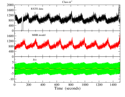
Figure 7: Top panel: segment of RXTE light curve of the $\alpha^{\prime\prime}$ class (ID 20402-01-22-00). Central panel: a light curve (red) computed using the MHR model using the parameters’ values in Table 1. Bottom panel: the input function $J(t)$ (green), with random fluctuations superposed onto a sawtooth law with $t_{1}/T=0.80$; the yellow line is the $J_{S}(t)$ function, and the dark green line corresponds to its mean value.

5.3 Class $\alpha^{\prime\prime}$

As writte above, light curves of the Belloni et al. (2000) $\alpha$ class have different time structures. Here we considered the observation ID 20402-01-22-00 with rather smooth variation, resembling a sawtooth profile, with a recurrence time of about 150 - 200 s, remarkably different from the $\alpha^{\prime}$ profile, and that for this reason we report here as $\alpha^{\prime\prime}$. The MHR model reproduces this class by assuming a sawtooth profile for $J_{S}(t)$ and a high statistical noise superposed onto it (see Fig. 7): note that when the $J(t)$ is close to the maxima, a few small amplitude spike can be present, as in the real data.

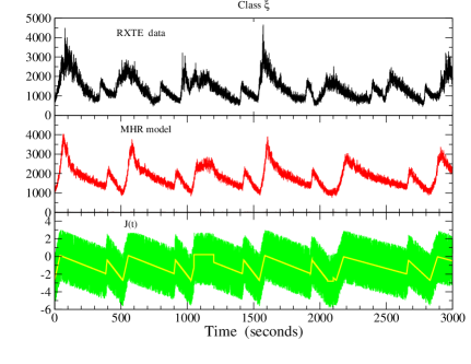
Figure 8: Top panel: short segment of RXTE light curve of the $\xi$ class (ID 80127-01-02-01). Central panel: a light curve (red) computed using the MHR model using the parameters’ values in Table 1. Bottom panel: the input function $J(t)$ (green), with random fluctuations superposed onto a slowly changing function with abrupt interruption, the yellow line corresponds to $J_{S}(t)$.

5.4 Class $\xi$

This class was firstly reported by Hannikainen et al. (2005): it consists of a triangular modulation characterised by a rise portion shorter than the decaying one, at variance with the shape of typical $\rho$ burst. It looks rather similar to a time reversed $\alpha^{\prime\prime}$ class. Duration and height of these triangles are quite variable; the former ones range from $\sim$100 s to more than $\sim$300 s, and the amplitude ratio can be as high as a factor by about 4 (see Fig. 8). We considered a $J_{S}(t)$ function given by the superposition of two sawtooth of different amplitudes and added some changes to have a result similar to the observed light curve, as an increase of the sawtooth duration and a flat segment in correspondence of the third peak. What is important is that the mean signal remained below the zero level, that is nearly coincident to the instability threshold. When, in correspondence to the sawtooth maxima, this threshold is occasionally exceeded, some narrow spikes are obtained.

5.5 Class $\theta$

This class was defined by Belloni et al. (2000) and was characterized by cycles over a time scale of about 1000 s, with a nearly triangular modulation interrupted around the maximum by a low count rate intervals having a duration of 100-300 s and occasionally one or more spikes in the middle. The MHR model reproduces these features if the slow modulation is present in the $J_{S}(t)$, as shown in the central and bottom panel in Fig. 9.

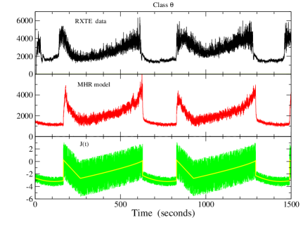
Figure 9: Top panel: short segment of RXTE light curve of the $\theta$ class (ID 10408-01-15-04). Central panel: a light curve (red) computed using the MHR model using the parameters’ values in Table 1. Bottom panel: the input function $J(t)$ (green), with random fluctuations superposed onto a slowly changing function with abrupt interruption, the yellow line is the $J_{S}(t)$ the function.

6 Summary and discussion

The results presented in this paper, together with those in Paper I, show that the MHR mathematical model is a useful and powerful approximation to describe the non-linear processes occurring in the plasma of an accretion disc and originating several complex patterns of luminosity variations. It is, therefore, a promising tool for describing the equilibrium conditions of the plasma states and for the physical modelling of disc instabilities. Moreover, the MHR model can help in the understanding of the evolution of local instabilities originating the various light curve structures. Furthermore, as shown in Paper I, the model suggests a new mechanism for the origin of QPOs in the Hz region.

Our calculations have shown that several variability classes of GRS 1915+105 are obtained by changing only the input function $J(t)$. These variations can produce transitions between stable and unstable states, and using this property we can group the variability classes into the following three main types:

$i$) stable equilibrium patterns: this group includes the classes $\phi$, $\chi$, $\alpha^{\prime\prime}$, $\theta$, $\xi$, and $\omega$, corresponding to variations around the nullcline determined by the position of a stable equilibrium with the light curve modulated with the same time scale of the changes of $J_{S}(t)$;

$ii$) unstable equilibrium (spiking) patterns: typically characterized by long series of spikes like the $\rho$ (and $\rho_{d}$) class, it is originated when $J(t)$ becomes high enough to move the equilibrium point within the instability interval; spikes are a recurrence time depending upon the mean level of the $J(t)$ and decrease when this value increases;

$iii$) transition (bursting) patterns: this group includes the classes $\delta$, $\gamma$, $\lambda$, $\kappa$ and $\alpha^{\prime}$, in which the variations of $J(t)$ produce transitions from stable to unstable regions (and vice versa), thus originating either smooth changes or spiking, and occasionally the occurrence of dips and red noise; the $\rho_{d}$ subclass should be classified in this type because of the highly irregular recurrence of spikes and the occurrence of plateau between them, which can be due $J$ fluctuations across the stability boundary.

There are other criteria for grouping the variability classes. For instance Misra et al. (2004) and Misra et al. (2006), on the basis of a search for a chaotic behaviour, defined the following three groups: non-linear deterministic or chaotic classes ($\theta$, $\rho$, $\delta$, $\alpha^{\prime}$, $\alpha^{\prime\prime}$), purely stochastic classes ($\phi$, $\chi$, $\gamma$), and a mix of stochastic and chaotic ($\beta$, $\lambda$, $\mu$, $\kappa$). These groups are different from ours because their classification criteria are based on the estimate of the correlation dimension and are not very efficient for distinguishing the non-stochastic variations in light curves like those of the $\gamma$ or $\kappa$ classes,

One of the advantages of the MHR model is in its simplicity. As already pointed out in Paper I, we recall that the model describes only time changes of the luminosity without considering how these depend upon the energy. The extension of the model, if possible, would likely require at least a new non-linear equation and/or the addition of new terms and parameters which would make quite difficult the stability analysis of solutions and the conditions for the occurrence of a limit cycle.

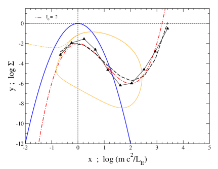
Figure 10: Nullclines of the MHR model of Eqs.(4) for $\beta_{1}=3$ and $J(t)=J_{0}=2$ (thick red curve) and the solid blue curve is the parabola for $\beta_{2}=3$. The red circle marks the unstable equilibrium point. Black triangles are the values computed by Watarai & Mineshige (2001) for a slim disk for the logarithms of mass accretion rate in the abscissa and that of the disk surface density in the ordinate. These values were scaled to those of our variables to approximately match the curves and dashed black curve is a cubic best fit. The orange line is the same limit cycle for the $\rho$ class discussed in Paper I.

We now consider a possible physical interpretation of the MHR model and of the nature of the input function $J(t)$. In the previous paper concerning the FitzHugh-Nagumo model, Massaro et al. (2014) proposed that it could be related to the mass accretion rate in the disc. This hypothesis was suggested by the fact that this ’external’ parameter rules the disc luminosity, but the actual dependence of $J(t)$ from mass accretion rate cannot be easily deduced from the data. It is not, however, the only interesting quantity and here we try to extend the analysis to other physical parameters on the basis of the results of some theoretical studies.

One can reasonably rise the question why such complicated dynamical processes are captured by a rather simple non-linear ODE system. There is no simple answer, but a possible indication is that the equilibrium conditions for the plasma can be approximated by polinomial functions, at least within the limited interval around the unstable states, as those used in the MHR model. This property is found to be common to many physical systems exhibiting self oscillations (see Jenkins (2013), for a clear introduction), including the macroscopic behaviour of Cepheids variable stars, whose non linearity is gathered by the period-luminosity relation. We recall that also for GRS 1915+105 Massaro et al. (2010) reported that the mean recurrence time of $\rho$ bursts is positevely correlated with the average count rate, indicating the occurrence of a similar relation.

Researches on instabilities in accretion disks started in the seventies (e.g. Lightman & Eardley, 1974; Pringle et al., 1973; Shakura & Sunyaev, 1976) and up to now an extensive literature has been produced. Taam & Lin (1984), in particular, computed by means of numerical integration of the non-linear disk equations, applying the $\alpha$ prescription for the viscosity (Shakura & Sunyaev, 1973) to investigate thermal-viscous instabilities and obtained theoretical light curves having recurrent flares. With the discovery of the $\rho$ class variability in GRS 1915+105, Taam et al. (1997) investigated the time and spectral properties of the bursts and proposed an interpretation based on the instability discussed in the previous paper. The evolution of thermal-viscous instabilities in an accretion disc was associated with a limit cycle (e.g. see Szuszkiewicz & Miller, 1998), generally described by means of an S-shaped equilibrium curve in a plot of temperature or accretion rate vs disk surface density as shown by Abramowicz et al. (1995). Other equilibrium curves were computed in a model developed by Watarai & Mineshige (2001) and Mineshige & Watarai (2005) for a slim-disc (Abramowicz et al., 1988) as resulting from spectral analyses of GRS 1915+105 (Vierdayanti et al., 2010; Mineo et al., 2012).

Watarai & Mineshige (2001) computed the equilibrium relation in the plane $log(\dot{m}c^{2}/L_{E}),log(\Sigma)$ at a radial distance of 7 Schwarzschild radii, where $L_{E}$ is the Eddington luminosity and $\Sigma$ the surface density of the disc, and resulted an S-shaped pattern. These curves translate along the $log(\Sigma)$ axis with only small changes of the shape when the viscosity parameter $\alpha$ changes: $log\Sigma$ increases by a factor of about 40 when $\alpha$ decreases from 1.0 to 0.01. The S-profile becomes shallower and shallower for increasing values of the other parameter $\mu$, which measures the fractional relevance of the gas pressure to the viscous shear tensor:

$$\tau_{r\phi}=-\alpha P_{gas}^{\mu}P_{total}^{1-\mu}~{}~{}~{},~{}~{}~{}0\leq\mu\leq 1.$$ (6)

The structure of these curves is remarkably similar to that of the $\dot{x}$ cubic nullcline of MHR model as apparent in Fig. 10 where we reported one of the Watarai & Mineshige (2001) curves, precisely the one corresponding to $\mu=0$ and $\alpha=0.1$, scaled and translated to match the values used in our calculations and found a remarkable similarity with the nullcline. For a complete correspondence between these theoretical results and the MHR model we need the other relation between $log(\Sigma)$ and $log(\dot{m})$ related to the $\dot{y}$ ODE and with equilibrium conditions approximating the quadratic nullcline in order to have three equilibrium points necessary for the bursting pattern and the interburst profile of the $\alpha^{\prime}$ class. It will be useful to verify by means of numerical integrations of slim-disc equations if the solutions for physical variables, like the pressure or the temperature of the plasma, and consequently the viscous dissipation, follow a similar evolution during the limit cycle.

It is also interesting to note that the parameter $\mu$ affects the shape of the Watarai & Mineshige curves and therefore it works as the parameter ratio $\beta/\rho$ but in the opposite way. As for example, assuming a simple linear relationship between these two quantities one can write $\beta=k(1-\mu)$, thus $\mu=0$ corresponding to the most pronounced S-shape (in our case $k=3.0$). The existence of such a relation, however, requires many other calculations to be verified.

Another interesting possibility to obtain fast changes of $\alpha$ is the one proposed by (Potter & Balbus, 2014), who investigated the disc instability induced by the dependence of this parameter on the magnetic Prandl number, $Pm$, that is the ratio of the plasma (microscopic) viscosity to resistivity. Potter & Balbus (2017), using the PLUTO MHD numerical code (Mignone et al., 2007), demonstrated that the $\alpha-Pm$ dependence can be sufficiently strong to produce a local instability, which originates a limit cycle by mapping the S-shaped thermal-equilibrium curve of the disc. One can therefore expect that these variations could be the underlying mechanism originating $J_{S}(t)$.

A relevant issue is the definition of the physical meaning of the input function $J(t)$ and of the nature of its variations. In this work we adopted rather simple functions to define the main time scale useful for computing light curves in a fine similarity to the data, and obtained that they were not only in agreement with the general time structure but also in several details like, for instance, the spikes of the $\kappa$ class bursts. The historic light curve of GRS 1915+105 presents luminosity changes higher than one order of magnitude (Ghosh & Chakrabarti, 2018; Miller et al., 2019), which cannot be explained without large changes of an externally driven accretion rate. A consistent and complete modelling of this activity appears a goal quite hard to be achieved, in particular because many important informations are unknown, such as the modulation of the gas flow from the companion star.

Finally, we mention that a model for the $\rho$ class was proposed by Neilsen et al. (2012), who interpreted the bursting as a consequence of oscillations in the mass accretion rate. This hypothesis remains useful also in the context of the MHR model, but not, however, in the specific case of the $\rho$ spikes, but for the $\kappa$ and $\gamma$ class that require an oscillating $J_{S}(t)$ with the same time scale of the bursts or dips, respectively. Using this approach one should search for possible correlations between the properties of the various variability classes and the mean luminosity or other spectral parameters. This draining work is beyond the goals of the present paper that is focused on the development of a tool for describing the stability conditions through a single model that produce the rich collection of variability classes.

Appendix A Nullclines and equilibrium points for $\beta_{1}\neq\beta_{2}$

To study the solutions when $\beta_{1}\neq\beta_{2}$, we assume that $\beta_{1}$ is fixed to 3, while $\beta_{2}$ is variable with the condition to be always positive. Thus the nullcline for $\dot{x}$ remains equal to that shown in Fig. 1, while the value of $\beta_{2}$ determine the parabolic shape of the $\dot{y}$ nullcline. The equilibrium points with $J_{0}>0$ are thus given by the solution of the cubic equation:

$$x^{3}+(\beta_{2}-\beta_{1})x^{2}-J_{0}=0$$

For $\beta_{2}<3$ the curvature of the parabola is lower than that in Fig. 1 and there is only one real solution, while for $\beta_{2}>3$ it is possible to have three real solutions. The condition on $\beta_{2}$ is easily obtained after the reduction of the cubic equation to the canonical form

$$u^{3}+3pu-2q=0$$

where

$u=x+(\beta_{2}-\beta_{1})/3$   ,   $p=-(\beta_{2}-\beta_{1})^{2}/9$   ,
$q=(\beta_{2}-\beta_{1})^{3}/27+J_{0}/2$.

There are three real solutions if the discriminant satisfies the condition:

$$q^{2}+p^{3}<0$$

which implies the condition:

$$\beta_{2}$>$\beta_{1}+3(J_{0}/4)^{1/3}~{}~{},~{}~{}J_{0}>0$$

In the case considered in Section  3, that is $\beta_{1}=3.0$ and $J_{0}=2.0$, we have three real solutions when $\beta_{2}>3(1+2^{-1/3})=5.3811...$.

Let $x_{*}$, $y_{*}$ the equilibrium solution, the Jacobian computed at this point is:

$$\left(\begin{array}[]{cc}-3x_{*}^{2}+2\beta_{1}x_{*}&1\\ -2\beta_{2}x_{*}&-1\end{array}\right)$$

and its determinant and trace are:

$$\Delta=3x_{*}^{2}+2(\beta_{2}-\beta_{1})x_{*}~{}~{}~{}~{},$$

$$Tr=-3x_{*}^{2}+2\beta_{1}x_{*}-1~{}~{}~{}~{}.$$

The sign of $\Delta$ depends upon $\beta_{1}$ and $\beta_{2}$: for $\beta_{1}<\beta_{2}$ we have that $\Delta>0$ when $x_{*}<2(\beta_{1}-\beta_{2})/3$ or $x_{*}>0$, while for $\beta_{1}>\beta_{2}$ we have that $\Delta>0$ when $x_{*}<0$ or $x_{*}>2(\beta_{1}-\beta_{2})/3$. The trace is $Tr>0$ only for $(\beta_{1}-\sqrt{\beta_{1}^{2}-3}~{})/3<x_{*}<(\beta_{1}+\sqrt{\beta_{1}^{2}-3}~{})/3$ and negative outside this interval.

References

- Abramowicz et al. (1988) Abramowicz M. A., Czerny B., Lasota J. P., Szuszkiewicz E., 1988, ApJ, 332, 646
- Abramowicz et al. (1995) Abramowicz M. A., Chen X., Kato S., Lasota J.-P., Regev O., 1995, ApJ, 438, L37
- Belloni et al. (2000) Belloni T., Klein-Wolt M., Méndez M., van der Klis M., van Paradijs J., 2000, A&A, 355, 271
- Boella et al. (1997) Boella G., et al., 1997, A&AS, 122, 327
- Ghosh & Chakrabarti (2018) Ghosh A., Chakrabarti S. K., 2018, MNRAS, 479, 1210
- Hannikainen et al. (2003) Hannikainen D. C., et al., 2003, A&A, 411, L415
- Hannikainen et al. (2005) Hannikainen D. C., et al., 2005, A&A, 435, 995
- Hindmarsh & Cornelius (2005) Hindmarsh J. L., Cornelius P., 2005, 2005, BURSTING: The Genesis of Rhythm in the Nervous System. S. Coombes & P.C. Bressloff eds
- Hindmarsh & Rose (1984) Hindmarsh J. L., Rose R. M., 1984, Proceedings of the Royal Society of London Series B, 221, 87
- Janiuk et al. (2002) Janiuk A., Czerny B., Siemiginowska A., 2002, ApJ, 576, 908
- Jenkins (2013) Jenkins A., 2013, Phys. Rep., 525, 167
- Klein-Wolt et al. (2002) Klein-Wolt M., Fender R. P., Pooley G. G., Belloni T., Migliari S., Morgan E. H., van der Klis M., 2002, MNRAS, 331, 745
- Lightman & Eardley (1974) Lightman A. P., Eardley D. M., 1974, ApJ, 187, L1
- Massaro et al. (2010) Massaro E., Ventura G., Massa F., Feroci M., Mineo T., Cusumano G., Casella P., Belloni T., 2010, A&A, 513, A21+
- Massaro et al. (2014) Massaro E., Ardito A., Ricciardi P., Massa F., Mineo T., D’Aì A., 2014, Ap&SS, 352, 699
- Massaro et al. (2020) Massaro E. Capitanio F., Feroci M., Mineo T., Ardito A., Ricciardi P., 2020, MNRAS, submitted
- Mignone et al. (2007) Mignone A., Bodo G., Massaglia S., Matsakos T., Tesileanu O., Zanni C., Ferrari A., 2007, ApJS, 170, 228
- Miller et al. (2019) Miller J. M., Balakrishnan M., Reynolds M. T., Trueba N., Zoghbi A., Kaastra J., Kallman T., Proga D., 2019, The Astronomer’s Telegram, 12743, 1
- Mineo et al. (2012) Mineo T., et al., 2012, A&A, 537, A18
- Mineshige & Watarai (2005) Mineshige S., Watarai K.-Y., 2005, Chinese Journal of Astronomy and Astrophysics Supplement, 5, 49
- Misra et al. (2004) Misra R., Harikrishnan K. P., Mukhopadhyay B., Ambika G., Kembhavi A. K., 2004, ApJ, 609, 313
- Misra et al. (2006) Misra R., Harikrishnan K. P., Ambika G., Kembhavi A. K., 2006, ApJ, 643, 1114
- Neilsen et al. (2012) Neilsen J., Remillard R. A., Lee J. C., 2012, ApJ, 750, 71
- Potter & Balbus (2014) Potter W. J., Balbus S. A., 2014, MNRAS, 441, 681
- Potter & Balbus (2017) Potter W. J., Balbus S. A., 2017, MNRAS, 472, 3021
- Press et al. (2007) Press W. H., Teukolsky S. ., Vetterling W. T., Flannery B. P., 2007, Numerical Recipes: The Art of Scientific Computing, 3 edn. Cambridge University Press
- Pringle et al. (1973) Pringle J. E., Rees M. J., Pacholczyk A. G., 1973, A&A, 29, 179
- Shakura & Sunyaev (1973) Shakura N. I., Sunyaev R. A., 1973, A&A, 500, 33
- Shakura & Sunyaev (1976) Shakura N. I., Sunyaev R. A., 1976, MNRAS, 175, 613
- Shilnikov & Kolomiets (2008) Shilnikov A., Kolomiets M., 2008, International Journal of Bifurcation and Chaos, 18, 2141
- Szuszkiewicz & Miller (1998) Szuszkiewicz E., Miller J. C., 1998, MNRAS, 298, 888
- Taam & Lin (1984) Taam R. E., Lin D. N. C., 1984, ApJ, 287, 761
- Taam et al. (1997) Taam R. E., Chen X., Swank J. H., 1997, ApJ, 485, L83
- Vierdayanti et al. (2010) Vierdayanti K., Mineshige S., Ueda Y., 2010, PASJ, 62, 239