Millimeter- and submillimeter-wave spectroscopy of thioformamide and interstellar search toward Sgr B2(N)

Abstract

Context. Thioformamide NH2CHS is a sulfur-bearing analog of formamide NH2CHO. The latter was detected in the interstellar medium back in the 1970s. Most of the sulfur-containing molecules detected in the interstellar medium are analogs of corresponding oxygen-containing compounds. Therefore, thioformamide is an interesting candidate for a search in the interstellar medium.

Aims. A previous study of the rotational spectrum of thioformamide was limited to frequencies below 70 GHz and to transitions with $J\leq 3$. The aim of this study is to provide accurate spectroscopic parameters and rotational transition frequencies for thioformamide to enable astronomical searches for this molecule using radio telescope arrays at millimeter wavelengths.

Methods. The rotational spectrum of thioformamide was measured and analyzed in the frequency range 150 to 660 GHz using the Lille spectrometer. We searched for thioformamide toward the high-mass star-forming region Sagittarius (Sgr) B2(N) using the ReMoCA spectral line survey carried out with the Atacama Large Millimeter/submillimeter Array (ALMA).

Results. Accurate rigid rotor and centrifugal distortion constants were obtained from the analysis of the ground state of parent, ³⁴S, ¹³C, and ¹⁵N singly substituted isotopic species of thioformamide. In addition, for the parent isotopolog, the lowest two excited vibrational states, $\varv_{12}=1$ and $\varv_{9}=1,$ were analyzed using a model that takes Coriolis coupling into account. Thioformamide was not detected toward the hot cores Sgr B2(N1S) and Sgr B2(N2). The sensitive upper limits indicate that thioformamide is nearly three orders of magnitude at least less abundant than formamide. This is markedly different from methanethiol, which is only about two orders of magnitude less abundant than methanol in both sources.

Conclusions. The different behavior shown by methanethiol versus thioformamide may be caused by the preferential formation of the latter (on grains) at late times and low temperatures, when CS abundances are depressed. This reduces the thioformamide-to-formamide ratio, because the HCS radical is not as readily available under these conditions.

1 Introduction

Several small sulfur compounds have recently been observed in the interstellar medium (ISM): HS2 (Fuente et al., 2017), NS+ (Cernicharo et al., 2018), HCS, and HSC (Agúndez et al., 2018). To date, 23 sulfur derivatives have been detected or tentatively detected in the ISM, which means that the sulfur atom holds the fifth position after hydrogen, carbon, oxygen, and nitrogen atoms; see, for instance “Molecules in Space” in the Cologne Database for Molecular Spectroscopy. While the first four elements are represented in molecules ranging from 2 to 13 atoms with the exception of fullerenes (McGuire, 2018), sulfur is only present in small molecules with 2-4 or 6 and possibly 9 atoms with the tentatively detected ethanethiol (Kolesniková et al., 2014). For all of the detected sulfur compounds, the corresponding oxygen derivatives are observed in the ISM, with the exceptions of HSC (Agúndez et al., 2018) and C5S (Agúndez et al., 2014).

The current question is to know if the larger sulfur derivatives (Herbst & van Dishoeck, 2009) are difficult to form in the ISM, or have a too short lifetime in interstellar clouds to have sufficiently high abundances allowing their detection. An alternative explanation would be that spectroscopic studies of such compounds have not been developed enough to enable their detection in the ISM.

We have recently investigated the millimeter spectra of several sulfur compounds with a relatively small number of atoms, whose corresponding oxygen derivative has been detected in the ISM and that are among the thermodynamically most stable compounds for a given formula: thioacetaldehyde (CH3C(S)H, Margulès et al., 2020a), propynethial (HC3CCHS, Margulès et al., 2020b), and S-methyl thioformate (CH3SC(O)H, Jabri et al., 2020). We report here the millimeter- and submillimeter-wave spectrum of thioformamide (NH2CHS), a six-atom compound. Formamide (NH2CHO), the corresponding oxygen derivative, has been detected in the ISM as early as 1971 (Rubin et al., 1971), at a time when only CS (Penzias et al., 1971) and OCS (Jefferts et al., 1971) had been found as interstellar sulfur derivatives. The ground vibrational state of formamide, as well as its lowest excited vibrational states, and the ground states of the most abundant isotopic species have been extensively studied (Kryvda et al., 2009; Kutsenko et al., 2013). One of these recent studies resulted in the detection of rotational lines of the $\nu_{12}=1$ excited vibrational state of formamide toward Orion KL (Motiyenko et al., 2012). Nearly 50 years after the first detection of formamide, and after the discovery of more than 200 compounds in the ISM, including more than 10% of sulfur-bearing molecules, thioformamide is a relevant candidate for an interstellar detection. Recently detected small molecules containing a sulfur atom such as HCS or HSC could be precursors of thioformamide in the ISM by reaction with ammonia, amidogen, or imidogen.

The microwave spectrum of thioformamide has previously been recorded and analyzed in the frequency range up to 70 GHz by Sugisaki et al. (1974). For the ground vibrational state, the analysis included the transitions with $J\leq 3$ and $K_{a}\leq 1$. The results of the analysis are therefore not sufficient to extrapolate the spectral predictions of thioformamide over an extended range of frequencies and quantum numbers. The results of Sugisaki et al. (1974) represent a good starting point for our study, in which the rotational spectra were measured in the frequency range from 150 to 660 GHz.

Sagittarius (Sgr) B2(N) is a protocluster that is forming high-mass stars. It is located close to the center of our Galaxy, at a distance of 8.2 kpc from the Sun (Reid et al., 2019). Sgr B2(N) harbors several hot molecular cores (e.g., Bonfand et al., 2017; Sánchez-Monge et al., 2017), the main cores are Sgr B2(N1) and Sgr B2(N2). Their high column densities have enabled the detection of numerous COMs in their hot inner regions (e.g., Belloche et al., 2013). We have recently carried out two sensitive imaging spectral line surveys of Sgr B2(N) with the Atacama Large Millimeter/submillimeter Array (ALMA) in the 3 mm atmospheric window. These surveys, called EMoCA (Belloche et al., 2016) and ReMoCA (Belloche et al., 2019), which stand for exploring molecular complexity with ALMA and reexploring molecular complexity with ALMA, respectively, have led in particular to the detection of several new complex organic molecules (Belloche et al., 2014, 2017, 2019). Here, we use the latest survey, ReMoCA, to search for thioformamide toward Sgr B2(N).

The article is structured as follows. Section 2 describes the experiment. The spectroscopic analysis of thioformamide is presented in Sect. 3. The results of our search for thioformamide in the high-mass star-forming region Sgr B2(N) are reported in Sect. 4 and are discussed in the context of astrochemical models in Sect. 5. The conclusions of this work are stated in Sect. 6.

2 Experiment

2.1 Synthesis

The synthesis of Londergan et al. (1953) has been modified to obtain a formamide-free sample. In a 500 mL three-necked flask equipped with a mechanical stirrer and a thermometer, we introduced 300 mL of dry tetrahydrofuran and formamide (30 g, 0.667 mol). Phosphorus pentasulfide (P4S10, 44.5 g, 0.1 mol) was added to the stirred solution in portions of about 5 g during one hour at 30–35^∘C. After 6 hours of stirring at room temperature, a sticky solid that gradually formed in the reaction mixture was discarded. The yellow solution was then transferred under nitrogen in a flask and can be kept for months in the freezer. To obtain a pure sample of thioformamide, 30 mL of solution were introduced at room temperature under nitrogen in a dry one-necked flask equipped with a stirring bar and a stopcock. The solvent was removed in vacuo (0.1 mbar) with the flask immersed in a bath at 30^∘C. The flask was then fitted on the spectrometer, immersed in a bath heated at 60^∘C, and thioformamide was slowly vaporized in the absorption cell of the spectrometer.

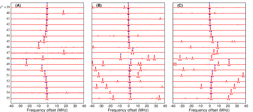
Figure 1: Loomis-Wood plots for $J^{\prime\prime}=39$ to $J^{\prime\prime}=55$ ${}^{a}R_{0,1}$ series of excited vibrational state transitions of thioformamide: (A) $K_{a}=5$, $K_{c}=J^{\prime\prime}-K_{a}$ of $\nu_{12}=1$ state, (B) $K_{a}=0$ of $\nu_{9}=1$ state, and (C) $K_{a}=1$, $K_{c}=J^{\prime\prime}-K_{a}+1$ of $\nu_{9}=1$ state. Blue stars indicate the lines that were effectively assigned to each series. For series (A) and (C), the $J^{\prime\prime}=47$ and $J^{\prime\prime}=48$ transitions are out of the plot range by $\pm 40$ MHz.

2.2 Spectroscopy

The measurements in the frequency range under investigation were performed using the Lille spectrometer (Zakharenko et al., 2015), equipped with a fast-scan mode (Motiyenko et al., 2019). The frequency ranges 150$-$330 and 400$-$660 GHz were covered with various active and passive frequency multipliers from VDI Inc., and an Agilent synthesizer (12.5$-$18.25 GHz) was used as the reference radiation source. The absorption cell was a stainless-steel tube (6 cm diameter, 220 cm long). During measurements, the sample was kept at a pressure of about 10 Pa and at room temperature, the line width was determined mostly by Doppler broadening. Estimated uncertainties for measured line frequencies are 30 kHz, 50 kHz, 100 kHz, and 200 kHz depending on the observed signal-to-noise ratio (S/N) and the frequency range.

3 Spectroscopic analysis

3.1 Ground states of parent, ³⁴S, ¹³C, and ¹⁵N isotopic species

Thioformamide is a prolate asymmetric top close to the symmetric top limit ($\kappa\approx 0.98$). Structural parameters obtained from an experimental study (Sugisaki et al., 1974) and theoretical calculations (Kowal, 2006) suggest that the molecule is planar. As was determined by Sugisaki et al. (1974), thioformamide has a strong $a$-component of the dipole moment, $\mu_{a}=3.99(2)$ D, and a weak $b$-component $\mu_{b}=0.13(25)$ D.

For the initial assignment of the rotational spectrum of thioformamide, we used spectral predictions calculated using a set of rigid rotor and quartic centrifugal distortion constants. The rigid rotor constants were taken from the previous study (Sugisaki et al., 1974). The quartic centrifugal distortion constants were obtained from the theoretical calculations of harmonic force field preceded by molecular geometry optimization. The theoretical calculations were performed using the density functional theory (DFT) employing Becke’s three-parameter hybrid functional (Becke, 1988), and the Lee, Yang, and Parr correlation functional (B3LYP) (Lee et al., 1988). The 6-311++G(3df, 2pd) wave function was employed in the B3LYP calculations.

On the basis of the calculated predictions, the assignment of the ground-state transitions of the parent isotopic species of thioformamide was straightforward as the frequencies of transitions with low $K_{a}$ values were predicted within a few MHz. Several refinements of the Hamiltonian parameter data set were needed to accurately fit and predict the transitions with higher $K_{a}$ values. In addition to the parent isotopolog, we were able to assign the lines of the ³⁴S, ¹³C, and ¹⁵N isotopic species of thioformamide in natural abundance, which is correspondingly 4.25%, 1.1%, and 0.4%. As for the ground state of the parent species, the initial assignment of isotopologs was based on spectral predictions obtained from a set of rigid rotor constants determined by Sugisaki et al. (1974) and centrifugal distortion constants of the parent species determined in this study. We note that the assignment of the isotopic species was greatly facilitated by the results of Sugisaki et al. (1974). Owing to strong spectral congestion of weak lines caused in particular by sample impurities, it would be practically impossible to distinguish characteristic spectral patterns of isotopologs. Therefore the assignment was only possible by direct comparison of the experimental spectra with calculated predictions.

All the assigned transitions were fit to a Watson $A$-reduction Hamiltonian in $I^{r}$ coordinate representation. In addition, we also tested $S$-reduction Hamiltonian, as the asymmetry parameter of thioformamide is quite close to the symmetric top limit. We applied both reductions in the least-squares fit of the assigned ground-state transitions of the parent isotopolog, and obtained the fits of similar quality in terms of root-mean-square and weighted root-mean-square deviations, and number of lines that were fit. However, in the case of the $S$-reduction Hamiltonian, the least-squares fit required one more parameter than the $A$-reduction. This allowed us to suggest that for thioformamide, $A$-reduction Hamiltonian may be preferred to $S$-reduction. The complete list of measured rotational transitions in the ground state of parent isotopic species of thioformamide is presented in Table 6 available at the CDS. Owing to its significant size, we show only a part of Table 6 as an example here.

The results of the fits including $S$- and $A$-reduction tests are given in Table 1. All the data sets were fit within experimental accuracy. For each isotopic species we determined the full set of fourth order centrifugal distortion constants, as well as several sixth- and eighth-order (in the case of the parent and ³⁴S species) constants. For the ground state of the parent isotopic species, we were able to assign about 30 weak $b$-type transitions. To correctly reproduce the intensities of the $b$-type transitions with respect to other assigned neighboring lines, we found that the $\mu_{b}$ value should be scaled to about 0.2 D, which is higher by a factor of 1.5 than the $\mu_{b}$ value determined by Sugisaki et al. (1974). We are not able to provide a more accurate determination of the $\mu_{b}$ value and its uncertainty because we were unable to perform a comparison with the intensities of $a$-type transitions of the ground state of parent isotopic species here. The assigned $a$- and $b$-type transitions are significantly spaced on the frequency scale, whereas baseline and radiation source intensity variations make this comparison very inaccurate. Moreover, we were unable to resolve the nuclear quadrupole hyperfine structure owing to the ^14N atom in the Doppler-limited spectra of thioformamide.

Table 1: Ground-state rotational constants of parent, ³⁴S, ¹³C, and ¹⁵N isotopic species of thioformamide

S-reduction		A-reduction
Parameters	Parent	Parameters	Parent	H2NCH^34S	H2N^13CHS	H_2^15NCHS
$A$ (MHz)	61754.8040(80)	$A$ (MHz)	61754.8024(81)	61632.104(56)	60002.038(75)	61319.746(96)
$B$ (MHz)	6101.76611(14)	$B$ (MHz)	6101.80024(14)	5952.38931(27)	6085.09318(38)	5919.64877(56)
$C$ (MHz)	5549.86284(13)	$C$ (MHz)	5549.82889(13)	5424.98705(26)	5521.38188(34)	5395.37815(56)
$D_{J}$ (kHz)	2.559762(22)	$\Delta_{J}$ (kHz)	2.601528(25)	2.483353(41)	2.561801(64)	2.470969(87)
$D_{JK}$ (kHz)	-48.89300(51)	$\Delta_{JK}$ (kHz)	-49.14361(51)	-48.1177(11)	-47.6244(13)	-48.9717(24)
$D_{K}$ (kHz)	1508.12(41)	$\Delta_{K}$ (kHz)	1508.26(42)	1522.0(31)	1490.7(37)	1513.4(57)
$d_{1}$ (kHz)	-0.379115(39)	$\delta_{J}$ (kHz)	0.379174(36)	0.354556(60)	0.384478(83)	0.35373(14)
$d_{2}$ (kHz)	-0.020822(17)	$\delta_{K}$ (kHz)	16.9294(35)	16.362(10)	16.757(13)	15.975(21)
$H_{J}$ (Hz)	0.0018292(39)	$\Phi_{J}$ (Hz)	0.0019788(40)	0.0018384(61)	0.001885(10)	0.001848(13)
$H_{JK}$ (Hz)	-0.02017(19)	$\Phi_{JK}$ (Hz)	-0.02012(19)	-0.01759(10)	-0.01902(22)	-0.01806(41)
$H_{KJ}$ (Hz)	-5.4240(16)	$\Phi_{KJ}$ (Hz)	-5.4267(16)	-5.3629(82)	-5.2389(47)	-5.241(13)
$H_{K}$ (Hz)	144.5(62)	$\Phi_{K}$ (Hz)	143.4(63)	0.0	0.0	0.0
$h_{1}$ (Hz)	0.0006741(67)	$\phi_{J}$ (Hz)	0.0006843(61)	0.0006279(98)	0.000687(14)	0.000643(24)
$h_{2}$ (Hz)	0.0000590(45)	$L_{JK}$ (mHz)	-0.01139(23)	0.0	0.0	0.0
$L_{JK}$ (mHz)	-0.01315(23)	$L_{KKJ}$ (mHz)	0.5306(15)	0.499(16)	0.0	0.0
$L_{KKJ}$ (mHz)	0.5352(15)
N	1066		1066	773	716	261
$J_{\mathrm{max}}$, $K_{a,\mathrm{max}}$	59, 27		59, 27	59, 19	59, 17	58, 15
$\sigma$ (MHz)	0.028		0.028	0.028	0.039	0.44
$\sigma_{w}$	0.57		0.57	0.56	0.76	0.86

3.2 Excited vibrational states $\varv_{12}=1$, and $\varv_{9}=1$ of the parent isotopic species

For the parent isotopic species, the rotational transitions of the lowest excited vibrational states formed quite easily distinguishable patterns of satellite lines in the observed spectrum. The two lowest vibrational modes of thioformamide are NH2 out-of-plane wagging $\nu_{12}$, and in-plane bending of NCS moiety $\nu_{9}$. The vibrational frequencies of these modes are 393 and 457 cm^-1, respectively, as determined from the analysis of relative intensities by Sugisaki et al. (1974). The analysis of the excited states started with the assignment of $K_{a}=0$ series of lines of $\varv_{12}=1$ state and continued to higher $K_{a}$ values. The series of $K_{a}=6$ lines was found to be perturbed as some of the lines exhibited quite large and irregular deviations from predicted frequencies. For the $\varv_{9}=1$ we found that even $K_{a}=0$ and $K_{a}=1$ series of lines were perturbed in a similar way.

The perturbations are illustrated on Fig. 1, where Loomis-Wood type diagrams are shown for the ${}^{a}R_{0,1}$ series of transitions with $J^{\prime\prime}$ in the range from 39 to 55, and where $J^{\prime\prime}$ is the upper level quantum number. Each diagram is represented by a superposition of experimental spectra centered on the corresponding series transition frequency. The transition frequencies were calculated on the basis of the results of a single-state fit that does not take any vibrational state coupling into account. The analysis of Fig. 1 shows that the lines of series (A) and (C) that represent $K_{a}=5$, $K_{c}=J^{\prime\prime}-K_{a}$ transitions of $\varv_{12}=1$ state and $K_{c}=J^{\prime\prime}-K_{a}+1$ of $\varv_{9}=1$ state, respectively, significantly deviate from calculated values for $J^{\prime\prime}$ in the range 45 to 51. For the two series, the deviations from calculated frequencies are approximately the same, but with opposite sign. In addition, relatively smaller deviations are observed for $J^{\prime\prime}=47$ to 49 of series (B), which represents $K_{a}=0$ transitions of the $\varv_{9}=1$ state. This behavior is a typical example of local resonances coupling $\varv_{12}=1$ and $v_{9}=1$ states. In this case, the coupling Hamiltonian may be presented in the following block-diagonal form:

$$H=\left(\begin{array}[]{cc}H_{\mathrm{rot}}^{(12)}&H_{\mathrm{c}}\\ H_{\mathrm{c}}&H_{\mathrm{rot}}^{(9)}+\Delta E\\ \end{array}\right),$$ (1)

where $H_{\mathrm{rot}}^{(12)}$ and $H_{\mathrm{rot}}^{(9)}$ are the standard rotational Watson $A$-reduction Hamiltonians, $\Delta E$ is the energy difference between two coupled states, and $H_{\mathrm{c}}$ is the off-diagonal interaction term.

When molecular planarity is assumed, the equilibrium configuration of thioformamide is described by the $C_{s}$ point group. The vibrational modes $\nu_{12}$ and $\nu_{9}$ belong to $A^{\prime\prime}$ and $A^{\prime}$ irreducible representations of the group, respectively. As a result, Coriolis interaction between the two modes is allowed along the $a$ and $b$ axes, and the Hamiltonian $H_{\mathrm{c}}$ we used is expressed as

$$\begin{array}[]{l}H_{\mathrm{c}}=i(G_{a}+G_{a}^{J}P^{2}+G_{a}^{K}P_{z}^{2}+...)P_{z}+\\ i(G_{b}+G_{b}^{J}P^{2}+G_{b}^{K}P_{z}^{2}+G_{b}^{JK}P^{2}P_{z}^{2}...)P_{x}\end{array},$$ (2)

where $G_{a}$ and $G_{b}$ are the Coriolis coupling constants, and all other parameters are their respective centrifugal distortion corrections.

In search of an initial global solution of the two-state coupling problem using the Hamiltonian in Eq. 1, we used a method that was previously successfully applied for a similar case (Motiyenko et al., 2018). Because the $\Delta E$, and $G_{a}$ and $G_{b}$ parameters are usually highly correlated, and given the absence of sufficiently accurate initial values of these parameters, we fixed $\Delta E$ to a series of reasonable values. The range of $\Delta E$ values was estimated from the energy difference between $\varv_{12}=1$ and $\varv_{9}=1$ states determined by Sugisaki et al. (1974). Taking the uncertainties of the vibrational frequencies of the $\nu_{12}$ and $\nu_{9}$ modes into account, we generated a set of $\Delta E$ values that varied from 35 cm^-1 to 114 cm^-1 with a step of about 0.03 cm^-1. For each fixed $\Delta E$ from the set we performed a least-squares fit using the Hamiltonian in Eq. 1 in which $G_{a}$ and $G_{b}$ were varied. A global solution corresponding to the minimum root-mean-square deviation of the fit was found for $\Delta E\approx$ 60 cm^-1. Then, $\Delta E$ was allowed to vary in the fit along with $G_{a}$ and $G_{b}$ starting from its approximate value found at the previous step. In this manner, we were able to fit the perturbed transitions shown in Fig. 1 within experimental accuracy and to accurately predict the most perturbed transitions that were out of the range of the Loomis-Wood plot. The following assignment process was straightforward and similar to the assignment of the ground state with several cycles of refinement of the Hamiltonian parameters. The results of the global fit are presented in Table 2. In terms of signs and orders of magnitude, the determined centrifugal distortion constants of the two excited vibrational states agree with the corresponding ground state parameters. The final value of energy difference between $\varv_{12}=1$ and $\varv_{9}=1$ states, 59.991696(57) cm^-1, also agrees with the energy difference of about 64 cm^-1 from the analysis of relative intensities by Sugisaki et al. (1974).

Table 2: Rotational constants of $\varv_{12}=1$, and $\varv_{9}=1$ excited vibrational states of the parent isotopolog of thioformamide.

Parameters	$\varv_{12}=1$	$\varv_{9}=1$
$A$ (MHz)	61118.626(83)	61890.776(81)
$B$ (MHz)	6098.12788(52)	6101.04527(57)
$C$ (MHz)	5552.46610(25)	5544.50067(27)
$\Delta_{J}$ (kHz)	2.608050(46)	2.582672(44)
$\Delta_{JK}$ (kHz)	-48.371(17)	-47.945(17)
$\Delta_{K}$ (kHz)	1433.5(12)	1561.6(16)
$\delta_{J}$ (kHz)	0.377740(70)	0.377563(72)
$\delta_{K}$ (kHz)	16.3958(97)	18.7564(88)
$\Phi_{J}$ (Hz)	0.0019722(68)	0.0019123(65)
$\Phi_{JK}$ (Hz)	-0.02115(16)	-0.01684(19)
$\Phi_{KJ}$ (Hz)	-4.9201(99)	-5.961(12)
$\phi_{J}$ (Hz)	0.000670(14)	0.000648(13)
$L_{KKJ}$ (mHz)	0.423(19)	0.450(25)
$\Delta E$ (MHz) / (cm-1)	1798505.8(17) / 59.991696(57)
$G_{a}$ (MHz)	25010.4(24)
$G_{a}^{J}$ (MHz)	0.00665(59)
$G_{b}$ (MHz)	-829.39(51)
$G_{b}^{J}$ (MHz)	0.003478(42)
N	690	686
$\sigma$ (MHz)	0.028	0.027
$\sigma_{w}$	0.68	0.64

3.3 Rotational spectrum predictions

On the basis of the parameter set presented in Table 1, we calculated spectrum predictions of the ground-state rotational transitions of the parent isotopic species of thioformamide. The predictions calculated at $T=300$ K are given in Table 7. Owing to its significant size, the complete version of Table 7 is presented at the Centre de Données at Strasbourg (CDS). Here only a part of the table is presented for illustration purposes. The table includes quantum numbers, calculated transition frequencies and corresponding uncertainties, the base 10 logarithm of the integrated transition intensity in the units of JPL and CDMS catalogs, nm²MHz, and the lower state energy in cm^-1. Rotational $Q_{rot}$ and vibrational $Q_{v}$ partition functions used for the calculation of spectral predictions are given in Table 8. The total partition function is thus $Q_{tot}=Q_{rot}\times Q_{v}$. The vibrational contribution to the partition function is calculated as ${\displaystyle Q_{v}=\prod_{i}\left(1-e^{-E_{i}/k_{B}T}\right)^{-1}}$, see equation 3.60 from Gordy & Cook (1984), where $E_{i}$ is the energy of $i$-th vibrational mode. The $E_{i}$ values for the $\nu_{12}$ and $\nu_{9}$ modes were taken from the relative intensity measurements by Sugisaki et al. (1974), and for all other vibrational modes from the theoretical calculations using the vibrational self-consistent field method and taking second-order perturbative energy correction into account (Kowal, 2006).

The nuclear quadrupole hyperfine structure was not taken into account in spectral predictions. In the previous study (Sugisaki et al., 1974), a limited number of resolved hyperfine transitions did not allow an accurate determination of nuclear quadrupole coupling parameters because two different but relatively close sets of such parameters were obtained. Therefore the nuclear quadrupole hyperfine structure in the rotational spectrum of thioformamide may be a topic of future studies. We also verified that the hyperfine structure may be ignored for the rotational lines used for the search of thioformamide in the ISM when the spectral resolution of the ReMoCA survey is taken into account. For this purpose, we calculated two sets of spectral predictions of the ground-state rotational transitions of thioformamide using the two sets of nuclear hyperfine parameters from Sugisaki et al. (1974). In the two sets of predictions, the strongest $a$-type rotational transitions exhibit relatively small hyperfine splittings below the spectral resolution of the ReMoCA survey.

4 Search for thioformamide toward Sgr B2(N)

4.1 Observations

We used data acquired with the imaging spectral line survey ReMoCA performed with ALMA toward Sgr B2(N). The observational setup and data reduction of the ReMoCA survey were described in Belloche et al. (2019). In short, the frequency range from 84.1 GHz to 114.4 GHz was fully covered with a spectral resolution of 488 kHz (1.7 to 1.3 km s^-1). The interferometric observations achieved an angular resolution (half-power beam width, HPBW) varying between $\sim$0.3$\arcsec$ and $\sim$0.8$\arcsec$, with a median value of 0.6$\arcsec$. This corresponds to $\sim$4900 au at the distance of Sgr B2 (8.2 kpc, Reid et al., 2019). The rms sensitivity ranged between 0.35 mJy beam^-1 and 1.1 mJy beam^-1, with a median value of 0.8 mJy beam^-1. The phase center was set to ($\alpha,\delta$)_J2000= ($17^{\rm h}47^{\rm m}19{\aas@@fstack{s}}87,-28^{\circ}22^{\prime}16{\aas@@fstack{\prime\prime}}0$), a position that is halfway between the two main hot molecular cores Sgr B2(N1) and Sgr B2(N2) that are separated by 4.9$\arcsec$ or $\sim$0.2 pc in projection onto the plane of the sky.

Here we analyze the spectra toward Sgr B2(N2) at ($\alpha,\delta$)_J2000= ($17^{\rm h}47^{\rm m}19{\aas@@fstack{s}}860$, $-28^{\circ}22\arcmin 13{\aas@@fstack{\prime\prime}}40$) and toward the offset position Sgr B2(N1S) defined by Belloche et al. (2019). This offset position is located at ($\alpha,\delta$)_J2000= ($17^{\rm h}47^{\rm m}19{\aas@@fstack{s}}870$, $-28^{\circ}22\arcmin 19{\aas@@fstack{\prime\prime}}48$), about 1$\arcsec$ to the south of Sgr B2(N1). It was chosen for two reasons: the velocity dispersion (full width at half maximum, FWHM) of its molecular emission lines is small ($\sim$5 km s^-1), thus reducing the spectral confusion, and its continuum emission has a lower optical depth than the partially optically thick emission toward the peak position of the main hot core Sgr B2(N1), thus allowing us to peer deeper into the molecular line emission region. Compared to Belloche et al. (2019), we used a new version of our data set for which we have improved the separation of the continuum and line emission (see Melosso et al., 2020).

We modeled the spectra of Sgr B2(N1S) and Sgr B2(N2) with the software Weeds (Maret et al., 2011) under the assumption of local thermodynamic equilibrium (LTE), which is appropriate given the high densities that characterize the regions where hot-core emission is detected in Sgr B2(N) ($>1\times 10^{7}$ cm^-3, see Bonfand et al., 2019). We derived a best-fit synthetic spectrum of each molecule separately, and then added the contributions of all identified molecules together. Each species was modeled with a set of five parameters: size of the emitting region ($\theta_{\rm s}$), column density ($N$), temperature ($T_{\rm rot}$), line width ($\Delta V$), and velocity offset ($V_{\rm off}$) with respect to the assumed systemic velocity of the source, $V_{\rm sys}=62$ km s^-1 for Sgr B2(N1S) and $V_{\rm sys}=74$ km s^-1 for Sgr B2(N2).

Table 3: Parameters of our best-fit LTE model of selected complex organic molecules toward Sgr B2(N1S), and upper limit for thioformamide.

Molecule	Status	$N_{\rm det}$	$\theta_{\rm s}$	$T_{\mathrm{rot}}$	$N$	$F_{\rm vib}$	$\Delta V$	$V_{\mathrm{off}}$	$\frac{N_{\rm ref}}{N}$
			(′′)	(K)	(cm-2)		(km s-1)	(km s-1)
CH3OH, $\varv=0$⋆	d	35	2.0	230	2.0 (19)	1.00	5.0	$0.2$	1
$\varv_{\rm t}=1$	d	17	2.0	230	2.0 (19)	1.00	5.0	$0.2$	1
$\varv_{\rm t}=2$	d	4	2.0	230	2.0 (19)	1.00	5.0	$0.2$	1
$\varv_{\rm t}=3$	t	1	2.0	230	2.0 (19)	1.00	5.0	$0.2$	1
13CH3OH, $\varv=0$	d	10	2.0	230	1.2 (18)	1.00	5.0	$0.2$	17
$\varv_{\rm t}=1$	d	6	2.0	230	1.2 (18)	1.00	5.0	$0.2$	17
CH318OH, $\varv=0$	t	1	2.0	230	2.0 (17)	1.00	5.0	$0.2$	100
$\varv_{\rm t}=1$	n	0	2.0	230	2.0 (17)	1.00	5.0	$0.2$	100
CH3SH, $\varv=0$	d	6	2.0	250	5.5 (17)	1.00	5.0	$0.0$	36
$\varv_{\rm t}=1$	t	0	2.0	250	5.5 (17)	1.00	5.0	$0.0$	36
$\varv_{\rm t}=2$	n	0	2.0	250	5.5 (17)	1.00	5.0	$0.0$	36
NH2CHO⋆	d	34	2.0	160	2.9 (18)	1.09	6.0	$0.0$	1
NH2CHS, $\varv=0$	n	0	2.0	160	$<$ 4.2 (15)	1.05	6.0	$0.0$	$>$ 701

Table 4: Parameters of our best-fit LTE model of selected complex organic molecules toward Sgr B2(N2) and upper limit for thioformamide.

Molecule	Status	$N_{\rm det}$	$\theta_{\rm s}$	$T_{\mathrm{rot}}$	$N$	$F_{\rm vib}$	$\Delta V$	$V_{\mathrm{off}}$	$\frac{N_{\rm ref}}{N}$
			(′′)	(K)	(cm-2)		(km s-1)	(km s-1)
CH3OH⋆	d	60	1.4	160	4.0 (19)	1.00	5.4	$-0.2$	1
CH3SH	d	13	1.4	180	3.4 (17)	1.00	5.4	$-0.5$	118
NH2CHO⋆	d	43	0.8	200	2.6 (18)	1.17	5.5	$0.2$	1
NH2CHS, $\varv=0$	n	0	0.8	200	$<$ 2.8 (15)	1.12	5.5	$0.2$	$>$ 919

Table 5: Rotational temperatures derived from population diagrams toward Sgr B2(N1S).

Molecule	States	$T_{\rm fit}$
		(K)
CH3OH	$\varv=0$, $\varv_{\rm t}=1$, $\varv_{\rm t}=2$, $\varv_{\rm t}=3$	234.9 (7.7)
13CH3OH	$\varv=0$, $\varv_{\rm t}=1$	232 (21)
CH318OH	$\varv=0$, $\varv_{\rm t}=1$	195 (52)
CH3SH	$\varv=0$, $\varv_{\rm t}=1$	335 (90)

4.2 Nondetection of thioformamide

We searched for rotational emission of thioformamide toward Sgr B2(N1S) and Sgr B2(N2) by comparing the ReMoCA spectra to LTE synthetic spectra of thioformamide obtained with the parameters derived for formamide, NH₂CHO, by Belloche et al. (2019) and Belloche et al. (2017), respectively, keeping only the column density of thioformamide as a free parameter. We found no evidence for emission of thioformamide toward either source. Figures 2 and 3 illustrate the nondetection toward Sgr B2(N1S) and Sgr B2(N2), respectively, and the upper limits to the column density of thioformamide are indicated in Tables 3 and 4, respectively, along with the parameters previously obtained for formamide.

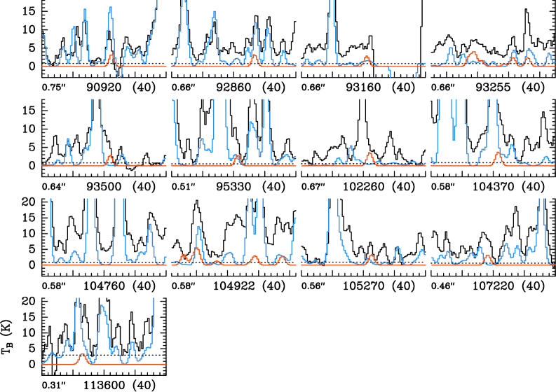
Figure 2: Transitions of NH₂CHS, $\varv=0$ covered by our ALMA survey. The synthetic spectrum of NH₂CHS, $\varv=0$ we used to derive the upper limit to its column density is displayed in red and overlaid on the observed spectrum of Sgr B2(N1S) shown in black. The blue synthetic spectrum contains the contributions from all molecules identified in our survey so far, but not from the species shown in red. The central frequency and width are indicated in MHz below each panel. The angular resolution (HPBW) is also indicated. The $y$-axis is labeled in brightness temperature units (K). The dotted line indicates the $3\sigma$ noise level.

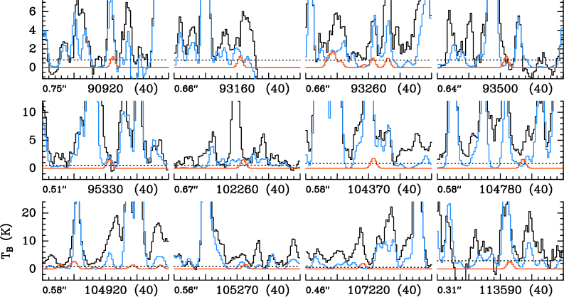
Figure 3: Same as Fig. 2, but for Sgr B2(N2).

4.3 Comparison to other molecules

In order to place the nondetection of thioformamide into an astrochemical context, we wished to compare the upper limits on its column density to the column densities of other complex organic molecules. In addition to formamide, we chose methanol, CH₃OH, and methanethiol, CH₃SH, which were both detected toward both hot cores (Belloche et al., 2013; Müller et al., 2016). Table 4 lists the parameters obtained for methanol and methanethiol by Müller et al. (2016) toward Sgr B2(N2) on the basis of the EMoCA survey, which was also performed with ALMA (Belloche et al., 2016).

We derived the column densities of methanol and methanethiol toward Sgr B2(N1S) using the ReMoCA survey. In order to obtain the LTE parameters of methanol, we also modeled the emission of its isotopologs, ¹³CH₃OH and CH${}_{3}^{18}$OH. We used the spectroscopic entries available in the CDMS database to compute the synthetic spectra: version 3 of entry 32504 for CH₃OH, version 2 of entry 33502 for ¹³CH₃OH, version 1 of entry 34504 for CH${}_{3}^{18}$OH, and version 2 of entry 48510 for CH₃SH.

Our best-fit synthetic spectra are shown in Figs. 6-13 for methanol and its isotopologs, and in Figs. 14 and 15 for methanethiol. The parameters of these LTE models are listed in Table 3. Methanol is detected in its vibrational ground state and in its first two vibrational states (Figs. 6–8). It is only tentatively detected in the third vibrational state (Fig. 9). ¹³CH₃OH is detected in both the ground and first vibrational states (Figs 10 and 11). There are hints of emission from CH${}_{3}^{18}$OH (Figs. 12 and 13), but because only one transition is not much contaminated by emission from other species, the identification of this isotopolog and the derived column density are uncertain. The true column density might well be lower. For certain CH3OH lines, the actually observed ReMoCA spectrum shows much weaker emission than predicted by the LTE model or even absorption. This is due to absorption from the extended envelope of Sgr B2(N) and/or due to peculiarities in the excitation of methanol that lead to non-LTE effects. These may result in inversion for some lines and in anti-inversion (“overcooling”) for others; for a discussion, see Section 5.4 of Belloche et al. (2013).

Methanethiol is clearly detected in its vibrational ground state (Fig. 14). Three transitions from within $\varv_{\rm t}=1$ match the observed lines well (Fig. 15), but they account for only $\sim$50% of the detected signal, the rest being emitted by other species included in our full model. This is not sufficient to claim a firm detection of this state, but we consider it as tentatively detected. Emission from several transitions of $\varv_{\rm t}=2$ significantly contributes to the detected signal (Fig. 16), but no line can be firmly identified, and so no detection of this state can be claimed. However, we include it in our full model of the Sgr B(N1S) spectrum.

We used the lines that are not too strongly contaminated to produce population diagrams for methanol, its isotopologs, and methanethiol. These diagrams are shown in Figs. 17–20. The rotational temperatures formally derived from fits to these population diagrams are reported in Table 5. We adopted a temperature of 230 K to model the emission of methanol and its isotopologs. The temperature of methanethiol is not well constrained, and we set it to 250 K, which gives a reasonable fit to the emission of its ground and first vibrational states.

The LTE synthetic spectra of Sgr B2(N1S) were computed assuming a diameter (FWHM) of 2$\arcsec$ for the emission of methanol and methanethiol, as was done for formamide and other species reported by Belloche et al. (2019) toward Sgr B2(N1S). This size is approximately three times larger than the angular resolution of the ReMoCA survey, and thus its exact value does not affect the derivation of the column density significantly. A two-dimensional Gaussian fit to the integrated intensity maps of the least contaminated transitions of methanethiol yields a mean size of $\sim$2.2$\arcsec$ with an rms dispersion of $\sim$0.3$\arcsec$, consistent with our size assumption. The emission of higher-energy transitions of CH₃OH and ¹³CH₃OH also has a typical size of about 2$\arcsec$, while lower-energy transitions show more extended emission up to $\sim$5$\arcsec$ (Fig. 4). This indicates that in addition to the compact hot-core component, there is also more extended emission of methanol in the envelope of the main hot core. This probably explains why the most optically thick transitions are not well reproduced by our synthetic model: their peak intensities are overestimated (see Fig. 6). Our model does not account for extended methanol emission at lower densities in the envelope, which likely acts as an opaque screen at the frequencies of optically thick transitions, thus attenuating their peak intensities.

Figure 4: Deconvolved emission size of uncontaminated methanol transitions as a function of upper-level energy. Panels a and b show the major and minor axes (FWHM), respectively.

5 Discussion

No emission of thioformamide was detected in the ReMoCA spectra of Sgr B2(N1S) and Sgr B2(N2). The column density upper limits derived from our LTE analysis indicate that thioformamide is at least $\sim$700 and $\sim$900 times less abundant than formamide in Sgr B2(N1S) and Sgr B2(N2), respectively. This is at first sight surprising when we compare it to methanethiol, which is only $\sim$40 and 120 times less abundant than methanol in these sources, respectively. We examine below which chemical processes might be responsible for this large difference.

Astrochemical kinetic modeling of sulfur-bearing species has mostly been limited to molecules only as large as H₂CS (e.g., Charnley, 1997), but Müller et al. (2016) constructed a chemical network for methanethiol and ethanethiol that was based mostly on grain-surface chemistry (while also including the necessary gas-phase destruction mechanisms). To our knowledge, no networks exist for the production of interstellar thioformamide. It is therefore not possible to compare the observational results directly with a chemical model. However, guided by the modeling results for related molecules, we may draw qualified conclusions as to the origin of the different behavior of formamide/thioformamide versus methanol/methanethiol.

Recently, Jin & Garrod (2020) presented rate equation-based chemical kinetic models that included a range of new, nondiffusive reaction mechanisms on cold dust-grain surfaces. In the usual scenario, the chemistry at low temperatures is dominated by mobile H atoms, which diffuse on the grain or ice surface until they meet and react with some relatively immobile species; this might be, for example, a heavier atom adsorbed from the gas such as O, a molecule such as CO, or a radical produced by a previous surface reaction. The inclusion of nondiffusive processes in the models occasionally allows surface radicals to react with each other without significant diffusion being required (which is largely prohibited at low temperatures). When produced on grain surfaces through any chemical reaction, radicals may sometimes be formed in close proximity to each other, either in direct contact or within a short distance, such that they may occasionally react as soon as either one is formed in the presence of the other. The exothermicity of the initiating reaction would also allow some degree of surface diffusion to take place, allowing nearby but noncontiguous species to meet after the initiating reaction. Jin & Garrod (2020) referred to this overall nondiffusive process as the three-body (3-B) reaction mechanism. (Other nondiffusive mechanisms also exist that are initiated by other processes). This 3-B mechanism has been explored experimentally over the past several years and appears to be effective in producing complex organic molecules, especially those derived from the hydrogenation of CO (e.g., Fedoseev et al., 2017). This general mechanism is usually present automatically in microscopic kinetic Monte Carlo models of grain-surface chemistry, which consider the explicit positions of surface species, but must be explicitly coded into models that are based on rate equations.

Garrod et al. (2020) applied the nondiffusive processes investigated by Jin & Garrod (2020) to hot-core chemical models; as in previous work, the physical evolution involves a cold-collapse stage during which the dust temperature falls from (in this model) approximately 15 K down to 8 K as the visual extinction rises. The collapse stage is followed by a time-dependent warm-up of the gas and dust, from 8 to 400 K. In their “final” model, encompassing all of the new mechanisms and updates, Garrod et al. (2020) find that formamide is produced almost entirely during the cold stage, as the result of both diffusive and nondiffusive reaction processes on the dust or ice surfaces, with those molecules then becoming embedded in the ice mantles and returning to the gas phase when high temperatures ($>$100 K) are reached. The critical nondiffusive step in this formation process is the reaction between HCO and NH, to produce HNCHO, which may be further hydrogenated by diffusive H-addition to produce NH₂CHO. The radicals HCO and NH may be formed by the diffusive addition of H to CO and N, respectively, which may on occasion react spontaneously when formed nearby (i.e., the 3-B reaction).

Figure 5 shows results from the Garrod et al. (2020) model for a selection of species related to thioformamide and methanethiol for the cold collapse phase (during which most solid-phase formamide is produced). The collapse from a density of $3\times 10^{3}$ to $2\times 10^{8}$ cm^-3 takes approximately $9.4\times 10^{5}$ yr. Methanethiol is explicitly included in the chemical model, using the sulfur network presented by Müller et al. (2016), with the same sulfur elemental abundance of $8\times 10^{-8}n_{\mathrm{H}}$.

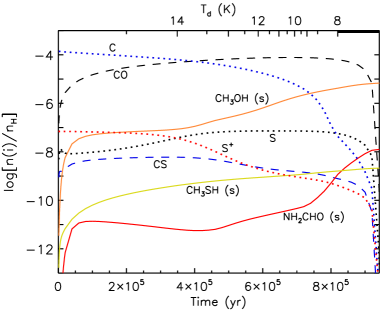
Figure 5: Fractional abundances with respect to total hydrogen for selected gas- and solid-phase species during the cold-collapse stage of hot core evolution based on data from the “final” model of Garrod et al. (2020). Solid-phase species are marked “(s)” and are plotted with a solid line. The dust temperature is indicated on the top axis and has a lower limit of 8 K.

The fractional abundance of solid-phase (marked “(s)”) methanethiol gradually grows during the collapse, reaching a final abundance of a few $10^{-9}$. An abundance of this order is reached at around $7\times 10^{5}$ yr. As with methanol forming from grain surface CO, methanethiol is formed by repeated H addition to CS. The CS is accreted from the gas phase, forming mainly as the result of reactions of S⁺ with CH (whose abundance tracks with that of gas-phase atomic C), leading to CS⁺. Reaction with H₂ to give HCS⁺, followed by recombination with electrons completes the conversion into CS.

Solid-phase formamide abundance is also shown in Fig. 5; it should be noted that the above-described 3-B process for formamide only leads to substantial formation of this molecule at late times in the model, when temperatures are very low ($<\sim$9 K) and densities high. The slower surface diffusion of atomic H and its reduced adsorption from the gas phase under these conditions allow the radicals to build up a somewhat greater surface coverage, which increases the influence of the 3-B process.

In a similar way to formamide, thioformamide might also be expected to form at low temperatures or late times through the 3-B process through the reaction HCS + NH $\rightarrow$ HNCHS, followed by diffusive hydrogen addition to give NH₂CHS. However, in this case, the necessary gas-phase precursor species, CS, is much lower in abundance at late times when formamide or thioformamide production should be highest. Gas-phase CS abundance begins to fall relative to CO, starting at around $4\times 10^{5}$ yr, as the result of the switch-over from S⁺ to neutral S as the dominant sulfur carrier in the gas phase. The drop in S⁺ together with the gradual fall in atomic C and CH abundances ultimately reduces the CS abundance, meaning that toward the end time in the model, production of NH₂CHS would be much weaker (relative to NH₂CHO) than if the earlier gas-phase CS abundance had been preserved. The gas-phase ratio of CS/CO at a time $4\times 10^{5}$ yr is approximately $1.1\times 10^{-4}$, while at a time of $9\times 10^{5}$ yr, when NH₂CHO production is at its peak, this ratio is about $9.2\times 10^{-6}$, which is a decrease of about 12 times. At yet later times, the ratio continues to fall.

We therefore suggest that this fall in gas-phase CS at just the period when surface production of NH₂CHS should be most efficient is the underlying cause for the weaker production of NH₂CHS as compared with the production of CH₃SH. The latter can form more consistently at earlier times and over a broader range of temperatures because it is produced through direct H-addition and is independent of the more restrictive 3-B process.

As a point of comparison, we note that the solid-phase CH₃SH abundance presented in Fig. 5 is similar to that found by Müller et al. (2016) because it is formed by the same standard process of diffusive H-addition. We also note that the reduced elemental sulfur abundance that is used in both models, while typical for such studies, could produce a different result from a model using the much higher solar or diffuse-cloud S abundances. However, the ratio of methanethiol to methanol in the model is about two orders of magnitude lower than the observational value, therefore a higher elemental sulfur abundance in the models might be justified on this basis. The dominant form of this sulfur in dense interstellar regions is still uncertain and might affect the chemistry described above.

It is possible that some of the species discussed here may be formed during the warm-up stage, likely through radical-radical reactions driven by cosmic-ray-induced UV photodissociation. Based on the Garrod et al. (2020) models, we do not expect this to make a substantial contribution to the relative abundances of methanol and formamide and the corresponding sulfur derivatives. It has also been suggested that gas-phase mechanisms might play a role in the production of formamide in hot cores (e.g., Barone et al., 2015) through the reaction NH₂ + H₂CO $\rightarrow$ NH₂CHO + H. However, again, the models of Garrod et al. (2020) suggest that the effect of such processes, even using the rates provided by Skouteris et al. (2017), is slight compared to grain-surface production. It is unknown whether a similar process might contribute substantially to the production of thioformamide in the gas phase.

A more robust investigation of the possible production of interstellar thioformamide would of course involve the use of a dedicated chemical network for that and related species; we hope to carry out such a study in the future.

6 Conclusions

We have presented a comprehensive study of the rotational spectrum of thioformamide that includes characterization of the parent as well the other most abundant isotopic species. On the basis of the results of this study, accurate frequency predictions of the ground-state rotational spectra of thioformamide were obtained for the transitions involving levels with $J\leq 90$ and $K_{a}\leq 35$ and in the frequency range at least up to 1 THz. These predictions have enabled the first search for thioformamide in the interstellar medium. The main conclusions of this search are listed below.

1. We report the nondetection of thioformamide toward the hot cores Sgr B2(N1S) and Sgr B2(N2) with ALMA. The sensitive upper limits indicate that thioformamide is at least nearly three orders of magnitude less abundant than formamide, which is surprising because only two orders of magnitude separate methanethiol and methanol in these sources.

2. Models indicate that the production of formamide, and thus thioformamide, may rely on nondiffusive surface chemistry between radicals, unlike methanethiol, which may be formed on grain surfaces by the repetitive hydrogenation of CS accreted from the gas phase. Optimal conditions for nondiffusive production of formamide or thioformamide occur at late times or low temperatures during the prestellar phase, when the abundance of gas-phase CS is depressed with respect to CO. This decreases the availability of the HCS radical on grains versus HCO, and thus reduces the ratio of the S:O content. The model results therefore provide a plausible explanation for the surprising observational result reported above.

Appendix A Observed and predicted transitions of the ground-state rotational spectrum of thioformamide

The spectral predictions given in Table 7 were calculated at $T=300$ K using a set of parameters from Table 1, and a corresponding partition function value from Table 8.

Table 6: Small part of the table that is available at the CDS, with assigned rotational transitions of the ground state of thioformamide (parent isotopolog).

$J^{\prime\prime}$	$K_{a}^{\prime\prime}$	$K_{c}^{\prime\prime}$	$J^{\prime}$	$K_{a}^{\prime}$	$K_{c}^{\prime}$	Measured frequency	Residual (MHz)	Uncertainty	Weighted relative
						(MHz)	A-reduction	(MHz)	intensity
35	23	12	34	23	11	409154.700	0.0130	0.030	0.5
35	23	13	34	23	12	409154.700	0.0130	0.030	0.5
35	24	11	34	24	10	409292.876	0.0012	0.050	0.5
35	24	12	34	24	11	409292.876	0.0012	0.050	0.5
35	4	31	34	4	30	409846.750	0.0025	0.030
35	3	32	34	3	31	413786.557	-0.0109	0.030
36	2	35	35	2	34	414200.369	0.0086	0.030
35	2	33	34	2	32	415506.771	-0.0096	0.100
37	1	37	36	1	36	415758.710	-0.0028	0.100
37	0	37	36	0	36	416065.293	-0.0067	0.100

Table 7: Small part of the table that is available at the CDS, with predicted transitions of thioformamide in the ground vibrational state (parent isotopolog).

$J^{\prime\prime}$	$K_{a}^{\prime\prime}$	$K_{c}^{\prime\prime}$	$J^{\prime}$	$K_{a}^{\prime}$	$K_{c}^{\prime}$	Calc. freq.	Uncertainty	$\log I$	$E_{l}$
						(MHz)	(MHz)	(nm2MHz)	cm-1
20	1	19	20	1	20	113907.1811	0.0693	-5.3017	81.3231
31	2	29	31	2	30	114075.5111	0.0731	-5.2549	199.2715
51	5	46	52	3	49	114914.8081	0.0532	-7.0851	559.4805
36	2	34	37	0	37	115127.6928	0.1645	-7.0067	266.5758
60	8	53	61	7	54	115583.6123	0.5572	-7.7911	827.0399
10	0	10	9	0	9	115841.4912	0.0016	-3.1709	17.4442
60	8	52	61	7	55	115855.7744	0.5570	-7.7890	827.0312
18	1	17	18	0	18	116139.3026	0.0496	-6.1802	65.8358
10	2	9	9	2	8	116406.8865	0.0014	-3.1998	24.9448
10	5	6	9	5	5	116565.5620	0.0013	-3.3874	64.1034

Table 8: Rotational $Q_{rot}$ and vibrational $Q_{v}$ partition functions of thioformamide at various temperatures.

Temperature (K)	$Q_{rot}$	$Q_{v}$
300	19204.4	1.4287
225	12468.1	1.1741
150	6784.2	1.0386
75	2398.8	1.0007
37.5	848.8	1.0000
18.75	300.8	1.0000
9.375	107.0	1.0000

Appendix B Complementary figures: Spectra

Figures 6–16 show the rotational transitions of methanol, its isotopologs, and methanethiol that are covered by the ReMoCA survey and significantly contribute to the signal detected toward Sgr B2(N1S).

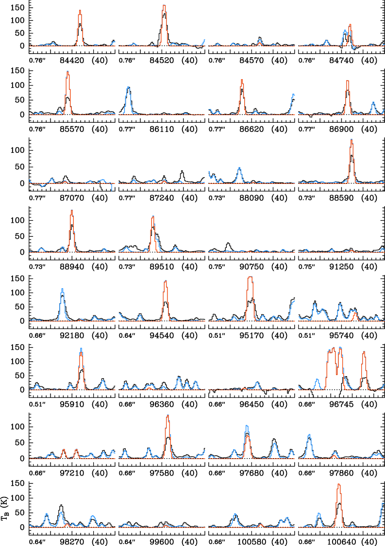
Figure 6: Transitions of CH₃OH, $\varv_{\rm t}=0$ covered by our ALMA survey. The best-fit LTE synthetic spectrum of CH₃OH, $\varv_{\rm t}=0$ is displayed in red and overlaid on the observed spectrum of Sgr B2(N1S), shown in black. The blue synthetic spectrum contains the contributions from all molecules identified in our survey so far, including from the species shown in red. The central frequency and width are indicated in MHz below each panel. The angular resolution (HPBW) is also indicated. The $y$-axis is labeled in brightness temperature units (K). The dotted line indicates the $3\sigma$ noise level.

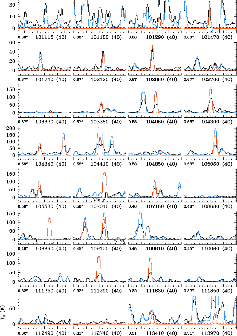
Figure 6: continued.

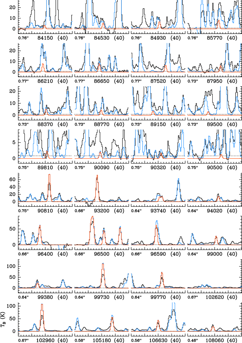
Figure 7: Same as Fig. 6, but for CH₃OH, $\varv_{\rm t}=1$.

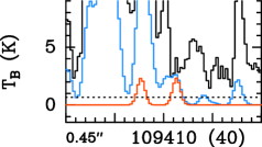
Figure 7: continued.

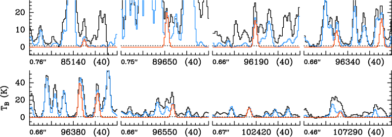
Figure 8: Same as Fig. 6, but for CH₃OH, $\varv_{\rm t}=2$.

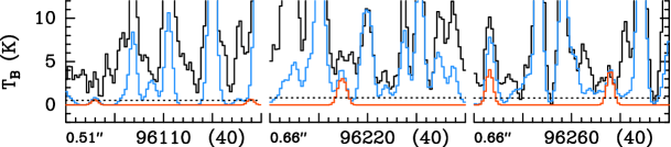
Figure 9: Same as Fig. 6, but for CH₃OH, $\varv_{\rm t}=3$.

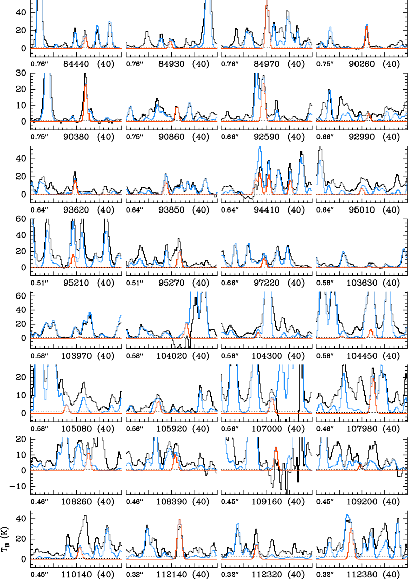
Figure 10: Same as Fig. 6, but for ¹³CH₃OH, $\varv_{\rm t}=0$.

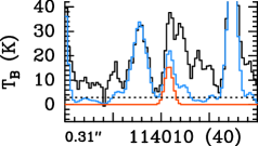
Figure 10: continued.

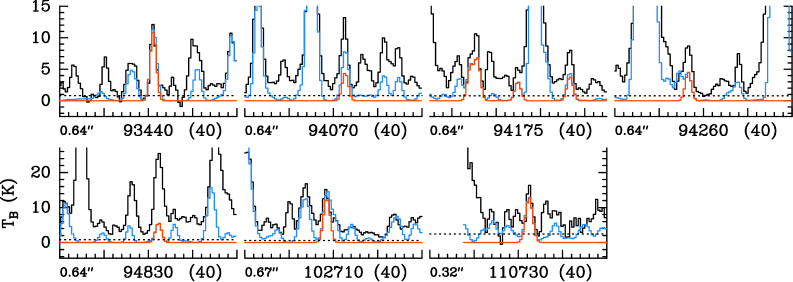
Figure 11: Same as Fig. 6, but for ¹³CH₃OH, $\varv_{\rm t}=1$.

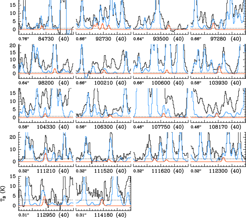
Figure 12: Same as Fig. 6, but for CH₃¹⁸OH, $\varv_{\rm t}=0$.

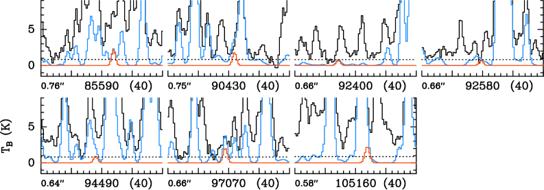
Figure 13: Same as Fig. 6, but for CH₃¹⁸OH, $\varv_{\rm t}=1$.

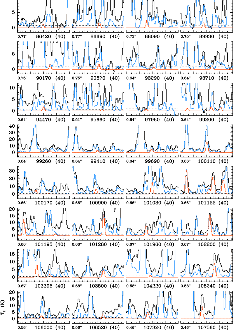
Figure 14: Same as Fig. 6, but for CH₃SH, $\varv_{\rm t}=0$.

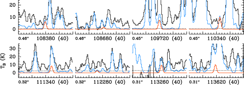
Figure 14: continued.

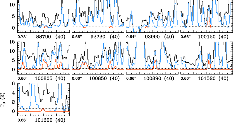
Figure 15: Same as Fig. 6, but for CH₃SH, $\varv_{\rm t}=1$.

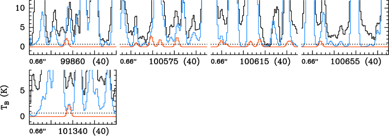
Figure 16: Same as Fig. 6, but for CH₃SH, $\varv_{\rm t}=2$.

Appendix C Complementary figures: Population diagrams

Figures 17–20 show population diagrams of methanol, its isotopologs, and methanethiol derived from the ReMoCA survey toward Sgr B2(N1S).

Figure 17: Population diagram of CH₃OH toward Sgr B2(N1S). The observed data points are shown in various colors (but not red), as indicated in the upper right corner of panel a, and the synthetic populations are shown in red. No correction is applied in panel a. In panel b, the optical depth correction has been applied to both the observed and synthetic populations, and the contamination by all other species included in the full model has been removed from the observed data points. The purple line is a linear fit to the observed populations (in linear-logarithmic space).

Figure 18: Same as Fig. 17, but for ¹³CH₃OH.

Figure 19: Same as Fig. 17, but for CH₃¹⁸OH.

Figure 20: Same as Fig. 17, but for CH₃SH.