Mass calibration of distant SPT galaxy clusters through expanded weak lensing follow-up observations with HST, VLT & Gemini-South

Abstract

Expanding from previous work we present weak lensing measurements for a total sample of 30 distant ($z_{\mathrm{median}}=0.93$) massive galaxy clusters from the South Pole Telescope Sunyaev-Zel’dovich (SPT-SZ) Survey, measuring galaxy shapes in Hubble Space Telescope (HST) Advanced Camera for Surveys images. We remove cluster members and preferentially select $z\gtrsim 1.4$ background galaxies via $V-I$ colour, employing deep photometry from VLT/FORS2 and Gemini-South/GMOS. We apply revised calibrations for the weak lensing shape measurements and the source redshift distribution to estimate the cluster masses. In combination with earlier Magellan/Megacam results for lower-redshifts clusters we infer refined constraints on the scaling relation between the SZ detection significance and the cluster mass, in particular regarding its redshift evolution. The mass scale inferred from the weak lensing data is lower by a factor $0.76^{+0.10}_{-0.14}$ (at our pivot redshift $z=0.6$) compared to what would be needed to reconcile a flat Planck $\nu\Lambda$CDM cosmology (in which the sum of the neutrino masses is a free parameter) with the observed SPT-SZ cluster counts. In order to sensitively test the level of (dis-)agreement between SPT clusters and Planck, further expanded weak lensing follow-up samples are needed.

1 Introduction

Massive galaxy clusters trace the densest regions of the cosmic large-scale structure. Robust constraints on their number density as a function of mass and redshift provide a powerful route to constrain the growth of structure and thereby cosmological parameters (e.g. Allen, Evrard & Mantz, 2011; Mantz et al., 2015; Dodelson et al., 2016; Bocquet et al., 2019). For this endeavour to be successful we not only need large cluster samples that have a well-characterised selection function, but also accurate mass measurements.

Suitable cluster samples are now in place, where one particularly powerful technique is provided by the Sunyaev-Zel’dovich (SZ, Sunyaev & Zel’dovich, 1970, 1972) effect. This effect describes a characteristic spectral distortion of the cosmic microwave background (CMB), caused by inverse Compton scattering of CMB photons off the electrons in the hot intra-cluster plasma. SZ surveys do not suffer from cosmic dimming, which is why high-resolution wide-area surveys, such as the ones conducted by the South Pole Telescope (SPT, Carlstrom et al., 2011) and the Atacama Cosmology Telescope (ACT, Swetz et al., 2011), have delivered large samples of massive clusters that extend out to the highest redshifts where these clusters exist (Bleem et al., 2015, 2020; Hilton et al., 2018, 2021; Huang et al., 2020). As a further benefit, the SZ signal provides a mass proxy with a comparably low intrinsic scatter ($\sim 20\%$, e.g. Angulo et al., 2012), which reduces the impact residual uncertainties regarding the selection function have on the cosmological parameter estimation.

Accurate cluster cosmology constraints require a careful calibration of mass-observable scaling relations. As a key ingredient, weak lensing (WL) observations provide the most direct route to obtain the absolute calibration of these relations (e.g. Allen, Evrard & Mantz, 2011). So far, the majority of constraints have been obtained for clusters at low and intermediate redshifts ($z\lesssim 0.6$) using ground-based WL data (e.g. von der Linden et al., 2014; Hoekstra et al., 2015; Okabe & Smith, 2016; McClintock et al., 2019; Miyatake et al., 2019; Stern et al., 2019; Umetsu et al., 2020; Herbonnet et al., 2020). However, cluster properties may evolve with redshift, making it imperative to extend the empirical WL mass calibration to higher redshifts. For higher-redshift clusters deeper imaging with higher resolution is required in order to resolve the typically small and faint distant background galaxies for WL shape measurements. Stacked analyses of large samples can still yield sensitive WL constraints for clusters out to $z\sim 1$ when using very deep optical images obtained from the ground over wide areas under excellent seeing conditions (Murata et al., 2019). However, in order to achieve tight measurements for rare high-mass, high-redshift clusters, even deeper data are needed, as provided e.g. by the Hubble Space Telescope (HST, see e.g. Jee et al., 2011, 2017; Thölken et al., 2018; Kim et al., 2019).

In the context of SPT, Schrabback et al. (2018a, S18 henceforth) presented a WL analysis of 13 distant ($0.57\leq z\leq 1.13$) galaxy clusters from the SPT-SZ survey (Bleem et al., 2015), using mosaic HST/ACS imaging for galaxy shape measurements. Dietrich et al. (2019, D19 henceforth) combined the resulting HST WL constraints with Magellan WL measurements of SPT-SZ clusters at lower redshifts in order to constrain X-ray and SZ mass-observable scaling relations. The same combined WL sample has been employed by Bocquet et al. (2019, B19 henceforth) to derive first directly WL-calibrated constraints on cosmology from the SPT-SZ cluster sample.

Here we update the S18 analysis and present results for an expanded sample. For the clusters in the S18 sample we report updated constraints, employing updated calibrations for WL shape estimates (Hernández-Martín et al., 2020, H20 henceforth) and the source redshift distribution (Raihan et al., 2020, R20 henceforth), and incorporating deeper VLT/FORS2 photometry for the source selection for six clusters. To this we add new measurements for 16 intermediate-mass clusters with single-pointing ACS F606W imaging and Gemini-South GMOS photometry plus one relaxed cluster with mosaic HST/ACS F606W+F814W imaging.

As the primary goal, our measurements aim at improving the mass calibration for high-redshift SPT clusters, thereby tightening constraints on the redshift-evolution of the SZ-mass scaling relation. This is particularly important in order to improve dark energy constraints based on the SPT-SZ cluster sample: as demonstrated by B19, constraints on the dark energy equation of state parameter $w$ show a strong degeneracy with the parameter $C_{\mathrm{SZ}}$, which describes the redshift evolution of the SZ-mass scaling relation. In order to improve the $w$ constraints we therefore need to tighten the constraints on $C_{\mathrm{SZ}}$ by adding WL data over a broad cluster redshift range.

This paper is organised as follows: We describe the data and image reduction in Sect. 2, followed by the photometric analysis and weak lensing measurements in Sect. 3. After presenting the weak lensing results in Sect. 4, we use these to derive revised constraints on the SPT observable–mass scaling relation in Sect. 5. We summarise our findings and conclude in Sect. 6.

Unless noted differently we assume a standard flat $\Lambda$CDM cosmology in this paper, characterised by $\Omega_{\mathrm{m}}=0.3$, $\Omega_{\Lambda}=0.7$, and $H_{0}=70\,h_{70}\mathrm{km/s/Mpc}$ with $h_{70}=1$, as approximately consistent with CMB constraints (e.g. Hinshaw et al., 2013; Planck Collaboration et al., 2020a). We additionally assume $\sigma_{8}=0.8$, $\Omega_{\mathrm{b}}=0.046$, and $n_{\mathrm{s}}=0.96$ when estimating the noise caused by large-scale structure projections for weak lensing mass estimates, as well as the computation of the concentration–mass relation according to Diemer & Joyce (2019). The term $\nu\Lambda$CDM denotes a flat $\Lambda$CDM cosmology in which the sum of the neutrino masses is treated as a free parameter. Transverse separations listed in this paper are physical distances, not comoving ones. All magnitudes are in the AB system and corrected for extinction according to Schlegel, Finkbeiner & Davis (1998). The (multivariate) normal distribution with mean $\mu$ and covariance matrix $\mathbf{\Sigma}$ is written as $\mathcal{N}(\mu,\mathbf{\Sigma})$.

2 Sample, data and data reduction

Table 1: Basic properties of the clusters with mosaic ACS imaging.

Cluster name	$z_{\mathrm{l}}$	$\xi$	Centre coordinates [deg J2000]				$M_{\mathrm{500c,SZ}}$	Sample/Data
			SZ $\alpha$	SZ $\delta$	X-ray $\alpha$	X-ray $\delta$	[$10^{14}\mathrm{M}_{\odot}h_{70}^{-1}$]
SPT-CL $J$0000$-$5748	0.702	8.49	0.2499	$-57.8064$	0.2518	$-57.8094$	$4.33^{+0.65}_{-0.86}$	S18 + new VLT
SPT-CL $J$0102$-$4915	0.870	39.91	15.7294	$-49.2611$	15.7350	$-49.2667$	$13.15^{+2.08}_{-2.83}$	S18
SPT-CL $J$0533$-$5005	0.881	7.08	83.4009	$-50.0901$	83.4018	$-50.0969$	$3.75^{+0.59}_{-0.82}$	S18 + new VLT
SPT-CL $J$0546$-$5345	1.066	10.76	86.6525	$-53.7625$	86.6532	$-53.7604$	$4.85^{+0.74}_{-1.04}$	S18
SPT-CL $J$0559$-$5249	0.609	10.64	89.9251	$-52.8260$	89.9357	$-52.8253$	$5.33^{+0.80}_{-0.95}$	S18
SPT-CL $J$0615$-$5746	0.972	26.42	93.9650	$-57.7763$	93.9652	$-57.7788$	$9.67^{+1.58}_{-2.16}$	S18
SPT-CL $J$2040$-$5725	0.930	6.24	310.0573	$-57.4295$	310.0631∗	$-57.4287^{*}$	$3.35^{+0.60}_{-0.81}$	S18 + new VLT
SPT-CL $J$2043$-$5035	0.723	7.18	310.8284	$-50.5938$	310.8244	$-50.5930$	$4.38_{-0.91}^{+0.72}$	new HST
SPT-CL $J$2106$-$5844	1.132	22.22	316.5206	$-58.7451$	316.5174	$-58.7426$	$7.76^{+1.19}_{-1.84}$	S18
SPT-CL $J$2331$-$5051	0.576	10.47	352.9608	$-50.8639$	352.9610	$-50.8631$	$5.17^{+0.75}_{-0.93}$	S18
SPT-CL $J$2337$-$5942	0.775	20.35	354.3523	$-59.7049$	354.3516	$-59.7061$	$7.67^{+1.14}_{-1.46}$	S18 + new VLT
SPT-CL $J$2341$-$5119	1.003	12.49	355.2991	$-51.3281$	355.3009	$-51.3285$	$5.30^{+0.82}_{-1.09}$	S18 + new VLT
SPT-CL $J$2342$-$5411	1.075	8.18	355.6892	$-54.1856$	355.6904	$-54.1838$	$3.86^{+0.64}_{-0.88}$	S18
SPT-CL $J$2359$-$5009	0.775	6.68	359.9230	$-50.1649$	359.9321	$-50.1697$	$3.54^{+0.61}_{-0.76}$	S18 + new VLT

Note. — Basic data from McDonald et al. (2013), Bleem et al. (2015), Chiu et al. (2016), and B19 for the 14 clusters with mosaic HST imaging included in this weak lensing analysis. Column 1: Cluster designation. Column 2: Spectroscopic cluster redshift. Column 3: Peak signal-to-noise ratio of the SZ detection. Columns 4–7: Right ascension $\alpha$ and declination $\delta$ of the SZ peak and X-ray centroid. ^∗: X-ray centroid from XMM-Newton data, otherwise Chandra. Column 8: SZ-inferred mass from B19, fully marginalising over cosmology and scaling relation parameter uncertainties. Column 9: Here we indicate the use of new HST or VLT data and whether the cluster was already included in the S18 analysis.

Table 2: Basic properties of the clusters with single-pointing ACS imaging.

Cluster name	$z_{\mathrm{l}}$	$\xi$	SZ peak position		$M_{\mathrm{500c,SZ}}$
			$\alpha$ [deg J2000]	$\delta$ [deg J2000]	[$10^{14}\mathrm{M}_{\odot}h_{70}^{-1}$]
SPT-CL $J$0044$-$4037	$1.02\pm 0.09$	4.92	11.1232	$-40.6282$	$2.80_{-0.80}^{+0.58}$
SPT-CL $J$0058$-$6145	$0.82\pm 0.03$	7.52	14.5799	$-61.7635$	$4.27_{-0.91}^{+0.70}$
SPT-CL $J$0258$-$5355	$0.99\pm 0.09$	4.96	44.5227	$-53.9233$	$2.88_{-0.80}^{+0.54}$
SPT-CL $J$0339$-$4545	$0.86\pm 0.03$	5.34	54.8908	$-45.7535$	$3.01_{-0.78}^{+0.57}$
SPT-CL $J$0344$-$5452	$1.05\pm 0.09$	7.98	56.0922	$-54.8794$	$4.02_{-0.93}^{+0.67}$
SPT-CL $J$0345$-$6419	$0.94\pm 0.03$	5.54	56.2510	$-64.3326$	$3.08_{-0.79}^{+0.64}$
SPT-CL $J$0346$-$5839	$0.70\pm 0.04$	4.83	56.5733	$-58.6531$	$2.92_{-0.77}^{+0.56}$
SPT-CL $J$0356$-$5337	$1.036$	6.02	59.0855	$-53.6331$	$3.21_{-0.81}^{+0.62}$
SPT-CL $J$0422$-$4608	$0.66\pm 0.04$	5.05	65.7490	$-46.1436$	$3.05_{-0.78}^{+0.59}$
SPT-CL $J$0444$-$5603	$0.94\pm 0.03$	5.18	71.1136	$-56.0576$	$2.91_{-0.77}^{+0.55}$
SPT-CL $J$0516$-$5755	$0.97\pm 0.03$	5.73	79.2398	$-57.9167$	$3.05_{-0.77}^{+0.58}$
SPT-CL $J$0530$-$4139	$0.78\pm 0.05$	6.19	82.6754	$-41.6502$	$3.92_{-0.89}^{+0.68}$
SPT-CL $J$0540$-$5744	$0.761$	6.74	85.0043	$-57.7405$	$3.67_{-0.78}^{+0.62}$
SPT-CL $J$0617$-$5507	$0.95\pm 0.09$	5.53	94.2808	$-55.1321$	$3.23_{-0.85}^{+0.63}$
SPT-CL $J$2228$-$5828	$0.73\pm 0.05$	5.15	337.2153	$-58.4686$	$3.27_{-0.83}^{+0.63}$
SPT-CL $J$2311$-$5820	$0.93\pm 0.09$	5.72	347.9924	$-58.3452$	$2.97_{-0.74}^{+0.60}$

Note. — Basic data from B19 for the SNAP clusters with single-pointing ACS imaging included in this weak lensing analysis. Column 1: Cluster designation. Column 2: Cluster redshift. Photometric (spectroscopic) redshifts are indicated with (without) error-bars. Column 3: Peak signal-to-noise ratio of the SZ detection. Columns 4–5: Right ascension $\alpha$ and declination $\delta$ of the SZ peak location. Column 6: SZ-inferred mass from B19, fully marginalising over cosmology and scaling relation parameter uncertainties.

All targets of our weak lensing analysis originate from the 2,500 deg² SPT-SZ galaxy cluster survey (Bleem et al., 2015). Here we employ updated cluster redshift estimates (see Tables 1 and 2 for a summary of basic properties) from Bayliss et al. (2016) and B19.

2.1 HST/ACS observations

2.1.1 High-mass clusters with ACS mosaics

S18 presented a weak lensing analysis for 13 high-redshift SPT-SZ clusters. They measured galaxy shapes in $2\times 2$ HST/ACS F606W mosaic images (1.92ks per pointing) and incorporated HST/ACS F814W imaging for the source selection (a single central F814W pointing for all clusters plus a $2\times 2$ mosaic for SPT-CL $J$0615$-$5746). We include these clusters in our analysis, where we apply updated shape and redshift calibrations for the source galaxies for all clusters (see Sect. 3), and additionally incorporate deeper VLT/FORS2 $I_{\mathrm{FORS2}}$ band imaging for the source selection for six of the clusters (see Sect. 2.2). We refer readers to S18 for details on the original data sets and analysis for these clusters, and primarily describe changes compared to this earlier analysis in the current work.

With SPT-Cl $J$2043$-$5035 we include a further cluster with $2\times 2$ HST/ACS mosaics in our analysis. This target was observed as part of a joint Chandra+HST programme (HST programme ID 14352, PI: J. Hlavacek-Larrondo, see also McDonald et al., 2019), which has obtained imaging in both F606W (1.93ks per pointing) and F814W (1.96ks per pointing). For this cluster we also incorporate central single pointing HST/ACS F606W imaging (1.44ks) obtained as part of the SPT ACS Snapshot Survey (SNAP 13412, PI: T. Schrabback).

2.1.2 Intermediate-mass clusters with single-pointing ACS imaging

From the SPT ACS Snapshot Survey (see Sect. 2.1.1) we additionally incorporate single pointing ACS F606W imaging for an additional 16 SPT-SZ clusters. These observations have total integration times between 1.44ks and 2.32ks (see Table 4), depending on cluster redshift and orbital visibility. These clusters have lower SZ detection significances and are therefore expected to be less massive compared to most of the clusters with mosaic ACS data (compare Tables 1 and 2), leading to a smaller physical extent (e.g. in terms of the radius $r_{\mathrm{500c}}$, within which the average density is 500 times the critical density of the Universe at the cluster redshift). While not ideal, the limited radial coverage provided by single-pointing ACS data is therefore still acceptable for these lower mass systems.

2.1.3 HST data reduction

For all data sets the observations were split into four exposures per pointing and filter, in order to facilitate good cosmic ray removal. We employ CALACS for basic image reductions, except for the correction for charge-transfer inefficiency (CTI), which is done using the method developed by Massey et al. (2014). For further image reductions we employ scripts from Schrabback et al. (2010) for the image registration and optimisation of masks and weights, as well as MultiDrizzle (Koekemoer et al., 2003) for the cosmic ray removal and stacking (see S18 for further details).

2.2 VLT/FORS2 observations

For six of the clusters initially studied by S18 we incorporate new VLT/FORS2 imaging obtained in the I_BESS+77 filter (which we call $I_{\mathrm{FORS2}}$) via programmes 0100.A-0217 (PI: B. Hernández-Martín), 0101.A-0694 (PI: H. Zohren), and 0102.A-0189 (PI: H. Zohren) into our analysis. These new observations are significantly deeper and have a better image quality (see Table 3) compared to the VLT data used by S18, thereby allowing us to include fainter source galaxies in the weak lensing analysis (see Sect. 3). Following S18 we reduce the new VLT images using theli (Erben et al., 2005; Schirmer, 2013), where we apply bias and flat-field corrections, relative photometric calibration, and sky background subtraction employing SExtractor (Bertin & Arnouts, 1996). We do not include the earlier shallower observations in the stack for two reasons. First, their inclusion would typically degrade the image quality in the stack given their looser image quality requirements. Additionally, they suffer from flat-field uncertainties (Moehler et al., 2010), which have been fixed prior to the new observations via an exchange of the FORS2 longitudinal atmospheric dispersion corrector (LADC) prisms (Boffin, Moehler & Freudling, 2016).

Table 3: The new VLT/FORS2 $I_{\mathrm{FORS2}}$ imaging data for clusters in the “updated ACS+FORS2 sample”.

Cluster name	$t_{\mathrm{exp}}$	$I_{\mathrm{lim}}(0\aas@@fstack{\prime\prime}8)$	$2r_{\mathrm{f}}^{*}$
SPT-CL $J$0000$-$5748	10.6ks	27.3	0$\aas@@fstack{\prime\prime}$70
SPT-CL $J$0533$-$5005	8.4ks	27.3	0$\aas@@fstack{\prime\prime}$59
SPT-CL $J$2040$-$5726	7.3ks	27.1	0$\aas@@fstack{\prime\prime}$62
SPT-CL $J$2337$-$5942	7.1ks	27.3	0$\aas@@fstack{\prime\prime}$64
SPT-CL $J$2341$-$5119	6.6ks	27.4	0$\aas@@fstack{\prime\prime}$63
SPT-CL $J$2359$-$5009	6.8ks	27.4	0$\aas@@fstack{\prime\prime}$69

Note. — Details of the analysed VLT/FORS2 imaging data. Column 1: Cluster designation. Column 2: Total co-added exposure time. Column 3: $5\sigma$-limiting magnitude using 0$\aas@@fstack{\prime\prime}$8 apertures, computed by placing apertures at random field locations that do not overlap with detected objects. Column 4: Image Quality defined as $2\times$ the FLUX_RADIUS estimate of stellar sources from SExtractor.

Table 4: Properties of HST/ACS SNAP and Gemini-South GMOS $i_{\mathrm{GMOS}}$ imaging data for clusters in the “ACS+GMOS sample”.

Cluster name	$t_{\mathrm{exp}}^{\mathrm{ACS}}$	$t_{\mathrm{exp}}^{\mathrm{GMOS}}$	$i_{\mathrm{lim}}(1\aas@@fstack{\prime\prime}5)$	$2r_{\mathrm{f}}^{*}$
SPT-CL $J$0044$-$4037	2.1ks	6.2ks	26.2	0$\aas@@fstack{\prime\prime}$93
SPT-CL $J$0058$-$6145	2.3ks	6.7ks	25.8	0$\aas@@fstack{\prime\prime}$92
SPT-CL $J$0258$-$5355	2.3ks	6.2ks	26.0	0$\aas@@fstack{\prime\prime}$70
SPT-CL $J$0339$-$4545	2.1ks	4.8ks	26.0	0$\aas@@fstack{\prime\prime}$88
SPT-CL $J$0344$-$5452	2.3ks	5.6ks	25.4	0$\aas@@fstack{\prime\prime}$92
SPT-CL $J$0345$-$6419	2.3ks	5.6ks	26.1	0$\aas@@fstack{\prime\prime}$69
SPT-CL $J$0346$-$5839	1.4ks	5.4ks	25.9	0$\aas@@fstack{\prime\prime}$82
SPT-CL $J$0356$-$5337	2.3ks	5.2ks	26.0	0$\aas@@fstack{\prime\prime}$77
SPT-CL $J$0422$-$4608	1.4ks	5.2ks	25.9	0$\aas@@fstack{\prime\prime}$66
SPT-CL $J$0444$-$5603	2.3ks	7.9ks	25.9	0$\aas@@fstack{\prime\prime}$72
SPT-CL $J$0516$-$5755	2.3ks	5.2ks	25.8	0$\aas@@fstack{\prime\prime}$85
SPT-CL $J$0530$-$4139	1.4ks	5.0ks	26.1	0$\aas@@fstack{\prime\prime}$77
SPT-CL $J$0540$-$5744	1.4ks	5.9ks	25.8	0$\aas@@fstack{\prime\prime}$72
SPT-CL $J$0617$-$5507	2.3ks	5.2ks	26.0	0$\aas@@fstack{\prime\prime}$91
SPT-CL $J$2228$-$5828	2.3ks	5.4ks	25.8	0$\aas@@fstack{\prime\prime}$75
SPT-CL $J$2311$-$5820	1.4ks	5.6ks	25.9	0$\aas@@fstack{\prime\prime}$99

Note. — Details of the analysed ACS and Gemini-South GMOS imaging data. Column 1: Cluster designation. Column 2: Total co-added exposure time with ACS in F606W. Column 3: Total co-added exposure time with GMOS in $i_{\mathrm{GMOS}}$. Column 4: $5\sigma$-limiting magnitude using 1$\aas@@fstack{\prime\prime}$5 apertures, computed by placing apertures at random field locations that do not overlap with detected objects. Column 5: Image Quality defined as $2\times$ the FLUX_RADIUS estimate of stellar sources from SExtractor.

2.3 Gemini-South observations

We obtained Gemini-South GMOS $i$-band imaging via NOAO programmes 2014B-0338 and 2016B-0176 (PI: B. Benson) for a subset of the clusters observed by the SNAP programme. In our analysis we include observations of 16 clusters, which have been observed to the full depth under good conditions (see Table 4). Similarly to the VLT data we reduced the GMOS images using theli, where we included only the central GMOS chip in the stack as it covers most of the ACS area.

3 Analysis

3.1 Shape measurements

S18 measured WL galaxy shapes for the clusters with mosaic ACS plus FORS2 observations (“ACS+FORS2 sample”) from the ACS F606W images, employing SExtractor (Bertin & Arnouts, 1996) for object detection and deblending, and the KSB+ formalism (Kaiser, Squires & Broadhurst, 1995; Luppino & Kaiser, 1997; Hoekstra et al., 1998) for shape measurements as implemented by Erben et al. (2001) and Schrabback et al. (2007). They modelled the spatial and temporal variations of the ACS point-spread function (PSF) using principal component analysis as done by Schrabback et al. (2010). Here we apply the same pipeline to also measure galaxy shapes for the remaining clusters in our larger sample.

As a significant update we employ the revised calibration of our shape measurement pipeline from H20 for all of our targets. This calibration was derived using custom galsim (Rowe et al., 2015) image simulations that closely resemble our ACS data. H20 mimic our observations in terms of depth, detector characteristics and point-spread function, and, importantly, adjust the galaxy sample such that its measured distributions in magnitude, size, and signal-to-noise ratio, as well as the ellipticity dispersion, closely match the corresponding observed quantities of our magnitude- and colour-selected source sample. They also employ distributions of galaxy light profiles that approximately resemble our colour-selected source population. H20 derive an updated correction for noise bias, where they assume a power-law dependence on the KSB signal-to-noise ratio $S/N_{\mathrm{KSB}}$ (incorporating the KSB weight function, see Erben et al., 2001) similar to Schrabback et al. (2010). They also obtain corrections to account for selection bias, the impact of neighbours and faint sources below the detection threshold (see also Euclid Collaboration: Martinet et al., 2019), and the increased light contamination caused by cluster galaxies. They demonstrate that our pipeline does not suffer from significant non-linear multiplicative shear biases in the regime of non-weak shears, which can occur in the inner cluster regions. Furthermore, they show that galaxies with slightly lower signal-to-noise ratios $S/N_{\mathrm{flux}}>7$, defined via SExtractor parameters $S/N_{\mathrm{flux}}=\mathrm{FLUX\_AUTO/FLUXERR\_AUTO}$, can be robustly included in the analysis when their revised noise-bias calibration is applied. We therefore employ this updated cut to boost the source number density (for comparison, S18 used galaxies with $S/N_{\mathrm{flux}}>10$) and apply a bias correction

$$m_{1,\text{corr}} = -0.358\left(S/N_{\mathrm{KSB}}\right)^{-1.145}\,-0.042,$$

$$m_{2,\text{corr}} = -0.357\left(S/N_{\mathrm{KSB}}\right)^{-1.298}\,-0.042\,,$$ (1)

based on the H20 results to the components of the KSB+ ellipticity estimates $\epsilon_{\alpha}^{\mathrm{biased}}$ on a galaxy-by-galaxy basis, to obtain corrected ellipticity estimates

$$\epsilon_{\alpha}=\frac{\epsilon_{\alpha}^{\mathrm{biased}}}{1+m_{\alpha,\text{corr}}}\,,$$ (2)

which act as unbiased estimates of the reduced shear $g$

$$\langle\epsilon_{\alpha}\rangle=g_{\alpha}\,.$$ (3)

Varying various aspects of the simulations, H20 conclude that our fully calibrated KSB+ pipeline yields accurate estimates for the reduced shear $g$ with an estimated relative systematic uncertainty of $1.5\%$, which we therefore include in our systematic error budget.

When applying the same $S/N_{\mathrm{flux}}>10$ selection as S18 and considering the ACS-only colour selection, we find that the new calibration increases the reduced shear estimates for our galaxies on average by 3.5%. Several effects contribute to this shift in the shear calibration, where the largest contributions come from the updated noise-bias correction, as well as the corrections for selection bias and the impact of faint sources below the detection threshold. The previously employed calibration from S10 did not account for the latter two effects, and its source samples did not adequately reflect our colour-selected sample of mostly background galaxies, leading to the shift in the noise bias correction. We however stress that the shift in the shear calibration is still within the the 4% systematic shear calibration uncertainty, which was included in the S18 analysis to account for the limitations in the S10 shear calibration.

Additional changes in the (noisy) reduced shear profiles for the previously studied clusters occur due to the inclusion of galaxies with $7<S/N_{\mathrm{flux}}<10$, and the deeper photometric source selection in the case of clusters with new VLT data (see Sect. 3.2).

Note that Hoekstra et al. (2015) apply a bias calibration for their KSB+ implementation which is a function of both the galaxy signal-to-noise ratio and a resolution factor that depends on the half-light radii of the PSF and the galaxy. Capturing such a size dependence is less important for space-based data as variations in PSF size are much smaller compared to typical seeing-limited ground-based data. In addition, the variation in galaxy sizes is smaller in our case given the selection of mostly high-redshift galaxies via colour (see Sect. 3.2). H20 show that the residual multiplicative shear bias of our KSB+ implementation (after applying the $S/N_{\mathrm{KSB}}$-dependent correction) depends only weakly on the FLUX_RADIUS parameter $r_{\mathrm{f}}$ from SExtractor (within $\sim\pm 5\%$ for most of the galaxies). Combined with the weak dependence of the average geometric lensing efficiency on $r_{\mathrm{f}}$ for our colour- and magnitude-selected source sample (see Appendix A), we can therefore safely ignore second-order effects for the bias correction.

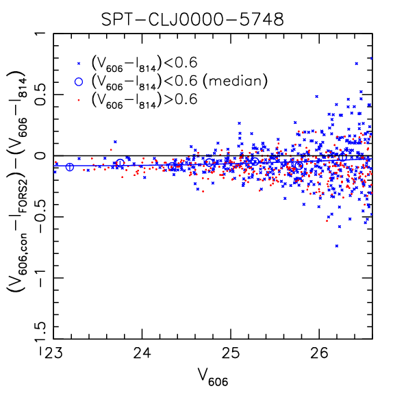
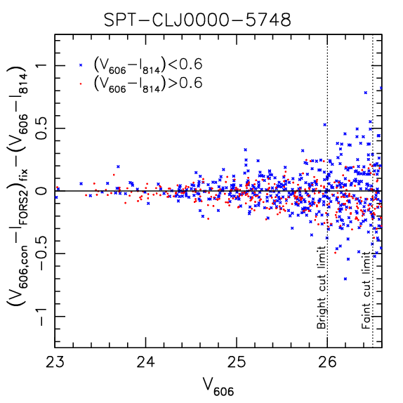
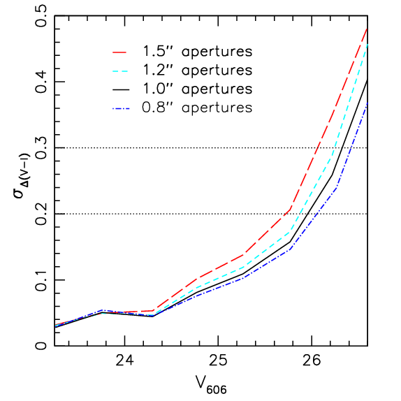
Figure 1: Left: Measured colour difference $\Delta(V-I)=(V_{606,\mathrm{con}}-I_{\mathrm{FORS2}})-(V_{606}-I_{814})$ between the PSF homogenised ACS+FORS2 colour estimate $V_{606,\mathrm{con}}-I_{\mathrm{FORS2}}$ (measured using 0$\aas@@fstack{\prime\prime}$8 apertures) and the ACS-only colour estimate $(V_{606}-I_{814})$ in the inner region of SPT-CL $J$0000$-$5748 as a function of $V_{606}$. Blue galaxies with $(V_{606}-I_{814})<0.6$ are shown as small blue crosses, while red galaxies with $(V_{606}-I_{814})>0.6$ are indicated as red points. The open circles show the median values for the blue galaxies in magnitude bins, where the (small) error-bars correspond to the uncertainty on the mean for a Gaussian distribution and the curve shows their best-fit second-order polynomial interpolation. Middle: Here we show the same data after subtraction of this function. The photometric scatter distribution for the ACS+FORS2 selection is sampled from this distribution of offsets. The vertical lines separate the magnitude ranges for the different colour cuts. Right: Scatter in the model-subtracted $\Delta(V-I)$ colour offsets as a function of $V_{606}$, averaged over all clusters listed in Table 3. The different curves correspond to different aperture diameters in the ACS+FORS2 analysis. The dotted horizontal lines indicate the scatter limits S18 employed to define the bright cut and faint cut in their colour selection.

3.2 Photometry and colour selection

As done by S18 we select weak lensing source galaxies via $V-I$ colour, allowing us to efficiently remove both red and blue cluster members (for clusters at redshifts $0.6\lesssim z_{\mathrm{l}}\lesssim 1$) as well as the majority of foreground galaxies, and keep most of the lensed background galaxies at $z\gtrsim 1.4$. For SPT-Cl $J$2043$-$5035 and the inner regions of the clusters with VLT observations (Table 3) we can directly employ $V_{606}-I_{814}$ colours measured in the HST/ACS data (“ACS-only” colours). Following S18 we here employ apertures with diameter 0$\aas@@fstack{\prime\prime}$7 to be consistent with the definitions of the photometric redshift catalogue from Skelton et al. (2014, see Sect. 3.4) and select $24<V_{606}<26$ galaxies with $V_{606}-I_{814}<0.3$ plus $26<V_{606}<26.5$ galaxies with $V_{606}-I_{814}<0.2$.

For the clusters in the ACS+GMOS sample (Table 4) as well as the outskirts of the clusters in the updated ACS+FORS2 sample (Table 3) we have to rely on PSF-homogenised colour measurements between the ACS F606W images and the ground-based $i_{\mathrm{GMOS}}$- or $I_{\mathrm{FORS2}}$-band images from Gemini-South/GMOS or VLT/FORS2, respectively. After homogenising the PSF we measure convolved aperture colours $V_{606,\mathrm{con}}-I_{\mathrm{FORS2}}$ and $V_{606,\mathrm{con}}-i_{\mathrm{GMOS}}$, respectively, using a range of aperture diameters.

For all data sets we employ conservative masks to remove regions near bright stars, very extended galaxies, and the image boundaries.

3.2.1 ACS+FORS2 analysis

For the ACS+FORS2 sample the following steps of the colour measurements and colour selection closely follow Appendix D of S18. Here we only describe the updated analysis for the clusters with new VLT observations. For the other ACS+FORS2 clusters the colour measurements and selections were described in S18 and have not been changed for this reanalysis.

In order to achieve a residual FORS2 zero-point calibration and a consistent colour selection between the $V_{606,\mathrm{con}}-I_{\mathrm{FORS2}}$ and $V_{606}-I_{814}$ colours we compute colour offsets

$$\Delta(V-I)=(V_{606,\mathrm{con}}-I_{\mathrm{FORS2}})-(V_{606}-I_{814})$$ (4)

for blue galaxies in the overlap region of the $I_{\mathrm{FORS2}}$ images and the central ACS F814W images (see the left panel of Fig. 1 for an example). We then fit the median of these offsets as a function of $V_{606}$ aperture magnitude using a second-order polynomial and subtract this model from the measured $V_{606,\mathrm{con}}-I_{\mathrm{FORS2}}$ colours, providing corrected colour estimates $(V_{606,\mathrm{con}}-I_{\mathrm{FORS2}})_{\mathrm{fix}}$ (see the middle panel of Fig. 1) not only in the inner cluster region, but also the full field covered by FORS2.

The right panel of Fig. 1 shows the measured scatter in $\Delta(V-I)$ as a function of $V_{606}$ magnitude after the model subtraction for different aperture diameters, averaged over the six clusters with new VLT data. This clearly shows that the 1$\aas@@fstack{\prime\prime}$5 apertures employed by S18 are not optimal for the new VLT data, which is a result of the excellent image quality of the new observations and the typically very small spatial extent of the faint blue galaxies constituting our source sample. For the ACS+FORS2 analysis of the clusters with new VLT data we therefore employ smaller apertures with diameter 0$\aas@@fstack{\prime\prime}$8, which significantly reduces the scatter in the colour differences to the ACS-only colours. Together with the longer FORS2 integration times this allows us to include fainter galaxies in the ACS+FORS2 colour selection compared to the S18 analysis, where we now select $24<V_{606}<26$ galaxies with $(V_{606,\mathrm{con}}-I_{\mathrm{FORS2}})_{\mathrm{fix}}<0.2$ (“bright cut” regime in the middle panel of Fig. 1) plus $26<V_{606}<26.5$ galaxies with $(V_{606,\mathrm{con}}-I_{\mathrm{FORS2}})_{\mathrm{fix}}<0.0$ (“faint cut” regime in the middle panel of Fig. 1).

When calibrating the source redshift distribution (see Sect. 3.4) we have to account for the impact of photometric scatter. To model the scatter compared to the ACS-only colours we then sample from the measured scatter distribution in $\Delta(V-I)$ for each cluster in the ACS+FORS2 sample (see the middle panel of Fig. 1 for an example), split into magnitude and colour bins as done by S18.

3.2.2 ACS+GMOS analysis

For the ACS+GMOS sample ACS F814W imaging is not available, which is why we cannot directly apply the same colour calibration scheme. Instead, we calibrate the colours via shallower Magellan/PISCO $griz$ photometry, which itself has been calibrated using stellar locus regression to the SDSS photometric system (corrected for galactic extinction, see Bleem et al., 2020).

For the cluster SPT-CL $J$0615$-$5746 both PISCO photometry and HST/ACS $V_{606}-I_{814}$ colours (from S18) are available, allowing us to calibrate the transformation

$$(V_{606}-I_{814})-(r-i)\simeq(0.222\pm 0.025)(g-i-1.0)+0.096\pm 0.014$$ (5)

using stars with $20<V_{606}<22$ and $g-i<2$. Alternative choices to include fainter stars or galaxies change the fit coefficients in Eq. 5 slightly, but affect the resulting transformed colour in the regime of our colour cuts by $\leq 0.01$ mag only, providing sufficient accuracy for our study.

Employing Eq. 5 we compute the transformed $V_{606}-I_{814}$ colours for the PISCO objects in the fields of the ACS+GMOS clusters. Using overlapping bright objects with $20<V_{606}<23$ from our ACS+GMOS photometry we then derive the required transformation from $V_{606,\mathrm{con}}-i_{\mathrm{GMOS}}$ to $V_{606}-I_{814}$. Here we first compute a linear fit $(V_{606}-I_{814})=a(V_{606,\mathrm{con}}-i_{\mathrm{GMOS}})+b$ between these colours for each cluster field separately. To reduce the sensitivity to outliers we then fix the slope to the median slope from all fields $a_{\mathrm{med}}=1.147\pm 0.013$ in a second step and redetermine $b$ using a median estimate for each cluster field, effectively providing the zero-point calibration for the GMOS data. Here we exclude very red objects ($V_{606}-I_{814}>1.2$) to optimise the calibration close to the regime of our colour cut.

As the final ingredient for the ACS+GMOS photometric analysis we need to obtain a model for the photometric scatter. Different to the ACS+FORS2 analysis we cannot derive this from the comparison of in-field ACS $V_{606}-I_{814}$ colour measurements. Instead, we make use of GMOS $i$-band imaging that we obtained for cross-calibration in the centre of the GOODS-South field with similar characteristics to our cluster fields (exposure time 5.0ks). For this field we can directly calibrate and compare to ACS $V_{606}-I_{814}$ colours similarly to the ACS+FORS2 analysis. We then apply the resulting magnitude- and colour-dependent photometric scatter distribution from this field as a scatter model in the redshift calibration of the ACS+GMOS clusters (see Sect. 3.4).

On average the image quality of our GMOS observations is significantly worse than for our new VLT observations (compare Tables 3 and 4). Following S18 we therefore employ 1$\aas@@fstack{\prime\prime}$5 apertures for the ACS+GMOS photometry. Thanks to the deep GMOS integration times we can still include $24<V_{606}<25.8$ galaxies in our analysis (selected via a cut $V_{606}-I_{814}<0.2$ in transformed colour), but we have to drop $V_{606}>25.8$ galaxies given their increased photometric scatter.

3.3 Number density checks

After accounting for masks, our colour and source selection results in average galaxy number densities within the weak lensing fit range (see Sect. 4.2) of 15.5/arcmin² for the ACS+FORS2 selection and 10.9/arcmin² for the ACS+GMOS selection (values not corrected for magnification, see Table 5 for the source densities of individual clusters).

An important consistency check for the source selection is provided by the number density profile of the selected sources. On average it should be consistent with flat if cluster members have been accurately removed and if the impact of masks and weak lensing magnification have been properly accounted for. Sources appear brighter due to magnification, which increases the source counts. However, at the depth of our data the change in solid angle has a bigger impact, leading to a net reduction in the measured source density (S18). To compensate for the impact of magnification, we follow S18 and employ the best-fit NFW reduced shear profile model for each cluster (see Sect. 4.2) to compute magnitude- and cluster redshift-dependent corrections for the source density profile and the estimate of the mean geometric lensing efficiency (see Sect. 3.4). These corrections were derived by S18 based on the magnitude-dependent source redshift distribution in CANDELS data.

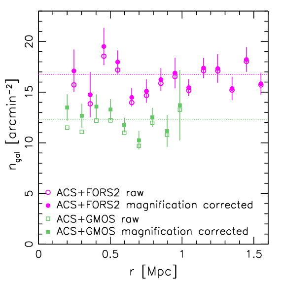
Figure 2: Weak lensing source density as a function of distance to the X-ray cluster centre for the ACS+FORS2 selection (magenta points) and the SZ cluster centre for the ACS+GMOS selection (green squares). The points show the average number density from all available fields (including only clusters with new FORS2 data in case of the ACS+FORS2 selection), where open symbols correspond to raw (mask-corrected) values, while filled symbols have additionally been corrected for magnification assuming the best-fit NFW cluster models (Sect. 4.2). The error-bars indicate the uncertainty on the mean for the magnification-corrected values as estimated from the dispersion between the different fields. They are correlated due to large-scale structure variations. Error-bars for the raw values have a similar size but are not shown for clarity. The horizontal lines correspond to the global average densities corrected for magnification.

As visible in Fig. 2, the corrected source density profile is consistent with flat for the ACS+FORS2 selection, as expected for an accurate cluster member removal. Within the uncertainty this is also the case for the ACS+GMOS selection (error-bars are correlated due to large-scale structure variations in the source population, especially at small radii), but here the limited radial range limits the constraining power of the test. As a further cross-check we therefore investigate the measured number counts of the colour-selected sources in the ACS+GMOS and ACS+FORS2 selected samples (which apply consistent source selections at brighter magnitudes) in Fig. 3. Their number counts do not only agree well with each other, but also with the expected number counts from the CANDELS fields, which have been degraded to the same noise properties. We therefore conclude that cluster members have been removed accurately. Note that our magnification correction does not account for miscentring of the cluster shear profile and mass distribution (see Sect. 4.3), likely leading to a minor over-correction at small radii. This effect should be more pronounced for the ACS+GMOS sample given the poorer SZ centre proxy. This could be the cause for the mild increase that is tentatively visible (within the errors) for the magnification-corrected ACS+GMOS number density profile in Fig. 2 at small radii.

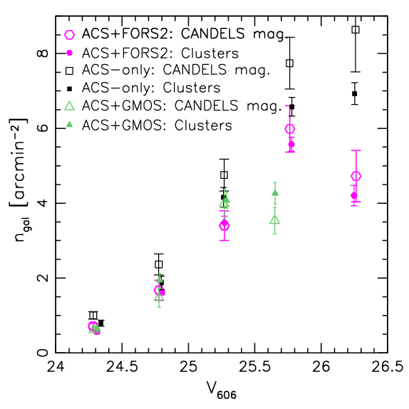
Figure 3: Number density of selected source galaxies $n_{\mathrm{gal}}$ as a function of $V_{606}$ magnitude, accounting for masks. Solid green triangles show the average source density in the ACS+GMOS data, while solid magenta hexagons and black squares correspond to the source densities for the ACS+FORS2 and ACS-only selections, respectively, averaged over the six cluster fields with new VLT/FORS2 imaging. The corresponding source density estimates from the CANDELS fields are shown with the large open symbols, applying a consistent selection, photometric scatter, and artificial magnification based on the best-fit cluster NFW models. The error-bars indicate the uncertainty on the mean as estimated from the variation between the contributing cluster fields or the five CANDELS fields, respectively, assuming Gaussian scatter. Errors are correlated between magnitude bins due to large-scale structure. Especially at faint magnitudes source densities differ between the selections due to their differences in depth and applied colour limits.

Table 5: Summary of geometric lensing efficiencies and source densities. The three sets of rows correspond the ACS mosaic clusters with new observations, ACS mosaic clusters without new observations, and clusters from the ACS+GMOS sample, respectively.

Cluster	$\langle\beta\rangle$	$\langle\beta^{2}\rangle$	$\sigma_{\langle\beta\rangle_{j}}/\langle\beta\rangle$	$n_{\mathrm{gal}}[\mathrm{arcmin^{-2}}]$
				ACS-only	ACS+FORS2/GMOS
SPT-CL $J$0000$-$5748	0.459	0.241	0.051	20.3	14.8
SPT-CL $J$0533$-$5005	0.372	0.163	0.061	20.7	16.9
SPT-CL $J$2040$-$5726	0.351	0.146	0.065	20.8	13.5
SPT-CL $J$2043$-$5035	0.441	0.226	0.073	20.2	-
SPT-CL $J$2337$-$5942	0.424	0.207	0.055	19.1	15.4
SPT-CL $J$2341$-$5119	0.323	0.124	0.069	21.3	14.8
SPT-CL $J$2359$-$5009	0.420	0.205	0.055	19.7	17.3
SPT-CL $J$0102$-$4915	0.370	0.163	0.072	20.4	4.0
SPT-CL $J$0546$-$5345	0.299	0.108	0.095	13.8	3.3
SPT-CL $J$0559$-$5249	0.496	0.284	0.065	18.7	3.8
SPT-CL $J$0615$-$5746	0.331	0.132	0.084	19.9	2.9
SPT-CL $J$2106$-$5844	0.275	0.092	0.103	9.8	2.2
SPT-CL $J$2331$-$5051	0.514	0.304	0.066	19.8	8.1
SPT-CL $J$2342$-$5411	0.294	0.104	0.097	15.2	2.6
SPT-CL $J$0044$-$4037	0.309	0.116	0.115	-	13.2
SPT-CL $J$0058$-$6145	0.393	0.182	0.105	-	12.4
SPT-CL $J$0258$-$5355	0.322	0.125	0.109	-	12.2
SPT-CL $J$0339$-$4545	0.376	0.167	0.109	-	11.5
SPT-CL $J$0344$-$5452	0.299	0.109	0.103	-	7.8
SPT-CL $J$0345$-$6419	0.343	0.140	0.104	-	10.8
SPT-CL $J$0346$-$5839	0.453	0.238	0.098	-	9.0
SPT-CL $J$0356$-$5337	0.300	0.111	0.112	-	12.0
SPT-CL $J$0422$-$4608	0.476	0.259	0.084	-	7.8
SPT-CL $J$0444$-$5603	0.344	0.141	0.105	-	10.7
SPT-CL $J$0516$-$5755	0.331	0.131	0.096	-	9.8
SPT-CL $J$0530$-$4139	0.412	0.199	0.106	-	12.4
SPT-CL $J$0540$-$5744	0.422	0.208	0.090	-	11.0
SPT-CL $J$0617$-$5507	0.335	0.136	0.116	-	10.9
SPT-CL $J$2228$-$5828	0.441	0.224	0.082	-	10.6
SPT-CL $J$2311$-$5820	0.349	0.144	0.099	-	12.9

Note. — Column 1: Cluster designation. Columns 2–4: $\langle\beta\rangle$, $\langle\beta^{2}\rangle$, and $\sigma_{\langle\beta\rangle_{j}}/\langle\beta\rangle$ averaged over both colour selection schemes and all magnitude bins that are included in the NFW fits according to their corresponding shape weight sum. Columns 5–6: Density of selected sources in the cluster fields for the ACS-only and the ACS+FORS2/GMOS colour selection schemes, respectively (averaged within the fit range and not corrected for magnification).

3.4 Calibration of the source redshift distribution

The weak lensing shear $\gamma$ and convergence $\kappa$ (see e.g. Schneider, 2006) scale with the average geometric lensing efficiency

$$\langle\beta\rangle=\frac{\sum\beta(z_{i})w_{i}}{\sum w_{i}}$$ (6)

of the sources galaxies, where $w_{i}$ is the shape weight of galaxy $i$, and

$$\beta=\mathrm{max}\left[0,\frac{D_{\mathrm{ls}}}{D_{\mathrm{s}}}\right]\,$$ (7)

is defined via the angular diameter distances $D_{\mathrm{s}}$, $D_{\mathrm{l}}$, and $D_{\mathrm{ls}}$ to the source, to the lens, and between lens and source, respectively. Since we have removed cluster members and other galaxies at or near the redshifts of the targeted clusters via the colour selection (see Sect. 3.2), there is no need to obtain individual photometric redshifts (photo-$z$s). Instead, we can infer the redshift distribution and therefore $\langle\beta\rangle$ via observations of well-studied reference fields, to which we apply a consistent source selection. For this purpose, S18 employed photo-$z$ catalogues computed by the 3D-HST team (Skelton et al., 2014, S14 henceforth) for the CANDELS fields (Grogin et al., 2011). The five CANDELS fields have not only been observed by HST with at least four imaging filters (including deep NIR, see Koekemoer et al., 2011) plus slitless spectroscopy (Momcheva et al., 2016), but they also benefit from a wide range of additional imaging and spectroscopic observations obtained with other facilities (see S14). Together with their significant sky coverage, which is needed to reduce the impact of sampling variance, this turns them into an outstanding reference sample to infer the redshift distribution for deep WL data (S18).

Through the comparison with even deeper photometric and spectroscopic redshifts (Rafelski et al., 2015; Brammer et al., 2012, 2013) available in the overlapping Hubble Ultra Deep Field, S18 showed that the S14 photo-$z$s nevertheless suffer from systematic issues such as catastrophic redshift outliers and redshift focusing effects (e.g. Wolf, 2009), which would bias the resulting cluster masses high by $\sim 12\%$ if unaccounted for. In order to achieve an initial correction for this effect, S18 introduced an approximate empirical scheme to statistically correct the S14 photo-$z$s for these effects. Recently, R20 revisited this issue, also including new ultra-deep spectroscopic data from MUSE (Inami et al., 2017) in the comparison. By varying both the inputs and the analysis scheme, R20 show that the bias in the inferred redshift distribution can be avoided by using BPZ (Benítez, 2000) instead of EAZY (Brammer, van Dokkum & Coppi, 2008), for which in particular BPZ’s template interpolation plays a crucial role. R20 compute BPZ photo-$z$s for the five CANDELS fields based on the HST photometry and a subset of the ground-based photometric data provided by S14. From their tests R20 conclude that their catalogues are expected to provide accurate $\langle\beta\rangle$ estimates for observations similar to our data within a total systematic uncertainty of 3.0%, which accounts for the impact of residual systematic photo-$z$ uncertainties and sampling variance. Recomputing the S18 WL cluster mass constraints using their updated CANDELS catalogues for the redshift calibration, R20 find that the masses shift by $\sim+1\%$ only compared to the S18 results. This good agreement is an important confirmation of the robustness of the results, given that both approaches should provide unbiased $\langle\beta\rangle$ estimates within their systematic uncertainties. The joint uncertainty quoted by S18 for photo-$z$ uncertainties and sampling variance (2.4%) is slightly smaller, but this ignores the impact depth variations between the different CANDELS fields have on the systematic biases and uncertainties. In contrast, this issue has been investigated by R20 via the degradation of higher quality data and it is effectively accounted for in their analysis via their full photo-$z$ re-computation. We therefore use the R20 CANDELS photo-$z$s as the redshift calibration reference sample for our analysis.

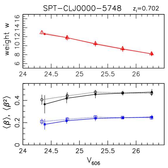
Figure 4: Dependence of different parameters in the analysis of SPT-CL $J$0000$-$5748 on $V_{606}$ magnitude. Small solid (large open) symbols correspond to the analysis using ACS-only (ACS+FORS2) colours. Top: Average weak lensing shape weight $w$, where the error-bars show the dispersion from all selected galaxies in the magnitude bin. Bottom: $\langle\beta\rangle$ (circles) and $\langle\beta^{2}\rangle$ (squares), where the error-bars correspond to the dispersion of their estimates between the cluster-field-sized CANDELS sub-patches.

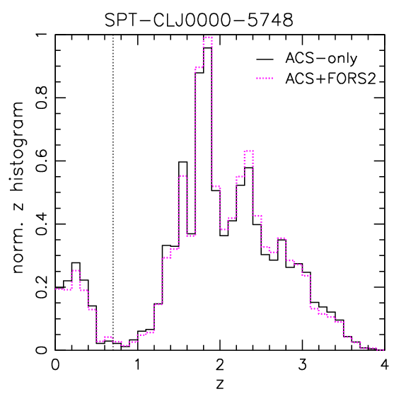
Figure 5: Inferred average redshift distribution of source galaxies using the ACS-only versus ACS+FORS2 colour selection for data with the noise properties of our observations of SPT-CL $J$0000$-$5748, based on the CANDELS photometric redshift catalogues from R20.

In order to compute $\langle\beta\rangle$ we first match the noise properties for the magnitude and $V_{606}-I_{814}$ colour selection between the corresponding cluster field and the CANDELS data as done by S18, employing the photometric scatter distributions described in Sections 3.2.1 and 3.2.2 for the ACS+FORS2 and ACS+GMOS analyses, respectively. Following the colour and magnitude selection we then compute $\langle\beta\rangle$ from the CANDELS catalogues in 0.5mag-wide $V_{606}$ magnitude bins (see Fig. 4) to improve the weighting and tighten the overall constraints (see Sect. 4.2 and Table 5 for effective joint values). We likewise compute $\langle\beta^{2}\rangle(V_{606})$ to account for the impact of the broad width of the redshift distribution following Seitz & Schneider (1997); Hoekstra, Franx & Kuijken (2000) and Applegate et al. (2014). In addition to obtaining global best estimates for the mean redshift distribution (see Fig. 5 for an example) and $\langle\beta\rangle(V_{606})$, we also estimate the line-of-sight scatter $\sigma_{\langle\beta\rangle_{j}}$ by placing apertures $j$ of the size of our corresponding cluster-field observations into the CANDELS fields (see S18).

The total systematic uncertainty in the $\langle\beta\rangle$ estimates comprises the 3.0% uncertainty estimate from R20, and in addition minor contributions from deblending differences and potential residual contamination of the source sample by very blue cluster members. For the latter, we use the estimates from S18 of 0.5% and 0.9%, respectively, yielding a joint uncertainty of 3.2% (added in quadrature).

4 Weak lensing results

Table 6: Locations ($\alpha,\delta$) of the peaks in the mass reconstruction signal-to-noise ratio maps, their positional uncertainty ($\Delta\alpha,\Delta\delta$) as estimated by bootstrapping the galaxy catalogue, and their peak signal-to-noise ratio $(S/N)_{\mathrm{peak}}$. Here we only include clusters with new observations and $(S/N)_{\mathrm{peak}}>1.5$. The top set of rows includes clusters with ACS mosaics, while the bottom set includes clusters from the ACS+GMOS sample.

Cluster	$\alpha$	$\delta$	$\Delta\alpha$	$\Delta\delta$	$\Delta\alpha$	$\Delta\delta$	$(S/N)_{\mathrm{peak}}$
	[deg J2000]	[deg J2000]	[arcsec]	[arcsec]	[kpc]	[kpc]
SPT-CL $J$0000$-$5748	0.25607	$-57.80996$	2.7	2.4	20	17	5.4
SPT-CL $J$0533$-$5005	83.39302	$-50.10844$	7.8	7.1	61	55	3.3
SPT-CL $J$2040$-$5725	310.05696	$-57.42120$	4.7	7.0	37	55	3.4
SPT-CL $J$2043$-$5035	310.81687	$-50.59325$	4.3	7.8	31	56	3.3
SPT-CL $J$2337$-$5942	354.35873	$-59.70801$	1.1	1.3	8	9	7.0
SPT-CL $J$2341$-$5119	355.30057	$-51.32996$	2.1	3.4	17	27	3.8
SPT-CL $J$2359$-$5009	359.93212	$-50.16927$	3.6	5.1	27	38	4.8
SPT-CL $J$0058$-$6145	14.58664	$-61.76796$	2.7	2.1	20	16	4.3
SPT-CL $J$0258$-$5355	44.52738	$-53.92520$	3.5	3.3	28	27	4.0
SPT-CL $J$0339$-$4545	54.87871	$-45.75065$	11.0	5.7	84	44	2.2
SPT-CL $J$0345$-$6419	56.25103	$-64.33496$	9.9	6.4	78	51	2.5
SPT-CL $J$0346$-$5839	56.57704	$-58.65087$	4.6	4.2	33	30	3.5
SPT-CL $J$0356$-$5337	59.09500	$-53.63168$	11.4	10.5	92	85	1.6
SPT-CL $J$0422$-$4608	65.73875	$-46.14217$	2.6	3.2	18	23	4.3
SPT-CL $J$0444$-$5603	71.10803	$-56.05631$	6.4	5.3	51	42	3.0
SPT-CL $J$0516$-$5755	79.25988∗	$-57.89916^{*}$	4.2	6.6	33	52	3.4
SPT-CL $J$0530$-$4139	82.67820	$-41.65160$	5.6	2.9	41	21	3.6
SPT-CL $J$0540$-$5744	84.99319	$-57.74324$	6.2	7.8	45	57	3.3
SPT-CL $J$0617$-$5507	94.27795	$-55.13300$	7.8	7.9	62	62	2.7
SPT-CL $J$2228$-$5828	337.17934	$-58.47028$	7.7	12.8	56	93	2.5
SPT-CL $J$2311$-$5820	347.99784∗	$-58.36331^{*}$	10.4	10.2	81	81	2.5

Note. — ^∗: Indicates a less reliable peak close to the edge of the field of view.

4.1 Mass reconstructions

The weak lensing shear $\gamma$ and convergence $\kappa$, which are linked to the reduced shear as

$$g=\frac{\gamma}{1-\kappa}\,,$$ (8)

are both second-order derivatives of the lensing potential (e.g. Bartelmann & Schneider, 2001). Therefore, it is possible to reconstruct the convergence field from the shear field up to a constant, which is the mass-sheet degeneracy (Kaiser & Squires, 1993; Schneider & Seitz, 1995). Following S18 we employ a Wiener-filtered reconstruction algorithm (McInnes et al., 2009; Simon, Taylor & Hartlap, 2009), which also has the advantage of properly accounting for the spatially varying source densities in our ACS+FORS2 data sets. We fix the mass-sheet degeneracy by setting the average convergence inside each cluster field to zero. While this generally leads to an underestimation of $\kappa$, this is a relatively minor effect for the clusters with ACS mosaics. The impact is bigger for the clusters in the ACS+GMOS sample given the smaller field-of-view, but note that we only use the mass reconstructions for illustrative purposes and not for quantitative mass constraints.

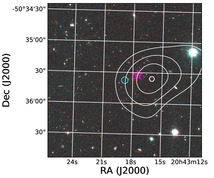
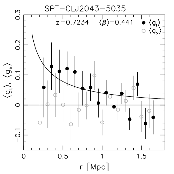
Figure 12: WL results for SPT-CL $J$2043$-$5035. Left: Signal-to-noise ratio map of the WL mass reconstruction (starting at $2\sigma$ in steps of $0.5\sigma$, with the peak indicated by the hexagon), overlaid on the ACS F606W/F814W mosaic image ($2\aas@@fstack{\prime}5\times 2\aas@@fstack{\prime}5$ cutout, using F814W for the red channel and F606W for the blue and green channels). The BCG (from McDonald et al., 2019), SZ peak, and X-ray centroid are shown by the magenta star, cyan circle, and red square, respectively. Right: Combined reduced shear profile around the X-ray centre, showing the tangential (black solid circles with best-fitting NFW model) and cross (grey open circles, shifted along the $x$-axis for clarity) components.

The left panels of Figs. 12 to 20 show mass signal-to-noise ratio ($S/N$) contours overlaid on colour images for all clusters in our sample with new observations. To compute the $S/N$ maps we generate 500 noise shear fields for each cluster by randomising the ellipticity phases, reconstruct the $\kappa$ field for each noise shear field, and then divide the actual $\kappa$ reconstruction by the r.m.s. image of the noise field reconstructions. For all clusters with ACS mosaics the mass $S/N$ contours show a clear detection, with peak ratios $S/N_{\mathrm{peak}}\geq 3$ (see Table 6).

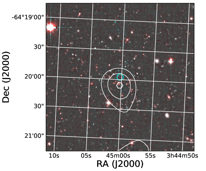
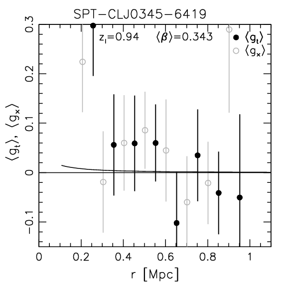
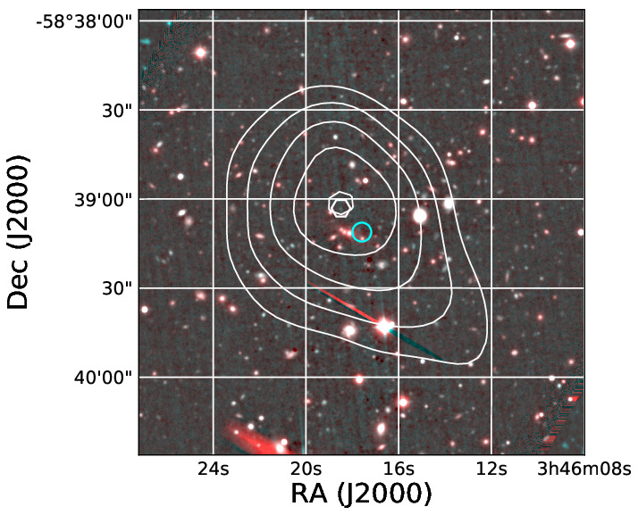
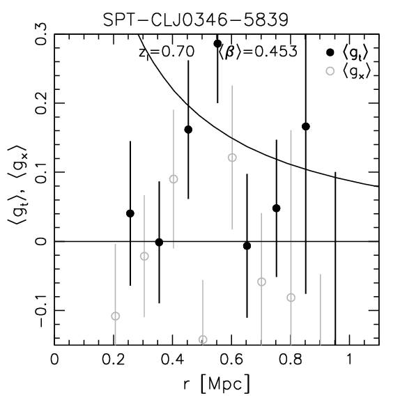
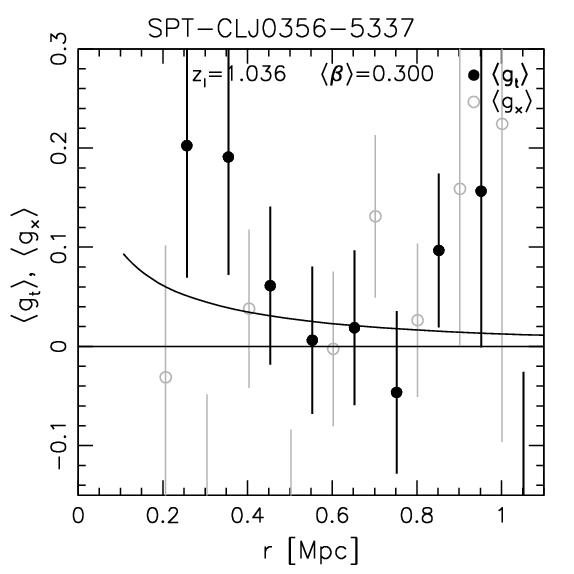
Figure 17: WL results for clusters from the ACS+GMOS sample (continued, see Fig. 15 for details).

Among the clusters in the ACS+GMOS sample, we obtain detections with $S/N_{\mathrm{peak}}\geq 3$ for SPT-CL $J$0058$-$6145, SPT-CL $J$0258$-$5355, SPT-CL $J$0346$-$5839, SPT-CL $J$0422$-$4608, SPT-CL $J$0444$-$5603, SPT-CL $J$0516$-$5755, SPT-CL $J$0530$-$4139, and SPT-CL $J$0540$-$5744 (see Table 6), as well as tentative detections ($S/N_{\mathrm{peak}}\geq 2$) for SPT-CL $J$0339$-$4545, SPT-CL $J$0345$-$6419, SPT-CL $J$0617$-$5507, SPT-CL $J$2228$-$5828 and SPT-CL $J$2311$-$5820⁸. Furthermore, SPT-CL $J$0356$-$5337, which is a potential dissociative merger based on strong lensing features (Mahler et al., 2020), shows a weak peak ($S/N_{\mathrm{peak}}=1.6$, see the bottom-left panel of Fig. 17) close to the BCG candidate from Mahler et al. (2020). We suspect that the main reasons for the poorer detection rate in the WL mass reconstructions of the ACS+GMOS sample are given by the smaller field covered by these observations and the (on average) expected lower masses of the clusters.

4.2 NFW fits to reduced shear profiles

Table 7: Weak lensing mass constraints from the NFW fits to the reduced shear profiles around the X-ray centres for the clusters with ACS mosaics for two different over-densities $\Delta\in\{200\mathrm{c},500\mathrm{c}\}$. The top (bottom) set of rows corresponds to clusters with (without) new observations. $M_{\Delta}^{\mathrm{biased,ML}}$ are maximum likelihood mass estimates in $10^{14}\mathrm{M}_{\odot}$ without corrections for mass modelling bias applied. The listed errors are statistical 68% uncertainties, including the contributions from shape noise (asymmetric errors), uncorrelated large-scale, and line-of-sight variations in the redshift distribution. Systematic uncertainties are listed in Table 11. $\hat{b}_{\mathrm{\Delta,WL}}=\text{exp}\left[\langle\text{ln}\,b_{\Delta,\text{WL}}\rangle\right]$ relates to the mean of the estimated mass bias distribution, whose width is characterised by $\sigma(\mathrm{ln}\,b_{\mathrm{\Delta,WL}})$.

Cluster	$M_{200\mathrm{c}}^{\mathrm{biased,ML}}\,[10^{14}\mathrm{M}_{\odot}]$	$\hat{b}_{200\mathrm{c,WL}}$	$\sigma(\mathrm{ln}\,b_{\mathrm{\mathrm{200c,WL}}})$	$M_{500\mathrm{c}}^{\mathrm{biased,ML}}\,[10^{14}\mathrm{M}_{\odot}]$	$\hat{b}_{500\mathrm{c,WL}}$	$\sigma(\mathrm{ln}\,b_{\mathrm{\mathrm{500c,WL}}})$
SPT-CL $J$0000$-$5748	$6.0_{-2.2}^{+2.4}\pm 1.1\pm 0.3$	$0.89\pm 0.01$	$0.35\pm 0.01$	$4.1_{-1.5}^{+1.7}\pm 0.8\pm 0.2$	$0.91\pm 0.01$	$0.32\pm 0.01$
SPT-CL $J$0533$-$5005	$4.0_{-2.0}^{+2.3}\pm 1.0\pm 0.2$	$0.91\pm 0.02$	$0.32\pm 0.02$	$2.7_{-1.4}^{+1.6}\pm 0.7\pm 0.2$	$0.91\pm 0.01$	$0.28\pm 0.02$
SPT-CL $J$2040$-$5726	$3.5_{-2.1}^{+2.6}\pm 0.9\pm 0.2$	$0.91\pm 0.02$	$0.32\pm 0.02$	$2.4_{-1.5}^{+1.8}\pm 0.6\pm 0.2$	$0.90\pm 0.01$	$0.26\pm 0.03$
SPT-CL $J$2043$-$5035	$4.3_{-1.9}^{+2.1}\pm 0.9\pm 0.3$	$0.92\pm 0.01$	$0.32\pm 0.01$	$2.9_{-1.3}^{+1.5}\pm 0.7\pm 0.2$	$0.93\pm 0.01$	$0.28\pm 0.02$
SPT-CL $J$2337$-$5942	$10.9_{-2.6}^{+2.6}\pm 1.3\pm 0.6$	$0.88\pm 0.02$	$0.37\pm 0.02$	$7.6_{-1.8}^{+1.9}\pm 0.9\pm 0.4$	$0.89\pm 0.01$	$0.33\pm 0.02$
SPT-CL $J$2341$-$5119	$3.5_{-2.1}^{+2.5}\pm 1.1\pm 0.2$	$0.90\pm 0.01$	$0.31\pm 0.01$	$2.4_{-1.5}^{+1.8}\pm 0.8\pm 0.2$	$0.89\pm 0.01$	$0.30\pm 0.01$
SPT-CL $J$2359$-$5009	$6.2_{-2.3}^{+2.5}\pm 1.1\pm 0.3$	$0.92\pm 0.01$	$0.31\pm 0.02$	$4.3_{-1.6}^{+1.8}\pm 0.8\pm 0.2$	$0.93\pm 0.01$	$0.26\pm 0.03$
SPT-CL $J$0102$-$4915	$11.9_{-2.9}^{+3.0}\pm 1.2\pm 0.9$	$0.87\pm 0.06$	$0.37\pm 0.05$	$8.6_{-2.2}^{+2.2}\pm 0.9\pm 0.6$	$0.84\pm 0.02$	$0.38\pm 0.02$
SPT-CL $J$0546$-$5345	$5.1_{-3.2}^{+3.7}\pm 1.1\pm 0.5$	$0.84\pm 0.02$	$0.37\pm 0.02$	$3.5_{-2.2}^{+2.7}\pm 0.8\pm 0.3$	$0.85\pm 0.02$	$0.35\pm 0.02$
SPT-CL $J$0559$-$5249	$8.1_{-3.0}^{+3.2}\pm 1.1\pm 0.5$	$0.84\pm 0.01$	$0.42\pm 0.02$	$5.5_{-2.1}^{+2.3}\pm 0.7\pm 0.4$	$0.86\pm 0.01$	$0.39\pm 0.01$
SPT-CL $J$0615$-$5746	$8.1_{-2.7}^{+2.9}\pm 1.2\pm 0.7$	$0.84\pm 0.02$	$0.34\pm 0.02$	$5.6_{-1.9}^{+2.1}\pm 0.9\pm 0.5$	$0.85\pm 0.02$	$0.32\pm 0.02$
SPT-CL $J$2106$-$5844	$8.4_{-4.5}^{+5.0}\pm 1.5\pm 0.9$	$0.80\pm 0.03$	$0.43\pm 0.04$	$5.9_{-3.3}^{+3.7}\pm 1.1\pm 0.6$	$0.80\pm 0.03$	$0.40\pm 0.04$
SPT-CL $J$2331$-$5051	$4.8_{-2.3}^{+2.7}\pm 1.0\pm 0.3$	$0.86\pm 0.01$	$0.39\pm 0.01$	$3.3_{-1.6}^{+1.9}\pm 0.7\pm 0.2$	$0.89\pm 0.01$	$0.35\pm 0.01$
SPT-CL $J$2342$-$5411	$8.8_{-3.7}^{+4.0}\pm 1.3\pm 0.9$	$0.87\pm 0.02$	$0.37\pm 0.02$	$6.2_{-2.6}^{+2.9}\pm 0.9\pm 0.6$	$0.88\pm 0.02$	$0.38\pm 0.03$

Table 8: As Table 7, but for the analysis centring on the SZ peak locations.

Cluster	$M_{200\mathrm{c}}^{\mathrm{biased,ML}}\,[10^{14}\mathrm{M}_{\odot}]$	$\hat{b}_{200\mathrm{c,WL}}$	$\sigma(\mathrm{ln}\,b_{\mathrm{\mathrm{200c,WL}}})$	$M_{500\mathrm{c}}^{\mathrm{biased,ML}}\,[10^{14}\mathrm{M}_{\odot}]$	$\hat{b}_{500\mathrm{c,WL}}$	$\sigma(\mathrm{ln}\,b_{\mathrm{\mathrm{500c,WL}}})$
SPT-CL $J$0000$-$5748	$6.5_{-2.2}^{+2.4}\pm 1.1\pm 0.3$	$0.85\pm 0.01$	$0.32\pm 0.01$	$4.4_{-1.5}^{+1.7}\pm 0.8\pm 0.2$	$0.86\pm 0.01$	$0.29\pm 0.01$
SPT-CL $J$0533$-$5005	$2.0_{-1.5}^{+2.0}\pm 0.8\pm 0.1$	$0.87\pm 0.01$	$0.31\pm 0.01$	$1.3_{-1.0}^{+1.4}\pm 0.5\pm 0.1$	$0.85\pm 0.01$	$0.29\pm 0.01$
SPT-CL $J$2040$-$5726	$4.3_{-2.3}^{+2.7}\pm 1.0\pm 0.3$	$0.84\pm 0.02$	$0.30\pm 0.03$	$2.9_{-1.6}^{+1.9}\pm 0.7\pm 0.2$	$0.81\pm 0.02$	$0.31\pm 0.03$
SPT-CL $J$2043$-$5035	$3.6_{-1.8}^{+2.1}\pm 1.0\pm 0.3$	$0.87\pm 0.01$	$0.31\pm 0.01$	$2.4_{-1.2}^{+1.4}\pm 0.7\pm 0.2$	$0.89\pm 0.01$	$0.29\pm 0.01$
SPT-CL $J$2337$-$5942	$10.7_{-2.6}^{+2.6}\pm 1.3\pm 0.6$	$0.86\pm 0.01$	$0.32\pm 0.02$	$7.5_{-1.8}^{+1.9}\pm 0.9\pm 0.4$	$0.87\pm 0.01$	$0.28\pm 0.01$
SPT-CL $J$2341$-$5119	$3.2_{-2.1}^{+2.5}\pm 1.0\pm 0.2$	$0.83\pm 0.02$	$0.32\pm 0.02$	$2.2_{-1.4}^{+1.7}\pm 0.7\pm 0.2$	$0.83\pm 0.01$	$0.29\pm 0.01$
SPT-CL $J$2359$-$5009	$5.4_{-2.2}^{+2.4}\pm 1.1\pm 0.3$	$0.87\pm 0.01$	$0.30\pm 0.02$	$3.7_{-1.5}^{+1.7}\pm 0.8\pm 0.2$	$0.87\pm 0.01$	$0.26\pm 0.02$
SPT-CL $J$0102$-$4915	$15.2_{-2.8}^{+2.8}\pm 1.1\pm 1.1$	$0.77\pm 0.05$	$0.37\pm 0.06$	$11.1_{-2.1}^{+2.2}\pm 0.8\pm 0.8$	$0.79\pm 0.02$	$0.33\pm 0.03$
SPT-CL $J$0546$-$5345	$2.5_{-2.3}^{+3.5}\pm 1.0\pm 0.2$	$0.75\pm 0.02$	$0.37\pm 0.02$	$1.7_{-1.6}^{+2.4}\pm 0.7\pm 0.2$	$0.75\pm 0.01$	$0.34\pm 0.03$
SPT-CL $J$0559$-$5249	$4.2_{-2.4}^{+2.9}\pm 0.9\pm 0.3$	$0.79\pm 0.01$	$0.39\pm 0.02$	$2.8_{-1.6}^{+2.0}\pm 0.6\pm 0.2$	$0.83\pm 0.01$	$0.36\pm 0.01$
SPT-CL $J$0615$-$5746	$7.1_{-2.6}^{+2.8}\pm 1.2\pm 0.6$	$0.84\pm 0.02$	$0.27\pm 0.03$	$4.9_{-1.8}^{+2.1}\pm 0.8\pm 0.4$	$0.84\pm 0.01$	$0.25\pm 0.02$
SPT-CL $J$2106$-$5844	$8.2_{-4.4}^{+4.9}\pm 1.4\pm 0.8$	$0.73\pm 0.03$	$0.38\pm 0.05$	$5.7_{-3.2}^{+3.7}\pm 1.0\pm 0.6$	$0.77\pm 0.03$	$0.29\pm 0.07$
SPT-CL $J$2331$-$5051	$5.2_{-2.4}^{+2.7}\pm 1.0\pm 0.3$	$0.86\pm 0.01$	$0.34\pm 0.01$	$3.5_{-1.6}^{+1.9}\pm 0.7\pm 0.2$	$0.88\pm 0.01$	$0.30\pm 0.01$
SPT-CL $J$2342$-$5411	$7.4_{-3.5}^{+3.9}\pm 1.1\pm 0.7$	$0.80\pm 0.02$	$0.38\pm 0.03$	$5.1_{-2.5}^{+2.8}\pm 0.8\pm 0.5$	$0.81\pm 0.02$	$0.33\pm 0.04$

In order to constrain the cluster masses we estimate the binned profiles of the tangential component of the reduced shear $g$ with respect to the corresponding cluster centre

$$g_{\mathrm{t}}=-g_{1}\cos{2\phi}-g_{2}\sin{2\phi}\,,$$ (9)

where $\phi$ indicates the azimuthal angle with respect to the centre. Here, the reduced shear $g=g_{1}+\mathrm{i}g_{2}$ is written in terms of its component along the coordinate grid $g_{1}$ and the 45deg-rotated component $g_{2}$. Following S18 we estimate the reduced shear profile $\langle g_{\mathrm{t}}\rangle(r_{k},V_{j})=\sum(w_{i}\epsilon_{\mathrm{t},i})/\sum w_{i}$ for each cluster in bins of radius $r_{k}$ and magnitude $V_{j}$, where $w_{i}$ indicates the shape weight and the sum is computed over all galaxies $i$ falling into the corresponding radius and magnitude bin combination. Accounting for the magnitude dependence increases the sensitivity of the analysis given the dependence of $\langle\beta\rangle$ on $V_{606}$ (see Fig. 4). For each cluster we then jointly fit the $\langle g_{\mathrm{t}}\rangle(r_{k},V_{j})$ profiles with predictions for spherical NFW (Navarro, Frenk & White, 1997) density profiles according to Wright & Brainerd (2000), assuming the concentration–mass ($c(M)$) relation from Diemer & Joyce (2019). When computing model predictions we also correct for the impact of weak lensing magnification on $\langle\beta\rangle$ following S18, as well as the finite width of the redshift distribution following Seitz & Schneider (1997); Hoekstra, Franx & Kuijken (2000) and Applegate et al. (2014). For the clusters with ACS mosaics we compute shear profiles both around the SZ peak locations and the X-ray centroids (see Table 1). Since high-resolution X-ray observations are presently unavailable for most clusters in the ACS+GMOS sample, we employ the SZ peak locations as centres when computing shear profiles for these clusters. Both centre proxies typically deviate from the location of the halo centre, which would be used in simulation analyses to define over-density cluster masses. We describe in Sect. 4.3 how we account for the mass modelling bias that results from this and other effects, but to limit their impact we only include scale $r>500$kpc in the fit, as done by S18. Following them we also limit the fit to scales $r<1.5$Mpc for the clusters with ACS mosaics. The right panels of Figs. 12 to 20 show the resulting reduced tangential shear profiles (scaled to the average $\langle\beta\rangle$ and combined as done by S18), best-fit NFW models, and profiles of the 45deg-rotated reduced shear cross component

$$g_{\times}=g_{1}\sin{2\phi}-g_{2}\cos{2\phi}\,,$$ (10)

which should be consistent with zero in the absence of PSF-related systematics.

We list the constraints on the best-fitting mass within a sphere that has an average density of 200 times the critical density of the Universe at the cluster redshift ($M_{\mathrm{200c}}$) and the corresponding $M_{\mathrm{500c}}$ estimates (assuming the $c(M)$ relation from Diemer & Joyce, 2019) in Tables 7, 8, and 9. There we not only list the statistical uncertainties from the NFW shear profile fit and shape noise, but also contributions from uncorrelated large-scale structure projections (computed using Gaussian cosmic shear field realisations following Simon, 2012, see also S18) and line-of-sight variations in the source redshift distribution (see Sect. 3.4). For the clusters in the ACS+GMOS sample (see Table 2) we also list the mass uncertainty resulting from the photometric cluster redshift uncertainties. Note that the maximum likelihood mass estimates reported in Tables 7 to 9 have not yet been corrected for mass modelling biases. Our procedure to correct for these biases is described in Sect. 4.3 and applied in the scaling relation analysis is Sect. 5.

Comparing entries in Tables 7 and 8 versus Table 9 it is evident that the observations using $2\times 2$ ACS mosaics yield much tighter mass constraints given their better radial coverage. E.g., comparing the results for SPT-CL J2337$-$5942 and SPT-CL J0530$-$4139, which have similar cluster redshifts and best-fit WL mass estimates, we find that the relative statistical mass errors are larger by a factor 1.8 for the single-pointing ACS data. We expect that these large fit uncertainties, together with a larger intrinsic scatter (see Sect. 4.3) are primarily responsible for the large spread in best-fitting mass estimates reported in Table 9 for the ACS+GMOS sample, for which we would expect a relatively low scatter in halo mass based on their SZ signature (Table 2).

Table 9: Weak lensing mass constraints from the NFW fits to the reduced shear profiles around the SZ peaks of the clusters in the ACS+GMOS sample for two different over-densities $\Delta\in\{200\mathrm{c},500\mathrm{c}\}$. $M_{\Delta}^{\mathrm{biased,ML}}$ are maximum likelihood mass estimates in $10^{14}\mathrm{M}_{\odot}$ without corrections for mass modelling bias applied. The listed errors are statistical 68% uncertainties, including the contributions from shape noise (asymmetric errors), uncorrelated large-scale, line-of-sight variations in the redshift distribution, and the uncertainty in the (photometric) cluster redshift. Systematic uncertainties are listed in Table 11. $\hat{b}_{\mathrm{\Delta,WL}}=\text{exp}\left[\langle\text{ln}\,b_{\Delta,\text{WL}}\rangle\right]$ relates to the mean of the estimated mass bias distribution, whose width is characterised by $\sigma(\mathrm{ln}\,b_{\mathrm{\Delta,WL}})$.

Cluster	$M_{200\mathrm{c}}^{\mathrm{biased,ML}}\,[10^{14}\mathrm{M}_{\odot}]$	$\hat{b}_{200\mathrm{c,WL}}$	$\sigma(\mathrm{ln}\,b_{\mathrm{\mathrm{200c,WL}}})$	$M_{500\mathrm{c}}^{\mathrm{biased,ML}}\,[10^{14}\mathrm{M}_{\odot}]$	$\hat{b}_{500\mathrm{c,WL}}$	$\sigma(\mathrm{ln}\,b_{\mathrm{\mathrm{500c,WL}}})$
SPT-CL $J$0044$-$4037	$-0.2_{-2.9}^{+2.1}\pm 0.3\pm 0.0\pm 0.4$	$0.76\pm 0.05$	$0.40\pm 0.08$	$-0.1_{-2.0}^{+1.4}\pm 0.2\pm 0.0\pm 0.2$	$0.74\pm 0.03$	$0.39\pm 0.06$
SPT-CL $J$0058$-$6145	$7.7_{-4.1}^{+4.4}\pm 0.9\pm 0.8\pm 0.8$	$0.76\pm 0.02$	$0.41\pm 0.03$	$5.3_{-2.9}^{+3.2}\pm 0.6\pm 0.6\pm 0.5$	$0.78\pm 0.02$	$0.33\pm 0.04$
SPT-CL $J$0258$-$5355	$13.9_{-4.5}^{+4.2}\pm 1.0\pm 1.5\pm 1.9$	$0.64\pm 0.04$	$0.53\pm 0.08$	$10.1_{-3.4}^{+3.2}\pm 0.8\pm 1.1\pm 1.6$	$0.68\pm 0.04$	$0.39\pm 0.07$
SPT-CL $J$0339$-$4545	$2.5_{-2.5}^{+4.0}\pm 0.7\pm 0.3\pm 0.5$	$0.75\pm 0.04$	$0.43\pm 0.06$	$1.7_{-1.7}^{+2.8}\pm 0.5\pm 0.2\pm 0.4$	$0.73\pm 0.03$	$0.46\pm 0.05$
SPT-CL $J$0344$-$5452	$6.8_{-5.4}^{+6.2}\pm 1.1\pm 0.7\pm 1.7$	$0.71\pm 0.03$	$0.44\pm 0.05$	$4.8_{-3.8}^{+4.6}\pm 0.8\pm 0.5\pm 1.2$	$0.68\pm 0.03$	$0.49\pm 0.06$
SPT-CL $J$0345$-$6419	$0.0_{-3.0}^{+2.9}\pm 0.3\pm 0.0\pm 0.2$	$0.79\pm 0.04$	$0.40\pm 0.08$	$0.0_{-2.1}^{+1.9}\pm 0.2\pm 0.0\pm 0.1$	$0.80\pm 0.03$	$0.32\pm 0.06$
SPT-CL $J$0346$-$5839	$12.2_{-6.0}^{+6.0}\pm 1.0\pm 1.2\pm 1.5$	$0.78\pm 0.05$	$0.41\pm 0.10$	$8.5_{-4.2}^{+4.3}\pm 0.7\pm 0.8\pm 1.1$	$0.80\pm 0.05$	$0.36\pm 0.07$
SPT-CL $J$0356$-$5337	$1.1_{-2.2}^{+4.0}\pm 0.7\pm 0.1\pm 0.0$	$0.76\pm 0.03$	$0.42\pm 0.06$	$0.8_{-1.5}^{+2.8}\pm 0.5\pm 0.1\pm 0.0$	$0.77\pm 0.03$	$0.35\pm 0.05$
SPT-CL $J$0422$-$4608	$9.8_{-6.1}^{+6.6}\pm 1.0\pm 0.8\pm 1.6$	$0.73\pm 0.05$	$0.46\pm 0.09$	$6.7_{-4.3}^{+4.7}\pm 0.7\pm 0.6\pm 1.1$	$0.79\pm 0.04$	$0.39\pm 0.09$
SPT-CL $J$0444$-$5603	$7.4_{-4.4}^{+4.8}\pm 0.9\pm 0.8\pm 0.6$	$0.76\pm 0.04$	$0.41\pm 0.09$	$5.1_{-3.1}^{+3.4}\pm 0.7\pm 0.5\pm 0.3$	$0.76\pm 0.04$	$0.41\pm 0.06$
SPT-CL $J$0516$-$5755	$2.8_{-3.2}^{+5.3}\pm 0.9\pm 0.3\pm 0.1$	$0.77\pm 0.05$	$0.37\pm 0.10$	$1.9_{-2.2}^{+3.8}\pm 0.6\pm 0.2\pm 0.1$	$0.78\pm 0.04$	$0.32\pm 0.06$
SPT-CL $J$0530$-$4139	$8.8_{-4.5}^{+4.6}\pm 0.9\pm 0.9\pm 0.7$	$0.76\pm 0.02$	$0.42\pm 0.04$	$6.1_{-3.1}^{+3.3}\pm 0.7\pm 0.6\pm 0.5$	$0.78\pm 0.02$	$0.39\pm 0.04$
SPT-CL $J$0540$-$5744	$8.4_{-4.3}^{+4.7}\pm 0.9\pm 0.8\pm 0.0$	$0.79\pm 0.02$	$0.40\pm 0.04$	$5.8_{-3.0}^{+3.4}\pm 0.7\pm 0.5\pm 0.0$	$0.81\pm 0.03$	$0.39\pm 0.03$
SPT-CL $J$0617$-$5507	$1.3_{-2.3}^{+4.1}\pm 0.6\pm 0.2\pm 0.6$	$0.75\pm 0.04$	$0.41\pm 0.07$	$0.9_{-1.5}^{+2.9}\pm 0.4\pm 0.1\pm 0.4$	$0.72\pm 0.03$	$0.40\pm 0.06$
SPT-CL $J$2228$-$5828	$2.4_{-2.4}^{+3.7}\pm 0.7\pm 0.2\pm 0.4$	$0.64\pm 0.03$	$0.54\pm 0.06$	$1.6_{-1.6}^{+2.6}\pm 0.5\pm 0.1\pm 0.3$	$0.64\pm 0.03$	$0.47\pm 0.05$
SPT-CL $J$2311$-$5820	$9.5_{-4.8}^{+5.0}\pm 0.9\pm 0.9\pm 0.8$	$0.78\pm 0.04$	$0.41\pm 0.07$	$6.6_{-3.4}^{+3.7}\pm 0.7\pm 0.7\pm 0.6$	$0.74\pm 0.03$	$0.37\pm 0.06$

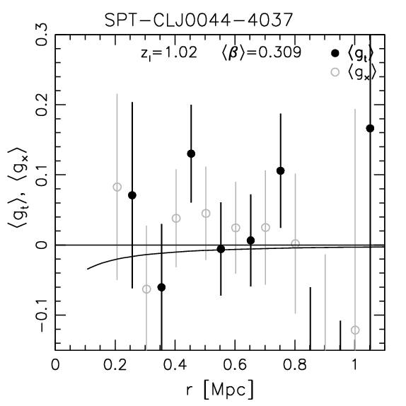
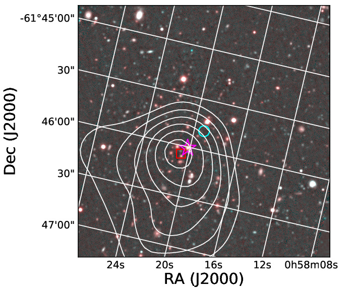
Figure 15: WL results for clusters from the ACS+GMOS sample. Left: Signal-to-noise ratio map of the WL mass reconstruction (starting at $1.5\sigma$ in steps of $0.5\sigma$, with the peak indicated by the hexagon), overlaid on a colour image using the PSF-homogenised ACS/F606W image for the blue and green channels, and the GMOS $i$-band image for the red channel ($2\aas@@fstack{\prime}5\times 2\aas@@fstack{\prime}5$ cutout). Differing from Figs. 12 to 14 we show the extra contour at $1.5\sigma$ since the mass reconstructions are more strongly affected by the mass-sheet degeneracy for the ACS+GMOS sample (see Sect. 4.1), leading to a stronger underestimation of the true $S/N$. The SZ peak is shown by the cyan circle. For SPT-CL $J$0058$-$6145 we additionally mark the X-ray centre from McDonald et al. (2013, red square) and the BCG candidate from Zenteno et al. (2020, magenta star). Right: Combined reduced shear profile around the SZ centre, showing the tangential (black solid circles with best-fitting NFW model) and cross (grey open circles, shifted along the $x$-axis for clarity) components.

Note. — Because of noise (from the intrinsic galaxy shapes and large-scale structure projections) the tangential reduced shear profiles of individual clusters may become slightly negative on average, as is the case for SPT-CL $J$0044$-$4037 (see Fig. 15). For the mass limits reported in this table we model such negative profiles by allowing for (unphysical) negative cluster masses. Here we employ the NFW reduced shear profile prediction of the corresponding positive mass, but switch the sign of the model.

4.3 Correction for mass modelling biases

Systematic deviations from the NFW model, uncertainties and scatter in the assumed $c(M)$ relation (e.g. Child et al., 2018), triaxiality, correlated large-scale structure, and miscentring of the fitted profile can lead to systematic biases in the measured masses. Here we describe our method of constraining the distribution of the net bias, excluding contributions from uncorrelated large-scale structure (the latter effect is discussed in Sect. 4.2). Following Becker & Kravtsov (2011), we define the bias for an individual target through

$$M_{\Delta,\text{WL}}=b_{\Delta,\text{WL}}M_{\Delta,\text{halo}},$$ (11)

where $M_{\Delta,\text{WL}}$ is the mass at overdensity $\Delta$ measured from the reduced shear profile, $M_{\Delta,\text{halo}}$ is the corresponding halo mass and $b_{\Delta,\text{WL}}$ is the bias factor.

We use simulations to estimate the bias distribution for each of our targets, including a mass dependence. In particular, following S18 and D19 we use the $z=0.25$ and $z=1.0$ snapshots of the Millennium-XXL simulations (Angulo et al., 2012), from which reduced shear fields of massive halos are derived, using the lensing efficiencies of the individual targets. After choosing a centre that either corresponds to the 3D halo centre or a miscentred position (explained below), we bin the tangential reduced shear profile, to which we add shape noise that matches the uncertainties of the actual cluster tangential reduced shear estimates in each corresponding radial bin. We then fit the cluster masses from the noisy mock data as done for the real cluster observations. Halo-related properties, such as the lens redshift, are scaled appropriately, while cosmology-related properties, such as the redshift dependence in the mass-concentration relation, are kept at the redshifts of the simulation in the respective snapshots.

In the presence of noise, it is difficult to model the bias distribution generally. Following recent work including S18, D19, and B19 we therefore make the simplifying assumption of a log-normal (in halo mass) distribution. The distribution is defined by the expectation value $\mu$ and the dispersion $\sigma$ in the natural-log space of $b_{\Delta,\text{WL}}$, such that $\mu=\langle\text{ln}\,b_{\Delta,\text{WL}}\rangle$ and $\sigma^{2}$ is the variance of $\text{ln}\,b_{\Delta,\rm{WL}}$. We further define

$$\hat{b}_{\Delta,\text{WL}}=\text{exp}\left[\langle\text{ln}\,b_{\Delta,\text{WL}}\rangle\right]\,$$ (12)

as a measure of the bias in linear space (with the caveat that this measure alone cannot be used in order to remove the mass bias). The Bayesian framework for this analysis was already summarised in S18 and D19. It closely matches the approach employed in Lee et al. (2018), to which we refer the reader for a more detailed description. For each target, mass bin, overdensity ($500c$ and $200c$) and simulation snapshot, we derive the mean and scatter of the log-normal, and interpolate linearly between the snapshots to the redshift of the target. We note that for any mass bin, the bias amplitudes inferred from the two simulation snapshots differ by at most $10\%$.

As a prior on the mass, we use the SZ-derived masses ($M_{500c,\text{SZ}}$ and $M_{200c,\text{SZ}}$) from B19. We use the asymmetric distributions of these mass priors to marginalise over the mass dependence of the weak-lensing bias, to arrive at a final mean and dispersion for each target.

To additionally account for miscentring, we add a step to the procedure described above. Prior to fitting masses, we offset the shear field on the sky in a random direction, where the magnitude of the offset is drawn from a miscentring distribution. In this paper, we use the two miscentring distributions also used by S18, derived from the Magneticum Pathfinder Simulation (Dolag, Komatsu & Sunyaev, 2016) and based on using X-ray centroids and SZ peaks from the simulation as proxies (see Appendix C for details). A shortcoming of this approach is that all clusters, mergers and relaxed systems alike, are treated in the same way, while we would expect the miscentring to be greater, on average, in merging systems (e.g. Bleem et al., 2020; Zenteno et al., 2020). In a future work (Sommer et al., in prep.), we plan to use hydrodynamical simulations to explore the bias magnitude due to miscentring for different dynamical states.

We list the estimates for $\hat{b}_{\Delta,\text{WL}}$ and the scatter $\sigma(\mathrm{ln}\,b_{\mathrm{\Delta,\text{WL}}})$ including their statistical uncertainties for the different clusters incorporating miscentring in Tables 7, 8 and 9. For clusters already studied in S18, slight to moderate shifts can occur in the reported bias values for two reasons: First, we now account for a mass dependence of the bias (see also Sommer et al., 2021). Second, our modifications in the source selection (especially for the clusters with new VLT data) changes the relative contributions of scales at different radii, thereby affecting the mass modelling bias.

The average bias values are summarised in Table 10, showing that masses are expected to be biased by $-5\%$ to $-6\%$ when centred on the 3D halo centre. Miscentring increases the bias by $-7\%$ for ACS mosaics and X-ray centres, $-12\%$ in the case of ACS mosaics and SZ centres, and $-19\%$ for the ACS+GMOS observations and SZ centres, which are more strongly affected because of the smaller field of view. Comparing Tables 8 and 9 we see that the limited radial coverage provided by the ACS+GMOS observations also leads to a substantial increase in the estimated intrinsic scatter $\sigma(\mathrm{ln}\,b_{\mathrm{\mathrm{500c,WL}}})$.

The largest systematic uncertainty related to these bias estimates is given by the uncertainty in the miscentring correction. As a conservative estimate S18 assume that this uncertainty would at most be half of the actual correction. Here we follow their conservative assumption, not only because of uncertainties in the assumed miscentring distributions, but also because our simulation analysis suggests that the assumption of a log-normal scatter is not strictly met when miscentring is included (see Sommer et al., 2021). This constitutes the largest contribution to our systematic error budget for the analysis using SZ centres (see Sect. 4.4), highlighting the importance of reducing this uncertainty in future WL studies of larger samples.

As a cross-check for the miscentring correction we compare the WL mass estimates obtained for the clusters with ACS mosaics using the X-ray centres versus using the SZ centres in Fig. 6, applying approximate corrections for the corresponding mass modelling biases. The median ratio $1.05\pm 0.09$ of the corrected estimates is consistent with unity, as one would expect in case of an accurate correction. Given the limited sample size the statistical uncertainty of this ratio (estimated by bootstrapping the clusters) is still substantial, exceeding the estimated systematic uncertainty of the miscentring correction (compare Table 11). Future studies using larger samples should, however, be able to use similar cross-checks to test their miscentring corrections at a useful precision.

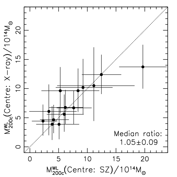
Figure 6: Comparison of the best-fitting WL mass estimates obtained for the clusters with ACS mosaics using the X-ray centres versus the SZ centres, approximately corrected for mass modelling bias as $M_{200\mathrm{c}}^{\mathrm{WL}}=M_{200\mathrm{c}}^{\mathrm{biased,ML}}/\hat{b}_{200\mathrm{c,WL}}$. The error-bars correspond to the combined statistical errors given in Tables 7 and 8, respectively, but do not include the additional scatter inferred from the simulations.

An additional source of systematic uncertainty is given by the impact of baryons, which may systematically shift the distributions of cluster concentrations compared to the N-body simulations we are using to calibrate mass modelling biases. S18 estimate that this could lead to a mass bias uncertainty of 2–4%, where we conservatively assume a 4% uncertainty in our systematic error budget.

Table 10: Simulation-derived estimates of $\hat{b}_{\mathrm{\Delta,WL}}$ for different miscentring distributions and overdensities, averaged over different cluster samples. The individual bias estimates and their statistical errors are listed in Tables 7, 8 and 9.

Miscentring	Setup	$\langle\hat{b}_{\mathrm{200c,WL}}\rangle$	$\langle\hat{b}_{\mathrm{500c,WL}}\rangle$
None	ACS mosaics	0.95	0.95
None	ACS+GMOS	0.94	0.95
X-ray	ACS mosaics	0.87	0.88
X-ray	ACS+GMOS	0.83	0.83
SZ	ACS mosaics	0.82	0.83
SZ	ACS+GMOS	0.75	0.75

4.4 Systematic error summary

We summarise the systematic error contributions described in Sections 3.1, 3.4, and 4.3 in Table 11. For the clusters with ACS mosaics the total systematic uncertainty amounts to 7.5% when using X-ray centres and 9.0% for SZ centres. The systematic uncertainty increases to 11.6% for the analysis using SZ centres and ACS+GMOS observations due to their smaller field of view.

Table 11: Systematic error budget for our current study.

Source	rel. error	rel. error $M_{\mathrm{500c}}$
	signal
Shape measurements:
Shear calibration	1.5%	2.3%
Redshift distribution:
Photo-$z$ sys. + sampling variance	3.0%	4.5%
Deblending	0.5%	0.8%
Blue member contamination	0.9%	1.4%
Mass model:
$c(M)$ relation		4%
Miscentring for
ACS mosaics + X-ray centres		3.5%
/ ACS mosaics + SZ centres		6%
/ ACS+GMOS + SZ centres		9.5%
Total:		7.5% / 9.0% / 11.6%

5 Constraints on the SPT observable–mass relation

We use the extended and updated HST WL data-set (HST-30) to constrain the SPT observable–mass relation. As in other recent SPT work, we also use the set of 19 weak-lensing observations of SPT clusters from Magellan/Megacam presented in D19 (Megacam-19). Our full sample of SPT clusters with WL data then contains 49 objects. In some comparisons conducted below we alternatively employ the previous HST weak lensing data set of 13 clusters (HST-13) from S18 (not applying our updated calibrations and source selections).

5.1 Observable–mass relation model and likelihood function

Following previous SPT work (e.g., Vanderlinde et al., 2010), we describe the unbiased detection significance $\zeta$ as a power law in mass and the dimensionless Hubble parameter $E(z)\equiv H(z)/H_{0}$

$$\langle\ln\zeta\rangle=\ln\left[\gamma_{\mathrm{field}}{A_{\mathrm{SZ}}}\left(\frac{M_{500c}}{3\times 10^{14}\mathrm{M}_{\odot}/h}\right)^{B_{\mathrm{SZ}}}\left(\frac{E(z)}{E(0.6)}\right)^{C_{\mathrm{SZ}}}\right],$$ (13)

where ${A_{\mathrm{SZ}}}$, ${B_{\mathrm{SZ}}}$, and ${C_{\mathrm{SZ}}}$ are the scaling relation parameters and $\gamma_{\mathrm{field}}$ describes the effective depth of each of the SPT fields (e.g., de Haan et al., 2016). The unbiased significance $\zeta$ is related to the detection significance $\xi$ via

$$P(\xi|\zeta)=\mathcal{N}(\sqrt{\zeta^{2}+3},1).$$ (14)

The relationship between the lensing mass $M_{\mathrm{WL}}$ and the halo mass was defined earlier in Eq. 11 (in the current section we always use $\Delta=500\mathrm{c}$ and therefore suppress this index for better readability). The following covariance matrix describes the correlated intrinsic scatter between the logarithms of the two observables $\zeta$ and $M_{\mathrm{WL}}$

$$\mathbf{\Sigma}_{\zeta-M_{\mathrm{WL}}}=\begin{pmatrix}\sigma_{\ln\zeta}^{2}&\rho_{\mathrm{SZ}-\mathrm{WL}}\sigma_{\ln\zeta}\sigma_{\ln M_{\mathrm{WL}}}\\ \rho_{\mathrm{SZ}-\mathrm{WL}}\sigma_{\ln\zeta}\sigma_{\ln M_{\mathrm{WL}}}&\sigma_{\ln M_{\mathrm{WL}}}^{2}\end{pmatrix}.$$ (15)

The joint scaling relation then reads

$$P\Bigl{(}\begin{bmatrix}\ln\zeta\\ \ln M_{\mathrm{WL}}\end{bmatrix}|M,z\Bigr{)}=\mathcal{N}\Bigl{(}\begin{bmatrix}\langle\ln\zeta\rangle(M,z)\\ \langle\ln M_{\mathrm{WL}}\rangle(M,z)\end{bmatrix},\mathbf{\Sigma}_{\zeta-M_{\mathrm{WL}}}\Bigr{)}.$$ (16)

Following previous work (D19, B19), we compute the likelihood function for each cluster with weak-lensing data as

$$\begin{split}P(g_{\mathrm{t}}|\xi,z,\boldsymbol{p})=\iiint&\mathrm{d}M\,\mathrm{d}\zeta\,\mathrm{d}M_{\mathrm{WL}}\left[\right.\\ &P(\xi|\zeta)\,P(g_{\mathrm{t}}|M_{\mathrm{WL}},N_{\mathrm{source}}(z),\boldsymbol{p})\\ &P(\zeta,M_{\mathrm{WL}}|M,z,\boldsymbol{p})\,P(M|z,\boldsymbol{p})\left.\right]\,,\end{split}$$ (17)

with the lensing source redshift distribution $N_{\mathrm{source}}(z)$, and where $\boldsymbol{p}$ is the vector of astrophysical and cosmological modelling parameters and $(M|z,\boldsymbol{p})$ is the halo mass function (Tinker et al., 2008). The total log-likelihood is then obtained by summing the logarithms of the individual cluster likelihoods.

5.2 Priors and Sampling

Our WL data-set is not able to provide useful constraints on the mass-slope ${B_{\mathrm{SZ}}}$ and the intrinsic scatter $\sigma_{\ln\zeta}$. We therefore apply Gaussian priors motivated by our latest cosmological analysis ${B_{\mathrm{SZ}}}\sim\mathcal{N}(1.53,0.1^{2})$ (B19) and a simulation-based prior $\sigma_{\ln\zeta}\sim\mathcal{N}(0.13,0.13^{2})$ (de Haan et al., 2016). The intrinsic scatter in the WL mass $\sigma_{\ln M_{\mathrm{WL}}}=\sigma(\mathrm{ln}\,b_{\mathrm{500c,\text{WL}}})$ and the employed correction for mass modelling bias are estimated from simulations as described in Sect. 4.3. The correlation coefficient $\rho_{\mathrm{SZ}-\mathrm{WL}}$ is allowed to vary in the range $[-1,1]$; our analysis prefers a positive correlation but this preference is not statistically significant.

We update the cosmology and scaling relation pipeline used, e.g., for the latest cosmological analysis of SPT clusters (B19), to include the HST data presented in this work. The pipeline is embedded in the cosmosis framework (Zuntz et al., 2015). We explore the likelihood using the multinest sampler (Feroz, Hobson & Bridges, 2009), employing 500 live_points, an efficiency of 0.1, and a tolerance of 0.01.

5.3 The $\zeta$–mass relation

With the likelihood machinery in place, we determine the parameters of the $\zeta$–mass relation by exploring the likelihood described in Eq. 17. The results are summarised in Table 12.

Table 12: The parameters of the $\zeta$–mass relation. The constraints from the HST-30 + Megacam-19 data-set constitute a key result of this work. The SPTcl ($\nu\Lambda$CDM) results are obtained from the SPT cluster counts together with the weak-lensing and X-ray mass calibration from B19. The Planck + SPTcl ($\nu\Lambda$CDM) results are obtained using Planck (TT,TE,EE+lowE) and SPT cluster counts (without weak-lensing mass calibration).

Parameter	Prior	HST-30 + Megacam-19		SPTcl ($\nu\Lambda$CDM)	Planck + SPTcl ($\nu\Lambda$CDM)
		Fiducial	Binned	(B19)	(SPTcl abundance only)
$\ln{A_{\mathrm{SZ}}}$	flat	$1.63\pm 0.19$	–	$1.67\pm 0.16$	$1.27^{+0.08}_{-0.15}$
$\ln A_{\mathrm{SZ}}(0.25<z<0.5)$	flat	–	$1.69\pm 0.21$	–	–
$\ln A_{\mathrm{SZ}}(0.5<z<0.88)$	flat	–	$1.51\pm 0.27$	–	–
$\ln A_{\mathrm{SZ}}(0.88<z<1.2)$	flat	–	$1.95^{+0.40}_{-0.56}$	–	–
${C_{\mathrm{SZ}}}$	flat/fixed	$1.78\pm 1.11$	$1.78$	$0.63^{+0.48}_{-0.30}$	$0.73^{+0.17}_{-0.19}$
Parameters that are prior-dominated in our analysis:
${B_{\mathrm{SZ}}}$	$\mathcal{N}(1.53,0.1^{2})^{a}$	$1.56\pm 0.09$	$1.56\pm 0.09$	$1.53\pm 0.09$	$1.68\pm 0.08$
$\sigma_{\ln\zeta}$	$\mathcal{N}(0.13,0.13^{2})$	$0.17^{+0.06}_{-0.14}$	$0.17^{+0.07}_{-0.13}$	$0.17\pm 0.08$	$0.16^{+0.05}_{-0.14}$
a The Gaussian prior on ${B_{\mathrm{SZ}}}$ is only applied for the HST + Megacam analyses.

In Figure 7, we show the relationship between the normalised, debiased, and redshift-evolution-corrected SPT detection significance and the WL-based halo mass estimate $M_{500c}$. For each cluster, the best-fit WL mass estimate corresponds to the minimum $\chi^{2}$ between the measured and the modelled shear profiles, taking only the shape noise into account. The mass uncertainty is computed via $\Delta\chi^{2}=1$. For the purpose of this figure, the WL mass estimates and the respective uncertainties are scaled with the WL mass bias (see Eq. 11) and the uncertainties are inflated with the intrinsic WL scatter. We remind the reader that our scaling relation pipeline does not fit for a lensing mass; instead, it evaluates the likelihood of the measured shear profile $g_{\mathrm{t}}$, see Equation 17.

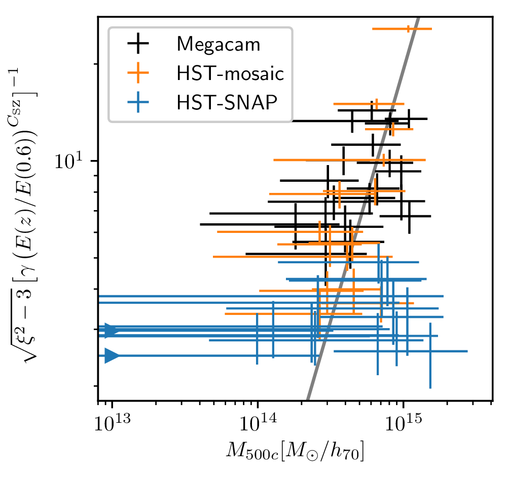
Figure 7: Normalised, debiased, and redshift-evolution-corrected SPT detection significance $\xi$ versus mass. The WL mass estimates are plotted at the best-fitting mass estimate, corrected for mass modelling bias. The error-bars include both shape noise and the scatter in the mass estimates inferred from the simulations. The data points are colour-coded according to the source of the WL data. The solid line shows the best-fit $\zeta$–mass relation. The blue triangles mark clusters from the Snapshot programme which have a best-fitting mass $M_{\mathrm{500c}}<10^{13}\mathrm{M}_{\odot}$.

5.4 The redshift evolution of the $\zeta$–mass relation

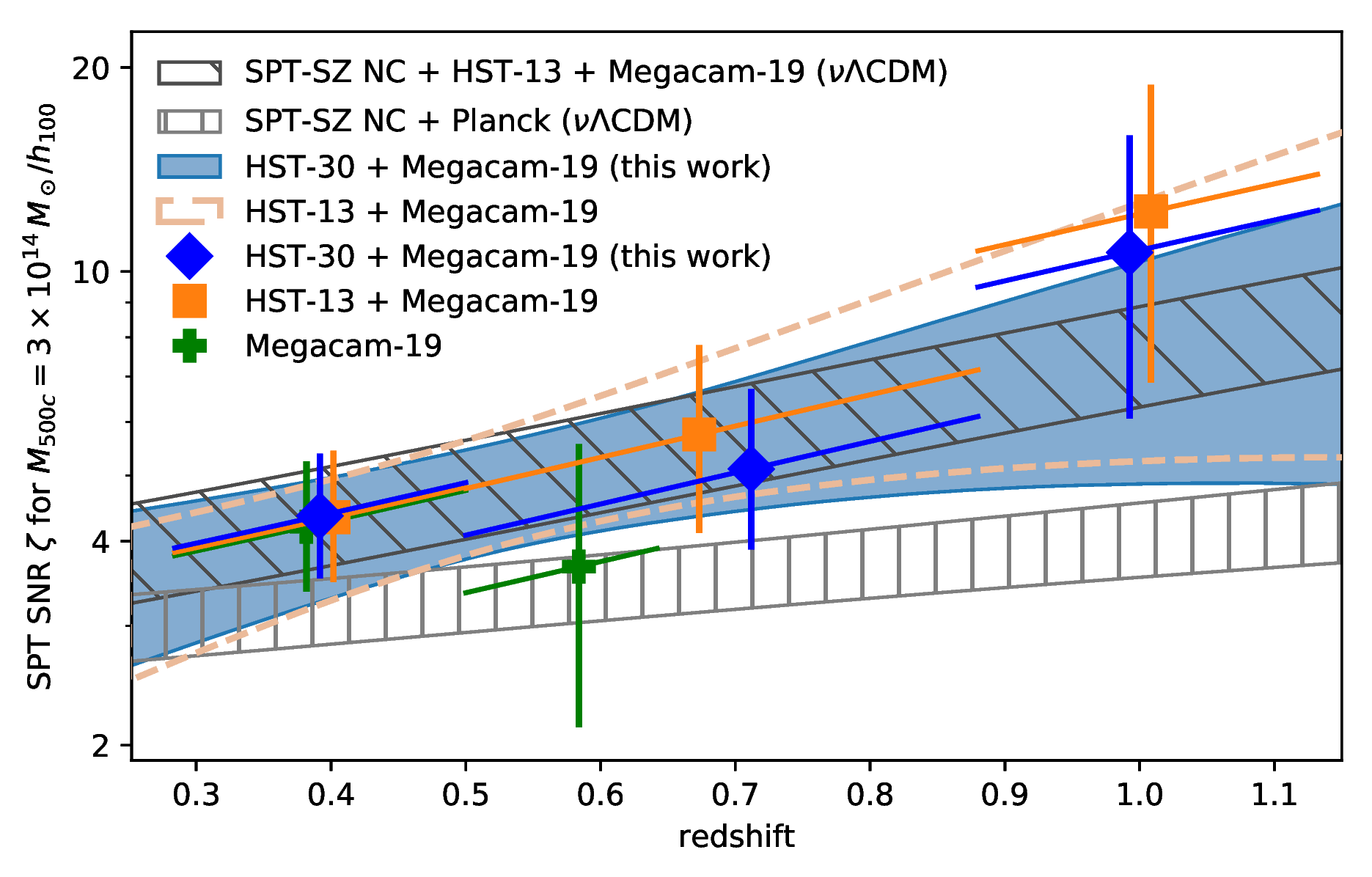
Figure 8: The redshift evolution of the unbiased SPT detection significance $\zeta$ at the pivot mass $3\times 10^{14}\mathrm{M}_{\odot}/h_{100}$. The bands and error bars show the 68% credible interval for the overall relation and the redshift-binned analysis, respectively. Our main analysis is shown in blue, while a corresponding analysis using the WL data employed by B19 is shown in orange. The data points are placed at the mean cluster redshift within each bin. The low-redshift data points are slightly shifted in redshift for better readability. The redshift evolution within each bin is set by ${C_{\mathrm{SZ}}}=1.78$. The hatched regions correspond to the scaling relations derived from the SPT-SZ cluster counts for a Planck $\nu\Lambda$CDM cosmology and the WL-informed SPT cluster cosmology analysis by B19, respectively.

An important result from the previous subsection is that, with our WL data-set, we are able to place a constraint on the redshift evolution ${C_{\mathrm{SZ}}}=1.78\pm 1.11$, albeit weak. We show the evolution of $\zeta$ with redshift in Fig. 8. Coloured bands show the results for the fiducial scaling relation: the predecessor HST-13 + Megacam-19 data-set in orange and the updated data-set from this work in blue. The diagonally-hatched band shows the constraint obtained from a simultaneous analysis of the predecessor HST-13 + Megacam-19 cluster weak-lensing data, X-ray data, and cluster abundance measurements (B19), marginalising over cosmological parameters for a flat $\nu\Lambda$CDM cosmology. Finally, the vertically-hatched band shows the result from a joint analysis of Planck primary CMB anisotropies (TT,TE,EE+lowE, Planck Collaboration et al., 2020b) and the SPT-SZ cluster abundance, also marginalising over cosmological parameters for a flat $\nu\Lambda$CDM cosmology, but without any weak-lensing mass calibration. In this case, the cosmology is essentially set by Planck, and mass calibration is achieved through the cluster abundance likelihood.

We observe an offset between the mass calibration required to match the Planck $\nu\Lambda$CDM cosmology and the mass calibration preferred by our weak-lensing data-set (compare the vertically-hatched band with the blue band in Fig. 8 and the constraints in Table 12). The recovered parameters suggest that, at our pivot redshift $z=0.6$, the WL-preferred mass scale is lower than the mass scale required to match the Planck $\nu\Lambda$CDM cosmology by a factor $0.76^{+0.10}_{-0.14}$. This observation is equivalent to the observation that the parameter constraints on $\Omega_{\mathrm{m}}$ and $\sigma_{8}$ obtained from SPT clusters with WL mass calibration are somewhat lower than the constraints favoured by Planck (see e.g., Bocquet et al. 2015, de Haan et al. 2016, B19).

Because our set of WL clusters spans a rather wide range in redshift, we wish to investigate whether the simple scaling relation model adopted is able to provide a good description of the data. We split our WL clusters into separate redshift bins, limited by $z=0.25,0.5,0.88,1.2$. The bin limits are chosen such that the full sample of 49 clusters has (almost) equal numbers of objects in each of the three bins. We then repeat the scaling relation analysis as discussed above, with the difference that each redshift bin now has its own normalisation parameter $\ln{A_{\mathrm{SZ}}}(z)$. The redshift evolution within each bin is modelled as usual and we fix ${C_{\mathrm{SZ}}}$ to $1.78$, the best-fit result from the full analysis. The parameter constraints are also listed in Table 12. We compare the recovered constraints on $\ln{A_{\mathrm{SZ}}}(z)$ with the result obtained in the fiducial analysis. For each of the three redshift bins, the probability that the recovered amplitude $\ln{A_{\mathrm{SZ}}}(z)$ and the fiducial $\ln{A_{\mathrm{SZ}}}$ are consistent with 0 difference is larger than $p=0.6\,(\text{agreement within }0.5\sigma)$.

In Fig. 8, the data points with error bars show the results from the binned approach we just described. We apply this binned analysis to three WL data combinations: ground-based Magellan/Megacam-19 data (green), the predecessor data-set HST-13 + Megacam-19 (orange), and the full data-set presented in this work (blue). As discussed, we find no evidence that our simple description of the redshift evolution of the SPT observable–mass relation with a single parameter ${C_{\mathrm{SZ}}}$ is in disagreement with the data (compare the blue data points with the blue band in Fig. 8). Note that the slightly larger value of $\ln{A_{\mathrm{SZ}}}$ in the highest-redshift bin would imply that a halo with a given SPT SZ signal would be less massive than implied by the fiducial scaling relation. However, the highest-redshift data points above redshift $\sim 0.9$ are still only weakly constrained and this test thus remains inconclusive.

6 Summary, discussion, and conclusions

In this work we presented weak lensing (WL) measurements for a total sample of 30 distant SPT-SZ clusters based on high-resolution galaxy shape measurements from HST. This includes new observations for 16 clusters using single-pointing ACS F606W images and one cluster with ACS mosaics, as well as a reanalysis of 13 clusters with ACS mosaics. In order to remove cluster galaxies and preferentially select background sources we complemented the single-pointing ACS observations with new Gemini-South GMOS $i$-band imaging (ACS+GMOS sample). For six of the 13 previously studied clusters with ACS mosaics (updated ACS+FORS2 sample) we included new FORS2 $I$-band imaging for the source selection, allowing us to significantly boost the WL source density compared to earlier work. This is not only due to the longer integration times, but also benefited from the excellent image quality of these observations. Studying the source density profiles we confirmed the success of the employed colour selection scheme to remove contaminating cluster galaxies from the source sample. For all targets we employed new calibrations for the source redshift distribution (Raihan et al., 2020) and shear recovery (Hernández-Martín et al., 2020), which also allowed us to include galaxies with slightly lower signal-to-noise ratios in the analysis.

Based on the WL shear measurements we reconstructed the projected mass distributions, yielding clear cluster detections with peak signal-to-noise ratios $S/N_{\mathrm{peak}}>3$ for all clusters with ACS mosaics and eight out of 16 clusters with single-pointing ACS data. In order to constrain the cluster masses we fitted NFW model predictions to the tangential reduced shear profiles, applying corrections for the impact of weak lensing magnification and the finite width of the source redshift distribution. These mass constraints are expected to be biased because of miscentring and variations in cluster density profile. We estimated and corrected for these mass modelling biases using simulated data sets based on the Millennium-XXL simulations (Angulo et al., 2012).

We have used our measurements in combination with earlier WL constraints for lower-redshift clusters from Magellan (D19) to derive refined constraints on the scaling relation between the debiased SPT cluster detection significance $\zeta$ and the cluster mass. In particular, we obtained constraints on the redshift evolution of the scaling relation, which do not rely on information from the cluster counts. While yielding a steeper best-fit power-law index $C_{\mathrm{SZ}}$ for the redshift evolution, our analysis is still consistent with the scaling relation derived from the combination of the SPT clusters counts with earlier WL data (D19, S18) by B19. As a cross-check for the scaling relation analysis we split the clusters into three redshift bins, finding reasonable agreement between the redshift-binned analysis and the overall relation.

We have not yet used our expanded high-$z$ WL data set to derive improved cosmological constraints from SPT clusters, but postpone this to future work, which will also incorporate additional WL data for clusters at lower redshifts. However, we have compared our WL-derived scaling relation constraints to the scaling relation that would be expected from the SPT cluster counts in a flat Planck $\nu\Lambda$CDM cosmology (compare Fig. 8). In all redshift bins the WL-based analysis yields higher $\zeta$ at a given reference mass, consistent with the previously reported offset in the best-fit $\sigma_{8}$ estimates between Planck and SPT clusters (B19). However, the overall significance of the discrepancy is still low, which is why larger WL data sets will be needed to sensitively test the level of agreement between SPT clusters and Planck CMB constraints.

Compared to the earlier work from S18 we were able to reduce the total systematic uncertainty for the analysis of clusters with ACS mosaics, for which we can use X-ray centroids to centre the WL reduced shear profiles, from 9.2% to 7.5%, mostly due to our smaller shear calibration uncertainty. Now the largest contribution to the systematic error budget comes from residual uncertainties in the mass modelling correction. This is even more severe for the clusters in our ACS+GMOS sample for two reasons. First, their smaller field of view (single ACS pointing) limits the constraints to scales $r\lesssim 900\,$kpc. Although we generally exclude the cluster cores ($r<500\,$kpc) from our analysis, this still amplifies the impact especially of miscentring uncertainties. In addition, nearly all of the clusters currently lack high-resolution X-ray observations, which would provide a tighter centre proxy than the SZ peak positions. As a result, the analysis of these data is currently subject to a 11.6% total systematic uncertainty, which is dominated by mass modelling uncertainties.

While systematic errors do not yet dominate our total error budget, it will be crucial to reduce them for future WL analyses of larger samples of massive high-$z$ clusters. As one step to reduce mass modelling uncertainties, X-ray centres should become available for large samples of massive clusters in the near future from eROSITA (Merloni et al., 2012). In addition, it will be important to reduce uncertainties in our understanding of miscentring distributions. One route for this is given by the comparison of different centre proxies. E.g., Zhang et al. (2019) compare the centres derived from the redMaPPer cluster finding algorithm to X-ray centres. This was also done by Bleem et al. (2020), who furthermore compared redMaPPer and SZ centres. However, even X-ray centres do not exactly correspond to the 3D halo centres. As argued by S18, a possible solution could be provided by studying offset distributions between centre proxies (from X-ray, SZ, or optical data) and weak lensing mass peaks (which provide noisy tracers for the 3D halo centre, Dietrich et al., 2012), and comparing these distributions between the real data and mock data from hydrodynamical simulations with matched noise properties. The two noisy distributions should agree if the hydrodynamical simulations accurately describe the true miscentring.

As a further approach to reduce mass modelling uncertainties we recommend to generally obtain observations with a larger field of view (e.g. the $2\times 2$ ACS mosaics studied here) when obtaining pointed follow-up for massive high-$z$ clusters. In addition to reducing systematic uncertainties this also reduces the weak lensing fit uncertainties and the intrinsic scatter (compare Tables 8 and 9).

For clusters at redshifts $0.7\lesssim z\lesssim 1.0$ a more cost-effective alternative to HST mosaics may be provided by deep good-seeing ground-based $K_{\mathrm{s}}$ imaging. This also has the benefit of reducing systematic uncertainties related to the calibration of the redshift distribution compared to the source selection scheme applied in this paper (Schrabback et al., 2018b). We however stress that the depth and the resolution of HST observations (including NIR imaging for the source selection) are still critically needed for weak lensing measurements of massive clusters at $z>1$.

Samples of massive, well-selected clusters that extend out to high redshifts have been increasing rapidly in recent years (e.g. Hilton et al., 2018, 2021; Bleem et al., 2020; Huang et al., 2020), and will continue to do so thanks to the latest surveys, including the one conducted by eROSITA (Merloni et al., 2012). In order to exploit their full potential for constraints on dark energy properties and other cosmological parameters it will be crucial to further tighten the cluster mass calibration by reducing systematic uncertainties and adding new WL data. This includes for example the observations conducted by Euclid (Laureijs et al., 2011) and the Vera C. Rubin Observatory (LSST Science Collaboration et al., 2009), especially for the calibration of more common intermediate-mass clusters, as well as further deep high-resolution follow-up for rare high-mass, high-$z$ clusters.

Data availability

SPT cluster data products are available at https://pole.uchicago.edu/public/data/sptsz-clusters/. The scaling relation pipeline used in our analysis is available at https://github.com/SebastianBocquet/SPT_SZ_cluster_likelihood. It will be updated to include the tangential reduced shear profiles and source redshift distributions derived in our analysis once this paper is accepted.

Affiliations

¹ Argelander-Institut für Astronomie, Universität Bonn, Auf dem Hügel 71, 53121, Bonn, Germany
² Faculty of Physics, Ludwig-Maximilians University, Scheinerstr. 1, 81679 München, Germany
³ Excellence Cluster ORIGINS, Boltzmannstr. 2, 85748 Garching, Germany
⁴ Ruhr-University Bochum, Astronomical Institute, German Centre for Cosmological Lensing, Universitätsstr. 150, 44801 Bochum, Germany
⁵ Leiden Observatory, Leiden University, Niels Bohrweg 2, NL-2300 CA Leiden, The Netherlands
⁶ Max-Planck-Institut für Astronomie, Königstuhl 17, D-69117 Heidelberg, Germany
⁷ Kavli Institute for Cosmological Physics, University of Chicago, 5640 South Ellis Avenue, Chicago, IL 60637
⁸ Department of Physics, University of Cincinnati, Cincinnati, OH 45221, USA
⁹ Fermi National Accelerator Laboratory, Batavia, IL 60510-0500, USA
¹⁰ Department of Astronomy and Astrophysics, University of Chicago, 5640 South Ellis Avenue, Chicago, IL 60637
¹¹ Department of Physics, University of Chicago, 5640 South Ellis Avenue, Chicago, IL 60637
¹² Argonne National Laboratory, 9700 S. Cass Avenue, Argonne, IL, USA 60439
¹³ Department of Physics and Astronomy, University of Missouri–Kansas City, 5110 Rockhill Road, Kansas City, MO 64110, USA
¹⁴ Département de Physique, Université de Montréal, Montréal, QC, Canada
¹⁵ MIT Kavli Institute for Astrophysics and Space Research, Massachusetts Institute of Technology, 77 Massachusetts Avenue, Cambridge, MA 02139
¹⁶ Astronomy Unit, Department of Physics, University of Trieste, via Tiepolo 11, I-34131 Trieste, Italy
¹⁷ IFPU - Institute for Fundamental Physics of the Universe, Via Beirut 2, 34014 Trieste, Italy
¹⁸ INAF - Osservatorio Astronomico di Trieste, via G. B. Tiepolo 11, I-34143 Trieste, Italy
¹⁹ INFN - National Institute for Nuclear Physics, Via Valerio 2, I-34127 Trieste, Italy
²⁰ Center for Astrophysics $|$ Harvard & Smithsonian 60 Garden Street $|$ MS 42 $|$ Cambridge, MA 02138

Appendix A Dependence of the average geometric lensing efficiency on galaxy size

Figure 9: Dependence of the estimated $\langle\beta\rangle$ for SPT-CL $J$0000$-$5748 on the galaxy flux radius $r_{\mathrm{f}}$, including all galaxies with $24<V<26.5$ that pass the ACS-only colour selection, averaged over the five CANDELS fields (solid curve). The dashed curve indicates the fraction of the summed shape weights of the galaxies located within the corresponding bin (width $\Delta r_{\mathrm{f}}=0.5$ pixels).

Following the ACS-only colour selection and including all galaxies with $24<V<26.5$, Fig. 9 shows the dependence of the estimated $\langle\beta\rangle$ for SPT-CL J0000$-$5748 on the galaxy flux radius $r_{\mathrm{f}}$. The dashed curve in the figure represents the fraction of the summed shape weights of the galaxies that are located within the corresponding $r_{\mathrm{f}}$ bin. This shows that most galaxies are located in the regime $r_{\mathrm{f}}\lesssim 5$ pixels, where $\langle\beta\rangle$ depends only weakly on $r_{\mathrm{f}}$.

Appendix B Cross-check from overlapping shear estimates

The cluster SPT-CL $J$2043$-$5035 has been observed by two separate HST programmes (see Sect. 2.1.1). For this target we have therefore computed ACS F606W shape measurements from both the $2\times 2$ ACS mosaic and the central single pointing observation. This provides us with an opportunity to cross-check our shape measurements in the overlap region. The difference profiles between the two reduced shear estimates is shown in Fig. 10, decomposed into tangential and cross-components with respect to the cluster centre. For the tangential component (which is used to constrain the mass models, see Sect. 4), the difference profile is well consistent with zero, as expected. For the cross-component the difference is slightly positive on average, but combining the different radial bins the deviation from zero is significant at the $\sim 1.6\sigma$ level only, which is therefore not a concern. Note that for galaxies with two successful shear estimates we use the average of the two estimates in the actual cluster WL analysis (see Sect. 4).

Figure 10: Difference in the reduced tangential shear (black solid points) and the cross shear (grey open points, shifted along the $x$-axis for clarity) estimates from the ACS mosaic versus the single-pointing SNAP observation of SPT-CL $J$2043$-$5035, computed using only galaxies that are present in both catalogues and plotted as a function of distance from the SZ centre. The outlier at $r=0.75$ Mpc is dominated by a single noisy galaxy with complex morphology. For this figure error-bars have been computed by randomising the phases of the ellipticity differences. The actual reduced tangential and cross shear profiles of the cluster are shown in Fig. 12.

Appendix C Miscentring distributions

To correct our weak lensing mass estimates for the impact of miscentring (see Sect. 4.3) we employ miscentring distributions for the X-ray centroids and SZ peaks which are based on the Magneticum Pathfinder Simulation (Dolag, Komatsu & Sunyaev, 2016). These distributions were already employed in S18 and are shown in Fig. 11. In this Appendix we briefly summarise how these distributions were derived.

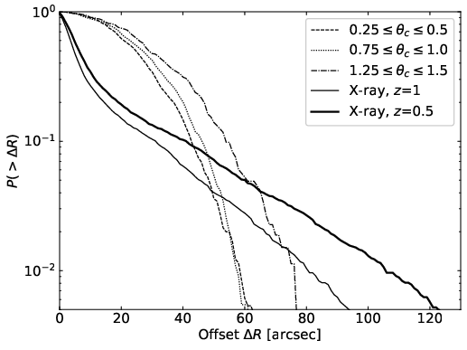
Figure 11: Cumulative offset distribution measured between the deepest point in the halo potential and centre proxies in the SPT-SZ mock observations. The dashed, dotted, and dash-dotted curves correspond to SZ centres for simulated clusters with core sizes in the ranges $0\aas@@fstack{\prime}25\leq\theta_{\mathrm{c}}\leq 0\aas@@fstack{\prime}5$, $0\aas@@fstack{\prime}75\leq\theta_{\mathrm{c}}\leq 1\aas@@fstack{\prime}0$, and $1\aas@@fstack{\prime}25\leq\theta_{\mathrm{c}}\leq 1\aas@@fstack{\prime}5$, which have r.m.s. offsets of $29^{\prime\prime}$, $31^{\prime\prime}$, and $36^{\prime\prime}$, respectively. The solid curves correspond to X-ray centres, whose r.m.s. offset of 159 kpc equals $20^{\prime\prime}$ at $z=1$ (thin curve) and $26^{\prime\prime}$ at $z=0.5$ (thick curve).

The large-volume, high-resolution cosmological hydrodynamical Magneticum Pathfinder simulations were carried out with P-GADGET3, a modification of P-GADGET-2 (Springel, 2005), using an entropy-conserving formulation of Smoothed Particle Hydrodynamics (SPH, Springel & Hernquist, 2002) and including treatment of radiative cooling, heating by a UV background, star formation and feedback processes from supernovae explosions and active galactic nuclei (Springel & Hernquist, 2003; Fabjan et al., 2010). From this set of simulations Saro et al. (2014) and Gupta et al. (2017) employed a high-resolution simulation, which is based on a WMAP7 cosmology (Komatsu et al., 2011) and contains $1512^{3}$ dark matter particles and as many gas particles in a comoving box of $896h^{-1}$ Mpc per side, to create thermal Sunyaev-Zel’dovich Effect (SZE) light cones and SPT mock observations. To replicate the observing conditions of the SPT-SZ survey they built five thermal SZE light-cones up to $z\sim 2$, each of size $13\deg\times 13\deg$, from which mock SPT observations at 95 GHz and 150 GHz were extracted. In each mock, they accounted for three contributions: (1) primary CMB anisotropies; (2) the SPT beam and transfer function (Schaffer et al., 2011) at the two frequencies; (3) instrumental noise consistent with the observed SPT-SZ map depths of 18 and 44 $\mu$K-arcmin for the 150 GHz and 95 GHz bands, respectively. From these mocks, cluster candidates were identified with the same approach adopted for real SPT clusters (e.g. Staniszewski et al., 2009; Reichardt et al., 2013; Bleem et al., 2020). In particular, a $\beta$-profile (Cavaliere & Fusco-Femiano, 1976) with $\beta=1$ was used as a cluster template, and different cluster core sizes $\theta_{\mathrm{c}}$ were adopted, also in line with the SPT data analysis, with twelve discrete values evenly spaced in the range $0\aas@@fstack{\prime}25$–$3\aas@@fstack{\prime}0$ (only values $\leq 1\aas@@fstack{\prime}5$ are relevant for the present analysis). The resulting sample of SPT-SZ-like clusters (selected to have detection significances $\xi>4.5$) was used to characterise both the SZE and X-ray miscentring distributions. These were computed with respect to the deepest point in the potential of the halo, which is the centre typically used for computations of the halo mass function (e.g. Bocquet et al., 2020). The SZ centres directly correspond to the SZ peak location, as employed for the real survey data. X-ray centres were defined as the peak in the X-ray surface brightness maps within a radius of $2r_{\mathrm{500c}}$ around the deepest point of the potential.

The resulting offset distributions are shown in Fig. 11. We find that the SZ miscentring mostly depends on the cluster core size $\theta_{\mathrm{c}}$. We therefore compute and employ separate offset distributions for each of the discrete $\theta_{\mathrm{c}}$ values. The X-ray offset distribution is measured in transverse physical separation, leading to a redshift dependence of the offset distribution in angular separation (see Fig. 11). In most cases the simulated X-ray centres trace the halo centres with smaller offsets compared to the SZ centres, leading to smaller mass modelling bias corrections. However, there is a slightly increased tail towards large offsets for the X-ray centres, especially at lower cluster redshifts. For parametric fits to the SZ miscentring distribution in this simulation see Gupta et al. (2017).

Appendix D Weak lensing results for individual clusters

In this Appendix we present the mass reconstructions and shear profiles of the individual clusters as described in Sections 4.1 and 4.2. These figures are available as supplementary material.

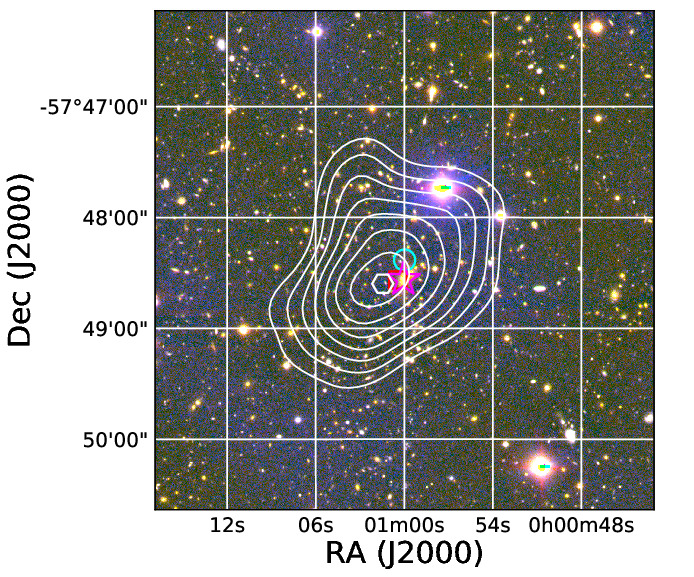
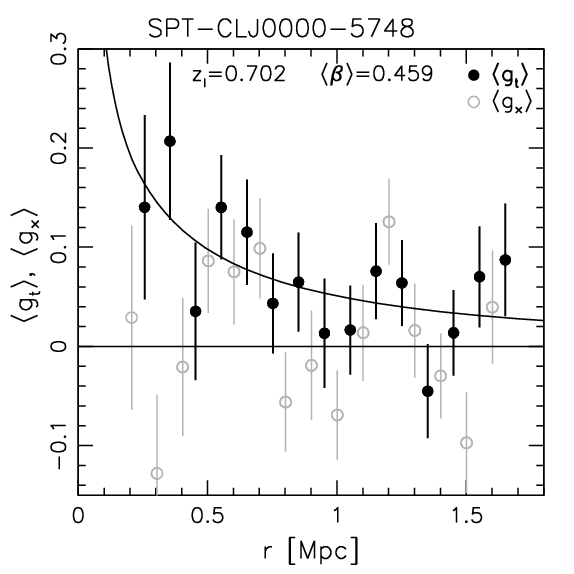
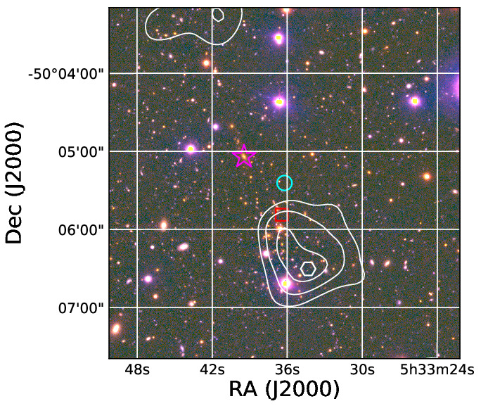
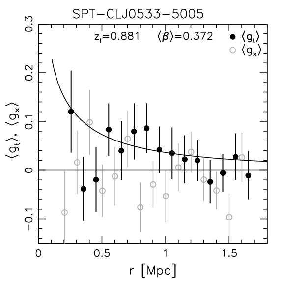
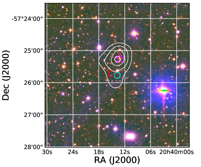
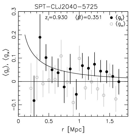
Figure 13: WL results for clusters from the updated ACS+FORS2 sample. Left: Signal-to-noise ratio map of the WL mass reconstruction (starting at $2\sigma$ in steps of $0.5\sigma$, with the peak indicated by the hexagon), overlaid on a VLT/FORS2 $zIB$ colour image ($4\aas@@fstack{\prime}5\times 4\aas@@fstack{\prime}5$ cutout, using $z$- and $B$-band images from Chiu et al., 2016). The BCG (from Chiu et al., 2016), SZ peak, and X-ray centroid are shown by the magenta star, cyan circle, and red square, respectively. Right: Combined reduced shear profile around the X-ray centre, showing the tangential (black solid circles with best-fitting NFW model) and cross (grey open circles, shifted along the $x$-axis for clarity) components.

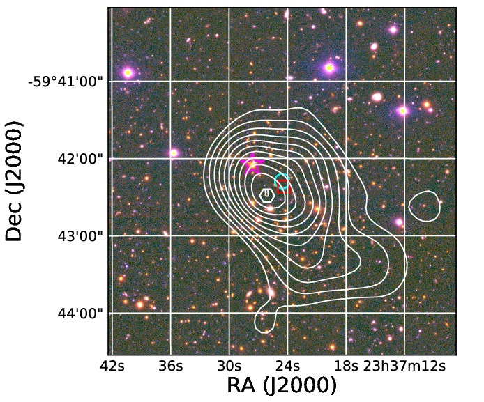
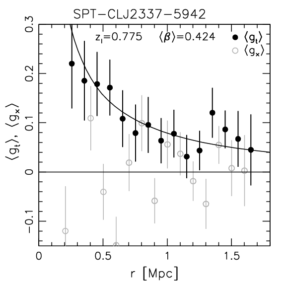
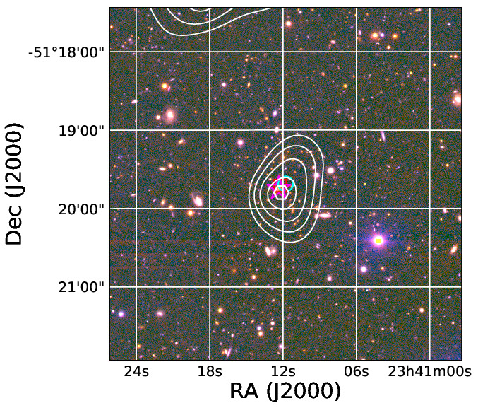
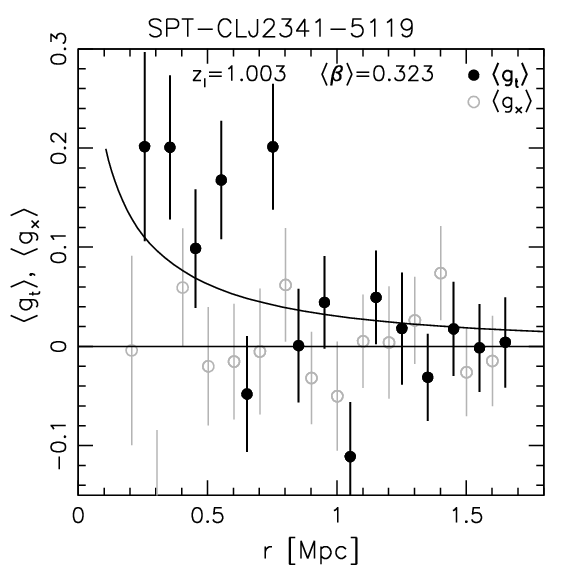
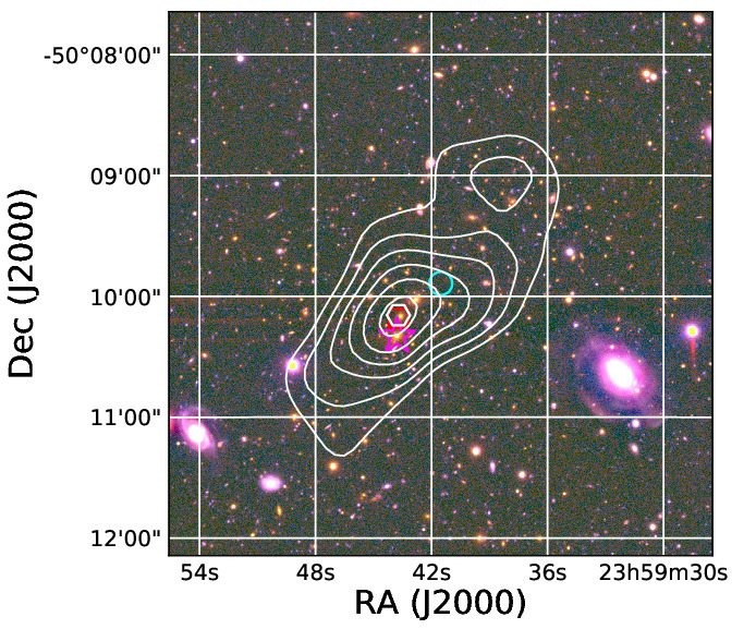
Figure 14: WL results for clusters from the updated ACS+FORS2 sample (continued, see Fig. 13 for details).

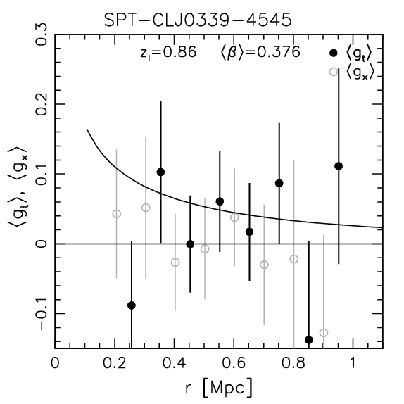
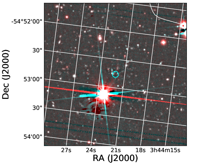
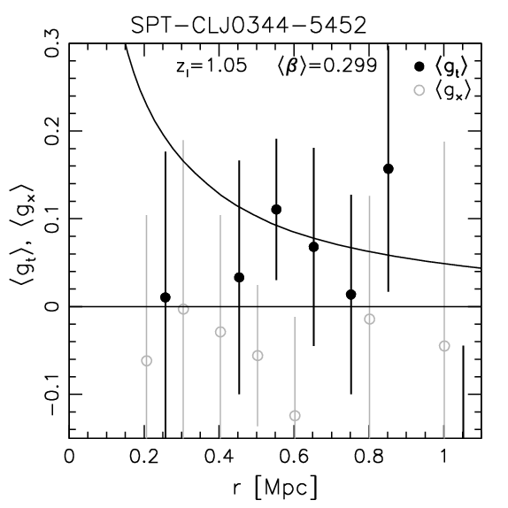
Figure 16: WL results for clusters from the ACS+GMOS sample (continued, see Fig. 15 for details).

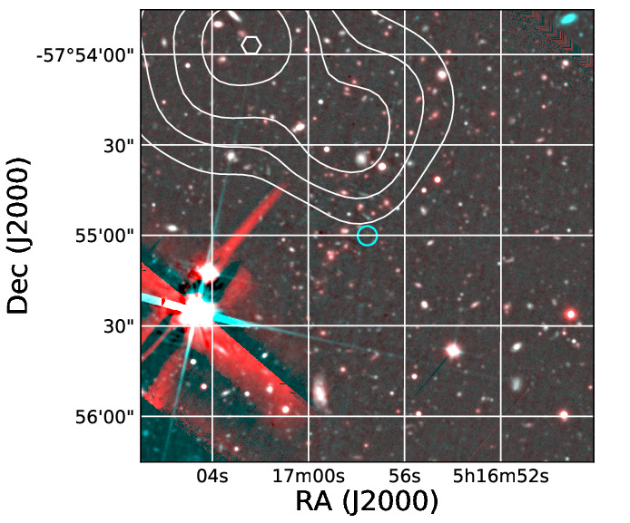
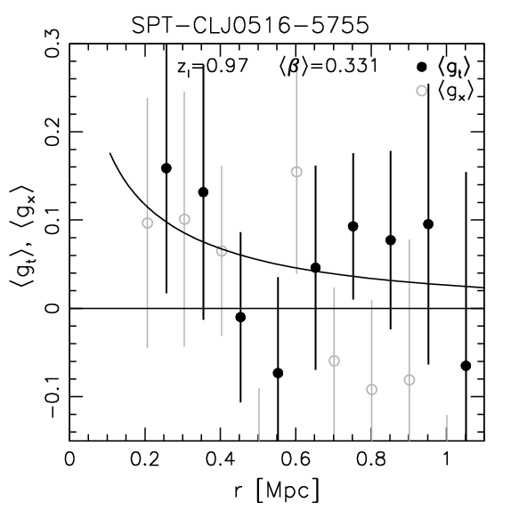
Figure 18: WL results for clusters from the ACS+GMOS sample (continued, see Fig. 15 for details). We stress that the regions affected by bright stars (especially in the GMOS images) are well masked in our analysis. We therefore expect that the apparent alignment of a bright star with the peak in the signal-to-noise ratio map of the WL mass reconstruction for SPT-CL $J$0422$-$4608 is purely by chance.

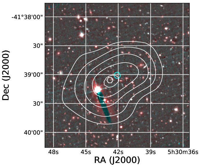
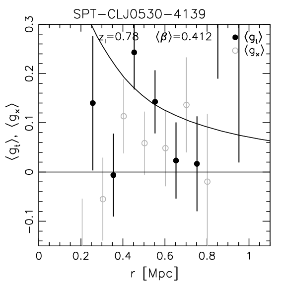
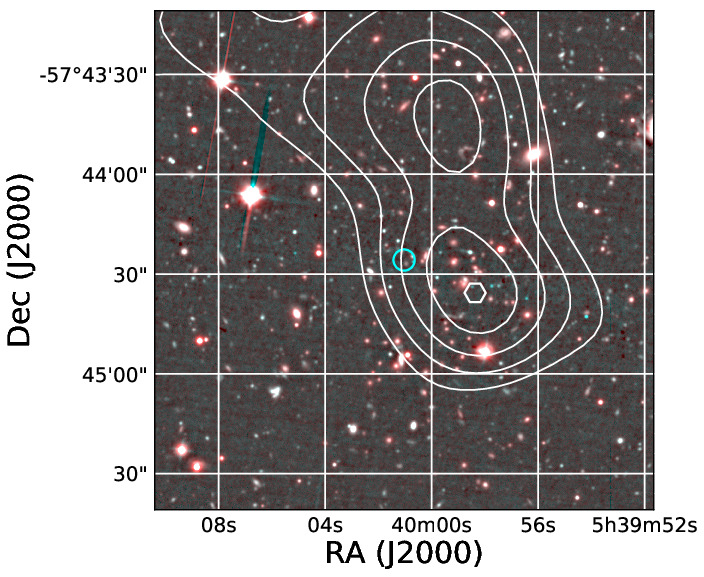
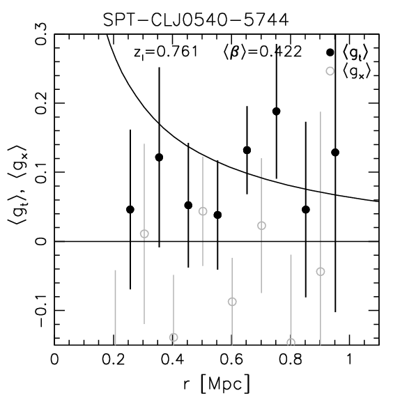
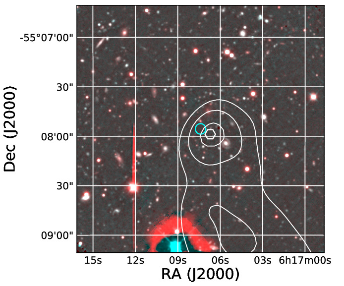
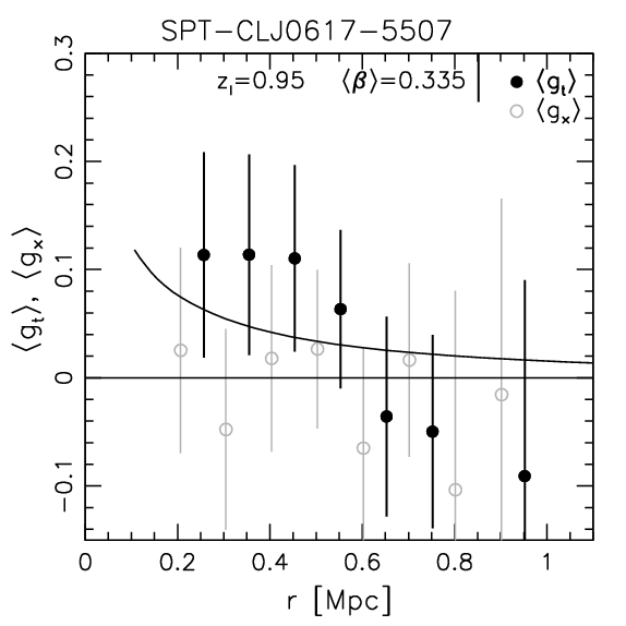
Figure 19: WL results for clusters from the ACS+GMOS sample (continued, see Fig. 15 for details).

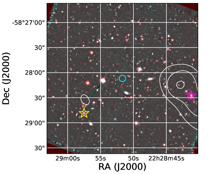
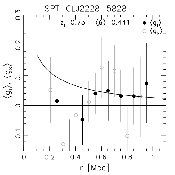
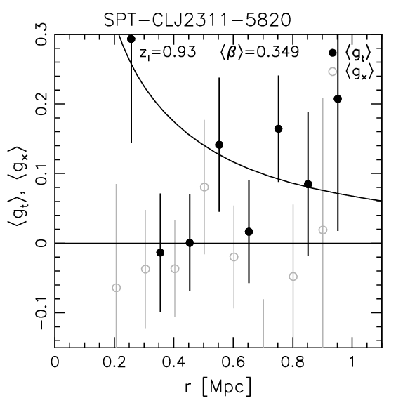
Figure 20: WL results for clusters from the ACS+GMOS sample (continued, see Fig. 15 for details). As an exception, we show a slightly larger ($3^{\prime}\times 3^{\prime}$) cut-out for SPT-CL $J$2228$-$5828 (top left), where we also mark the BCG candidate from Zenteno et al. (2020) and the brightest galaxy in a secondary concentration of candidate cluster galaxies ($\alpha=337.2396\thinspace$deg, $\delta=-58.4801\thinspace$deg) with the magenta and yellow stars, respectively (see also footnote 9). The cyan dots visible near the corners of this image are residual cosmic rays and other image reduction artefacts, which occur close to the edge of the ACS field-of-view, but are masked in the science analysis.

References

- Allen, Evrard & Mantz (2011) Allen S. W., Evrard A. E., Mantz A. B., 2011, ARA&A, 49, 409
- Angulo et al. (2012) Angulo R. E., Springel V., White S. D. M., Jenkins A., Baugh C. M., Frenk C. S., 2012, MNRAS, 426, 2046
- Applegate et al. (2014) Applegate D. E. et al., 2014, MNRAS, 439, 48
- Bartelmann & Schneider (2001) Bartelmann M., Schneider P., 2001, Phys. Rep., 340, 291
- Bayliss et al. (2016) Bayliss M. B. et al., 2016, ApJS, 227, 3
- Becker & Kravtsov (2011) Becker M. R., Kravtsov A. V., 2011, ApJ, 740, 25
- Benítez (2000) Benítez N., 2000, ApJ, 536, 571
- Bertin & Arnouts (1996) Bertin E., Arnouts S., 1996, A&AS, 117, 393
- Bleem et al. (2020) Bleem L. E. et al., 2020, ApJS, 247, 25
- Bleem et al. (2015) Bleem L. E. et al., 2015, ApJS, 216, 27
- Bocquet et al. (2019) Bocquet S. et al., 2019, ApJ, 878, 55
- Bocquet et al. (2020) Bocquet S., Heitmann K., Habib S., Lawrence E., Uram T., Frontiere N., Pope A., Finkel H., 2020, ApJ, 901, 5
- Bocquet et al. (2015) Bocquet S. et al., 2015, ApJ, 799, 214
- Boffin, Moehler & Freudling (2016) Boffin H., Moehler S., Freudling W., 2016, The Messenger, 163, 10
- Brammer, van Dokkum & Coppi (2008) Brammer G. B., van Dokkum P. G., Coppi P., 2008, ApJ, 686, 1503
- Brammer et al. (2012) Brammer G. B. et al., 2012, ApJS, 200, 13
- Brammer et al. (2013) Brammer G. B., van Dokkum P. G., Illingworth G. D., Bouwens R. J., Labbé I., Franx M., Momcheva I., Oesch P. A., 2013, ApJ, 765, L2
- Carlstrom et al. (2011) Carlstrom J. E. et al., 2011, PASP, 123, 568
- Cavaliere & Fusco-Femiano (1976) Cavaliere A., Fusco-Femiano R., 1976, A&A, 49, 137
- Child et al. (2018) Child H. L., Habib S., Heitmann K., Frontiere N., Finkel H., Pope A., Morozov V., 2018, ApJ, 859, 55
- Chiu et al. (2016) Chiu I. et al., 2016, MNRAS, 455, 258
- de Haan et al. (2016) de Haan T. et al., 2016, ApJ, 832, 95
- Diemer & Joyce (2019) Diemer B., Joyce M., 2019, ApJ, 871, 168
- Dietrich et al. (2019) Dietrich J. P. et al., 2019, MNRAS, 483, 2871
- Dietrich et al. (2012) Dietrich J. P., Böhnert A., Lombardi M., Hilbert S., Hartlap J., 2012, MNRAS, 419, 3547
- Dodelson et al. (2016) Dodelson S., Heitmann K., Hirata C., Honscheid K., Roodman A., Seljak U., Slosar A., Trodden M., 2016, arXiv:1604.07626
- Dolag, Komatsu & Sunyaev (2016) Dolag K., Komatsu E., Sunyaev R., 2016, MNRAS, 463, 1797
- Erben et al. (2005) Erben T. et al., 2005, Astronomische Nachrichten, 326, 432
- Erben et al. (2001) Erben T., Van Waerbeke L., Bertin E., Mellier Y., Schneider P., 2001, A&A, 366, 717
- Euclid Collaboration: Martinet et al. (2019) Euclid Collaboration: Martinet N. et al., 2019, A&A, 627, A59
- Fabjan et al. (2010) Fabjan D., Borgani S., Tornatore L., Saro A., Murante G., Dolag K., 2010, MNRAS, 401, 1670
- Feroz, Hobson & Bridges (2009) Feroz F., Hobson M. P., Bridges M., 2009, MNRAS, 398, 1601
- Grogin et al. (2011) Grogin N. A. et al., 2011, ApJS, 197, 35
- Gupta et al. (2017) Gupta N., Saro A., Mohr J. J., Dolag K., Liu J., 2017, MNRAS, 469, 3069
- Herbonnet et al. (2020) Herbonnet R. et al., 2020, MNRAS, 497, 4684
- Hernández-Martín et al. (2020) Hernández-Martín B. et al., 2020, A&A, 640, A117
- Hilton et al. (2018) Hilton M. et al., 2018, ApJS, 235, 20
- Hilton et al. (2021) Hilton M. et al., 2021, ApJS, 253, 3
- Hinshaw et al. (2013) Hinshaw G. et al., 2013, ApJS, 208, 19
- Hoekstra, Franx & Kuijken (2000) Hoekstra H., Franx M., Kuijken K., 2000, ApJ, 532, 88
- Hoekstra et al. (1998) Hoekstra H., Franx M., Kuijken K., Squires G., 1998, ApJ, 504, 636
- Hoekstra et al. (2015) Hoekstra H., Herbonnet R., Muzzin A., Babul A., Mahdavi A., Viola M., Cacciato M., 2015, MNRAS, 449, 685
- Huang et al. (2020) Huang N. et al., 2020, AJ, 159, 110
- Inami et al. (2017) Inami H. et al., 2017, A&A, 608, A2
- Jee et al. (2011) Jee M. J. et al., 2011, ApJ, 737, 59
- Jee et al. (2017) Jee M. J., Ko J., Perlmutter S., Gonzalez A., Brodwin M., Linder E., Eisenhardt P., 2017, ApJ, 847, 117
- Kaiser & Squires (1993) Kaiser N., Squires G., 1993, ApJ, 404, 441
- Kaiser, Squires & Broadhurst (1995) Kaiser N., Squires G., Broadhurst T., 1995, ApJ, 449, 460
- Kim et al. (2019) Kim J., Jee M. J., Perlmutter S., Hayden B., Rubin D., Huang X., Aldering G., Ko J., 2019, ApJ, 887, 76
- Koekemoer et al. (2011) Koekemoer A. M. et al., 2011, ApJS, 197, 36
- Koekemoer et al. (2003) Koekemoer A. M., Fruchter A. S., Hook R. N., Hack W., 2003, in HST Calibration Workshop : Hubble after the Installation of the ACS and the NICMOS Cooling System, Arribas S., Koekemoer A., Whitmore B., eds., p. 337
- Komatsu et al. (2011) Komatsu E. et al., 2011, ApJS, 192, 18
- Laureijs et al. (2011) Laureijs R. et al., 2011, arXiv:1110.3193
- Lee et al. (2018) Lee B. E., Le Brun A. M. C., Haq M. E., Deering N. J., King L. J., Applegate D., McCarthy I. G., 2018, MNRAS, 479, 890
- LSST Science Collaboration et al. (2009) LSST Science Collaboration et al., 2009, arXiv:0912.0201
- Luppino & Kaiser (1997) Luppino G. A., Kaiser N., 1997, ApJ, 475, 20
- Mahler et al. (2020) Mahler G. et al., 2020, ApJ, 894, 150
- Mantz et al. (2015) Mantz A. B. et al., 2015, MNRAS, 446, 2205
- Massey et al. (2014) Massey R. et al., 2014, MNRAS, 439, 887
- McClintock et al. (2019) McClintock T. et al., 2019, MNRAS, 482, 1352
- McDonald et al. (2019) McDonald M. et al., 2019, ApJ, 870, 85
- McDonald et al. (2013) McDonald M. et al., 2013, ApJ, 774, 23
- McInnes et al. (2009) McInnes R. N., Menanteau F., Heavens A. F., Hughes J. P., Jimenez R., Massey R., Simon P., Taylor A., 2009, MNRAS, 399, L84
- Merloni et al. (2012) Merloni A. et al., 2012, arXiv:1209.3114
- Miyatake et al. (2019) Miyatake H. et al., 2019, ApJ, 875, 63
- Moehler et al. (2010) Moehler S., Freudling W., Møller P., Patat F., Rupprecht G., O’Brien K., 2010, PASP, 122, 93
- Momcheva et al. (2016) Momcheva I. G. et al., 2016, ApJS, 225, 27
- Murata et al. (2019) Murata R. et al., 2019, PASJ, 71, 107
- Navarro, Frenk & White (1997) Navarro J. F., Frenk C. S., White S. D. M., 1997, ApJ, 490, 493
- Okabe & Smith (2016) Okabe N., Smith G. P., 2016, MNRAS, 461, 3794
- Planck Collaboration et al. (2020a) Planck Collaboration et al., 2020a, A&A, 641, A6
- Planck Collaboration et al. (2020b) Planck Collaboration et al., 2020b, A&A, 641, A5
- Rafelski et al. (2015) Rafelski M. et al., 2015, AJ, 150, 31
- Raihan et al. (2020) Raihan S. F., Schrabback T., Hildebrandt H., Applegate D., Mahler G., 2020, MNRAS, 497, 1404
- Reichardt et al. (2013) Reichardt C. L. et al., 2013, ApJ, 763, 127
- Rowe et al. (2015) Rowe B. T. P. et al., 2015, Astronomy and Computing, 10, 121
- Saro et al. (2014) Saro A. et al., 2014, MNRAS, 440, 2610
- Schaffer et al. (2011) Schaffer K. K. et al., 2011, ApJ, 743, 90
- Schirmer (2013) Schirmer M., 2013, ApJS, 209, 21
- Schlegel, Finkbeiner & Davis (1998) Schlegel D. J., Finkbeiner D. P., Davis M., 1998, ApJ, 500, 525
- Schneider (2006) Schneider P., 2006, in: Gravitational Lensing: Strong, Weak & Micro, Saas-Fee Advanced Course 33, Swiss Society for Astrophysics and Astronomy, G. Meylan, P. Jetzer & P. North (Eds.), Springer-Verlag: Berlin, p. 269, Springer-Verlag: Berlin
- Schneider & Seitz (1995) Schneider P., Seitz C., 1995, A&A, 294, 411
- Schrabback et al. (2018a) Schrabback T. et al., 2018a, MNRAS, 474, 2635
- Schrabback et al. (2007) Schrabback T. et al., 2007, A&A, 468, 823
- Schrabback et al. (2010) Schrabback T. et al., 2010, A&A, 516, A63
- Schrabback et al. (2018b) Schrabback T. et al., 2018b, A&A, 610, A85
- Seitz & Schneider (1997) Seitz C., Schneider P., 1997, A&A, 318, 687
- Simon (2012) Simon P., 2012, A&A, 543, A2
- Simon, Taylor & Hartlap (2009) Simon P., Taylor A. N., Hartlap J., 2009, MNRAS, 399, 48
- Skelton et al. (2014) Skelton R. E. et al., 2014, ApJS, 214, 24
- Sommer et al. (2021) Sommer M. W., Schrabback T., Applegate D. E., Hilbert S., Ansarinejad B., Floyd B., Grandis S., 2021, MNRAS submitted (also arXiv:2105.08027)
- Springel (2005) Springel V., 2005, MNRAS, 364, 1105
- Springel & Hernquist (2002) Springel V., Hernquist L., 2002, MNRAS, 333, 649
- Springel & Hernquist (2003) Springel V., Hernquist L., 2003, MNRAS, 339, 289
- Staniszewski et al. (2009) Staniszewski Z. et al., 2009, ApJ, 701, 32
- Stern et al. (2019) Stern C. et al., 2019, MNRAS, 485, 69
- Sunyaev & Zel’dovich (1970) Sunyaev R. A., Zel’dovich Y. B., 1970, Comments on Astrophysics and Space Physics, 2, 66
- Sunyaev & Zel’dovich (1972) Sunyaev R. A., Zel’dovich Y. B., 1972, Comments on Astrophysics and Space Physics, 4, 173
- Swetz et al. (2011) Swetz D. S. et al., 2011, ApJS, 194, 41
- Thölken et al. (2018) Thölken S. et al., 2018, A&A, 610, A71
- Tinker et al. (2008) Tinker J., Kravtsov A. V., Klypin A., Abazajian K., Warren M., Yepes G., Gottlöber S., Holz D. E., 2008, ApJ, 688, 709
- Umetsu et al. (2020) Umetsu K. et al., 2020, ApJ, 890, 148
- Vanderlinde et al. (2010) Vanderlinde K. et al., 2010, ApJ, 722, 1180
- von der Linden et al. (2014) von der Linden A. et al., 2014, MNRAS, 439, 2
- Wolf (2009) Wolf C., 2009, MNRAS, 397, 520
- Wright & Brainerd (2000) Wright C. O., Brainerd T. G., 2000, ApJ, 534, 34
- Zenteno et al. (2020) Zenteno A. et al., 2020, MNRAS, 495, 705
- Zhang et al. (2019) Zhang Y. et al., 2019, MNRAS, 488, 1
- Zuntz et al. (2015) Zuntz J. et al., 2015, Astronomy and Computing, 12, 45