Degeneration of Topological String partition functions and Mirror curves of the Calabi-Yau threefolds $X_{N,M}$

Abstract

In this article we study certain degenerations of the mirror curves associated with the Calabi-Yau threefolds $X_{N,M}$, and the effect of these degenerations on the refined topological string partition function of $X_{N,M}$. We show that when the mirror curve degenerates and become the union of the lower genus curves the corresponding partition function factorizes into pieces corresponding to the components of the degenerate mirror curve. Moreover we show that using degeneration of a generalised mirror curve it is possible to obtain the partition function corresponding to $X_{N,M-1}$ from $X_{N,M}$.

1 Introduction: Refined topological strings on $X_{N,M}$ and corresponding Mirror Curves

The non-compact Calabi-Yau threefold (CY threefold) $X_{N,M}$ with $N,M\in\mathbb{N}$ Hohenegger:2016eqy ; Bastian:2017ary ; Ahmed:2017hfr ; Haghighat:2018gqf ; Hohenegger:2013ala ; Hohenegger:2016yuv ; Hohenegger:2015btj ; Deger:2018kur has the structure of a double elliptic fibration with an underlying $SL(2,\mathbb{Z})\times SL(2,\mathbb{Z})$ symmetry. One elliptic fibration has the Kodaira singularity of type $I_{N-1}$ and the other elliptic fibration has $I_{M-1}$ singularity. The topological string partition function on $X_{N,M}$ was computed in Hohenegger:2016eqy and shown to be related to the Little string theories (LSTs) with eight supercharges. In the decompactification limit the low energy description of circle compactified LSTs of types $(M,N)$ and $(N,M)$ are described by quiver gauge theories with gauge groups $U(M)^{N}$ and $U(N)^{M}$ respectively. In the geometric engineering argument the M-theory compactification on a non-compact Calabi-Yau threefold Y is described at low energies by the 5d $\mathcal{N}=1$ SCFTs. These SCFTs are UV completions of the gauge theories we are interested in. The low energy gauge theory is completely specified by the requirement of supersymmetry, once the gauge group $G$, hypermultiplet representation $R$ and the 5d Chern-Simons level $k$ is fixed. In taking the QFT limit the gravitational interactions are tuned off. This is achieved by sending the volume of Y to infinity while keeping the volumes of compact four-cycles and two-cycles finite. This is equivalent to the non-compactness condition of the CY threefold. The coulomb branch of the SCFT is identical to the extended Kähler cone of the threefold Y Bastian:2017ary ; Jefferson:2018irk. The CY $Y$ can be understood as the singular limit of a smooth threefold $\widetilde{Y}$ in which certain number of compact four-cycles have shrunk to a point. The BPS states of the 5d theory correspond to M2-branes wrapping holomorphic two-cycles and M5-branes wrapping holomorphic four-cycles. The volume of the two-cycles and four-cycles correspond to the masses of the BPS states. At a generic point of the Coulomb branch the two-cycles and four-cycles have non-zero volumes and the BPS spectra is massive. At the origin of the Coulomb branch some of the cycles may shrink to a point and indicate a local singularity on the threefold.
The refined topological type IIA string partition function $\mathcal{Z}_{N,M}$ of $X_{N,M}$ can efficiently be computed using the refined topological vertex formalismIqbal_2009 . The partition function $\mathcal{Z}_{N,M}$ takes the form of an infinite series expansion. The expansion parameters depend on the choice of a preferred direction common to all vertices of the toric web diagram. Different choices of the preferred direction give equivalent but seemingly different representations of $\mathcal{Z}_{N,M}$ Bastian:2017ary ; Hohenegger:2013ala ; Hohenegger:2016yuv .

Lately another powerful method of computing the partition function was proposed in Haghighat:2013gba in terms of M-strings, which are one dimensional intersections of M5 and M2 branes. The table given in figure 1 summarises the coordinate labels and specifies the world volume directions of BPS M5-M2-M-string configuration.

11d M-theory space-time
	$x^{0}\quad x^{1}\quad x^{2}\quad x^{3}\quad x^{4}\quad x^{5}\quad x^{6}\quad x^{7}\quad x^{8}\quad x^{9}\quad x^{10}$
M5-branes	$\times\quad\times\quad\times\quad\times\quad\times\quad\times\quad\quad\quad\quad\quad$
M2-branes	$\times\quad\times\quad\quad\quad\quad\quad\quad\quad\qquad\times\quad$
M-string	$\times\quad\times\quad\quad\quad\quad\quad\quad\quad\quad\quad$

Figure 1: coordinates of the 11d M-theory space-time

The M5-branes are separated along the compactified $x^{6}\sim x^{6}+2\pi R_{6}$ dimension with the positions parameterised by scalars VEVs $\{a_{1},...,a_{M}\}$ where $M$ denotes the total number of M5-branes and $a_{i}-a_{i+1}$ are the VEVs of the scalars of 6d tensor multiplets. The M2-branes are stretched between these M5-branes. For the transverse space $\mathbb{R}^{4}$ we can have only one stack of M2-branes between M5-branes. However it is possible to perform an orbifolding Haghighat_2014 of the transverse $\mathbb{R}^{4}$ such that the mass deformation and supersymmetry remain preserved. The orbifolding allows the multiple stacks of M2-branes with each stack charged under the orbifold action. For the M-string dual to $(N,M)$ web diagram there will be $N$ stacks of M2-branes, with i-$th$ stack consisting of $k_{i}$ number of them. In gauge theory $k_{i}$ characterises the instanton number. It was shown subsequently in Hohenegger:2013ala that the M-string partition function $\mathcal{Z}(N,M)$ is the generating function of the equivariant $(2,0)$ elliptic genus of the M-string world sheet,

$$\displaystyle\mathcal{Z}(N,M)=\sum_{\vec{k}}Q_{1}^{k_{1}}Q_{2}^{k_{2}}...Q_{M}^{k_{M}}\chi_{ell}(M(N,\vec{k}),V_{\vec{k}})$$ (1.1)

Its target space is the product of moduli spaces of $U(N)$ instantons of charge $k_{i}$ on $\mathbb{C}^{2}$ : $M(N,\vec{k}):=M(N,k_{1})\times M(N,k_{2})\times...\times M(N,k_{N})$ along with a vector bundle $V(N,M)$ on it. The mass deformation is taken care of by an extra $U(1)_{m}$ action with equivariant parameter $m$. The vector bundle is special in the sense that only right moving fermions couple to it. The moduli space $M(N,\vec{k})$ is nothing other than the moduli space of M-strings.

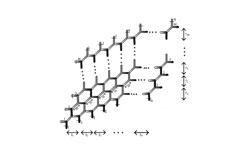
Figure 2: Web diagram of $X_{N,M}$. $t_{i}\in\{t_{1},...,t_{N}\}$ denotes the distance between $i$-th and $i+1$-th lines and $T_{i}\in\{T_{1},...,T_{M}\}$ denotes the distance between $i$-th and $i+1$-th lines. $m$ denotes the Kähler parameter of the diagonal $\mathbb{P}^{1}$s. The double and single bars $|$ and$-$ indicate the periodic identifications.

For example the specific values $M=1,N=k$ correspond to a single M5-brane wrapped on parallel $S^{1}$ and $k$ stack of $M2$-branes wrapped on the transverse $S^{1}$ and ending on the M5-branes. The stack of M2-branes appear as coloured points in the $\mathbb{R}^{4}_{||}$ that resides inside the M5-brane world volume and transverse to the M-string world sheet. Thus for the configuration that involves $n_{l}$ number of M2-branes in the $l$-th stack, where $l=1,...,k$, the moduli space is obviously the product of Hilbert scheme of points as follows

$$\displaystyle\mbox{H}:=\mbox{Hilb}^{n_{1}}[\mathbb{C}^{2}]\times\mbox{Hilb}^{n_{2}}[\mathbb{C}^{2}]\times\cdots\times\mbox{Hilb}^{n_{k}}[\mathbb{C}^{2}]$$ (1.2)

The vector bundle V over H that is required for $(2,0)$ world sheet theory has been determined in Haghighat:2013gba and turns out to be the following

$$\displaystyle V_{I}=\oplus_{t,s=1}^{N}\mbox{Ext}^{1}(\mbox{I}_{r},\mbox{I}_{s})\otimes L^{-\frac{1}{2}}$$ (1.3)

where $\mbox{I}=(\mbox{I}_{1},\mbox{I}_{2},...,\mbox{I}_{N})\in H$. Roughly speaking Ext groups count the massless open string states for strings that are stretched between D-branes wrapped on complex submanifolds of CY spaces. Note that each factor $\mbox{Ext}^{1}(\mbox{I}_{r},\mbox{I}_{s})\otimes L^{-\frac{1}{2}}$ in the fibre denotes the contribution of a pair of stack of M2-branes ending on a single M5-brane from opposite sides. In other words there is an isomorphism between the degrees of freedom on the $(N,M)$ 5-branes web and the moduli space of M-strings, $\mbox{M}(N,\vec{k})$. Using equivariant fixed point theorems one only needs to know the fibres of the bundle $\mbox{V}(N,M)$ over the fixed points.
The weights of $\mbox{V}(N,M)$ at the fixed points $\vec{I}^{(1)},\vec{I}^{(2)},...,\vec{I}^{(M)}$ are given by the following Chern character expansion Hohenegger:2013ala

$$\displaystyle\sum_{weights}e^{w}=\sum_{p=1}^{M}\sum_{r,s=1}^{N}Q_{m}e^{i(a_{r}-a_{s})}\bigg{(}\sum_{(i,j)\in\nu_{r}^{(p)}}t^{\nu_{s,j}^{t,(p+1)}-i+\frac{1}{2}}q^{\nu_{r,i}^{(p)}-j+\frac{1}{2}}+\sum_{(i,j)\in\nu_{s}^{(p+1)}}t^{-\nu_{r,j}^{t,(p)}+i-\frac{1}{2}}q^{-\nu_{s,i}^{(p+1)}+j-\frac{1}{2}}\bigg{)}$$

where $\nu_{1}^{(1)},\nu_{2}^{(1)},...,\nu_{N}^{(1)};\nu_{1}^{(1)},...,\nu_{N}^{(1)}$ label the fixed points. The elliptic genus is then given as follows

$$\displaystyle Z=\int_{M}\prod_{i}\frac{x_{i}\theta_{1}(\tau,\widetilde{x_{i}}+z)}{\theta_{1}(\tau,x_{i})}$$ (1.5)

where $x_{i}$ and $\widetilde{x}_{i}$ denote the Chern roots respectively of the tangent bundle and vector bundle $\mbox{V}(N,M)$ as can be read from (1) and the theta function of first kind $\theta_{1}(\tau,z)$ is defined by

$$\displaystyle\theta_{1}(\tau;z)=-ie^{\frac{i\pi}{4}}(e^{i\pi z}-e^{-i\pi z})\prod_{k=1}^{\infty}(1-e^{2\pi ik\tau})(1-e^{2\pi ik\tau}e^{2\pi ikz})(1-e^{2\pi ik\tau}e^{-2\pi ikz}).$$ (1.6)

More succinctly, the Nekrasov partition function of the gauge theory on the D5-branes of the web is identical to the appropriately normalised topological string partition function of CY threefold $X_{N,M}$ and it is also the generating function of the $(2,0)$ elliptic genus of the product of instanton moduli spaces $\mbox{M}(N,\vec{k})$ on which the bundle $\mbox{V}(N,M)$ coupled to the right moving fermions exists.

Presentation of the paper

We summarised the type IIA/type IIB mirror symmetry conjecture in the introduction (1). In section (3) we construct the quantum mirror curve of $X_{N,M}$ and study the limits in which it can be reduced to a lower genus curve. In section (6) we show that in the splitting degeneration limit the partition function $\mathcal{Z}_{X_{N,M}}$ is recursively related to the partition function $\mathcal{Z}_{X_{N,M-1}}$ and we show this degeneration pictorially. In the appendix we reproduce the proof of an identity used in the main text.

2 (p,q) webs and the mirror curves

We can consider Aganagic:2001nx ; Aganagic:2000gs the A-model topological strings on a toric CY threefold $M=\mathbb{C}^{l+3}//U(1)^{l}$. Algebraically $M$ is defined by the following set of constraints

$$\displaystyle\sum_{i=1}^{l+3}Q_{i}^{a}|X_{i}|^{2}=k^{a},\quad a=1,...,l$$ (2.1)

modulo the action of $U(1)^{l}$, where each $X_{i}$ parameterizes a complex plane $\mathbb{C}$ and can be visualised as $S^{1}$-fibrations over $\mathbb{R}_{+}$. In this way $M$, as defined by (2.1), is a $T^{3}$-fibration over a non-compact convex and linearly bounded subspace in $\mathbb{R}^{3}$, with $T^{3}$ parametrised by $\{\theta_{i}\}$ coordinates. $k^{a}\in\mathbb{R}_{+}$ are called the Kähler parameters. The CY condition

$$\displaystyle c_{1}(TM)=0$$ (2.2)

holds iff

$$\displaystyle\sum_{i=1}^{l+3}Q_{i}^{a}=0,\quad a=1,...,l$$ (2.3)

Inspecting equation (2.1) makes it clear that since $Q_{i}^{a}\in\mathbb{Z}$, all toric CY threefolds are constrained to be non-compact. The second constraint (2.3) furnishes a representation of $M$ as $\mathbb{R}_{+}\times T^{2}$ fibered over $\mathbb{R}^{3}$. In this way the toric threefold M allows its construction by gluing patches of $\mathbb{C}^{3}$.
To construct the mirror N of the threefold M, consider variable $v_{1},v_{2}\in\mathbb{C}$, and the homogeneous coordinates $x_{i}=:e^{y_{i}}\in\mathbb{C}^{*},i=1,...,l+3$ related to $X_{i}$ by $|x_{i}|=e^{-|X_{i}|^{2}}$. The variables $x_{i}$ are constrained by $x_{i}\sim\lambda x_{i}$ for $\lambda\in\mathbb{C}^{*}$. The mirror geometry $N$ is then given by the algebraic equation

$$\displaystyle v_{1}v_{2} = \sum_{i=1}^{l+3}x_{i},$$

subject to the constraints

$$\displaystyle\prod_{i=1}^{l+3}x_{i}^{Q_{i}^{a}} = e^{-r^{a}-i\theta_{a}},\quad a=1,...,l$$ (2.5)

All of these equations can be combined into a single equation

$$\displaystyle v_{1}v_{2}=h(x,y;r^{a},\theta_{a})$$ (2.6)

where $x,y\in\mathbb{C}^{*}$. The function $h(x,y;r^{a},\theta_{a})$ can be decomposed into pant diagrams described by

$$\displaystyle e^{x}+e^{y}+1=0.$$ (2.7)

The last equation describes a conic bundle over $\mathbb{C}^{*}\times\mathbb{C}^{*}$ in which the fibers degenerate over two lines over the family of Riemann surfaces $\Sigma:{g(x,y;r^{a},\theta_{a})=0}\in\mathbb{C}^{*}\times\mathbb{C}^{*}$. If the toric diagram of $M$ is thickened, what emerges is nothing else but $\Sigma$ ; the genus of $\Sigma$ equals the number of closed meshes and the number of punctures equals the number of semi infinite lines in the toric diagram. In the topological A-model the topological vertex computation can be interpreted as the states of a chiral boson on a three-punctured sphere. This chiral boson on each patch of the sphere is identified with the Kodaira Spencer field on the Riemann surface embedded in the CY threefold of mirror topological B-model Huang:2011qx ; Hellerman_2012 ; Gopakumar:1998jq ; Gopakumar:1998ii ; huang2010direct ; katz1997mirror ; Bhardwaj_2016 . The A-model closed topological strings on toric CY threefold, with or without D-branes, is computable by gluing cubic topological vertex expressions. On the mirror B-model the gluing rules are equivalent to the operator formation of the Kodaira Spencer theory on the Riemann surface.The elliptic Calabi-Yau threefold $X_{N,M}$ is dual to the brane web of type IIB $M$ NS5-branes and $N$ D5-branes wrapped on two $\mbox{S}^{1}$s. We denote by $\{y^{0},y^{1},y^{2},y^{3},...,y^{9}\}$ the coordinates of type IIB string theory vacuum $\mathbb{R}^{1,9}$. The common worldvolume of the 5-branes along $\{y^{0},y^{1},y^{2},y^{3},y^{4}\}$ gives rise to the gauge theory under consideration and the $(p,q)$ brane web is arranged in the $\{y^{5},y^{6}\}$ plane which is compactified to a torus $\mbox{T}^{2}$. The $(p,q)$-charges and their conservation encode the details of the five-dimensional mass deformed supersymmetric gauge theory.
The curve associated to a grid diagram is written as the zero locus of a sum of monomials, with each monomial associated to a vertex of the grid diagram. For example $A_{kl}X^{k}Y^{l}$ is a monomial that corresponds to the vertex $(k,l)$. The modulus of the curve $A_{kl}$ is determined by imposing a set of condition: each link on the grid joining e.g. $(k,l)$ to $(u,v)$ uniquely corresponds to a link on the web, which is orthogonal to the former. If the link on the web is given by the line $py=qx+\alpha$, the orthogonality condition is expressed as

$$\displaystyle(k,l)-(u,v)=(-q,p)$$ (2.8)

and the constraint is given by

$$\displaystyle py=qx+\alpha:\quad A_{kl}=e^{\beta\alpha}A_{uv}$$ (2.9)

In other words the mirror curves of toric CY threefolds are determined by the corresponding Newton polygons. The line in the web Aharony_2000 ; nekrasov2002seibergwitten ; Iqbal_2009 ; Aganagic_2004 ; Bershadsky_1996 ; leung1997branes ; Aharony_1998 orthogonal to the line in the Newton polygon joining the coordinates,let’s call them $(k_{1},\ell_{1})$ and $(k_{2},\ell_{2})$ and passing through the point $(x_{0},y_{0})$ is given by ,

$$\displaystyle(\Delta\ell)\,y+(\Delta k)\,x = (\Delta\ell)\,y_{0}+(\Delta k)\,x_{0}$$ (2.10)

where $\Delta\ell=\ell_{2}-\ell_{1}$ and $\Delta k=k_{2}-k_{1}$. Since the choice of $(x_{0},y_{0})$ is arbitrary, we get

$$\displaystyle(\Delta\ell)\,y+(\Delta k)\,x=\alpha$$ (2.11)

The equation of the Riemann surface in this patch is given by exponentiating and complexifying $(x,y)$ to $(u,v)$,

$$\displaystyle X^{\Delta k}\,Y^{\Delta\ell}=-e^{\widetilde{\alpha}}\,,$$ (2.12)

where $X=e^{u}$ and $Y=e^{v}$ with $u,v\in\mathbb{C}$ and $\text{Re}(\widetilde{\alpha})=\alpha$. Since the imaginary part $\widetilde{\alpha}$ is not determined, we have introduced a factor of $-1$ for later convenience. With this choice, $\widetilde{\alpha}$ will be identified with the complexified Kähler parameters. In the mirror curve, we will have

$$\displaystyle A_{k_{1}\ell_{1}}X^{k_{1}}Y^{\ell_{1}}+A_{k_{2}\ell_{2}}X^{k_{2}}Y^{\ell_{2}} = 0$$ (2.13)

which can be solved to give

$$\displaystyle X^{\Delta k}Y^{\Delta\ell}=-\frac{A_{k_{1}\ell_{1}}}{A_{k_{2}}\ell_{2}}~{}~{}~{}~{}~{}~{}~{}\implies~{}~{}~{}~{}~{}A_{k_{2}\ell_{2}}=A_{k_{1}\ell_{1}}\,e^{-\widetilde{\alpha}}$$ (2.14)

3 Mirror curves and their degenerations

We start the discussion by giving an example of Resolved Conifold. In this case, the Newton polygon is shown in figure (3) and the corresponding mirror curve is given by,

$$\displaystyle A_{00}+A_{10}X+A_{01}Y+A_{11}XY=0$$ (3.1)

Let us choose the horizontal line in the web corresponding to the points $(0,0)$ and $(0,1)$ in the Newton polygon that goes through the origin so that $\alpha=0$ for this line. This gives

$$\displaystyle A_{01}=A_{00}$$ (3.2)

Similarly $A_{10}=A_{00}$ and $A_{10}=A_{01}$. The line in the web corresponding to $(0,1),(1,1)$ has the equation $x=T$ where $T$ is the horizontal distance between the two vertices in the web. Note that the vertical distance is also $T$. Thus we get $A_{11}=A_{01}e^{-t}$ where $\text{Re}(t)=T$. The mirror curve is then given by

$$\displaystyle 1+X+Y+e^{2\pi it^{*}}X\,Y=0$$ (3.3)

where $t^{*}=\frac{i}{2\pi}t=\frac{i}{2\pi}T-\frac{\mbox{Im}(t)}{2\pi}$ so that $\mbox{Im}(t^{*})>0$.

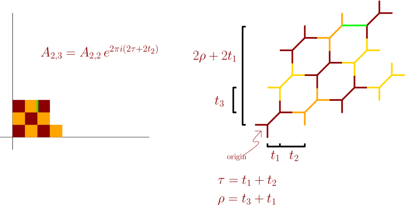
Figure 3: tessellation of Newton polygons and web diagram of $X_{1,1}$

3.1 Mirror curve dual to $X_{1,1}$

Recall that in the mirror construction the Riemann surface $\Sigma$ is a part of the mirror CY threefold. For $6D$ theories the corresponding toric webs have no semi-infinite lines and hence no punctures. The periodicity of the web is taken into account by including all of its images under the periodic shift. Note that after the vertical and horizontal periodic identifications the toric diagram becomes non-planar.
In this case the mirror curve is given by,

$$\displaystyle\sum_{(k,\ell)\in\mathbb{Z}^{2}}A_{k,\ell}X^{k}Y^{\ell}=0\,.$$ (3.4)

Let’s take the origin of the web to be the vertex of the web corresponding to the triangle coordinatized by $(0,0),(1,0),(0,1)$. With this choice the equation of the horizontal line in the web corresponding to $(k,\ell)$ and $(k,\ell+1)$ is given by

$$\displaystyle y=\ell(t_{1}+t_{3})+k\,t_{1}$$ (3.5)

where $\tau$ is the periodicity of the web in the vertical direction and $t_{1}$ is the horizontal distance between two consecutive vertices on the diagonal in the web given in figure (3). This gives

$$\displaystyle A_{k,\ell+1}=A_{k,\ell}e^{2\pi i(\ell\tau+k\,z)}\implies A_{k,\ell+1}=A_{k,0}e^{2\pi i(\tau\frac{\ell(\ell+1)}{2}+(\ell+1)k\,z)}$$ (3.6)

where $\mbox{Im}(\tau)=\frac{t_{1}+t_{3}}{2\pi}$ and $\mbox{Im}(z)=\frac{t_{1}}{2\pi}$. The equation of the line in the web corresponding to $(k,\ell),(k+1,\ell)$ is given by $x=k(t_{1}+t_{2})+\ell t_{1}$ where $\rho$ is the periodicity of the web in the horizontal direction. We thus get

$$\displaystyle A_{k+1,\ell}=A_{k,\ell}e^{2\pi i(k\rho+\ell z)}\implies A_{k+1,\ell}=A_{0,\ell}e^{2\pi i(\rho\frac{k(k+1)}{2}+(k+1)\ell z)}$$ (3.7)

From Eq.(3.6) and Eq.(3.7) it follows that

$$\displaystyle A_{k,\ell}=A_{0,0}e^{2\pi i(\frac{\ell(\ell-1)}{2}\tau+\frac{k(k-1)}{2}\rho+\ell kz)}$$ (3.8)

Using the coefficients the mirror curve becomes

$$\displaystyle\sum_{k,\ell\in\mathbb{Z}}e^{2\pi i(\frac{\ell(\ell-1)}{2}\tau+\frac{k(k-1)}{2}\rho+\ell kz)}X^{k}Y^{\ell}=0$$ (3.9)

If we define the genus two theta function by

$$\displaystyle\Theta\Big{(}\Omega(\rho,z,\tau)|(u,v)\Big{)}=\sum_{k,\ell}\mbox{exp}\Big{(}2\pi iQ(k,\ell)/2\Big{)}X^{k}Y^{\ell}$$ (3.10)

where the period matrix $\Omega(\rho,z,\tau)$ and the quadratic form $Q(k,.)$ are given by

$$\displaystyle\Omega(\rho,z,\tau):=\left(\begin{array}[]{cc}\rho&z\\ z&\tau\\ \end{array}\right)\,,\,\,\,\,\,Q(k,\ell):=(k\,\,\ell)\Omega(\rho,z,\tau)\left(\begin{array}[]{c}k\\ \ell\\ \end{array}\right)$$ (3.15)

the mirror curve can be written as

$$\displaystyle\Theta\Big{(}\Omega(\rho,z,\tau)|(u,v)\Big{)}=0$$ (3.16)

It is interesting to note Hollowood_2008 ; Haghighat_2019 that under the following identifications

$$\displaystyle X\to Xe^{2\pi i\tau}, \quad Y\to Ye^{z}$$

$$Y\to Y^{2\pi i\rho}, \quad X\to Xe^{z}$$ (3.17)

the theta function transforms covariantly and the curve (3.16) remains invariant . Note that in the limit $z\to 0$ the left side is factorized into the product of genus one theta functions

$$\displaystyle\big{(}\sum_{k,\in\mathbb{Z}}e^{2\pi i(\frac{k(k-1)}{2}\rho)}X^{k}\big{)}\big{(}\sum_{\ell\in\mathbb{Z}}e^{2\pi i(\frac{\ell(\ell-1)}{2}\tau)}Y^{\ell}\big{)}=0$$ (3.31)

3.2 Mirror curve dual to $X_{1,2}$

Consider the periodic Newton polygon with vertices $(0,0),(1,0),(2,0),(2,1),(1,1),(0,1)$ as shown in figure (4). The mirror curve is given by

$$\displaystyle\sum_{k,\ell\in\mathbb{Z}}B_{k\ell}\,X^{k}Y^{\ell}=0$$ (3.32)

where the coefficients $B_{k,\ell}$ can be determined in the same way as for the genus two case and are functions of the four Kähler parameters $(\tau,\rho,z,w)$.

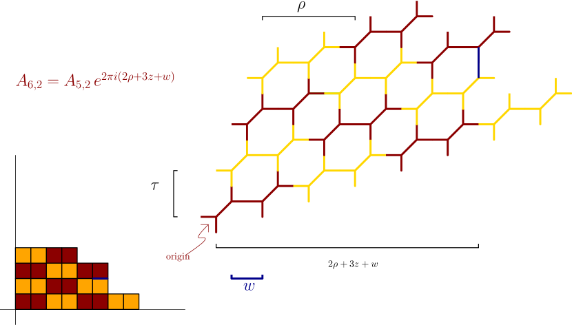
Figure 4: tessellation of Newton polygons and web diagram of $X_{1,2}$

They are related to each other as follows:

$$\displaystyle B_{2k+2,\ell}=B_{2k+1,\ell}e^{2\pi i(k\rho+(\ell+1)z+w)}\,,\,\,\,B_{2k+1}=B_{2k,\ell}e^{2\pi i(k\rho+\ell z)},\,\,\,B_{k,\ell+1}=B_{k,\ell}e^{2\pi i(\ell\,\tau+k\,z)}$$ (3.33)

These recursive relations have the following solution:

$$\displaystyle B_{2k,\ell} = \mbox{exp}\Big{[}2\pi i\Big{(}k(k-1)\rho+\frac{\ell(\ell-1)}{2}\tau+2k\ell z+kz+kw\Big{)}\Big{]}$$

$$B_{2k+1,\ell} = \mbox{exp}\Big{[}2\pi i\Big{(}k^{2}\rho+\frac{\ell(\ell-1)}{2}\tau+(2k+1)\ell z+k(z+w)\Big{)}\Big{]}$$

Then the mirror curve is given by

$$\displaystyle\Theta\Big{(}\Omega(2\rho,2z,\tau)|(2u-\rho+z+w,v-\tau)\Big{)}+e^{2\pi iu}\Theta\Big{(}\Omega(2\rho,2z,\tau)|(2u+z+w,v-\tau+z)\Big{)}=0$$

To see the factorisation we can write the last expression explicitly as

$$\displaystyle\sum_{k,\ell\in\mathbb{Z}}\bigg{(}\mbox{exp}\Big{[}2\pi i\Big{(} k(k-1)\rho+\frac{\ell(\ell-1)}{2}\tau+2k\ell z+kz+kw\Big{)}\Big{]}X^{2k}Y^{\ell}$$

$$+ \mbox{exp}\Big{[}2\pi i\Big{(}k^{2}\rho+\frac{\ell(\ell-1)}{2}\tau+(2k+1)\ell z+k(z+w)\Big{)}\Big{]}X^{2k+1}Y^{\ell}\bigg{)}=0$$ (3.35)

It is easy to see that In the limit $z\to 0$ we get the factorized form

$$\displaystyle\bigg{(}\sum_{\ell\in\mathbb{Z}}\mbox{exp}\Big{[}2\pi i\Big{(}\frac{\ell(\ell-1)}{2}\tau\Big{)}\Big{]}Y^{\ell}\bigg{)}\bigg{(}\sum_{k\in\mathbb{Z}}X^{2k}\bigg{(} \mbox{exp}\Big{[}2\pi i\Big{(}k(k-1)\rho+kw\Big{)}\Big{]}+\mbox{exp}\Big{[}2\pi i\Big{(}k^{2}\rho+kw\Big{)}\Big{]}X\bigg{)}\bigg{)}=0$$

3.3 Mirror curve dual to $X_{N,M}$

Figure 5: Web diagram of $X_{N,M}$. $t_{i}\in\{t_{1},...,t_{N}\}$ denotes the distance between $i$-th and $i+1$-th vertical lines and $T_{i}\in\{T_{1},...,T_{M}\}$ denotes the distance between $i$-th and $i+1$-th horizotntal lines. $\bf{m}_{a,b}$ parametrize the diagonal $\mathbb{P}^{1}$s.

Consider the $(N,M)$ web shown in figure (5). The Kähler class $\omega$ of $X_{N,M}$ is parameterized by $(m_{\alpha,\beta},\tau,\rho,{\bf T},{\bf t})=(m_{\alpha,\beta},\tau,\rho,m,T_{1},T_{2},\cdots,T_{M-1},t_{1},t_{2},\cdots,t_{N-1})$ with $\tau=\sum_{i=1}^{M}T_{i}$ and $\rho=\sum_{j=1}^{N}t_{j}$. For arbitrary $(N,M)$ values the factorisation properties of the mirror curve will in general be affected by the quantum corrections. The quantum corrected Kähler parameters are the solutions of the Picard-Fuchs equations Iqbal:2001kk . After getting quantum corrections various Kähler parameters are mixed non-trivially and that renders the factorisation non-trivial as compared to the classical case discussed here.
The mirror curve is given by a sum over the monomials associated with the Newton polygon. In this case the Newton polygon tiles the plane

$$\displaystyle H_{N,M}(X,Y):=\sum_{(i,j)\in\mathbb{Z}^{2}}A_{i,j}X^{i}\,Y^{j}\,.$$ (3.37)

The coefficients $A_{i,j}$ depend on the length of the various line segments in the web which are the Kähler parameters of the corresponding Calabi-Yau threefolds. As discussed before the neighbouring pair of points in the Newton polygon connected by a line give a relation between the associated coefficients $A_{i,j}$,

$$\displaystyle\frac{A_{i,k+1}}{A_{i,k}}=e^{\sum_{j=1}^{k-1}T_{j}+\sum_{\alpha=0}^{i-1}m_{\alpha,k}}$$ (3.38)

$$\frac{A_{i+1,k}}{A_{i,k}}=e^{\sum_{j=1}^{i-1}t_{j}+\sum_{\alpha=0}^{k-1}m_{i,\alpha}}$$

$$\displaystyle A_{i+1,k+1} = A_{i+1,1}e^{T_{1}+(T_{1}+T_{2})+(T_{1}+T_{2}+T_{3})+\cdots+(T_{1}+\cdots+T_{k-1})+\sum_{\beta=1}^{k}\sum_{\alpha=0}^{i}m_{\alpha,\beta}}$$

$$= A_{i+1,1}e^{\sum_{\gamma=1}^{k-1}(k-\gamma)T_{\gamma}+\sum_{\beta=1}^{k}\sum_{\alpha=0}^{i}m_{\alpha,\beta}}$$

$$= A_{0,1}e^{t_{1}+(t_{1}+t_{2})+\cdots+(t_{1}+t_{2}+\cdots+t_{i-1})}e^{\sum_{\gamma=1}^{k-1}(k-\gamma)T_{\gamma}+\sum_{\beta=0}^{k}\sum_{\alpha=0}^{i}m_{\alpha,\beta}}$$

where in the web diagram of $X_{N,M}$, $t_{i}\in\{t_{1},...,t_{N}\}$ denotes the distance between $i$-th and $i+1$-th vertical lines and $T_{i}\in\{T_{1},...,T_{M}\}$ denotes the distance between $i$-th and $i+1$-th horizotntal lines and $\bf{m}_{a,b}$ parametrize the diagonal finite line segments representing $\mathbb{P}^{1}$s.
Using $A_{0,1}=A_{0,0}=1$ we get the following solution

$$\displaystyle A_{i+1,k+1} = e^{\sum_{\gamma=1}^{i-1}(i-\gamma)t_{\gamma}+\sum_{\gamma=1}^{k-1}(k-\gamma)T_{\gamma}+\sum_{\beta=0}^{k}\sum_{\alpha=0}^{i}m_{\alpha,\beta}}$$ (3.40)

Thus the curve is given by

$$\displaystyle H_{N,M}(X,Y) = \sum_{(i,k)\in\mathbb{Z}^{2}}A_{i+1,k+1}X^{i+1}Y^{k+1}$$

$$= \sum_{i=0,k=0}^{N-1,M-1}W_{i,k}(X,Y)$$

$$W_{i,k}(X,Y) = \sum_{(a,b)\in\mathbb{Z}^{2}}A_{Na+i+1,Mb+k+1}X^{Na+i+1}Y^{Mb+k+1}$$

$$\displaystyle A_{Na+i+1,Mb+k+1}=e^{\sum_{\gamma=1}^{Na+i-1}(Na+i-\gamma)t_{\gamma}+\sum_{\gamma=1}^{Mb+k-1}(Mb+k-\gamma)T_{\gamma}+\sum_{\beta=0}^{Mb+k}\sum_{\alpha=0}^{Na+i}m_{\alpha,\beta}}$$ (3.42)

Using the identifications

$$\displaystyle t_{\gamma} = t_{\gamma^{\prime}}\,\,\,\,\mbox{if}\,\,\,\,\,\gamma\equiv\gamma^{\prime}\,(\mbox{mod}\,N)$$ (3.43)

$$T_{\gamma} = T_{\gamma^{\prime}}\,\,\,\,\mbox{if}\,\,\,\,\,\gamma\equiv\gamma^{\prime}\,(\mbox{mod}\,M)$$

$$m_{\alpha_{1},\beta_{1}} = m_{\alpha_{2},\beta_{2}}\,\,\,\,\,\mbox{if}\,\,\,\,\,\,\,\alpha_{1}\equiv\alpha_{2}\,(\mbox{mod}\,N)\,\,\,\mbox{and}\,\,\,\,\beta_{1}\equiv\beta_{2}\,(\mbox{mod}\,M)$$

we get

$$\displaystyle\sum_{\gamma=1}^{Na+i-1}(Na+i-\gamma)t_{\gamma} = \sum_{\gamma=1}^{N}(Na+i-\gamma)t_{\gamma}+\sum_{\gamma=N+1}^{2N}(Na+i-\gamma)t_{\gamma}+\cdots$$

$$+\sum_{\gamma=N(a-1)+1}^{Na}(Na+i-\gamma)t_{\gamma}+\sum_{\gamma=Na+1}^{Na+i-1}(Na+i-\gamma)t_{\gamma}$$

$$= \sum_{\gamma=1}^{N}\Big{[}(Na+i-\gamma)+(N(a-1)+i-\gamma)+(N(a-2)+i-\gamma)+\cdots+$$

$$(N+i-\gamma)\Big{]}t_{\gamma}+\sum_{\gamma=1}^{i-1}(i-\gamma)t_{\gamma}$$

$$= \sum_{\gamma=1}^{N}\Big{[}N\tfrac{a(a+1)}{2}+a(i-\gamma)\Big{]}t_{\gamma}+\sum_{\gamma=1}^{i-1}(i-\gamma)t_{\gamma}$$

$$= \Big{[}N\tfrac{a(a+1)}{2}+ai\Big{]}\tau-\sum_{\gamma=1}^{N}\gamma\,t_{\gamma}+\sum_{\gamma=1}^{i-1}(i-\gamma)t_{\gamma}$$

Similarly

$$\displaystyle\sum_{\gamma=1}^{Mb+k-1}(Mb+k-\gamma)T_{\gamma}=\Big{[}M\tfrac{b(b+1)}{2}+bk\Big{]}\rho-\sum_{\gamma=1}^{M}\gamma\,T_{\gamma}+\sum_{\gamma=1}^{k-1}(k-\gamma)T_{\gamma}$$ (3.45)

$$\displaystyle\sum_{\beta=0}^{Mb+k}\sum_{\alpha=0}^{Na+i}m_{\alpha,\beta} = \sum_{\beta=0}^{Mb+k}\Big{[}\sum_{\alpha=0}^{N-1}m_{\alpha,\beta}+\sum_{\alpha=N}^{2N-1}m_{\alpha,\beta}+\cdots+\sum_{\alpha=N(a-1)}^{Na-1}m_{\alpha,\beta}+\sum_{\alpha=Na}^{Na+i}m_{\alpha,\beta}\Big{]}$$

$$= \sum_{\beta=0}^{Mb+k}\Big{[}a\sum_{\alpha=0}^{N-1}m_{\alpha,\beta}+\sum_{\alpha=0}^{i}m_{\alpha,\beta}\Big{]}$$

$$= a\sum_{\alpha=0}^{N-1}\Big{[}b\sum_{\beta=0}^{M-1}m_{\alpha,\beta}+\sum_{\beta=0}^{k}m_{\alpha,\beta}\Big{]}+\sum_{\alpha=0}^{i}\Big{[}b\sum_{\beta=0}^{M-1}m_{\alpha,\beta}+\sum_{\beta=0}^{k}m_{\alpha,\beta}\Big{]}$$

$$= ab\sum_{\alpha=0}^{N-1}\sum_{\beta=0}^{M-1}m_{\alpha,\beta}+a\sum_{\alpha=0}^{N-1}\sum_{\beta=0}^{k}m_{\alpha,\beta}+b\sum_{\alpha=0}^{i}\sum_{\beta=0}^{M-1}m_{\alpha,\beta}+\sum_{\alpha=0}^{i}\sum_{\beta=0}^{k}m_{\alpha,\beta}$$

Since $\sum_{\alpha=0}^{N-1}m_{\alpha,\beta}$ is independent of $\beta$ by Lemma 5.4 of Kanazawa:2016tnt therefore

$$\displaystyle\sum_{\beta=0}^{Mb+k}\sum_{\alpha=0}^{Na+i}m_{\alpha,\beta} = (ab+\tfrac{a(k+1)}{M}+\tfrac{b(i+1)}{N})\sum_{\alpha=0}^{N-1}\sum_{\beta=0}^{M-1}m_{\alpha,\beta}+\sum_{\alpha=0}^{i}\sum_{\beta=0}^{k}m_{\alpha,\beta}$$

$$= (ab+\tfrac{a(k+1)}{M}+\tfrac{b(i+1)}{N}){\bf m}+{\bf m}^{i,k}$$

$$\sum_{\gamma=1}^{Na+i-1}(Na+i-\gamma)t_{\gamma}+\sum_{\gamma=1}^{Mb+k-1}(Mb+k-\gamma)T_{\gamma}+\sum_{\beta=0}^{Mb+k}\sum_{\alpha=0}^{Na+i}m_{\alpha,\beta}+$$

$$z_{1}(Na+i+1)+z_{2}(Mb+k+1)=$$

$$\Big{[}N\tfrac{a(a+1)}{2}+ai\Big{]}\tau-\sum_{\gamma=1}^{N}\gamma\,t_{\gamma}+\sum_{\gamma=1}^{i-1}(i-\gamma)t_{\gamma}+\Big{[}M\tfrac{b(b+1)}{2}+bk\Big{]}\rho-\sum_{\gamma=1}^{M}\gamma\,T_{\gamma}+\sum_{\gamma=1}^{k-1}(k-\gamma)T_{\gamma}+$$

$$(ab+\tfrac{a(k+1)}{M}+\tfrac{b(i+1)}{N}){\bf m}+{\bf m}^{i,k}+z_{1}(Na+i+1)+z_{2}(Mb+k+1)$$

$$= G^{i,k}_{N,M}({\bf t},{\bf T},{\bf m})+\tfrac{1}{2}(a+\tfrac{i+1}{N},b+\tfrac{k+1}{M})\begin{pmatrix}N\tau&{\bf m}\\ {\bf m}&M\rho\end{pmatrix}\begin{pmatrix}a+\tfrac{i+1}{N}\\ b+\tfrac{k+1}{M}\end{pmatrix}+a\tau(\tfrac{N}{2}-1)+b\rho(\tfrac{M}{2}-1)$$

$$-\tfrac{(i+1)(k+1)}{MN}{\bf m}-\tfrac{1}{2}(\tfrac{i+1}{N})^{2}\,N\tau-\tfrac{1}{2}(\tfrac{k+1}{M})^{2}\,M\rho+Nz_{1}(a+\tfrac{i+1}{N})+Mz_{2}(b+\tfrac{k+1}{M})$$

$$= G^{i,k}_{N,M}({\bf t},{\bf T},{\bf m})+\tfrac{1}{2}({\bf n}+{\bf u})^{t}\Omega({\bf n}+{\bf u})+({\bf n}+{\bf u})\cdot(\widehat{\bf z}+{\bf v})$$

where

$$\displaystyle G^{i,k}_{N,M}({\bf t},{\bf T},{\bf m}) = -\tfrac{(k+1)(M+k-1)}{2M}\rho-\tfrac{(i+1)(N+i-1)}{2N}\tau+{\bf m}^{i,k}-\sum_{\gamma=1}^{N}\gamma\,t_{\gamma}+\sum_{\gamma=1}^{i-1}(i-\gamma)t_{\gamma}$$ (3.49)

$$-\sum_{\gamma=1}^{M}\gamma\,T_{\gamma}+\sum_{\gamma=1}^{k-1}(k-\gamma)T_{\gamma}$$

$$\widehat{\bf z} = (Nz_{1},Mz_{2})$$

$${\bf u} = (\tfrac{i+1}{N},\tfrac{k+1}{M})$$

$${\bf v} = (\tau(\tfrac{N}{2}-1),\rho(\tfrac{M}{2}-1))$$

We define the genus two theta function as:

$$\displaystyle\Theta_{\vec{u},\vec{v}}(\vec{z},\Omega)=\sum_{\vec{n}\in\mathbb{Z}^{2}}e^{\frac{1}{2}(\vec{n}+\vec{u})^{t}\Omega(\vec{n}+\vec{u})+(\vec{n}+\vec{u})\cdot(\vec{z}+\vec{v})}$$ (3.50)

Then

$$\displaystyle W^{i,k}(X,Y)=\sum_{(a,b)\in\mathbb{Z}^{2}}e^{G^{i,k}_{N,M}}\,\Theta_{\vec{u},\vec{v}}(\vec{z},\Omega)$$ (3.51)

The genus of the mirror curve

$$\displaystyle\sum_{i=0,k=0}^{N-1,M-1}W_{i,k}(X,Y)=0$$ (3.52)

is $MN+1$. The underlying abelian surface has polarisation $(N,M)$ with the period matrix given by $\Omega=\begin{pmatrix}N\tau&{\bf m}\\ {\bf m}&M\rho\end{pmatrix}$. The theta functions form a basis corresponding to this $(N,M)$-polarization of the abelian surface.

3.4 Geometric interpretation of the mirror curve

An illuminative way to visualise the mirror curve $\Sigma$ is to see it as N copies of the base torus glued together by N-1 branch cuts Braden:2003gv ; Hollowood_2008 . The one cycles, A and B, of the base torus are lifted to a basis of 1-cycles $A_{i},B_{i},i=1,...,N$ on $\Sigma$. Riemann-Hurwitz theorem is used to compute the genus of $\Sigma$ and is equal to N+1. The Riemann-Roch theorem is handy in the computation of the number of moduli of $\Sigma$, which is equal to N in this case.
In the case under consideration, the genus N Riemann surface is seen as defined by theta divisor. A general polarised abelian variety $\mathcal{U}$ admits a line bundle $\mathcal{L}$ with $c_{1}(\mathcal{L})=\omega$ where $\omega$ is a $(1,1)$-form that is given in terms of the coordinates $0\leq y_{i}\leq 1$ by

$$\displaystyle\omega=[Ndy_{1}\wedge dy_{3}+dy_{2}\wedge dy_{4}]$$ (3.53)

where it is assumed that the period matrix $\Omega$ of $\Sigma$ is symmetric and $Im(\Omega)>0$. For general abelian variety with polarisation given by $\omega=[Ndy_{1}\wedge dy_{3}+Mdy_{2}\wedge dy_{4}]$ the line bundle $\mathcal{L}$ admits $MN$ holomorphic sections. In the case of an abelian surface these sections are given by genus $2$ theta functions

$$\displaystyle\Theta\left[{\begin{array}[]{cc}\frac{i}{M}&\frac{j}{N}\\ 0&0\\ \end{array}}\right](z|\Omega)\quad 0\leq i<M,\quad 0\leq j<N.$$ (3.56)

A theta divisor is the zero locus of a linear combination of the above set of theta functions

$$\displaystyle\sum_{i}^{M}\sum_{j}^{N}A_{ij}\Theta\left[{\begin{array}[]{cc}\frac{i}{M}&\frac{j}{N}\\ 0&0\\ \end{array}}\right](\vec{z}|\Omega)=0$$ (3.59)

where $A_{ij}$ denote the moduli of the curve. This zero locus defines the mirror curve of genus $MN+1$ and is the Riemann surface $\Sigma$. For the special case of $M=1$ the mirror curve can be expressed in the following form

$$\displaystyle\sum_{n=0}\frac{1}{n!}(\frac{m}{2\pi i})^{n}\partial_{z}^{n}\theta_{1}(z|\tau)\partial_{x}^{n}h(x)=0$$ (3.60)

where $\theta_{1}$ is the Jacobi theta function and $h(x)=\prod_{j=1}^{N}\theta_{1}(x-\xi_{j}|\rho)$ with $\xi_{j}$ is the moduli of $\Sigma$. This can be reorganised into the following form

$$\displaystyle\Theta_{[\frac{1}{2},...,\frac{1}{2}],[\frac{1}{2},...,\frac{1}{2}]}(z,\frac{N\beta}{2\pi}(x-\xi_{i})|\hat{\Omega})=0$$ (3.61)

where $\hat{\Omega}$ is the period matrix of the genus MN+1 curve $\hat{\Sigma}$ which is an unbranched cover of a genus 2 curve and in general is given by

$$\displaystyle\hat{\Omega}=\left[{\begin{array}[]{ccccc}\tau&\frac{\beta m_{1}}{2\pi i}&\frac{\beta m_{2}}{2\pi i}&\frac{\beta m_{3}}{2\pi i}&...\frac{\beta m_{MN}}{2\pi i}\\ \frac{\beta m_{1}}{2\pi i}&\rho&0&0&...0\\ \frac{\beta m_{2}}{2\pi i}&0&\rho&0&...0\\ .&.&.&.&\\ .&.&.&.&\\ .&.&.&.&\\ \frac{\beta m_{MN}}{2\pi i}&0&0&0&...\rho\\ \end{array}}\right]$$ (3.69)

It is easy to see from the following representation of genus $g=MN+1$ theta function

$$\displaystyle\Theta\left[{\begin{array}[]{c}\alpha\\ \beta\end{array}}\right](Z|\hat{\Omega})=\sum_{m\in\mathbb{Z}^{g}}exp\bigg{(}\pi i(m+\alpha).\hat{\Omega}.(m+\alpha)+2\pi i(Z+\beta).(m+\alpha)\bigg{)}$$ (3.72)

where $Z,\alpha,\beta,m$ are g-vectors and $\Omega$ is a $g\times g$ matrix with $Im\Omega>0$.
To study the decomposition of generalised theta function Marshakov:1999bw defined on the Jacobian of a genus $g=M$ curve, we start from the following Fourier representation

$$\displaystyle\Theta(\Omega|\vec{z})=\sum_{\textbf{m}\in\mathbb{Z}^{M}}e^{2\pi i\sum_{i=1}^{M}m_{i}z_{i}+i\pi\sum_{i,j=1}^{M}m_{i}\Omega_{ij}m_{j}}$$ (3.73)

where $\Omega$ is the period matrix and satisfies the following constraints

$$\displaystyle\sum_{i=1}^{M}\Omega_{ij} = \tau,\quad\sum_{j=1}^{M}\Omega_{ij}=\tau$$ (3.74)

This constraint encodes various periodicity properties. In other words we can decompose $\Omega$ as

$$\displaystyle\Omega=\frac{\tau}{M}+\Omega^{\prime}$$ (3.75)

where $\Omega^{\prime}$ is the traceless part. Now redefine $z_{i}$ as follows

$$\displaystyle z_{i} = \frac{z}{M}+z_{i}^{\prime}\quad\mbox{such that}\quad\sum_{i=1}^{M}z_{i}^{\prime}=0$$ (3.76)

Putting back these redefined variables in (3.73) we get

$$\displaystyle\Theta(\Omega|\vec{z}) = \sum_{\textbf{m}\in\mathbb{Z}^{M}}e^{2\pi i\frac{z}{M}\sum_{i=1}^{M}m_{i}+i\pi\frac{\tau}{M}(\sum_{i=1}^{M}m_{i})^{2}+2\pi i\sum_{i=1}^{M}m_{i}z_{i}^{\prime}+\pi i\sum_{i,j=1}^{M}m_{i}\Omega^{\prime}_{ij}m_{i}}$$ (3.79)

$$= \sum_{i\in\mathbb{Z}_{M},s\in\mathbb{Z}}e^{2\pi i(s+\frac{i}{M})z+\pi i\tau M(s+\frac{i}{M})^{2}}\sum_{\textbf{m}\in\mathbb{Z}^{M},\sum_{j=1}^{M}m_{j}=i}e^{i2\pi\sum_{p=1}^{M}m_{p}z_{p}^{\prime}+\pi i\sum_{p,q=1}^{M}m_{p}\Omega^{\prime}_{pq}m_{q}}$$

$$= \sum_{i\in\mathbb{Z}_{M}}\theta\left[{\begin{array}[]{c}\frac{i}{M}\\ 0\end{array}}\right](M\tau|z)\Theta_{i}(\Omega^{\prime}|\vec{z}^{\prime})$$

where $\Theta_{i}$ is the second summation factor in the first line of (3.79).

4 Degenerations and their Effect on the Partition Function

The partition function of the CY threefold $X_{N,M}$ is given by Hohenegger:2013ala

$$\displaystyle\mathcal{Z}_{(N,M)}(\tau,\rho,\epsilon_{1,2},m_{a}=m,t) =\sum_{\alpha_{a}^{i}}\,\prod_{i=1}^{N}Q_{i}^{|\alpha^{(i)}|}\,\prod_{i=1}^{N}\prod_{a=1}^{M}\,\frac{\vartheta_{\alpha_{a}^{i+1}\alpha_{a}^{i}}(m)}{\vartheta_{\alpha_{a}^{i}\alpha_{a}^{i}}(\epsilon_{+})}$$ (4.1)

$$\prod_{1\leq a<b\leq M}\prod_{i=1}^{N}\frac{\vartheta_{\alpha_{a}^{i}\alpha_{b}^{i+1}}(t_{ab}-m)\vartheta_{\alpha_{a}^{i+1}\alpha_{b}^{i}}(t_{ab}+m)}{\vartheta_{\alpha_{a}^{i}\alpha_{b}^{i}}(t_{ab}-\epsilon_{+})\vartheta_{\alpha_{a}^{i}\alpha_{b}^{i}}(t_{ab}+\epsilon_{+})}$$

where the sum is over $N$ partitions of $\alpha^{(a)}=\{\alpha_{1}^{(a)},\alpha_{2}^{(a)},...,\alpha_{N}^{(a)}\}$ and $\alpha_{a}^{(1)}\equiv\alpha_{a}^{(N+1)}$, $Q_{i}=e^{b_{i+1}-b_{i}}$, $t_{ab}=t_{a,a+1}+t_{a+1,a+2}+\cdots+t_{a+b-(a+1),b}$, $b_{i+1}-b_{i}$ is the distance between vertical lines (or M5 branes) and moreover the factorisation degeneration takes place when all the mass parameters $m_{a}$ are taken equal to $m$. The expressions of partition functions after degeneration becomes particularly simple at the special point in the Kähler moduli space where $Q_{i}:=Q:=e^{2\pi i\tau}$ and in the unrefined limit of the $\Omega$-background parameters $\epsilon_{1}=-\epsilon_{2}=\epsilon$.

We define

$$\displaystyle|\alpha^{(a)}|=\sum_{b=1}^{N}|\alpha_{b}^{(a)}|$$ (4.2)

where $|\alpha^{(a)}|$ is the size of the partition $\alpha^{(a)}$ which is the sum of the parts of partition. To study the degeneration of partition function we have to study the $x\to 0$ limit of $\vartheta_{\mu\nu}(x)$. For two integer partitions $\mu$ and $\nu$, theta function $\vartheta_{\mu\nu}$ in the above partition function (4.1) is defined as

$$\vartheta_{\mu\nu}(x)=\prod_{(i,j)\in\mu}\vartheta(\rho,e^{-x}\,t^{-\nu^{t}_{j}+i-\tfrac{1}{2}}\,q^{-\mu_{i}+j-\tfrac{1}{2}})\,\prod_{(i,j)\in\nu}\vartheta(\rho,e^{-x}\,t^{\mu^{t}_{j}-i+\tfrac{1}{2}}\,q^{\nu_{i}-j+\tfrac{1}{2}})\,$$ (4.3)

Here $t=e^{-i\epsilon_{2}},q=e^{i\epsilon_{1}}$, $\nu^{t}$ represents the transpose of the partition $\nu$ and product $\prod\limits_{(i,j)\in\nu}$ means that the product is over all the boxes of the Young diagram corresponding to the partition $\nu$ having length $\ell(\nu)$

$$(i,j)\in\nu\,,\quad\textrm{implies that}\quad 1\leq i\leq\ell(\nu),\quad 1\leq j\leq\nu_{i}.$$

The Jacobi theta function $\vartheta(\rho,y)$ for $y=e^{2\pi iz}$ is defined as

$$\displaystyle\vartheta(\rho,y)=(y^{\tfrac{1}{2}}-y^{-\tfrac{1}{2}})\prod_{k=1}^{\infty}(1-y\,e^{2\pi ik\rho})(1-y^{-1}\,e^{-2\pi ik\rho})$$

For $x=0$ and in unrefined case

$$\displaystyle\vartheta_{\mu\nu}(0) =-\prod_{(i,j)\in\mu}\vartheta(\rho,\nu^{t}_{j}-i+\mu_{i}-j+1)\,\prod_{(i,j)\in\nu}\vartheta(\rho,\mu^{t}_{j}-i+\nu_{i}-j+1)$$ (4.4)

$$=-\prod_{(i,j)\in\mu}\vartheta(\rho,h_{\mu}(i,j)+\nu^{t}_{j}-\mu^{t}_{j})\,\prod_{(i,j)\in\nu}\vartheta(\rho,h_{\nu}(i,j)+\mu^{t}_{j}-\nu^{t}_{j})\,$$

where $h_{\mu}(i,j)=\mu_{i}+\mu_{j}^{t}-i-j+1$ is the hook length of the partition $\mu$. Since, the Jacobi theta function $\vartheta(\rho,z)$ is an odd function w.r.t. $z$ i.e., $\vartheta(\rho,0)=0$, therefore $\vartheta_{\mu\nu}(0)=0$ if $h_{\mu}(i,j)+\nu^{t}_{j}-\mu^{t}_{j}=0$. Since $h_{\mu}(i,j)\neq 0$, therefore $\nu^{t}_{j}\neq\mu^{t}_{j}$. If $\mu=\nu$ then

$$\displaystyle\vartheta_{\mu\mu}(0)=\prod_{(i,j)\in\mu}\vartheta(\rho,h_{\mu}(i,j))^{2}$$

$h_{\mu}(i,j)$ is non zero therefore $\vartheta_{\mu\mu}(0)\neq 0.$ In other words $\mu\neq\nu$ implies $\vartheta_{\mu\nu}(0)=0$ i.e. either $h_{\mu}(i,j)+\nu^{t}_{j}-\mu^{t}_{j}=0$ or $h_{\nu}(i,j)+\mu^{t}_{j}-\nu^{t}_{j}=0.$ Because $h_{\mu}(i,j)\neq 0$ therefore $\nu^{t}_{j}\neq\mu^{t}_{j}$. We thus arrive at the useful property of $\vartheta_{\mu\nu}(x)$ at $x=0$ given by:

$$\displaystyle\vartheta_{\mu\nu}(0)=\delta_{\mu\,\nu}\,\prod_{(i,j)\in\mu}\vartheta(q^{h_{\mu}(i,j)})\vartheta(q^{-h_{\mu}(i,j)})$$ (4.5)

where $\delta_{\mu\,\nu}$ is the kronecker delta function and $h_{\mu}(i,j)=\mu_{i}+\mu_{j}^{t}-i-j+1$ is the hook length of the partition $\mu$. This identity is useful for studying different degenerations of the partition functions.

5 Degeneration 1:Factorization

This type of degeneration corresponds to taking both the vertical and horizontal ‘distances’ between the 5-branes equal to $m$, which is the Kähler parameter corresponding to the exceptional curve or $(1,1)$ brane in the web diagram fig.5.

5.1 $(N,M)=(1,2)$

We begin by looking at the case of $X_{1,2}$. The unrefined partition function is given by,

$$\displaystyle\mathcal{Z}_{(1,2)}(\tau,\rho,m,t,\epsilon) = \sum_{\alpha_{1,2}}\,Q^{|\alpha_{1}|+|\alpha_{2}|}\,\frac{\vartheta_{\alpha_{1}\alpha_{1}}(m)\vartheta_{\alpha_{2}\alpha_{2}}(m)}{\vartheta_{\alpha_{1}\alpha_{1}}(0)\vartheta_{\alpha_{2}\alpha_{2}}(0)}\frac{\vartheta_{\alpha_{1}\alpha_{2}}(t^{-}_{m})\vartheta_{\alpha_{1}\alpha_{2}}(t^{+}_{m})}{\vartheta_{\alpha_{1}\alpha_{2}}(t)^{2}}$$ (5.1)

Here, $t^{-}_{m}=t-m$ and $t^{+}_{m}=t+m$. The partition function $Z_{(1,2)}$ in the limit $t\mapsto m$ reduces to

$$\displaystyle\mathcal{Z}_{(1,2)}(\tau,\rho,m,\epsilon) = \sum_{\alpha_{1,2}}\,Q^{|\alpha_{1}|+|\alpha_{2}|}\,\frac{\vartheta_{\alpha_{1}\alpha_{1}}(m)\vartheta_{\alpha_{2}\alpha_{2}}(m)}{\vartheta_{\alpha_{1}\alpha_{1}}(0)\vartheta_{\alpha_{2}\alpha_{2}}(0)}\frac{\vartheta_{\alpha_{1}\alpha_{2}}(0)\vartheta_{\alpha_{1}\alpha_{2}}(2m)}{\vartheta_{\alpha_{1}\alpha_{2}}(m)^{2}}$$

Using the property of $\vartheta_{\mu\nu}(x)$ defined in Eq.(4.5) we get

$$\displaystyle\mathcal{Z}_{(1,2)}(\tau,\rho,m,\epsilon) = \sum_{\alpha_{1}}\,Q^{2|\alpha_{1}|}\,\frac{\vartheta_{\alpha_{1}\alpha_{1}}(2m)}{\vartheta_{\alpha_{1}\alpha_{1}}(0)}$$ (5.2)

$$= \mathcal{Z}_{(1,1)}(2\tau,\rho,2m,\epsilon)$$ (5.3)

5.2 $(N,M)=(1,M)$

The partition function defined in (4.1) for $N=1$ has the following expression

$$\displaystyle\mathcal{Z}_{(1,M)}(\tau,\rho,\epsilon_{1,2},m,t) =\sum_{\alpha_{1,2,\cdots,M}}\,Q^{|\alpha_{1}|+\cdots+|\alpha_{M}|}\,\prod_{a=1}^{M}\frac{\vartheta_{\alpha_{a}\alpha_{a}}(m)}{\vartheta_{\alpha_{a}\alpha_{a}}(\epsilon_{+})}$$ (5.4)

$$\prod_{1\leq a<b\leq M}\frac{\vartheta_{\alpha_{a}\alpha_{b}}(t_{ab}-m)\vartheta_{\alpha_{a}\alpha_{b}}(t_{ab}+m)}{\vartheta_{\alpha_{a}\alpha_{b}}(t_{ab}-\epsilon_{+})\vartheta_{\alpha_{a}\alpha_{b}}(t_{ab}+\epsilon_{+})}$$

For $t_{a\,a+1}=m$ we get $t_{ab}=t_{a\,a+1}+t_{a+1\,a+2}+\cdots+t_{a+b-(a+1)\,b}=(b-a)m$. In this case the unrefined $\mathcal{Z}_{(1,M)}$ partition function ($\epsilon_{+}\rightarrow 0$) becomes

$$\displaystyle\mathcal{Z}_{(1,M)}(\tau,\rho,t=m,\epsilon) =\sum_{\alpha_{1,2,\cdots,M}}Q^{|\alpha_{1}|+\cdots+|\alpha_{M}|}\,\prod_{a=1}^{M}\frac{\vartheta_{\alpha_{a}\alpha_{a}}(m)}{\vartheta_{\alpha_{a}\alpha_{a}}(0)}$$ (5.5)

$$\prod_{1\leq a<b\leq M}\frac{\vartheta_{\alpha_{a}\alpha_{b}}((b-a-1)m)\vartheta_{\alpha_{a}\alpha_{b}}((b-a+1)m)}{\vartheta_{\alpha_{a}\alpha_{b}}((b-a)m)^{2}}$$

Since $\vartheta_{\alpha_{a}\alpha_{b}}(0)=0$ for $\alpha_{a}\neq\alpha_{b}$ as shown in the previous section, we get

$$\displaystyle\mathcal{Z}_{(1,M)}(\tau,\rho,t=m,\epsilon) =\sum_{\alpha_{1}}\,Q^{M|\alpha_{1}|}\,\Big{[}\frac{\vartheta_{\alpha_{1}\alpha_{1}}(m)}{\vartheta_{\alpha_{1}\alpha_{1}}(0)}\Big{]}^{M}\prod_{a=1}^{M-1}\prod_{b=a+1}^{M}\frac{\vartheta_{\alpha_{1}\alpha_{1}}((b-a-1)m)\vartheta_{\alpha_{1}\alpha_{1}}((b-a+1)m)}{\vartheta_{\alpha_{1}\alpha_{1}}((b-a)m)^{2}}$$ (5.6)

$$=\sum_{\alpha_{1}}\,Q^{M|\alpha_{1}|}\,\Big{[}\frac{\vartheta_{\alpha_{1}\alpha_{1}}(m)}{\vartheta_{\alpha_{1}\alpha_{1}}(0)}\Big{]}^{M}\,\frac{\vartheta_{\alpha_{1}\alpha_{1}}(0)^{M-1}\vartheta_{\alpha_{1}\alpha_{1}}(M\,m)}{\vartheta_{\alpha_{1}\alpha_{1}}(m)^{M}}$$

$$=\sum_{\alpha_{1}}Q^{M|\alpha_{1}|}\frac{\vartheta_{\alpha_{1}\alpha_{1}}(M\,m)}{\vartheta_{\alpha_{1}\alpha_{1}}(0)}$$

$$=\mathcal{Z}_{(1,1)}(M\,\tau,\rho,Mm,\epsilon)$$

This shows self-similarity behaviour of the partition function $\mathcal{Z}_{(1,M)}(\tau,\rho,t=m,\epsilon)$ upto the rescaling of $\tau$ and $m$. In other words as far as the partition function is concerned the the CY-3fold $X_{N,M}$ is equivalent to the CY-3fold $X_{1,1}$ upto the rescaling of some kähler parameters. This self-similarity structure is actually followed by the partition function $\mathcal{Z}_{(N,M)}(\tau,\rho,t=m,\epsilon)$ for general values of $N$ and $M$ as shown below.

5.3 General $(N,M)$

By generalising to the CY-threefold $X_{N,M}$, we get the following result

$$\displaystyle\mathcal{Z}_{(N,M)}(\tau,\rho,t=m,\epsilon) =\sum_{\alpha^{(i)}_{1}}\prod_{i=1}^{N}Q_{i}^{M|\alpha^{(i)}_{1}|}\,\,\frac{\vartheta_{\alpha^{(i)}_{1}\alpha^{(i)}_{1}}(M\,m)}{\vartheta_{\alpha^{(i)}_{1}\alpha^{(i)}_{1}}(0)}$$ (5.7)

$$=\sum_{\alpha^{(1)}_{1}}Q_{1}^{NM|\alpha^{(1)}_{1}|}\,\,\Big{(}\frac{\vartheta_{\alpha_{1}^{(1)}\alpha^{(1)}_{1}}\,(M\,m)}{\vartheta_{\alpha^{(1)}_{1}\alpha^{(i)}_{1}}(0)}\Big{)}^{N}$$

So, In general

$$\displaystyle\mathcal{Z}_{(N,M)}(\tau,\rho,t_{a,a+1}=m,\epsilon)=\mathcal{Z}_{(1,1)}(M\,\tau,\rho,M\,m,\epsilon)^{N}$$ (5.8)

This corresponds to degenerating the web diagram of $X_{N,M}$ to the disconnected union of $N$ rescaled web diagrams of $X_{1,1}$ as shown in figure 6. The CY threefold $X_{1,1}$ has a nice interpretation in terms of the so-called banana curves bryan2019donaldsonthomas . A banana configuration of curves in the CY threefold is a union of three curves $C_{i}\equiv\mathbb{P}^{1}$ with the normal bundle given by $\mathcal{O}(-1)\oplus\mathcal{O}(-1)$. Moreover $C_{1}\cap C_{2}=C_{2}\cap C_{3}=C_{3}\cap C_{1}=\{x,y\}$ for distinct point $x,y\in\mbox{CY}$3-fold and there exists a preferred coordinate patch in which $C_{i}$ are along the coordinate axis.
In other words the topological string partition function $\mathcal{Z}_{X_{N,M}}(\omega,\epsilon)$ is factored Haghighat:2018gqf ; kawai2000string into a product of N copies of $\mathcal{Z}_{X_{1,1}}(\tau,\rho,m)$, where the later is the topological partition function on a CY threefold with a single banana configuration of curves.

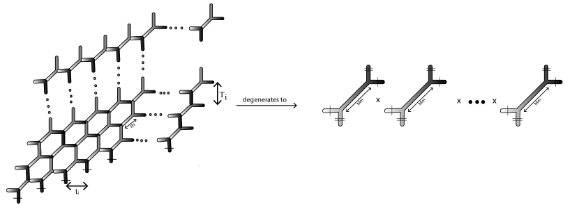
Figure 6: $\mathcal{Z}_{N,M}$ degenerating to $(\mathcal{Z}_{1,1})^{N}$

5.4 Interpreting the factorisation: $\mathcal{Z}_{(M,N)}$ $\to$ $\mathcal{Z}_{(1,1)}^{N}$

Recall that, on a arbitrary point of the Kähler cone, the number of independent Kähler parameters entering the partition function are

$$\#(T_{a}s)+\#(t_{i}s)+\#(\mbox{intersections})-\#(\mbox{horizontal}\quad\mbox{constraints})-\#(\mbox{vertical}\quad\mbox{constraints})+2$$

$$=(M-1)+(N-1)+MN-(M-1)-(N-1)+2$$

$$=MN+2$$ (5.9)

In general we can have three different series representations Hohenegger_2017 of $Z_{(M,N)}$ according to whether the toric web diagram of $X_{M,N}$ is sliced into horizontal strips, vertical strips and diagonal strips

$$\displaystyle\mathcal{Z}_{(M,N)}(\textbf{t},\textbf{T},\textbf{m},\epsilon_{1},\epsilon_{2}) = \mathcal{Z}^{pert}(\textbf{T},\textbf{m})\sum_{\vec{k}}e^{-\vec{k}.\textbf{t}}\mathcal{Z}_{\vec{k}}(\textbf{T},\textbf{m})$$

$$\mathcal{Z}_{(M,N)}(\textbf{t},\textbf{T},\textbf{m},\epsilon_{1},\epsilon_{2}) = \mathcal{Z}^{pert}(\textbf{t},\textbf{m})\sum_{\vec{k}}e^{-\vec{k}.\textbf{T}}\mathcal{Z}_{\vec{k}}(\textbf{t},\textbf{m})$$

$$\mathcal{Z}_{(M,N)}(\textbf{t},\textbf{T},\textbf{m},\epsilon_{1},\epsilon_{2}) = \mathcal{Z}^{pert}(\textbf{T},\textbf{t})\sum_{\vec{k}}e^{-\vec{k}.\textbf{m}}\mathcal{Z}_{\vec{k}}(\textbf{T},\textbf{t})$$ (5.10)

where the Kähler parameters $T_{i}$ from $\bf{T}$$=\{T_{1},T_{2},...,T_{M}\}$ represent the distance between vertical lines , $t_{i}$ from $\bf{t}$$=\{t_{1},t_{2},...,t_{N}\}$ represent the distance between horizontal lines and $\bf{m}$ denote the diagonal lines of the web diagram in figure 5. These expansion have been interpreted as instanton expansions of three gauge theories which are dual to each other. For these to be consistent expansions it is assumed that there exists a region of the moduli space of $X_{(M,N)}$ in which either T or t or m become infinite, with all the rest of parameters kept finite. This region of the moduli space corresponds to the weak coupling limit of gauge theories.
At the special point in the moduli space where $t_{a,a+1}=m$, we are left with three independent Kähler parameters $\tau,\rho,m$. Moreover due to the weak coupling expansion $\{\textbf{T}\to\infty\}$, $N$ horizontal strips gets decoupled and we get $Z_{1,1}^{N}$.

Remark:

After normalisation by the gauge theory perturbative part, the partition function $Z_{(1,1)}(\tau,\rho,\,m)$ can be written as Dijkgraaf:2007sw ; Bousseau:2020ckw ; lockhart2012superconformal

$$\displaystyle\mathcal{Z}_{(1,1)}(\,\tau,\rho,m) = e^{\frac{-\pi i(\tau+\rho+m)}{12}}\prod_{(k,l,m)>0}(1-e^{2\pi i(k\tau+l\rho+pm)})^{-c(4kl-p^{2})}$$ (5.11)

$$= \frac{1}{\Phi_{10}(\tau,\rho,m)^{\frac{1}{24}}}$$

where $c(4kl-p^{2})$ are the Fourier coefficients of the elliptic genus of $K3$

$$\displaystyle\chi(K3,\tau,z)=\sum_{h\geq 0,m\in\mathbb{Z}}24c(4h-m^{2})e^{2\pi i(h\tau+mz)}$$ (5.12)

and $\Phi_{10}(\tau,\rho,m)$ is the unique weight $10$ automorphic form of $Sp(2,\mathbb{Z})$. We have implicit used the fact that the large radius limit (universal part) of the Taub-NUT elliptic genus matches with the elliptic genus of $\mathbb{C}^{2}$ Harvey:2014nha . This allows us to write $Z_{(N,M)}(\tau,\rho,t_{a,a+1}=m)$ in the following way

$$\displaystyle\mathcal{Z}_{(N,M)}(\tau,\rho,t_{a,a+1}=m) = e^{\frac{-N\pi i(\tau+\rho+m)}{12}}\prod_{(k,l,m)>0}(1-e^{2\pi i(Mk\tau+l\rho+pMm)})^{-Nc(4kl-p^{2})}$$ (5.13)

$$= \frac{1}{\Phi_{10}(M\tau,\rho,Mm)^{\frac{N}{24}}}$$

6 Degeneration 2:Splitting Degeneration

This degeneration corresponds to turning off the Kähler parameters in such a way that the partition function $\mathcal{Z}_{N,M}$ reduces to the partition function $\mathcal{Z}_{N,M-1}$, upto an overall factor of Dedekind eta function. Consider the following partition function

$$\displaystyle\mathcal{Z}_{(N,M)}(\tau,\rho,m_{a}\,,\epsilon_{1,2},\widetilde{t}_{ab}) =\sum_{\alpha_{a}^{i}}\,\prod_{i=1}^{N}Q_{i}^{|\alpha^{(i)}|}\,\prod_{i=1}^{N}\prod_{a=1}^{M}\,\frac{\vartheta_{\alpha_{a}^{i+1}\alpha_{a}^{i}}(m_{a})}{\vartheta_{\alpha_{a}^{i}\alpha_{a}^{i}}(\epsilon_{+})}$$ (6.1)

$$\prod_{1\leq a<b\leq M}\prod_{i=1}^{N}\frac{\vartheta_{\alpha_{a}^{i}\alpha_{b}^{i+1}}(\widetilde{t}_{ab})\vartheta_{\alpha_{a}^{i+1}\alpha_{b}^{i}}(\widetilde{t}_{ab}+m_{a}+m_{b})}{\vartheta_{\alpha_{a}^{i}\alpha_{b}^{i}}(\widetilde{t}_{ab}+m_{a}-\epsilon_{+})\vartheta_{\alpha_{a}^{i}\alpha_{b}^{i}}(\widetilde{t}_{ab}+m_{b}+\epsilon_{+})}.$$

In the above partition function (6.1)

$$\widetilde{t}_{ab}=\widetilde{t}_{a\,a+1}+m_{a+1}+\widetilde{t}_{a+1\,a+2}+\cdots+m_{b-1}+\widetilde{t}_{b-1\,b}.$$

For $N=1$ the above defined partition function reduces to

$$\displaystyle\mathcal{Z}_{(1,M)}(\tau,\rho,m_{a}\,,\epsilon_{1,2}\,,\widetilde{t_{ab}}) =\sum_{\alpha_{1,2,\cdots,M}}\,Q^{|\alpha_{1}|+\cdots+|\alpha_{M}|}\,\prod_{a=1}^{M}\frac{\vartheta_{\alpha_{a}\alpha_{a}}(m_{a})}{\vartheta_{\alpha_{a}\alpha_{a}}(\epsilon_{+})}$$

$$\prod_{1\leq a<b\leq M}\frac{\vartheta_{\alpha_{a}\alpha_{b}}(\widetilde{t_{ab}})\vartheta_{\alpha_{a}\alpha_{b}}(\widetilde{t_{ab}}+m_{a}+m_{b})}{\vartheta_{\alpha_{a}\alpha_{b}}(\widetilde{t_{ab}}+m_{a}-\epsilon_{+})\vartheta_{\alpha_{a}\alpha_{b}}(\widetilde{t_{ab}}+m_{b}+\epsilon_{+})}$$

Remark:

Note that $\sum_{\mu}Q^{|\mu|}=\frac{e^{\frac{\pi i}{12}}}{\eta(\tau)}$. This factor appears in the degeneration limit as discussed below.

6.1 $(N,M)=(1,2)$

Let us consider the partition function for $N=1$ and $M=2$ in the unrefined case ($\epsilon_{1}=-\epsilon_{2}=\epsilon$),

$$\displaystyle\mathcal{Z}_{(1,2)}(\tau,\rho,m_{1,2},\widetilde{t_{12}},\epsilon)=\sum_{\alpha_{1,2}}\,Q^{|\alpha_{1}|+|\alpha_{2}|}\,\frac{\vartheta_{\alpha_{1}\alpha_{1}}(m_{1})\vartheta_{\alpha_{2}\alpha_{2}}(m_{2})}{\vartheta_{\alpha_{1}\alpha_{1}}(0)\vartheta_{\alpha_{2}\alpha_{2}}(0)}\frac{\vartheta_{\alpha_{1}\alpha_{2}}(\widetilde{t_{12}})\vartheta_{\alpha_{1}\alpha_{2}}(\widetilde{t_{12}}+m_{1}+m_{2})}{\vartheta_{\alpha_{1}\alpha_{2}}(\widetilde{t_{12}}+m_{1})\vartheta_{\alpha_{1}\alpha_{2}}(\widetilde{t_{12}}+m_{2})}$$ (6.2)

$\bullet\quad\mathbf{m_{1}\rightarrow 0}$ or $\mathbf{m_{2}\rightarrow 0}$:
When we take $m_{1}=0$ in the partition function (6.2), the terms in the numerator and denominator becomes same, therefore they cancel out each other. Then (6.2) reduces to the multiple of $Z_{(1,1)}$ as:

$$\displaystyle\mathcal{Z}_{(1,2)}(\tau,\rho,m_{2},\widetilde{t_{12}},\epsilon) =\sum\limits_{\alpha_{1,2}}\,Q^{|\alpha_{1}|+|\alpha_{2}|}\,\frac{\vartheta_{\alpha_{2}\alpha_{2}}(m_{2})}{\vartheta_{\alpha_{2}\alpha_{2}}(0)}$$

$$=\sum\limits_{\alpha_{1}}Q^{|\alpha_{1}|}\mathcal{Z}_{(1,1)}(\tau,\rho,m_{2},\epsilon)$$

Same result follows for the case when we take $m_{2}=0$ in (6.2) i.e,

$$\displaystyle\mathcal{Z}_{(1,2)}(\tau,\rho,m_{1},\widetilde{t_{12}},\epsilon)=\sum_{\alpha_{2}}Q^{|\alpha_{2}|}\mathcal{Z}_{(1,1)}(\tau,\rho,m_{2},\epsilon)$$

$\bullet$  $\widetilde{\mathbf{t}_{12}}\rightarrow 0:$
In the limit $\widetilde{t_{12}}\rightarrow 0$, (6.2) is:

$$\displaystyle\mathcal{Z}_{(1,2)}(\tau,\rho,m_{1,2},\epsilon)=\sum_{\alpha_{1,2}}\,Q^{|\alpha_{1}|+|\alpha_{2}|}\,\frac{\vartheta_{\alpha_{1}\alpha_{1}}(m_{1})\vartheta_{\alpha_{2}\alpha_{2}}(m_{2})}{\vartheta_{\alpha_{1}\alpha_{1}}(0)\vartheta_{\alpha_{2}\alpha_{2}}(0)}\frac{\vartheta_{\alpha_{1}\alpha_{2}}(0)\vartheta_{\alpha_{1}\alpha_{2}}(m_{1}+m_{2})}{\vartheta_{\alpha_{1}\alpha_{2}}(m_{1})\vartheta_{\alpha_{1}\alpha_{2}}(m_{2})}$$ (6.3)

Again, the presence of $\vartheta_{\alpha_{1}\alpha_{1}}(0)$ force contribution only from the same partition and we get the following:

$$\mathcal{Z}_{(1,2)}(\tau,\rho,m_{1,2},\epsilon)=\mathcal{Z}_{(1,1)}(2\tau,\rho,m_{1}+m_{2},\epsilon)$$

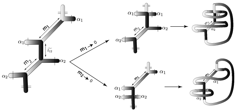
Figure 7: Two possible degenerations of the partition function $Z_{1,2}$. The third column depicts 3D/non-planar structure of the mirror curves

6.2 $(N,M)=(1,3)$

Similarly consider the partition function $\mathcal{Z}_{(1,3)}(\tau,\rho,m_{1,2,3},\widetilde{t}_{a,b},\epsilon)$

$$\mathcal{Z}_{(1,3)}(\tau,\rho,m_{1,2,3},\widetilde{t}_{a,b},\epsilon)=\sum\limits_{\alpha_{1,2,3}}\,Q^{\sum\limits_{k=1}^{3}|\alpha_{k}|}\,\left(\prod_{k=1}^{3}\frac{\vartheta_{\alpha_{k}\alpha_{k}}(m_{k})}{\vartheta_{\alpha_{k}\alpha_{k}}(0)}\right)\frac{\vartheta_{\alpha_{1}\alpha_{2}}(\widetilde{t_{12}})\vartheta_{\alpha_{1}\alpha_{2}}(\widetilde{t_{12}}+m_{1}+m_{2})}{\vartheta_{\alpha_{1}\alpha_{2}}(m_{1}+\widetilde{t_{12}})\vartheta_{\alpha_{1}\alpha_{2}}(m_{2}+\widetilde{t_{12}})}$$

$$\quad\quad\quad\quad\frac{\vartheta_{\alpha_{2}\alpha_{3}}(\widetilde{t_{23}})\vartheta_{\alpha_{2}\alpha_{3}}(\widetilde{t_{23}}+m_{2}+m_{3})}{\vartheta_{\alpha_{2}\alpha_{3}}(\widetilde{t_{23}}+m_{2})\vartheta_{\alpha_{2}\alpha_{3}}(\widetilde{t_{23}}+m_{3})}\frac{\vartheta_{\alpha_{1}\alpha_{3}}(\widetilde{t_{13}})\vartheta_{\alpha_{1}\alpha_{3}}(\widetilde{t_{13}}+m_{1}+m_{3})}{\vartheta_{\alpha_{1}\alpha_{3}}(\widetilde{t_{13}}+m_{1})\vartheta_{\alpha_{1}\alpha_{3}}(\widetilde{t_{13}}+m_{3})}$$ (6.4)

Figure 8: $Z_{13}$

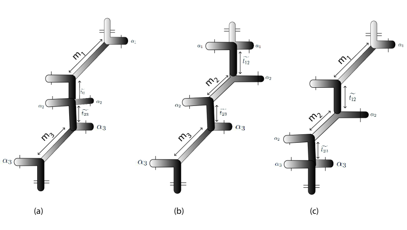
Figure 9: Three possible degenerations of the partition function $Z_{1,3}$.

Remember here all $m_{i}^{\prime}$s $i=1,2,3$ are different, and $\widetilde{t_{13}}=\widetilde{t_{12}}+m_{2}+\widetilde{t_{23}}.$

$\bullet$ $\mathbf{m_{3}\mapsto 0}:$
When $m_{3}$ approaches to zero in (LABEL:Z13) it takes the following form:

$$\displaystyle\mathcal{Z}_{(1,3)}(\tau,\rho,m_{1,2},\widetilde{t_{12}},\epsilon) =\sum_{\alpha_{1,2,3}}\,Q^{|\alpha_{1}|+|\alpha_{2}|+|\alpha_{3}|}\,\frac{\vartheta_{\alpha_{1}\alpha_{1}}(m_{1})\vartheta_{\alpha_{2}\alpha_{2}}(m_{2})}{\vartheta_{\alpha_{1}\alpha_{1}}(0)\vartheta_{\alpha_{2}\alpha_{2}}(0)}\frac{\vartheta_{\alpha_{1}\alpha_{2}}(\widetilde{t_{12}})\vartheta_{\alpha_{1}\alpha_{2}}(\widetilde{t_{12}}+m_{1}+m_{2})}{\vartheta_{\alpha_{1}\alpha_{2}}(m_{1}+\widetilde{t_{12}})\vartheta_{\alpha_{1}\alpha_{2}}(m_{2}+\widetilde{t_{12}})}$$

$$=\sum_{\alpha_{3}}Q^{|\alpha_{3}|}\,\mathcal{Z}_{(1,2)}(\tau,\rho,m_{1,2},\widetilde{t_{12}},\epsilon)$$

Thus $Z_{(1,3)}\rightarrow Z_{(1,2)}$.

$\bullet$ $\mathbf{m_{2}\mapsto 0}:$
Similarly

$$\displaystyle\mathcal{Z}_{(1,3)}(\tau,\rho,m_{1,2,3},\widetilde{t_{13}},\epsilon)\quad\underrightarrow{m_{2}=0}\quad\sum_{\alpha_{2}}Q^{|\alpha_{2}|}\,\mathcal{Z}_{(1,2)}(\tau,\rho,m_{1,3},\widetilde{t_{13}},\epsilon)$$

and
$\bullet$ $\mathbf{m_{1}\mapsto 0}:$

$$\displaystyle\mathcal{Z}_{(1,3)}(\tau,\rho,m_{1,2,3},\widetilde{t_{23}},\epsilon)\quad\underrightarrow{m_{1}=0}\quad\sum_{\alpha_{1}}Q^{|\alpha_{1}|}\,\mathcal{Z}_{(1,2)}(\tau,\rho,m_{2,3},\widetilde{t_{23}},\epsilon)$$

Hence in all these three cases when any $m_{1},m_{2}$ or $m_{3}$ is zero $\mathcal{Z}_{(1,3)}$ reduces to the case of $\mathcal{Z}_{(1,2)}$ upto some factor. Moreover same degeneration of $\mathcal{Z}_{1,3}$ results if one takes the limit $\widetilde{t_{ab}}\rightarrow 0$ for any $a,b$ i.e., $\mathcal{Z}_{(1,3)}\to\mathcal{Z}_{(1,2)}$.
$\bullet$ $\mathbf{\widetilde{t}_{ab}\mapsto 0}:$

$$\displaystyle\mathcal{Z}_{(1,3)}(\tau,\rho,m_{1,2,3},\widetilde{t_{23}},\epsilon)\quad\underrightarrow{\widetilde{t}_{ab}=0}\quad\sum_{\alpha}Q^{|\alpha|}\,\mathcal{Z}_{(1,2)}(\tau,\rho,m_{1,2,3},\epsilon)$$

6.3 $(N,M)=(2,3)$

Previous subsections discuss the cases when $N=1$ and now we generalize to the case of $N=2$. Explicitly the partition function is of the form

$$\displaystyle\mathcal{Z}_{(2,3)}(\tau,\rho,m_{1,2,3},\epsilon_{1,2},\widetilde{t}_{ab}) = \sum_{\alpha_{a}^{i}}\,\prod_{i=1}^{2}Q_{i}^{|\alpha^{(i)}|}\,\prod_{i=1}^{2}\prod_{a=1}^{3}\,\frac{\vartheta_{\alpha_{a}^{i+1}\alpha_{a}^{i}}(m_{a})}{\vartheta_{\alpha_{a}^{i}\alpha_{a}^{i}}(0)}$$ (6.5)

$$\times \prod_{1\leq a<b\leq 3}\prod_{i=1}^{2}\frac{\vartheta_{\alpha_{a}^{i}\alpha_{b}^{i+1}}(\widetilde{t_{ab}})\vartheta_{\alpha_{a}^{i+1}\alpha_{b}^{i}}(\widetilde{t_{ab}}+m_{a}+m_{b})}{\vartheta_{\alpha_{a}^{i}\alpha_{b}^{i}}(\widetilde{t_{ab}}+m_{a}-\epsilon_{+})\vartheta_{\alpha_{a}^{i}\alpha_{b}^{i}}(\widetilde{t_{ab}}+m_{b}+\epsilon_{+})}$$

For the unrefined case $\epsilon_{1}=-\epsilon_{2}=\epsilon$, we consider the degenerate limit $m_{3}=0$. Using the identity (4.5) we get

$$\mathcal{Z}_{(2,3)}(\tau,\rho,m_{1,2},m_{3}=0,\widetilde{t}_{ab},\epsilon)=\sum_{\alpha^{1},\alpha^{2},\alpha_{3}^{(1)}}\,Q_{1}^{|\alpha^{(1)}|}Q_{2}^{|\alpha^{(2)}|}(Q_{1}Q_{2})^{|\alpha_{3}^{(1)}|}\,\frac{\vartheta_{\alpha_{1}^{(2)}\alpha_{1}^{(1)}}(m_{1})\vartheta_{\alpha_{2}^{(2)}\alpha_{2}^{(1)}}(m_{2})}{\vartheta_{\alpha_{1}^{(1)}\alpha_{1}^{(1)}}(0)\vartheta_{\alpha_{2}^{(1)}\alpha_{2}^{(1)}}(0)}$$

$$\frac{\vartheta_{\alpha_{1}^{(1)}\alpha_{1}^{(2)}}(m_{1})\vartheta_{\alpha_{2}^{(1)}\alpha_{2}^{(2)}}(m_{2})}{\vartheta_{\alpha_{1}^{(2)}\alpha_{1}^{(2)}}(0)\vartheta_{\alpha_{2}^{(2)}\alpha_{2}^{(2)}}(0)}\frac{\vartheta_{\alpha_{1}^{(1)}\alpha_{2}^{(2)}}(\widetilde{t_{12}})\vartheta_{\alpha_{1}^{(2)}\alpha_{2}^{(1)}}(\widetilde{t_{12}}+m_{1}+m_{2})}{\vartheta_{\alpha_{1}^{(1)}\alpha_{2}^{(1)}}(\widetilde{t_{12}}+m_{1})\vartheta_{\alpha_{1}^{(1)}\alpha_{2}^{(1)}}(\widetilde{t_{12}}+m_{2})}\frac{\vartheta_{\alpha_{1}^{(2)}\alpha_{2}^{(1)}}(\widetilde{t_{12}})\vartheta_{\alpha_{1}^{(1)}\alpha_{2}^{(2)}}(\widetilde{t_{12}}+m_{1}+m_{2})}{\vartheta_{\alpha_{1}^{(2)}\alpha_{2}^{(2)}}(\widetilde{t_{12}}+m_{1})\vartheta_{\alpha_{1}^{(2)}\alpha_{2}^{(2)}}(\widetilde{t_{12}}+m_{2})}$$

Recognizing the $\mathcal{Z}_{(2,2)}(\tau,\rho,m_{1,2},t_{ab},\epsilon)$ part, the last expression can be written more succinctly as

$$\displaystyle\mathcal{Z}_{(2,3)}(\tau,\rho,m_{1,2},m_{3}=0,\widetilde{t}_{ab},\epsilon) = \sum_{\alpha_{3}^{(1)}}Q_{1}^{\alpha_{3}^{(1)}}Q_{2}^{\alpha_{3}^{(1)}}\mathcal{Z}_{(2,2)}(\tau,\rho,m_{1,2},\widetilde{t}_{ab},\epsilon)$$ (6.6)

Similar degenerations follow by taking the limit $m_{2}=0$ or $m_{1}=0$.

6.4 General $(N,M)$

The previous sections discuss the cases when $N$ was taken equal to one. In this section we generalize the argument to generic values of $M$ and $N.$ For the unrefined case $\epsilon_{1}=-\epsilon_{2}=\epsilon$

$$\displaystyle\mathcal{Z}_{(N,M)}(\tau,\rho,m_{a},\epsilon_{1,2},\widetilde{t}_{ab}) = \sum_{\alpha_{a}^{i}}\,\prod_{i=1}^{N}Q_{i}^{|\alpha^{(i)}|}\,\prod_{i=1}^{N}\prod_{a=1}^{M}\,\frac{\vartheta_{\alpha_{a}^{i+1}\alpha_{a}^{i}}(m_{a})}{\vartheta_{\alpha_{a}^{i}\alpha_{a}^{i}}(0)}$$ (6.7)

$$\times \prod_{1\leq a<b\leq M}\prod_{i=1}^{N}\frac{\vartheta_{\alpha_{a}^{i}\alpha_{b}^{i+1}}(\widetilde{t_{ab}})\vartheta_{\alpha_{a}^{i+1}\alpha_{b}^{i}}(\widetilde{t_{ab}}+m_{a}+m_{b})}{\vartheta_{\alpha_{a}^{i}\alpha_{b}^{i}}(\widetilde{t_{ab}}+m_{a})\vartheta_{\alpha_{a}^{i}\alpha_{b}^{i}}(\widetilde{t_{ab}}+m_{b})}$$

$$\displaystyle\mathcal{Z}_{(N,M)}(\tau,\rho,m_{a},\widetilde{t}_{ab},\epsilon) = \sum_{\alpha_{a}^{i}}\,\prod_{i=1}^{N}Q_{i}^{|\alpha^{(i)}|}\,\prod_{i=1}^{N}\prod_{a=1}^{M}\,\frac{\vartheta_{\alpha_{a}^{i+1}\alpha_{a}^{i}}(m_{a})}{\vartheta_{\alpha_{a}^{i}\alpha_{a}^{i}}(0)}$$

$$\times \prod_{a=1}^{M-1}\prod_{b=a+1}^{M}\frac{\vartheta_{\alpha_{a}^{i}\alpha_{b}^{i+1}}(\widetilde{t}_{a\,a+1}+m_{a+1}+\widetilde{t}_{a+1\,a+2}+\cdots+m_{b-1}+\widetilde{t}_{b-1\,b})}{\vartheta_{\alpha_{a}^{i}\alpha_{b}^{i}}(\widetilde{t}_{a\,a+1}+m_{a+1}+\widetilde{t}_{a+1\,a+2}+\cdots+m_{b-1}+\widetilde{t}_{b-1\,b})}$$

$$\times \frac{\vartheta_{\alpha_{a}^{i}\alpha_{b}^{i+1}}(\widetilde{t}_{a\,a+1}+m_{a+1}+\widetilde{t}_{a+1\,a+2}+\cdots+m_{b-1}+\widetilde{t}_{b-1\,b}+m_{a}+m_{b})}{\vartheta_{\alpha_{a}^{i}\alpha_{b}^{i}}(\widetilde{t}_{a\,a+1}+m_{a+1}+\widetilde{t}_{a+1\,a+2}+\cdots+m_{b-1}+\widetilde{t}_{b-1\,b})}$$

Specializing to $N=1$, $Q_{i}=Q$ and in the limit $m_{1}=0$ the last expression reduces to

$$\displaystyle\mathcal{Z}_{(1,M)}(\tau,\rho,m_{a},\widetilde{t}_{ab},\epsilon) = \sum_{\alpha_{1}}Q^{|\alpha_{1}|}\mathcal{Z}_{(1,M-1)}(\tau,\rho,m_{i}\,,\widetilde{t}_{ab},\epsilon)$$ (6.9)

where $t_{ab}$ and $m_{i}$ do not include the moduli which are tuned to zero. More generally and at the same point $Q_{i}=Q$ in the moduli space we expect similar structure for $\mathcal{Z}_{(N,M)}$

$$\displaystyle\mathcal{Z}_{(N,M)}(\tau,\rho,m_{a},\widetilde{t}_{ab},\epsilon) = \sum_{\alpha_{a}^{i}}\,\prod_{i=1}^{N}Q^{|\alpha^{(i)}|}\,\prod_{i=1}^{N}\prod_{a=2}^{M}\,\frac{\vartheta_{\alpha_{a}^{i+1}\alpha_{a}^{i}}(m_{a})}{\vartheta_{\alpha_{a}^{i}\alpha_{a}^{i}}(0)}$$

$$\times \prod_{a=2}^{M-1}\prod_{b=a+1}^{M}\frac{\vartheta_{\alpha_{a}^{i}\alpha_{b}^{i+1}}(\widetilde{t}_{aa+1}+\widetilde{t}_{a+1a+2}+...+\widetilde{t}_{b-1b}+m_{a+1}+...+m_{b-1})}{\vartheta_{\alpha_{a}^{i}\alpha_{b}^{i}}(\widetilde{t}_{aa+1}+\widetilde{t}_{a+1a+2}+...+\widetilde{t}_{b-1b}+m_{a}+m_{a+1}+...+m_{b-1})}$$

$$\times \frac{\vartheta_{\alpha_{a}^{i}\alpha_{b}^{i+1}}(\widetilde{t}_{aa+1}+\widetilde{t}_{a+1a+2}+...+\widetilde{t}_{b-1b}+m_{a}+m_{a+1}+...+m_{b-1}+m_{b})}{\vartheta_{\alpha_{a}^{i}\alpha_{b}^{i}}(\widetilde{t}_{aa+1}+\widetilde{t}_{a+1a+2}+...+\widetilde{t}_{b-1b}+m_{a+1}+...+m_{b-1}+m_{b})}$$

$$\times \prod_{i=1}^{N}\frac{\vartheta_{\alpha_{1}^{i+1}\alpha_{1}^{i}}(m_{1})}{\vartheta_{\alpha_{1}^{i}\alpha_{1}^{i}}(0)}\bigg{(}\frac{\vartheta_{\alpha_{1}^{i}\alpha_{2}^{i+1}}(\widetilde{t}_{12})\vartheta_{\alpha_{1}^{i}\alpha_{2}^{i+1}}(\widetilde{t}_{12}+m_{1}+m_{2})}{\vartheta_{\alpha_{1}^{i}\alpha_{2}^{i}}(\widetilde{t}_{12}+m_{1})\vartheta_{\alpha_{1}^{i}\alpha_{2}^{i}}(\widetilde{t}_{12}+m_{2})}$$

$$\times \frac{\vartheta_{\alpha_{1}^{i}\alpha_{3}^{i+1}}(\widetilde{t}_{12}+\widetilde{t}_{23}+m_{2})\vartheta_{\alpha_{1}^{i}\alpha_{3}^{i+1}}(\widetilde{t}_{12}+\widetilde{t}_{23}+m_{1}+m_{2}+m_{3})}{\vartheta_{\alpha_{1}^{i}\alpha_{3}^{i}}(\widetilde{t}_{12}+\widetilde{t}_{23}+m_{1}+m_{2})\vartheta_{\alpha_{1}^{i}\alpha_{3}^{i}}(\widetilde{t}_{12}+\widetilde{t}_{23}+m_{2}+m_{3})}$$

$$... \times \frac{\vartheta_{\alpha_{1}^{i}\alpha_{M}^{i+1}}(\widetilde{t}_{12}+\widetilde{t}_{23}+...+\widetilde{t}_{M-1M}+m_{1}+m_{2}+...+m_{M-1}+m_{M})}{\vartheta_{\alpha_{1}^{i}\alpha_{M}^{i+1}}(\widetilde{t}_{12}+\widetilde{t}_{23}+...+\widetilde{t}_{M-1M}+m_{2}+...+m_{M-1}+m_{M})}\bigg{)}$$

In the limit $m_{1}\to 0$

$$\displaystyle\mathcal{Z}_{(N,M)}(\tau,\rho,m_{a},\widetilde{t}_{ab},\epsilon) = \big{(}\sum_{\alpha_{1}^{i}}\prod_{i=1}^{N}Q^{\alpha_{1}^{(i)}}\big{)}\mathcal{Z}_{(N,M-1)}(\tau,\rho,m_{q},\widetilde{t}_{pq},\epsilon)$$

Similar recursive structure in (N,M) shows up in the limits $m_{i}=0$ (for any i=2,…) or $\tilde{t}_{i}=0$. From mathematical viewpoint such degenerations have been discussed in li1998symplectic ; liu2005transformation .

7 Discussions

The compactified 5-brane web given in fig.5 gives rise to a five dimensional $\mathcal{N}=2$ supersymmetric gauge theory on the common worldvolume. This 5-branes web can be deformed to include also $(1,1)$ 5-branes. In string theory this is interpreted as the splitting of the D5-branes on the NS5-brane world volume. In other words the string tension is turned on for the strings that are stretched between D5-branes. It gives rise to the mass deformation of the bifundamental hypermultiplets in the five dimensional gauge theory. The mass deformation results in the breaking of supersymmetry to $\mathcal{N}=1$ in five dimensions. Because of the toric compactification of the 5-branes web one gets affine $\hat{A}_{N-1}$ quiver gauge theory with an $SU(N)$ gauge group at each node and one bifundamental matter stretched between adjacent nodes. There are $M$ coupling constants $\tau_{i},i=1,...,M$ for each node such that

$$\displaystyle\sum_{i=1}^{M}\tau_{i}=\frac{1}{R_{1}}$$ (7.1)

where $R_{1}$ is the radius of the $S^{1}$ on which M5-brane theory is compactified. In geometrical terms each gauge coupling constant is related to the area of a distinct curve in CY threefold. If there are more than one, though equivalent, choices of these curves, this gives rise to dual gauge theory formulations of the same system. In other words for the web of $M$ NS5-branes and $N$ D5-branes the gauge theory on the D5-branes is given by

gauge group $$:U(1)\times SU(N)_{1}\times SU(N)_{2}\times...\times SU(N)_{M}$$

hypermultiplet representation $$:\oplus_{i=1}^{M}\bigg{(}(N_{a},\bar{N}_{a+1})\oplus(\bar{N}_{a},N_{a+1})\bigg{)}$$ (7.2)

where $N_{a}$ is the $SU(N)$ fundamental representation of the a-th node and $\bar{N}_{a}$ the complex conjugate one. The partition function of the quiver gauge theories given in (7) can be computed directly by using Nekrasov instanton calculus as described in Hohenegger:2013ala . In doing so one has to take into account the non-trivial winding of strings on the compact direction transverse to the 5-branes. There is interesting physical interpretations of these degenerations. In the previous sections we have discussed how various degenerations of the mirror curve is related to certain degeneration of the corresponding partition functions $\mathcal{Z}_{(N,M)}$. Recall the following degeneration (5.8)

$$\displaystyle\mathcal{Z}_{(N,M)}(\tau,\rho,t_{a,a+1}=m,\epsilon)=\mathcal{Z}_{(1,1)}(M\,\tau,\rho,M\,m,\epsilon)^{N}$$ (7.3)

This degeneration corresponds to a $U(N)^{M}$ quiver gauge theory degenerating to a $U(1)^{M}$ gauge theory. Moreover the gauge coupling constant $\tau$ and the hypermultiplet mass parameter $m$ are scaled to $M\tau$ and $Mm$ under the degeneration. This rescaling corresponds to multiple wrapping number of the D-branes along the $\tau$ and $m$ directions.
Similarly the second degeneration of the $\mathcal{Z}_{N,M}$ (6.4) that we discussed and is given by

$$\displaystyle\mathcal{Z}_{(N,M)}(\tau,\rho,m_{a},t_{ab},\epsilon) = \big{(}\sum_{\alpha_{1}^{i}}\prod_{i=1}^{N}Q_{i}^{\alpha_{1}^{(i)}}\big{)}\mathcal{Z}_{(N,M-1)}(\tau,\rho,m_{q},\widetilde{t}_{pq},\epsilon)$$

has an interesting physical interpretation. The limit $m_{i}\to 0$ corresponds to supersymmetry enhancement to $N=4$ and we get a decoupling factor of $\eta(\tau)$.

8 Conclusions

This paper explored some interesting consequences of the mirror symmetry of the local CY threefold $X_{N,M}$. We investigated some interesting properties of the type $A$ topological string partition function of $X_{N,M}$ in special regions of the Kähler moduli space. We have called these degenerate limits, because in these limits the partition functions on $X_{N,M}$ collapse to those on $X_{N,M-1}$ in various ways. In accordance with mirror symmetry the degeneration behaviour on the type A side is reproduced on the type B side in the degeneration of the mirror curves into lower genus curves.
For future directions it would be interesting to study the analogous properties of $\mathcal{Z}_{N,M}$ and quantum mirror curves for the general $\Omega$-background .i.e. $\epsilon_{1}\neq 0$ and/or $\epsilon_{1}\neq 0$ and $\epsilon_{1}\neq\epsilon_{2}$ and at an arbitrary point of the Kähler moduli space of $X_{N,M}$. It will also be interesting to study the modular properties of the free energy $\log(\hat{\mathcal{Z}}_{(N,M)}(\tau,\rho,\epsilon,m,\mbox{\bf{t}}))$ and the single particle free energy Hohenegger:2015cba $PLog(\hat{\mathcal{Z}}_{(N,M)}(\tau,\rho,\epsilon,m,\mbox{\bf{t}}))$ along the lines of Hohenegger_2020 . It is also interesting to generalise the quantisation of classical DELL system as done in Koroteev:2019gqi to the case where the underlying abelian variety has (M,N) polarization.

Appendix A         
Geometry of $X_{N,M}$: a quick review

The non-compact CY 3-fold $X_{1,1}$ is defined as the partial compactification Kanazawa:2016tnt ; Hohenegger:2013ala of the resolved conifold geometry. The later is given by $\mathbb{C}^{\times}\times\mathbb{C}^{\times}$ fibered over the $z$-plane. The partial compactification is achieved by compactifying each of the two $\mathbb{C}^{\times}$ fibers to a $\mathbb{T}^{2}$ fiber. Of the three Kähler parameters $\tau,\rho,m$ of the CY 3-fold $X_{1,1}$, $\rho$ and $\tau$ correspond to the elliptic fibers and $m$ corresponds to the curve class of the exceptional $\mathbb{P}^{1}$ of the resolved conifold. We will define the non-compact CY 3-fold $X_{N,M}$ for $N,M\in\mathbb{N}$ as the $\mathbb{Z}_{N}\times\mathbb{Z}_{M}$ orbifold of $X_{1,1}$.
In toric geometry the equation of the conifold given by

$$\displaystyle z_{1}z_{2}-z_{3}z_{4}=0,\quad z_{1},z_{2},z_{2},z_{4}\in\mathbb{C}$$ (A.1)

is translated to an equation on integer latices parametrised by 3-vectors $v_{1},v_{2},v_{3},v_{4}$

$$\displaystyle v_{1}+v_{2}-v_{3}-v_{4}=0.$$ (A.2)

The CY condition constrains the geometry to a plane. The irreducible toric rational curves of the 2-dimensional cone are given by

$$\displaystyle C^{1}_{(a,b)}: = \mathbb{R}_{\geq 0}Conv(\{(a+1,b,1),(a,b+1,1)\}),\quad C^{2}_{(a,b)}:=\mathbb{R}_{\geq 0}Conv(\{(a,b,1),(a,b+1,1)\}),$$

$$C^{3}_{(a,b)}: = \mathbb{R}_{\geq 0}Conv(\{(a,b,1),(a+1,b,1)\}).$$ (A.3)

for all $a,b\in\mathbb{Z}$. The Kähler variables $q_{i}$ corresponding to $C^{i}$ are defined as the exponential of the symplectic area of $C^{i}$. The author in Kanazawa:2016tnt computes Strominger-Yau-Zaslow (SYZ) Strominger:1996it mirror of the local CY3-fold $X_{N,M}$, which is given by

$$\displaystyle uv=\sum_{a,b=0}^{N-1,M-1}\Delta_{a,b}\sum_{c,d\in\mathbb{Z}^{2}}q^{C_{(cN+a,dM+b)}}z_{1}^{cN+a}z_{2}^{dM+b}$$ (A.4)

where $\Delta_{a,b}$ encodes the data of the open Gromov-Witten invariants, $z_{1},z_{2}$ are coordinates of the abelian variety of polarisation $(N,M)$, and $u,v$ are the sections of certain line bundles on the abelian variety. The zero locus

$$\displaystyle\sum_{a,b=0}^{N-1,M-1}\Delta_{a,b}\sum_{c,d\in\mathbb{Z}^{2}}q^{C_{(cN+a,dM+b)}}z_{1}^{cN+a}z_{2}^{dM+b}=0$$ (A.5)

defines a curve with genus $NM+1$ with $(N,M)$ polarisation. For illustration, consider the CY3-fold $X_{1,1}$, for which the cone of effective curves is given by $\mathbb{R}_{\geq 0}\{C^{1},C^{2},C^{3}\}$. To make the modularity of the system manifest, we redefine the curve classes as

$$\displaystyle C_{\tau}=C^{1}+C^{2},\quad C_{\rho}=C^{1}+C^{3},\quad C_{\sigma}=C^{1}$$ (A.6)

for which the corresponding Kähler parameters are denoted as $q_{\tau}=q_{1}q_{2}=e^{2\pi i\tau},q_{\rho}=q_{1}q_{3}=e^{2\pi i\rho},q_{\sigma}=q_{1}=e^{2\pi i\sigma}$. Then following the SYZ program, the SYZ mirror of $X_{1,1}$ is given by

$$\displaystyle uv=\Delta(q)\sum_{c,d\in\mathbb{Z}^{2}}q^{C_{(c,d)}}z_{1}^{c}z_{2}^{d}$$ (A.7)

Moreover it turns out that the right hand side can be re-written in terms of theta function as

$$\displaystyle uv=\Delta(\Omega)\Theta_{2}\left[{\begin{array}[]{cc}0\\ (-\frac{\tau}{2},-\frac{\rho}{2})\\ \end{array}}\right](z_{1},z_{2};\Omega)$$ (A.10)

where $\Theta_{2}$ is the genus 2 theta function and $\Omega=\begin{pmatrix}N\tau&{\bf\sigma}\\ {\bf\sigma}&M\rho\end{pmatrix}$ is the period matrix of the following genus 2 curve

$$\displaystyle\Theta_{2}\left[{\begin{array}[]{cc}0\\ (-\frac{\tau}{2},-\frac{\rho}{2})\\ \end{array}}\right](z_{1},z_{2};\Omega)=0$$ (A.13)

Moreover the curve classes $C^{i}$ satisfy the following relations

$$\displaystyle C^{1}_{(a-1,b)}+C^{3}_{(a-1,b)}=C^{1}_{(a,b-1)}+C^{3}_{(a-1,b)},$$

$$C^{1}_{(a-1,b)}+C^{2}_{(a,b)}=C^{1}_{(a,b-1)}+C^{2}_{(a,b-1)}.$$ (A.14)

For the local CY 3-fold $X_{N,M}$ a modular covariant basis of generators can be given by

$$\displaystyle C_{m,(a,b)} = C^{1}_{(a,b)},\quad C_{\tau,(a,b)}=C^{1}_{(a,b)}+C^{2}_{(a,b)},$$

$$C_{\rho,(a,b)} = C^{1}_{(a,b)}+C^{3}_{(a,b)}$$ (A.15)

where $a,b\in\mathbb{Z}$. In the fundamental domain of the $(N,M)$-web there are $3MN$ toric rational curves where $a\in\mathbb{Z}_{N},b\in\mathbb{Z}_{M}$. Due to the $2NM$ constraints in (A) and torus periodicity the effective rank is $MN+2$.

Appendix B         
$\sum_{a=0}^{N-1}\bf{m}_{a,b}$ is independent of $b$: proof

Here we prove the identity used in subsection 3.3.
Note that in our notation the curve classes $C^{1}_{(a,b)}$ are represented by the Kähler parameters $\bf{m}_{a,b}$. Using the first relation in eq.(A), we can write the following summation

$$\displaystyle\sum_{a=0}^{p-1}(C^{1}_{(a-1,b)}+C^{3}_{(a-1,b)})=\sum_{a=0}^{p-1}(C^{1}_{(a,b-1)}+C^{3}_{(a-1,b)}),$$ (B.1)

Due to the compactification of web diagram on a torus there is periodicity relation $C_{(-1,b)}^{1}=C^{1}_{(p-1,b)}$. After simplification the second term cancels on both sides and we get

$$\displaystyle\sum_{a=0}^{p-1}(C^{1}_{(a-1,b)})=\sum_{a=0}^{p-1}(C^{1}_{(a,b-1)}),$$ (B.2)

Expanding the left side

$$\displaystyle\sum_{a=0}^{p-1}(C^{1}_{(-1,b)}+C^{1}_{(0,b)}+C^{1}_{(1,b)}+...+C^{1}_{(p-3,b)}+C^{1}_{(p-2,b)})=\sum_{a=0}^{p-1}(C^{1}_{(a,b-1)}),$$ (B.3)

Rearranging the terms after using Using $C_{(-1,b)}^{1}=C^{1}_{(p-1,b)}$, we obtain the desired relation

$$\displaystyle\sum_{a=0}^{p-1}C^{1}_{(a,b)}=\sum_{a=0}^{p-1}C^{1}_{(a,b-1)}\quad.$$ (B.4)

References

- (1) S. Hohenegger, A. Iqbal, and S.-J. Rey, Self-Duality and Self-Similarity of Little String Orbifolds, Phys. Rev. D 94 (2016), no. 4 046006, [1605.02591].
- (2) B. Bastian, S. Hohenegger, A. Iqbal, and S.-J. Rey, Triality in Little String Theories, Phys. Rev. D 97 (2018), no. 4 046004, [1711.07921].
- (3) A. Ahmed, S. Hohenegger, A. Iqbal, and S.-J. Rey, Bound states of little strings and symmetric orbifold conformal field theories, Phys. Rev. D 96 (2017), no. 8 081901, [1706.04425].
- (4) B. Haghighat and R. Sun, M5 branes and Theta Functions, JHEP 10 (2019) 192, [1811.04938].
- (5) S. Hohenegger and A. Iqbal, M-strings, elliptic genera and string amplitudes, Fortsch. Phys. 62 (2014) 155–206, [1310.1325].
- (6) S. Hohenegger, A. Iqbal, and S.-J. Rey, Dual Little Strings from F-Theory and Flop Transitions, JHEP 07 (2017) 112, [1610.07916].
- (7) S. Hohenegger, A. Iqbal, and S.-J. Rey, Instanton-monopole correspondence from M-branes on and little string theory, Phys. Rev. D 93 (2016), no. 6 066016, [1511.02787].
- (8) N. Deger, Z. Nazari, and O. Sarioglu, Supersymmetric solutions of N=(1,1) general massive supergravity, Phys. Rev. D 97 (2018), no. 10 106022, [1803.06926].
- (9) A. Iqbal, C. Kozcaz, and C. Vafa, The refined topological vertex, Journal of High Energy Physics 2009 (Oct, 2009) 069–069.
- (10) B. Haghighat, A. Iqbal, C. Kozcaz, G. Lockhart, and C. Vafa, M-Strings, Commun. Math. Phys. 334 (2015), no. 2 779–842, [1305.6322].
- (11) B. Haghighat, C. Kozcaz, G. Lockhart, and C. Vafa, Orbifolds of m-strings, Physical Review D 89 (Feb, 2014).
- (12) M. Aganagic, A. Klemm, and C. Vafa, Disk instantons, mirror symmetry and the duality web, Z. Naturforsch. A 57 (2002) 1–28, [hep-th/0105045].
- (13) M. Aganagic and C. Vafa, Mirror symmetry, D-branes and counting holomorphic discs, hep-th/0012041.
- (14) M.-x. Huang, A.-K. Kashani-Poor, and A. Klemm, The deformed B-model for rigid theories, Annales Henri Poincare 14 (2013) 425–497, [1109.5728].
- (15) S. Hellerman, D. Orlando, and S. Reffert, String theory of the omega deformation, Journal of High Energy Physics 2012 (Jan, 2012).
- (16) R. Gopakumar and C. Vafa, M theory and topological strings. 2., hep-th/9812127.
- (17) R. Gopakumar and C. Vafa, M theory and topological strings. 1., hep-th/9809187.
- (18) M. xin Huang and A. Klemm, Direct integration for general omega backgrounds, 2010.
- (19) S. Katz, P. Mayr, and C. Vafa, Mirror symmetry and exact solution of 4d n=2 gauge theories i, 1997.
- (20) L. Bhardwaj, M. Del Zotto, J. J. Heckman, D. R. Morrison, T. Rudelius, and C. Vafa, F-theory and the classification of little strings, Physical Review D 93 (Apr, 2016).
- (21) O. Aharony, A brief review of ‘little string theories’, Classical and Quantum Gravity 17 (Feb, 2000) 929–938.
- (22) N. A. Nekrasov, Seiberg-witten prepotential from instanton counting, 2002.
- (23) M. Aganagic, A. Klemm, M. Marino, and C. Vafa, The topological vertex, Communications in Mathematical Physics 254 (Sep, 2004) 425–478.
- (24) M. Bershadsky, K. Intriligator, S. Kachru, D. Morrison, V. Sadov, and C. Vafa, Geometric singularities and enhanced gauge symmetries, Nuclear Physics B 481 (Dec, 1996) 215–252.
- (25) N. C. Leung and C. Vafa, Branes and toric geometry, 1997.
- (26) O. Aharony, A. Hanany, and B. Kol, Webs of (p,q) 5-branes, five dimensional field theories and grid diagrams, Journal of High Energy Physics 1998 (Jan, 1998) 002.
- (27) T. Hollowood, A. Iqbal, and C. Vafa, Matrix models, geometric engineering and elliptic genera, Journal of High Energy Physics 2008 (Mar, 2008) 069?069.
- (28) B. Haghighat and R. Sun, M5 branes and theta functions, Journal of High Energy Physics 2019 (Oct, 2019).
- (29) L. Alvarez-Gaume, G. Moore, and C. Vafa, Theta functions, modular invariance, and strings, Commun. Math. Phys. 106 (Mar, 1986) 1. 73 p.
- (30) A. Iqbal and A.-K. Kashani-Poor, Discrete symmetries of the superpotential and calculation of disk invariants, Adv. Theor. Math. Phys. 5 (2002) 651–678, [hep-th/0109214].
- (31) A. Kanazawa and S.-C. Lau, Local Calabi–Yau manifolds of type via SYZ mirror symmetry, J. Geom. Phys. 139 (2019) 103–138, [1605.00342].
- (32) H. W. Braden and T. J. Hollowood, The Curve of compactified 6-D gauge theories and integrable systems, JHEP 12 (2003) 023, [hep-th/0311024].
- (33) A. Marshakov, Duality in integrable systems and generating functions for new Hamiltonians, Phys. Lett. B 476 (2000) 420–426, [hep-th/9912124].
- (34) J. Bryan, The donaldson-thomas partition function of the banana manifold, 2019.
- (35) T. Kawai and K. Yoshioka, String partition functions and infinite products, 2000.
- (36) S. Hohenegger, A. Iqbal, and S.-J. Rey, Dual little strings from f-theory and flop transitions, Journal of High Energy Physics 2017 (Jul, 2017).
- (37) R. Dijkgraaf, L. Hollands, P. Sulkowski, and C. Vafa, Supersymmetric gauge theories, intersecting branes and free fermions, JHEP 02 (2008) 106, [0709.4446].
- (38) P. Bousseau, H. Fan, S. Guo, and L. Wu, Holomorphic anomaly equation for and the Nekrasov-Shatashvili limit of local , 2001.05347.
- (39) G. Lockhart and C. Vafa, Superconformal partition functions and non-perturbative topological strings, 2012.
- (40) J. A. Harvey, S. Lee, and S. Murthy, Elliptic genera of ALE and ALF manifolds from gauged linear sigma models, JHEP 02 (2015) 110, [1406.6342].
- (41) A.-M. Li and Y. Ruan, Symplectic surgery and gromov-witten invariants of calabi-yau 3-folds i, 1998.
- (42) C.-H. Liu and S.-T. Yau, Transformation of algebraic gromov-witten invariants of three-folds under flops and small extremal transitions, with an appendix from the stringy and the symplectic viewpoint, 2005.
- (43) S. Hohenegger, A. Iqbal, and S.-J. Rey, M-strings, monopole strings, and modular forms, Phys. Rev. D 92 (2015), no. 6 066005, [1503.06983].
- (44) S. Hohenegger, From little string free energies towards modular graph functions, Journal of High Energy Physics 2020 (Mar, 2020).
- (45) P. Koroteev and S. Shakirov, The Quantum DELL System, Lett. Math. Phys. 110 (2020) 969–999, [1906.10354].
- (46) A. Strominger, S.-T. Yau, and E. Zaslow, Mirror symmetry is T duality, Nucl. Phys. B 479 (1996) 243–259, [hep-th/9606040].