Domain Knowledge Empowered Structured Neural Net for End-to-End Event Temporal Relation Extraction

Abstract

Extracting event temporal relations is a critical task for information extraction and plays an important role in natural language understanding. Prior systems leverage deep learning and pre-trained language models to improve the performance of the task. However, these systems often suffer from two shortcomings: 1) when performing maximum a posteriori (MAP) inference based on neural models, previous systems only used structured knowledge that is assumed to be absolutely correct, i.e., hard constraints; 2) biased predictions on dominant temporal relations when training with a limited amount of data. To address these issues, we propose a framework that enhances deep neural network with distributional constraints constructed by probabilistic domain knowledge. We solve the constrained inference problem via Lagrangian Relaxation and apply it to end-to-end event temporal relation extraction tasks. Experimental results show our framework is able to improve the baseline neural network models with strong statistical significance on two widely used datasets in news and clinical domains.

1 Introduction

Extracting event temporal relations from raw text data has attracted surging attention in the NLP research community in recent years as it is a fundamental task for commonsense reasoning and natural language understanding. It facilitates various downstream applications, such as forecasting social events and tracking patients’ medical history. Figure 1 shows an example of this task where an event extractor first needs to identify events (buildup, say and stop) in the input and then a relation classifier predicts all pairwise relations among them, resulting in a temporal ordering as illustrated in the figure. For example, say is BEFORE stop; buildup INCLUDES say; the temporal ordering between buildup and stop cannot be decided from the context, so the relation should be VAGUE.

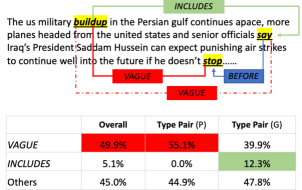
Figure 1: An example of the event temporal ordering task. Text input is taken from the news dataset in our experiments. Solid lines / arrows between two highlighted events show their gold temporal relations, e.g. say BEFORE stop and buildup INCLUDES say, and the dash line shows a wrong prediction, i.e., the VAGUE relation between buildup and say. In the table, Column Overall shows the relation distribution over the entire training corpus; Column Type Pair (P) shows the predicted relation distribution condition on the event pairs having types occurrence and reporting (such as buildup and say); Column Type Pair (G) shows the gold relation distribution condition on event pairs having the same types. Biased predictions of VAGUE relation between buildup and say can be partially corrected by using the gold event type-relation statistics in Column Type Pair (G).

Predicting event temporal relations is inherently challenging as it requires the system to understand each event’s beginning and end times. However, these time anchors are often hard to specify within a complicated context, even for humans. As a result, there is usually a large amount of VAGUE pairs (nearly 50% in the table of Figure 1) in an expert-annotated dataset, resulting in heavily class-imbalanced datasets. Moreover, expert annotations are often time-consuming to gather, so the sizes of existing datasets are relatively small. To cope with the class-imbalance problem and the small dataset issues, recent research efforts adopt hard constraint-enhanced deep learning methods and leverage pre-trained language models Ning et al. (2018c); Han et al. (2019b) and are able to establish reasonable baselines for the task.

The hard-constraints used in the SOTA systems can only be constructed when they are nearly 100% correct and hence make the knowledge adoption restrictive. Temporal relation transitivity is a frequently used hard constraint that requires if A BEFORE B and B BEFORE C, it must be that A BEFORE C. However, constraints are usually not deterministic in real-world applications. For example, a clinical treatment and test are more likely to happen AFTER a medical problem, but not always. Such probabilistic constraints cannot be encoded with the hard-constraints as in the previous systems.

Furthermore, deep neural models have biased predictions on dominant classes, which is particularly concerning given the small and biased datasets in event temporal extraction. For example, in Figure 1, an event pair headed and say (with relation INCLUDES) is incorrectly predicted as VAGUE (Column Type Pair (P)) by our baseline neural model, partially due to dominant percentage of VAGUE label (Column Overall), and partially due to the complexity of the context. Using the domain knowledge that headed and say have event types of occurrence and reporting, respectively, we can find a new label probability distribution (Type Pair (G)) for this pair. The probability mass allocated to VAGUE would decrease by 10% and increase by 7.2% for INCLUDES, which significantly increases the chance for a correct label prediction.

We propose to improve deep structured neural networks by incorporating domain knowledge such as corpus statistics in the model inference, and by solving the constrained inference problem using Lagrangian Relaxation. This framework allows us to benefit from the strong contextual understanding of pre-trained language models while optimizing model outputs based on probabilistic structured knowledge that previous deep models fail to consider. Experimental results demonstrate the effectiveness of this framework.

We summarize our contributions below:

• We formulate the incorporation of probabilistic knowledge as a constrained inference problem and use it to optimize the outcomes from strong neural models.

• Novel applications of Lagrangian Relaxation on end-to-end temporal relation extraction task with event-type and relation constraints.

• Our framework significantly outperforms baseline systems without knowledge adoption and achieves new SOTA results on two datasets in news and clinical domains.

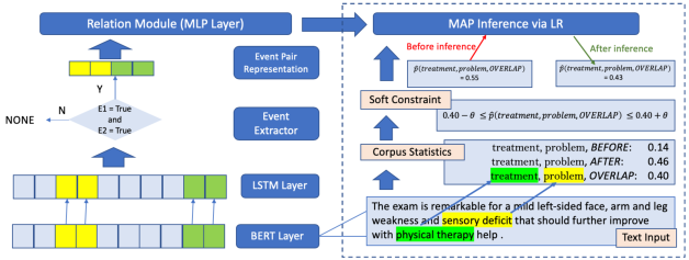
Figure 2: An overview of the proposed framework. The left column shows the end-to-end event temporal relation extraction workflow. The right column (in the dashed box) illustrates how we propose to enhance the end-to-end extraction system. The final MAP inference contains two components: scores from the relation module and distributional constraints constructed using domain knowledge and corpus statistics. The text input is a real example taken from the I2b2-Temporal dataset. The MAP inference is able to push the predicted probability of the event type-relation triplet closer to the ground-truth (corpus statistics).

2 Problem Formulation

The problem we focus on is end-to-end event temporal relation extraction, which takes a raw text as input, first identifies all events, and then classifies temporal relations for all predicted event pairs. The left column of Figure 2 shows an example. An end-to-end system is practical in a real-world setting where events are not annotated in the input and challenging because temporal relations are harder to predict after noise is introduced during event extraction.

3 Method

In this section, we first describe the details of our deep neural networks for an end-to-end event temporal relation extraction system, then show how to formulate domain-knowledge between event types and relations as distributional constraints in Integer Linear Programming (ILP), and finally apply Lagrangian Relaxation to solve the constrained inference problem. Our base model is trained end-to-end with cross-entropy loss and multitask learning to obtain relation scores. We need to perform an additional inference step in order to incorporate domain-knowledge as distributional constraints.

3.1 End-to-end Event Relation Extraction

As illustrated in the left column in Figure 2, our end-to-end model shares a similar work-flow as the pipeline model in Han et al. (2019b), where multi-task learning with a shared feature extractor is used to train the pipeline model. Let $\mathcal{E}$, $\mathcal{E}\mathcal{E}$ and $\mathcal{R}$ denote event, candidate event pairs and the feasible relations, respectively, in an input instance $\bm{x}^{n}$, where $n$ is the instance index. The combined training loss is $\mathcal{L}=c_{\mathcal{E}}\mathcal{L}_{\mathcal{E}}+\mathcal{L}_{\mathcal{R}}$, where $\mathcal{L}_{\mathcal{E}}$ and $\mathcal{L}_{\mathcal{R}}$ are the losses for the event extractor and the relation module, respectively, and $c_{\mathcal{E}}$ is a hyper-parameter balancing the two losses.

Feature Encoder.

Input instances are first sent to pre-trained language models such as BERT Devlin et al. (2018) and RoBERTa Liu et al. (2019), then to a Bi-LSTM layer as in previous event temporal relation extraction work Han et al. (2019a).

Encoded features will be used as inputs to the event extractor and the relation module below.

Event Extractor.

The event extractor first predicts scores over event classes for each input token and then detects event spans based on these scores. If an event has over more than one tokens, its beginning and ending vectors are concatenated as the final event representation. The event score is defined as the predicted probability distribution over event classes. Pairs predicted to include non-events are automatically labeled as NONE, whereas valid candidate event pairs are fed into the relation module to obtain their relation scores.

Relation Module.

The relation module’s input is a pair of events, which share the same encoded features as the event extractor. We simply concatenate them before feeding them into the relation module to produce relation scores $S(y^{r}_{i,j},\bm{x}^{n})$, which are computed using the Softmax function where $y^{r}_{i,j}$ is a binary indicator of whether an event pair $(i,j)\in\mathcal{E}\mathcal{E}$ has relation $r\in\mathcal{R}$.

3.2 Constrained Inference for Knowledge Incorporation

As shown in Figure  2, once the relation scores are computed via the relation module, a MAP inference is performed to incorporate distributional constraints so that the structured knowledge can be used to adjust neural baseline model scores and optimize the final model outputs. We formulate our MAP inference with distributional constraints as an LR problem and solve it with an iterative algorithm.

Next, we explain the details of each component in our MAP inference.

3.2.1 Distributional constraints

Much of the domain-knowledge required for real-world problems are probabilistic in nature. In the task of event relation extraction, domain-knowledge can be the prior probability of a specific event-pair’s occurrence acquired from large corpora or knowledge base Ning et al. (2018b); domain-knowledge can also be event-property and relation distribution obtained using corpus statistics, as we study in this work. Previous work mostly leverage hard constraints for inference (Yoshikawa et al., 2009; Ning et al., 2017; Leeuwenberg and Moens, 2017; Ning et al., 2018a; Han et al., 2019a, b), where constraints such as transitivity and event-relation consistency are assumed to be absolutely correct. As we discuss in Section 1, hard constraints are rigid and thus cannot be used to model probabilistic domain-knowledge.

The right column in Figure 2 illustrates how our work leverages corpus statistics to construct distributional constraints. Let $P$ be a set of event properties such as clinical types (e.g. treatment or problem).

For the pair $(P^{m},P^{n})$ and the triplet $(P^{m},P^{n},r)$, where $P^{n},P^{m}\in P$ and $r\in\mathcal{R}$, we can retrieve their counts in the training corpus as

$$C(P^{m},P^{n},r)=\sum_{i,j\in\mathcal{E}\mathcal{E}}c(P_{i}=P^{m};P_{j}=P^{n};r_{i,j}=r)$$

and

$$C(P^{m},P^{n})=\sum_{i,j\in\mathcal{E}\mathcal{E}}c(P_{i}=P^{m};P_{j}=P^{n}).$$

Let $t=(P^{m},P^{n},r)$. The prior triplet probability can thus be defined as

$$p^{*}_{t}= \frac{C(P^{m},P^{n},r)}{C(P^{m},P^{n})}.$$

Let $\hat{p}_{t}$ denote the predicted triplet probability, distributional constraints require that,

$$p^{*}_{t}-\theta\leq\hat{p}_{t}\leq p^{*}_{t}+\theta$$ (1)

where $\theta$ is the tolerance margin between the prior and predicted probabilities.

3.2.2 Integer Linear Programming with Distributional Constraints

We formulate our MAP inference as an ILP problem. Let $\mathcal{T}$ be a set of triplets whose predicted probabilities need to satisfy Equation 1. We can define our full ILP as

$$\mathcal{L}= \sum_{(i,j)\in\mathcal{E}\mathcal{E}}\sum_{r\in\mathcal{R}}y^{r}_{i,j}S(y^{r}_{i,j},\bm{x})$$ (2)

$$\textbf{s.t. }p^{*}_{t}-\theta\leq\hat{p}_{t}\leq p^{*}_{t}+\theta,\text{ }\forall t\in\mathcal{T}\text{, and}$$

$$y^{r}_{i,j}\in\{0,1\}\text{ , }\sum_{r\in\mathcal{R}}y^{r}_{i,j}=1,$$

where $S(y^{r}_{i,j},\bm{x}),\forall r\in\mathcal{R}$ is the scoring function obtained from the relation module. For $t=(P^{m},P^{n},r)$, we have $\hat{p}_{t}=\frac{\sum^{\mathcal{E}\mathcal{E}}_{(i:P^{m},j:P^{n})}y^{r}_{i,j}}{\sum^{\mathcal{E}\mathcal{E}}_{(i:P^{m},j:P^{n})}\sum_{r^{\prime}}^{\mathcal{R}}y^{r^{\prime}}_{i,j}}$. The output of the MAP inference, $\bf{\hat{y}}$, is a collection of optimal label assignments for all relation candidates in an input instance $\bm{x}^{n}$. $\sum_{r\in\mathcal{R}}y^{r}_{i,j}=1$ ensures that each event pair gets one label assignment and this is the only hard constraint we use.

To improve computational efficiency, we apply the heuristic to optimize only the equality constraints $p^{*}_{t}=\hat{p_{t}}$, $\forall t\in\mathcal{T}$. Our optimization algorithm terminates when $|p^{*}_{t}-\hat{p_{t}}|\leq\theta$. This heuristic has been shown to work efficiently without hurting inference performance (Meng et al., 2019). For each triplet $t$, its equality constraint can be rewritten as

$$F(t)=(1-p_{t}^{*})\sum^{\mathcal{E}\mathcal{E}}_{(i:P^{m},j:P^{n})}y^{r}_{i,j},$$ (3)

$$-p_{t}^{*}\sum^{\mathcal{E}\mathcal{E}}_{(i:P^{m},j:P^{n},}\sum^{\mathcal{R}}_{r^{\prime}\neq r)}y^{r^{\prime}}_{i,j} =0.$$

The goal is to maximize the objective function defined by Eq. (2) while satisfying the equality constraints.

Algorithm 1 Gradient Ascent for LR

1:procedure 

2:     for $t\in\mathcal{T}$ do

3:         $\lambda_{t}^{0}=0$      

4:     $k=0$

5:     while $k<K$ do $\triangleright$ $K$: max iteration

6:         $\hat{y}^{k+1}\leftarrow\arg\max\mathcal{L}(\bm{\lambda}^{k})$

7:         for $t\in\mathcal{T}$ do

8:              $\Delta_{t}=p^{*}_{t}-\hat{p}_{t}$

9:              if $|\Delta_{t}|>\theta$ then

10:                  $\lambda_{t}^{k+1}=\lambda_{t}^{k}+\alpha\Delta_{t}$                        

11:         if $\Delta_{t}\leq\theta,\forall t$ then

12:              break          

13:         $k=k+1$

14:         $\alpha=\gamma\alpha$ $\triangleright$ $\gamma$: decay rate      

3.2.3 Lagrangian Relaxation

Solving Eq. (2) is NP-hard. Thus, we reformulate it as a Lagrangian Relaxation problem by introducing Lagrangian multipliers $\lambda_{t}$ for each distributional constraint. Lagrangian Relaxation has been applied in a variety NLP tasks, as described by Rush and Collins (2011, 2012) and Zhao et al. (2017).

The Lagrangian Relaxation problem can be written as

$$\mathcal{L}(\mathbf{y},\bm{\lambda})= \sum_{(i,j)\in\mathcal{E}\mathcal{E}}\sum_{r\in\mathcal{R}}y^{r}_{i,j}S(y^{r}_{i,j},\bm{x})+\sum_{t\in\mathcal{T}}\lambda_{t}F(t).$$ (4)

Initialize $\lambda_{t}=0$. Eq. (4) can be solved with the following iterative algorithm (Algorithm 1).

1. At each iteration $k$, obtain the best relation assignments per MAP inference, $\hat{y}^{k}=\arg\max\mathcal{L}(\mathbf{y},\bm{\lambda})$

2. Update the Lagrangian multiplier in order to bring the predicted probability closer to the prior. Specifically, for each $t\in\mathcal{T}$,

   • If $|p^{*}_{t}-\hat{p}_{t}|\leq\theta$, $\lambda_{t}^{k+1}=\lambda_{t}^{k}$

   • Otherwise, $\lambda_{t}^{k+1}=\lambda_{t}^{k}+\alpha(p_{t}^{*}-\hat{p_{t}})$

$\alpha$ is the step size. We are solving a min-max problem: the first step chooses the maximum likelihood assignments by fixing $\bm{\lambda}$; the second step searches for $\bm{\lambda}$ values that minimize the objective function.

4 Constrained Inference Implementation

This section explains how to construct our distributional constraints and the implementation details for inference with LR.

Constraint Triplets	Count	$\%$
occurrence, occurrence, *	124	19.7
occurrence, reporting, *	50	7.9
occurrence, action, *	44	7.0
reporting, occurrence, *	41	6.5
action, occurrence, *	40	6.4
action, action, *	20	3.2
reporting, reporting, *	18	2.9
action, reporting, *	18	2.9
reporting, action, *	17	2.7

Table 1: TimeBank-Dense: triplet prediction count and percentage in the development set (sample size = 629).

	TimeBank-Dense				2012 i2b2 Challenge (I2b2-Temporal)
	Event	Relation			Event		Relation (TempEval Metrics)
	F1	R	P	F1	Span F1	Type Accuracy	R	P	F1
Feature-based Benchmark	87.4	43.8	35.7	39.4	90.1	86.0	37.8	51.8	43.0
Han et al. (2019b)	90.9	52.6	46.5	49.4	-	-	73.4	76.3	74.8
End-to-end Baseline	90.3	51.5	45.9	48.5	87.8	87.8	73.3	79.9	76.5
End-to-end + Inference	90.3	53.4	47.9	50.5	87.8	87.8	74.0	80.8	77.3

Table 2: Overall experiment results: per MacNemar’s test, the improvements against the end-to-end baseline models by adding inference with distributional constraints are both statistically significant for TimeBank-Dense (p-value $<0.005$) and I2b2-Temporal (p-value $<0.0005$). For I2b2-Temporal, our end-to-end system is optimized for the F₁ score of the gold pairs.

4.1 Distributional Constraint Selection

The selection of distributional constraints is crucial for our algorithm. If the probability of an event-type and relation triplet is unstable across different splits of data, we may over-correct the predicted probability. We use the following search algorithm with heuristic rules to ensure constraint stability.

4.1.1 TimeBank-Dense

For TimeBank-Dense, we first sort candidate constraints by their corresponding values of $C(P^{m},P^{n})=\sum_{\hat{r}\in\mathcal{R}}C(P^{m},P^{n},\hat{r})$. We list $C(P^{m},P^{n})$ with the largest prediction numbers and their percentages in the development set in Table 1.

Next, we set $3\%$ as our threshold to include constraints for our main experimental results. We found this number to work relatively well for both TimeBank-Dense and I2b2-Temporal. We will show the impact of relaxing this threshold in the discussion section. In Table 1, the constraints in the bottom block are filtered out. Moreover, Eq. 3 implies that a constraint defined on one triplet $(P^{m},P^{n},r)$ has impact on all $(P^{m},P^{n},r^{\prime})$ for $r^{\prime}\in\mathcal{R}\setminus r$. In other words, decreasing $\hat{p}_{(P^{m},P^{n},r)}$ is equivalent to increasing $\hat{p}_{(P^{m},P^{n},r^{\prime})}$ and vice versa. Thus, we heuristically pick $(P^{m},P^{n},{\textit{VAGUE}})$ as our default constraint triplets.

Finally, we adopt a greedy search rule to select the final set of constraints. We start with the top constraint triplet in Table 1 and then keep adding the next one as long as it doesn’t hurt the grid search F₁ score on the development set. Eventually, four constraints triplets are selected, and they can be found in Table 3.

4.1.2 I2b2-Temporal

Similar to TimeBank-Dense, we use the $3\%$ threshold to select candidate constraints. However, it is computationally expensive to use the greedy search rule above by conducting grid search as the number of constraints that pass this threshold is large (15 of them), development set sample size is more than 3 times of TimeBank-Dense, and a large transformer is used for modeling, Therefore, we incorporate another two heuristic rules to directly select constraints,

1. We randomly split the train data into five subsets of equal size $\{s_{1},s_{2},s_{3},s_{4},s_{5}\}$. For triplet $t$ to be selected, we must have $\frac{1}{5}\sum^{5}_{k=1}|p_{t,s_{k}}-p^{*}_{t}|<0.001$.

2. $|\hat{p}_{t}-p^{*}_{t}|>0.1$, where $\hat{p}_{t}$ is the predicted probability of $t$ on the development set.

The first rule ensures that a constraint triplet is stable over a randomly split of data; the second one ensures that the probability gaps between the predicted and gold are large so that we will not over-correct them. Eventually, four constraints satisfy these rules, and they can be found in Table 9, and we run only one final grid search for these constraints.

4.2 Inference

The ILP component in Sec. 3.2.2 is implemented using an off-the-shelf solver provided by Gurobi optimizer. Hyper-parameters choices can be found in Table 6 in the Appendix.

5 Experimental Setup

This section describes the two event temporal relation datasets used in this paper and then explains the evaluation metrics.

5.1 Data

TimeBank-Dense.

Temporal relation corpora such as TimeBank (Pustejovsky et al., 2003) and RED (O’Gorman et al., 2016) consist of expert annotations of news articles. The common issue of these corpora is missing annotations. Collecting densely annotated temporal relation corpora with all events and relations fully annotated is a challenging task as annotators could easily overlook some facts (Bethard et al., 2007; Cassidy et al., 2014; Chambers et al., 2014; Ning et al., 2017).

The TimeBank-Dense dataset mitigates this issue by forcing annotators to examine all pairs of events within the same or neighboring sentences, and this dataset has been widely evaluated on this task Chambers et al. (2014); Ning et al. (2017); Cheng and Miyao (2017); Meng and Rumshisky (2018). Temporal relations consist of BEFORE, AFTER, INCLUDES, INCLUDED, SIMULTANEOUS, and VAGUE. Moreover, each event has several properties, e.g., type, tense, and polarity. Event types include occurrence, action, reporting, state, etc. Event pairs that are more than 2 sentences away are not annotated.

I2b2-Temporal.

In the clinical domain, one of the earliest event temporal datasets was provided in the 2012 Informatics for Integrating Biology and the Bedside (i2b2) Challenge on NLP for Clinical Records Sun et al. (2013). Clinical events are categorized into 6 types: treatment, problem, test, clinical-dept, occurrence, and evidential. The final data used in the challenge contains three temporal relations: BEFORE, AFTER, and OVERLAP. The 2012 i2b2 challenge also had an end-to-end track, which we use as our feature-based system baseline. To mimic the input structure of TimeBank-Dense, we only consider event pairs that are within 3 consecutive sentences. Overall, 13% of the long-distance relations are excluded.

5.2 Evaluation Metrics

To be consistent with previous work, we adopt two different evaluation metrics. For TimeBank-Dense, we use standard micro-average scores that are also used in the baseline system Han et al. (2019b). Since the end-to-end system can predict the gold pair as NONE, we follow the convention of IE tasks and exclude them from the evaluation. For I2b2-Temporal, we adopt the TempEval evaluation metrics used in the 2012 i2b2 challenge. These evaluation metrics differ from the standard F₁ in a way that it computes the graph closure for both gold and predictions labels. Since I2b2-Temporal contains roughly six times more missing annotations than the gold pairs, we only evaluate the performance of the gold pairs.

Both datasets contain three types of entities: events, time expressions, and document time. In this work, we focus on event-event relations and exclude all other relations from the evaluation.

5.3 Baselines

Feature-based Systems.

We use CAEVO (Chambers et al., 2014), a hybrid system of rules and linguistic feature-based MaxEnt classifier, as our feature-based benchmark for TimeBank-Dense. Model implementation and performance are both provided by Han et al. (2019b). As for I2b2-Temporal, we retrieve the predictions from the top end-to-end system provided by Yan et al. (2013) and report the performance according to the evaluation metrics specified in Section 5.2.

Neural Model Baselines.

We use the end-to-end systems described by Han et al. (2019b) as our neural network model benchmarks (Row 2 of Table 2). For TimeBank-Dense, the best global structured model’s performance is reported by Han et al. (2019b). For I2b2-Temporal, we re-implement the pipeline joint model. Note that this end-to-end model only predicts whether each token is an event as well as each pair of token’s relation. Event spans are not predicted, so head-tokens are used to represent events; event types are also not predicted. Therefore, we do not report Span F₁ and Type Accuracy in this benchmark.

End-to-end Baseline.

For the TimeBank-Dense dataset, we use the pipeline joint (local) model with no global constraints as presented by Han et al. (2019b). In contrast to the aforementioned neural baseline provided in the same paper, this end-to-end model does not use any inference techniques. Hence, it serves as a fair baseline for our method (with inference). For TimeBank-Dense, we build our framework based on this model.

For the I2b2-Temporal dataset to be more comparable with the 2012 i2b2 challenge, we augment the event extractor illustrated in Figure 2 by allowing event type predictions; that is, for each input token, we not only predict whether it is an event or not, but also predict its event type. We follow the convention in the IE field by adding a “BIO” label to each token in the data. For example, the two tokens in “physical therapy” in Figure 2 will be labeled as B-treatment and I-treatment, respectively. To be consistent with the partial match method used in the 2012 i2b2 challenge, the event span detector looks for token predictions that start with either “B-” or “I-” and ensures that all tokens predicted within the same event span have only one event type.

RoBERTa-large is used as the base model, and cross-entropy loss is used to train the model. We fine-tune the base model and conduct a grid search on the random hold-out set to pick the best hyper-parameters such as $c_{\mathcal{E}}$ in the multitask learning loss and the weight, $w_{\mathcal{E}_{pos}}$ for positive event types (i.e. B- and I-). The best hyper-parameter choices can be found in Table 6 in the Appendix.

6 Results and Analysis

Table 2 contains our main results. We discuss model performances on TimeBank-Dense and I2b2-Temporal in this section.

6.1 TimeBank-Dense

All neural models outperform the feature-based system by more than 10% per relation F₁ score. Our structured model outperforms the previous SOTA systems with hard constraints and joint event and relation training by 1.1%. Compared with the end-to-end baseline model with no constraints, our system achieves 2% absolute improvement, which is statistically significant with a $p$-value $<0.005$ per MacNemar’s test. This is strong evidence that leveraging Lagrangian Relaxation to incorporate domain knowledge can be extremely beneficial even for strong neural network models.

The ablation study in Table 3 shows how distributional constraints work and the constraints’ individual contributions. The predicted probability gaps shrink by 0.15, 0.24, and 0.13 respectively for the three constraints chosen, while providing 0.91%, 0.65%, and 0.44% improvements to the final F₁ score for relation extraction. We also show the breakdown of the performance for each relation class in Table 4. The overall F₁ improvement is mainly driven by the recall scores in the positive relation classes (BEFORE, AFTER, and INCLUDES) that have much smaller sample size than VAGUE. These results are consistent with the ablation study in Table 3, where the end-to-end baseline model over-predicts on VAGUE, and the LR algorithm corrects it by assigning less confident predictions on VAGUE to positive and minority classes according to their relation scores.

6.2 I2b2-Temporal

All neural models outperform the feature-based system by more than 30% per relation F₁ score. Our structured model with distributional constraints outperforms the neural pipeline joint models of Han et al. (2019b) by 2.5% per absolute scale. Compared with our end-to-end baseline model, our system achieves 0.77% absolute improvement on F₁ measure, which is statistically significant with a $p$-value $<0.0005$ per MacNemar’s test. This result also shows that adding inference with distributional constraints can be helpful for strong neural baseline models.

Table 9 in the Appendix Section C shows how distributional constraints work and their individual contributions. Predicted probability gaps shrink by 0.17, 0.16, 0.11, and 0.14, respectively, for the four constraints chosen, providing 0.19%, 0.25%, 0.22%, and 0.12% improvements to the final F₁ scores for relation extraction. We also have the breakdown performance for each relation class in Table 8. The performance gain is caused mostly by the increase of recall scores in BEFORE and AFTER. This is consistent with the results in Table 9 where the model over-predicts on the OVERLAP class, possibly because of label imbalance. Inference is able to partially correct this mistake by leveraging distributional constraints constructed with event type and relation corpus statistics.

Constraint Triplets	Prob. Gap	F1
occur., occur., VAGUE	-0.15	+0.91%
occur., reporting, VAGUE	-0.24	+0.65%
action, occur., VAGUE	-0.13	+0.44%
reporting, occur., VAGUE∗	0.0	0%
Combined F1 Improvement		2.0%

Table 3: TimeBank-Dense ablation study: gap shrinkage of predicted probability and F₁ contribution per constraint. ^∗ is selected per Sec. 4, but the probability gap is smaller than the tolerance in the test set, hence no impact to the F₁ score.

	End-to-end Baseline			End-to-end Inference
	P	R	F1	P	R	F1
B	59.0	46.9	52.3	58.6	55.7	57.1
A	69.3	45.3	54.8	67.8	51.5	58.5
I	-	-	-	8.3	1.8	2.9
II	-	-	-	-	-	-
S	-	-	-	-	-	-
V	45.1	55.0	49.5	47.6	51.4	49.4
Avg	51.5	45.9	48.5	53.4	47.9	50.5

Table 4: Model performance breakdown for TimeBank-Dense. “-” indicates no predictions were made for that particular label, probably due to the small size of the training sample. BEFORE (B), AFTER (A), INCLUDES (I), IS_INCLUDED (II), SIMULTANEOUS (S), VAGUE (V)

6.3 Qualitative Error Analysis

We can use the errors made by our structured neural model on TimeBank-Dense to guide potential directions for future research. There are 26 errors made by the structured model that are correctly predicted by the baseline model. In Table 5, we show the error breakdown by constraints. Our method works by leveraging corpus statistics to correct borderline errors made by the baseline model; however, when the baseline model makes borderline correct predictions, the inference could mistakenly change them to the wrong labels. This situation can happen when the context is complicated or when the event time interval is confusing.

For the constraint (occur., occur., VAGUE), nearly all errors are cross-sentence event pairs with long context information. In ex.1, the gold relation between responded and use is VAGUE because of the negation of use, but one could also argue that if use were to happen, responded is BEFORE use. This inherent annotation confusion can cause the baseline model to predict VAGUE marginally over BEFORE. When informed by the constraint statistics that vague is over-predicted, the inference algorithm revises the baseline prediction to BEFORE. Similarly, in ex.2 and ex.3, one could make strong cases that both the relations between delving and acknowledged, and opposed and expansion are BEFORE rather than VAGUE from the context. This annotation ambiguity can contribute to the errors made by the proposed method.

Our analysis shows that besides the necessity to create high-quality data for event temporal relation extraction, it could be useful to incorporate additional information such as discourse relation (particularly for (occur., occur., VAGUE)) and other prior knowledge on event properties to resolve the ambiguity in event temporal reasoning.

occurrence, occurrence, VAGUE (57.7%)

ex.1 In a bit of television diplomacy, Iraq’s deputy

foreign minister responded from Baghdad in less than

one hour, saying Washington would break international

law by attacking without UN approval. The United States

is not authorized to use force before going to the council.

occurrence, reporting, VAGUE (26.9%)

ex.2 A new Essex County task force began delving

Thursday into the slayings of 14 black women over the

last five years in the Newark area, as law-enforcement

officials acknowledged that they needed to work harder…

action, occurrence, VAGUE (15.4%)

ex.3 The Russian leadership has staunchly opposed

the western alliance’s expansion into Eastern Europe.

Table 5: Error examples and breakdown by constraints.

7 Discussion

7.1 Constraint Selection

In Sec. 4, we use a 3% threshold when selecting candidate constraints. In this section, we show the impact of relaxing this threshold on TimeBank-Dense. Table 1 shows three constraints that miss the 3% bar by 0.1-0.3%. In Figure 3, we show F₁ scores on the development and test sets by including these constraints. Recall that only constraints that do not hurt development F₁ score are used. Therefore, Top5 and Top6 on the chart both correspond to the results in Table 2. Top7 includes (reporting, reporting, VAGUE), Top8 includes (actioin, reporting, VAGUE), and Top9 includes (reporting, actioin, VAGUE).

We observe that F₁ score continues to improve over the development set, but on the test set, F₁ score eventually falls. This appears to support our hypothesis that when the triplet count is small, the ratio calculated based on that count is not so reliable as the ratio could vary drastically between development and test sets. Optimizing over the development set can be an over-correction for the test set, and hence results in a performance drop.

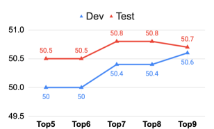
Figure 3: Dev v.s. Test sets performance ($F_{1}$ score) after relaxing the threshold of triplet count for selecting constraints. All numbers are percentages.

7.2 Event Type Prediction

As described in Sec 5.3, to ensure fair comparison with the previous SOTA system Han et al. (2019b), our baseline model for TimeBank-Dense does not predict event types. That is, when counting the triplet $(P^{m},P^{n},\hat{r})$, we assume there is an oracle model that provides event types $P^{m},P^{n}$ for the predicted relation $\hat{r}$. One could potentially extend our work by training a similar multi-task learning model to predict both types and relations as our model does for the I2b2-Temporal dataset. We leave this as a future research direction.

8 Related Work

News Domain.

Early work on temporal relation extraction use local pair-wise classification with hand-engineered features Mani et al. (2006); Verhagen et al. (2007); Chambers et al. (2007); Verhagen and Pustejovsky (2008). Later efforts, such as ClearTK (Bethard, 2013), UTTime (Laokulrat et al., 2013), NavyTime Chambers (2013), and CAEVO (Chambers et al., 2014), improve earlier work with better linguistic and syntactic rules. Yoshikawa et al. (2009); Ning et al. (2017); Leeuwenberg and Moens (2017) explore structured learning for this task, and more recently, neural methods have also been shown effective Tourille et al. (2017); Cheng and Miyao (2017); Meng et al. (2017); Meng and Rumshisky (2018). Ning et al. (2018c) and Han et al. (2019b) are the most recent work leveraging neural network and pre-trained language models to build an end-to-end system. Our work differs from these prior work in that we build a structured neural model with distributional constraints that combines both the benefits of both deep learning and domain knowledge.

Clinical Domain.

The 2012 i2b2 Challenge (Sun et al. (2013)) is one of the earliest efforts to advance event temporal relation extraction of clinical data. The challenge hosted three tasks on event (and event property) classification, temporal relation extraction, and the end-to-end track. Following this early effort, a series of clinical event temporal relation challenges were created in the following years (Bethard et al. (2015, 2016, 2017)). However, data in these challenges are relatively hard to acquire, and therefore they are not used in this paper. As in the news data, traditional machine learning approaches Lee et al. (2016); Chikka (2016); Xu et al. (2013); Tang et al. (2013); Savova et al. (2010) that tackle the end-to-end event and temporal relation extraction problem require time-consuming feature engineering such as collecting lexical and syntax features. Some recent work Dligach et al. (2017); Leeuwenberg and Moens (2017); Galvan et al. (2018) apply neural network-based methods to model the temporal relations, but are not capable of incorporating prior knowledge about clinical events and temporal relations as proposed by our framework.

9 Conclusion

In conclusion, we propose a general framework that augments deep neural networks with distributional constraints constructed using probabilistic domain knowledge. We apply it in the setting of end-to-end temporal relation extraction task with event-type and relation constraints and show that the MAP inference with distributional constraints can significantly improve the final results.

We plan to apply the proposed framework on various event reasoning tasks and construct novel distributional constraints that could leverage domain knowledge beyond corpus statistics, such as the larger unlabeled data and rich information contained in knowledge bases.

Appendix

Appendix A Hyper-parameters

	TimeBank-Dense	I2b2-Temporal
$c_{\mathcal{E}}$	-	1.0
$w_{\mathcal{E}_{pos}}$	-	5.0
lr	-	$2e^{-5}$
$\alpha$	5.0	5.0
$\theta$	0.05	0.02
$\gamma$	0.7	0.8

Table 6: Hyper-parameters chosen using development data. For TimeBank-Dense, end-to-end baseline model is provided by the Han et al. (2019b), so we do not train it from scratch.

Appendix B Data Summary

	TimeBank-Dense	I2b2-Temporal
# of Documents
Train	22	190
Dev	5	-
Test	9	120
# of Pairs
Train	4032	11253
Dev	629	-
Test	1427	8794

Table 7: Data overview. Note that we exclude event pairs whose sentence distance longer than 3 in I2b2-Temporal, and there are 6 times more missing relations than the gold annotated ones in, which explains why number of pairs per documents are smaller in I2b2-Temporal than in TimeBank-Dense.

Appendix C I2b2-Temporal Results

We show the breakdown performance and contributions of individual constraints for I2b2-Temporal in Table 8 and Table 9 respectively.

	End-to-end Baseline			End-to-end Inference
	P	R	F1	P	R	F1
B	82.1	60.6	69.7	80.9	65.3	72.2
A	69.9	59.9	64.5	67.8	62.8	65.2
O	81.3	81.5	81.4	83.6	80.2	81.9
TempEval	73.3	79.9	76.5	74.0	80.8	77.3

Table 8: Model performance breakdown for I2b2-Temporal. BEFORE (B), AFTER (A), OVERLAP (O).

Constraint Triplets	Prob. Gap	F1
occur., problem, OVERLAP	-0.17	+0.19%
occur., treatment, OVERLAP	-0.16	+0.24%
treatment, occur., OVERLAP	-0.11	+0.22%
treatment, problem, OVERLAP	-0.14	+0.12%
Combined F1 Improvement		0.77%

Table 9: I2b2-Temporal ablation study: gap shrinkage of predicted probability and F₁ contribution per constraint.

Appendix D Reproducibility List

• Data and code used for TimeBank-Dense can be found in project code base. However, due to user confidentiality agreement, we are not able to provide data and and data analysis code for I2b2-Temporal. Modeling code will be added to the project code base upon obtaining permission from the data owner.

• We use BERT-base-uncased and Roberta-large models implemented in Huggingface transformers. Additional parameters (such as LSTM and MLP) are negligible compared to those used in the pre-trained LMs;

• ILP is solved by an off-the-shelf solver provided by Gurobi optimizer;

• Range of grid-search. $c_{\mathcal{E}}$: (1.0, 2.0); $w_{\mathcal{E}_{pos}}$: (1.0, 2.0, 5.0, 10.0); lr: ($1e^{-5}$, $2e^{-5}$, $5e^{-5}$), $\alpha$: (1.0, 2.0, 5.0, 10.0); $\theta$: (0.2, 0.3, 0.5); $\gamma$: (0.7, 0.8, 0.9).

References

- Bethard (2013) Steven Bethard. 2013. Cleartk-timeml: A minimalist approach to tempeval 2013. In Second Joint Conference on Lexical and Computational Semantics (*SEM), Volume 2: Proceedings of the Seventh International Workshop on Semantic Evaluation (SemEval 2013), pages 10–14. Association for Computational Linguistics.
- Bethard et al. (2015) Steven Bethard, Leon Derczynski, Guergana Savova, James Pustejovsky, and Marc Verhagen. 2015. SemEval-2015 task 6: Clinical TempEval. In Proceedings of the 9th International Workshop on Semantic Evaluation (SemEval 2015), pages 806–814, Denver, Colorado. Association for Computational Linguistics.
- Bethard et al. (2007) Steven Bethard, James H. Martin, and Sara Klingenstein. 2007. Timelines from text: Identification of syntactic temporal relations. In Proceedings of the International Conference on Semantic Computing, ICSC ’07, pages 11–18, Washington, DC, USA. IEEE Computer Society.
- Bethard et al. (2016) Steven Bethard, Guergana Savova, Wei-Te Chen, Leon Derczynski, James Pustejovsky, and Marc Verhagen. 2016. SemEval-2016 task 12: Clinical TempEval. In Proceedings of the 10th International Workshop on Semantic Evaluation (SemEval-2016), pages 1052–1062, San Diego, California. Association for Computational Linguistics.
- Bethard et al. (2017) Steven Bethard, Guergana Savova, Martha Palmer, and James Pustejovsky. 2017. SemEval-2017 task 12: Clinical TempEval. In Proceedings of the 11th International Workshop on Semantic Evaluation (SemEval-2017), pages 565–572, Vancouver, Canada. Association for Computational Linguistics.
- Cassidy et al. (2014) Taylor Cassidy, Bill McDowell, Nathanael Chambers, and Steven Bethard. 2014. An annotation framework for dense event ordering. In Proceedings of the 52nd Annual Meeting of the Association for Computational Linguistics (Volume 2: Short Papers), pages 501–506. Association for Computational Linguistics.
- Chambers (2013) Nate Chambers. 2013. Navytime: Event and time ordering from raw text. In Second Joint Conference on Lexical and Computational Semantics (*SEM), Volume 2: Proceedings of the Seventh International Workshop on Semantic Evaluation (SemEval 2013), pages 73–77, Atlanta, Georgia, USA. Association for Computational Linguistics.
- Chambers et al. (2014) Nathanael Chambers, Taylor Cassidy, Bill McDowell, and Steven Bethard. 2014. Dense event ordering with a multi-pass architecture. In ACL.
- Chambers et al. (2007) Nathanael Chambers, Shan Wang, and Dan Jurafsky. 2007. Classifying temporal relations between events. In Proceedings of the 45th Annual Meeting of the ACL on Interactive Poster and Demonstration Sessions, ACL ’07, pages 173–176, Stroudsburg, PA, USA. Association for Computational Linguistics.
- Cheng and Miyao (2017) Fei Cheng and Yusuke Miyao. 2017. Classifying temporal relations by bidirectional lstm over dependency paths. In Proceedings of the 55th Annual Meeting of the Association for Computational Linguistics (Volume 2: Short Papers), volume 2, pages 1–6.
- Chikka (2016) Veera Raghavendra Chikka. 2016. CDE-IIITH at SemEval-2016 task 12: Extraction of temporal information from clinical documents using machine learning techniques. In Proceedings of the 10th International Workshop on Semantic Evaluation (SemEval-2016), pages 1237–1240, San Diego, California. Association for Computational Linguistics.
- Devlin et al. (2018) Jacob Devlin, Ming-Wei Chang, Kenton Lee, and Kristina Toutanova. 2018. Bert: Pre-training of deep bidirectional transformers for language understanding. In NAACL-HLT.
- Dligach et al. (2017) Dmitriy Dligach, Timothy Miller, Chen Lin, Steven Bethard, and Guergana Savova. 2017. Neural temporal relation extraction. In Proceedings of the 15th Conference of the European Chapter of the Association for Computational Linguistics: Volume 2, Short Papers, pages 746–751, Valencia, Spain. Association for Computational Linguistics.
- Galvan et al. (2018) Diana Galvan, Naoaki Okazaki, Koji Matsuda, and Kentaro Inui. 2018. Investigating the challenges of temporal relation extraction from clinical text. In Proceedings of the Ninth International Workshop on Health Text Mining and Information Analysis, pages 55–64, Brussels, Belgium. Association for Computational Linguistics.
- Han et al. (2019a) Rujun Han, I-Hung Hsu, Mu Yang, Aram Galstyan, Ralph Weischedel, and Nanyun Peng. 2019a. Deep structured neural network for event temporal relation extraction. In Proceedings of the 23rd Conference on Computational Natural Language Learning (CoNLL), pages 666–106, Hong Kong, China. Association for Computational Linguistics.
- Han et al. (2019b) Rujun Han, Qiang Ning, and Nanyun Peng. 2019b. Joint event and temporal relation extraction with shared representations and structured prediction. In Proceedings of the 2019 Conference on Empirical Methods in Natural Language Processing and the 9th International Joint Conference on Natural Language Processing (EMNLP-IJCNLP), pages 434–444, Hong Kong, China. Association for Computational Linguistics.
- Laokulrat et al. (2013) Natsuda Laokulrat, Makoto Miwa, Yoshimasa Tsuruoka, and Takashi Chikayama. 2013. Uttime: Temporal relation classification using deep syntactic features. In Second Joint Conference on Lexical and Computational Semantics (*SEM), Volume 2: Proceedings of the Seventh International Workshop on Semantic Evaluation (SemEval 2013), pages 88–92, Atlanta, Georgia, USA. Association for Computational Linguistics.
- Lee et al. (2016) Hee-Jin Lee, Hua Xu, Jingqi Wang, Yaoyun Zhang, Sungrim Moon, Jun Xu, and Yonghui Wu. 2016. UTHealth at SemEval-2016 task 12: an end-to-end system for temporal information extraction from clinical notes. In Proceedings of the 10th International Workshop on Semantic Evaluation (SemEval-2016), pages 1292–1297, San Diego, California. Association for Computational Linguistics.
- Leeuwenberg and Moens (2017) Artuur Leeuwenberg and Marie-Francine Moens. 2017. Structured learning for temporal relation extraction from clinical records. In Proceedings of the 15th Conference of the European Chapter of the Association for Computational Linguistics: Volume 1, Long Papers, volume 1, pages 1150–1158.
- Liu et al. (2019) Yinhan Liu, Myle Ott, Naman Goyal, Jingfei Du, Mandar Joshi, Danqi Chen, Omer Levy, Mike Lewis, Luke Zettlemoyer, and Veselin Stoyanov. 2019. Roberta: A robustly optimized bert pretraining approach. arXiv preprint, arXiv:1907.11692.
- Mani et al. (2006) Inderjeet Mani, Marc Verhagen, Ben Wellner, Chong Min Lee, and James Pustejovsky. 2006. Machine learning of temporal relations. In Proceedings of the 21st International Conference on Computational Linguistics and the 44th Annual Meeting of the Association for Computational Linguistics, ACL-44, pages 753–760, Stroudsburg, PA, USA. Association for Computational Linguistics.
- Meng et al. (2019) Tao Meng, Nanyun Peng, and Kai-Wei Chang. 2019. Target language-aware constrained inference for cross-lingual dependency parsing. In Proceedings of the 2019 Conference on Empirical Methods in Natural Language Processing and the 9th International Joint Conference on Natural Language Processing (EMNLP-IJCNLP), pages 1117–1128, Hong Kong, China. Association for Computational Linguistics.
- Meng and Rumshisky (2018) Yuanliang Meng and Anna Rumshisky. 2018. Context-aware neural model for temporal information extraction. In Proceedings of the 56th Annual Meeting of the Association for Computational Linguistics (Volume 1: Long Papers).
- Meng et al. (2017) Yuanliang Meng, Anna Rumshisky, and Alexey Romanov. 2017. Temporal information extraction for question answering using syntactic dependencies in an lstm-based architecture. In Proceedings of the 2017 Conference on Empirical Methods in Natural Language Processing, pages 887–896.
- Ning et al. (2017) Qiang Ning, Zhili Feng, and Dan Roth. 2017. A structured learning approach to temporal relation extraction. In EMNLP, Copenhagen, Denmark.
- Ning et al. (2018a) Qiang Ning, Zhili Feng, Hao Wu, and Dan Roth. 2018a. Joint reasoning for temporal and causal relations. In Proceedings of the 56th Annual Meeting of the Association for Computational Linguistics (Volume 1: Long Papers), pages 2278–2288. Association for Computational Linguistics.
- Ning et al. (2018b) Qiang Ning, Hao Wu, Haoruo Peng, and Dan Roth. 2018b. Improving temporal relation extraction with a globally acquired statistical resource. In Proceedings of the 2018 Conference of the North American Chapter of the Association for Computational Linguistics: Human Language Technologies, Volume 1 (Long Papers), pages 841–851, New Orleans, Louisiana. Association for Computational Linguistics.
- Ning et al. (2018c) Qiang Ning, Ben Zhou, Zhili Feng, Haoruo Peng, and Dan Roth. 2018c. CogCompTime: A tool for understanding time in natural language. In Proceedings of the 2018 Conference on Empirical Methods in Natural Language Processing: System Demonstrations, pages 72–77, Brussels, Belgium. Association for Computational Linguistics.
- O’Gorman et al. (2016) Tim O’Gorman, Kristin Wright-Bettner, and Martha Palmer. 2016. Richer event description: Integrating event coreference with temporal, causal and bridging annotation. In Proceedings of 2nd Workshop on Computing News Storylines, pages 47–56. Association for Computational Linguistics.
- Pustejovsky et al. (2003) James Pustejovsky, Patrick Hanks, Roser Sauri, Andrew See, Robert Gaizauskas, Andrea Setzer, Dragomir Radev, Beth Sundheim, David Day, and Lisa Ferro. 2003. The timebank corpus. In Corpus linguistics, pages 647–656.
- Rush and Collins (2011) Alexander M. Rush and Michael Collins. 2011. Exact decoding of syntactic translation models through Lagrangian relaxation. In Proceedings of the 49th Annual Meeting of the Association for Computational Linguistics: Human Language Technologies, pages 72–82, Portland, Oregon, USA. Association for Computational Linguistics.
- Rush and Collins (2012) Alexander M Rush and MJ Collins. 2012. A tutorial on dual decomposition and lagrangian relaxation for inference in natural language processing. Journal of Artificial Intelligence Research, page 305–362.
- Savova et al. (2010) Guergana K Savova, James J Masanz, Philip V Ogren, Jiaping Zheng, Sunghwan Sohn, Karin C Kipper-Schuler, and Christopher G Chute. 2010. Mayo clinical text analysis and knowledge extraction system (ctakes): architecture, component evaluation and applications. Journal of the American Medical Informatics Association, 17(5):507–513.
- Sun et al. (2013) Weiyi Sun, Anna Rumshisky, and Ozlem Uzuner. 2013. Evaluating temporal relations in clinical text: 2012 i2b2 challenge.
- Tang et al. (2013) Buzhou Tang, Yonghui Wu, Min Jiang, Yukun Chen, Joshua C Denny, and Hua Xu. 2013. A hybrid system for temporal information extraction from clinical text. Journal of the American Medical Informatics Association, 20(5):828–835.
- Tourille et al. (2017) Julien Tourille, Olivier Ferret, Aurelie Neveol, and Xavier Tannier. 2017. Neural architecture for temporal relation extraction: a bi-lstm approach for detecting narrative containers. In Proceedings of the 55th Annual Meeting of the Association for Computational Linguistics (Volume 2: Short Papers), volume 2, pages 224–230.
- Verhagen et al. (2007) Marc Verhagen, Robert Gaizauskas, Frank Schilder, Mark Hepple, Graham Katz, and James Pustejovsky. 2007. Semeval-2007 task 15: Tempeval temporal relation identification. In Proceedings of the 4th International Workshop on Semantic Evaluations, SemEval ’07, pages 75–80, Stroudsburg, PA, USA. Association for Computational Linguistics.
- Verhagen and Pustejovsky (2008) Marc Verhagen and James Pustejovsky. 2008. Temporal processing with the tarsqi toolkit. In 22Nd International Conference on on Computational Linguistics: Demonstration Papers, COLING ’08, pages 189–192, Stroudsburg, PA, USA. Association for Computational Linguistics.
- Xu et al. (2013) Yan Xu, Yining Wang, Tianren Liu, Junichi Tsujii, and Eric I-Chao Chang. 2013. An end-to-end system to identify temporal relation in discharge summaries: 2012 i2b2 challenge. Journal of the American Medical Informatics Association, 20(5):849–858.
- Yan et al. (2013) Xu Yan, Wang Yining, Liu Tianren, Tsujii Junichi, and Chang EI. 2013. An end-to-end system to identify temporal relation in discharge summaries: 2012 i2b2 challenge.
- Yoshikawa et al. (2009) Katsumasa Yoshikawa, Sebastian Riedel, Masayuki Asahara, and Yuji Matsumoto. 2009. Jointly identifying temporal relations with markov logic. In Proceedings of the Joint Conference of the 47th Annual Meeting of the ACL and the 4th International Joint Conference on Natural Language Processing of the AFNLP: Volume 1-Volume 1, pages 405–413. Association for Computational Linguistics.
- Zhao et al. (2017) Jieyu Zhao, Tianlu Wang, Mark Yatskar, Vicente Ordonez, and Kai-Wei Chang. 2017. Men also like shopping: Reducing gender bias amplification using corpus-level constraints. In Proceedings of the 2017 Conference on Empirical Methods in Natural Language Processing, pages 2979–2989, Copenhagen, Denmark. Association for Computational Linguistics.