Cosmological 3D Hi Gas Map with HETDEX Ly $\alpha$ Emitters and eBOSS QSOs at $z=2$ :
IGM-Galaxy/QSO Connection and a $\sim$ 40-Mpc Scale Giant Hii Bubble Candidate

Shiro Mukae Institute for Cosmic Ray Research, The University of Tokyo, 5-1-5 Kashiwanoha, Kashiwa, Chiba 277-8582, Japan Department of Astronomy, Graduate School of Science, The University of Tokyo, 7-3-1 Hongo, Bunkyo, Tokyo, 113-0033, Japan mukae@icrr.u-tokyo.ac.jp Masami Ouchi National Astronomical Observatory of Japan, 2-21-1 Osawa, Mitaka, Tokyo 181-8588, Japan Institute for Cosmic Ray Research, The University of Tokyo, 5-1-5 Kashiwanoha, Kashiwa, Chiba 277-8582, Japan Kavli Institute for the Physics and Mathematics of the Universe (Kavli IPMU, WPI), The University of Tokyo, 5-1-5 Kashiwanoha, Kashiwa, Chiba, 277-8583, Japan Gary J. Hill Department of Astronomy, The University of Texas at Austin, 2515 Speedway, Stop C1400, Austin, Texas 78712, USA McDonald Observatory, University of Texas at Austin, 2515 Speedway, Stop C1402, Austin, TX 78712, USA Karl Gebhardt Department of Astronomy, The University of Texas at Austin, 2515 Speedway, Stop C1400, Austin, Texas 78712, USA Erin Mentuch Cooper Department of Astronomy, The University of Texas at Austin, 2515 Speedway, Stop C1400, Austin, Texas 78712, USA Donghui Jeong Department of Astronomy and Astrophysics, The Pennsylvania State University, University Park, PA 16802 Institute for Gravitation and the Cosmos, The Pennsylvania State University, University Park, PA 16802 Shun Saito Institute for Multi-messenger Astrophysics and Cosmology, Department of Physics, Missouri University of Science and Technology, 1315 N. Pine Street, Rolla, MO 65409, USA Kavli Institute for the Physics and Mathematics of the Universe (Kavli IPMU, WPI), The University of Tokyo, 5-1-5 Kashiwanoha, Kashiwa, Chiba, 277-8583, Japan Maximilian Fabricius Max-Planck-Institut für extraterrestrische Physik, Giessenbachstrasse, D-85748 Garching, Germany Universitäts-Sternwarte München, Scheinerstrasse 1, D-81679 München, Germany Eric Gawiser Department of Physics and Astronomy, Rutgers University, Piscataway, NJ 08854, USA Robin Ciardullo Department of Astronomy and Astrophysics, The Pennsylvania State University, University Park, PA 16802 Institute for Gravitation and the Cosmos, The Pennsylvania State University, University Park, PA 16802 Daniel Farrow Max-Planck-Institut für extraterrestrische Physik, Giessenbachstrasse, D-85748 Garching, Germany Dustin Davis Department of Astronomy, The University of Texas at Austin, 2515 Speedway, Stop C1400, Austin, Texas 78712, USA Greg Zeimann Hobby Eberly Telescope, University of Texas, Austin, TX 78712, USA Steven L. Finkelstein Department of Astronomy, The University of Texas at Austin, 2515 Speedway, Stop C1400, Austin, Texas 78712, USA Caryl Gronwall Department of Astronomy and Astrophysics, The Pennsylvania State University, University Park, PA 16802 Institute for Gravitation and the Cosmos, The Pennsylvania State University, University Park, PA 16802 Chenxu Liu Department of Astronomy, The University of Texas at Austin, 2515 Speedway, Stop C1400, Austin, Texas 78712, USA Yechi Zhang Institute for Cosmic Ray Research, The University of Tokyo, 5-1-5 Kashiwanoha, Kashiwa, Chiba 277-8582, Japan Department of Astronomy, Graduate School of Science, The University of Tokyo, 7-3-1 Hongo, Bunkyo, Tokyo, 113-0033, Japan Chris Byrohl Max-Planck-Institut für Astrophysik, Karl-Schwarzschild-Str. 1, D-85748 Garching, Germany Yoshiaki Ono Institute for Cosmic Ray Research, The University of Tokyo, 5-1-5 Kashiwanoha, Kashiwa, Chiba 277-8582, Japan Donald P. Schneider Department of Astronomy and Astrophysics, The Pennsylvania State University, University Park, PA 16802 Institute for Gravitation and the Cosmos, The Pennsylvania State University, University Park, PA 16802 Matt J. Jarvis Astrophysics, Department of Physics, Keble Road, Oxford, OX1 3RH, UK Department of Physics & Astronomy, University of the WesternCape, Private Bag X17, Bellville, Cape Town, 7535, South Africa Caitlin M. Casey Department of Astronomy, The University of Texas at Austin, 2515 Speedway, Stop C1400, Austin, Texas 78712, USA Ken Mawatari Institute for Cosmic Ray Research, The University of Tokyo, 5-1-5 Kashiwanoha, Kashiwa, Chiba 277-8582, Japan

(Accepted for Publication in ApJ)

Abstract

We present cosmological ( $30-400$ Mpc) distributions of neutral hydrogen (Hi) in the inter-galactic medium (IGM) traced by Ly $\alpha$ Emitters (LAEs) and QSOs at $z=2.1-2.5$ , selected with the data of the on-going Hobby-Eberly Telescope Dark Energy Experiment (HETDEX) and the eBOSS survey. Motivated by a previous study of Mukae et al. (2020), we investigate spatial correlations of LAEs and QSOs with Hi tomography maps reconstructed from Hi Ly $\alpha$ forest absorption in the spectra of background galaxies and QSOs obtained by the CLAMATO survey and this study, respectively. In the cosmological volume far from QSOs, we find that LAEs reside in regions of strong Hi absorption, i.e. Hi rich, which is consistent with results of previous galaxy-background QSO pair studies. Moreover, there is an anisotropy in the Hi-distribution plot of transverse and line-of-sight distances; on average the Hi absorption peak is blueshifted by $\sim 200$ km s^-1 from the LAE Ly $\alpha$ redshift, reproducing the known average velocity offset between the Ly $\alpha$ emission redshift and the galaxy systemic redshift. We have identified a $\sim$ 40-Mpc scale volume of Hi underdensity that is a candidate for a giant Hii bubble, where six QSOs and an LAE overdensity exist at $\left<z\right>=2.16$ . The coincidence of the QSO and LAE overdensities with the Hi underdensity indicates that the ionizing photon radiation of the QSOs has created a highly ionized volume of multiple proximity zones in a matter overdensity. Our results suggest an evolutionary picture where Hi gas in an overdensity of galaxies becomes highly photoionized when QSOs emerge in the galaxies.

galaxies: formation — intergalactic medium — large-scale structure of universe

1 Introduction

In the modern paradigm of galaxy formation, galaxies form and evolve in gaseous filamentary structures (e.g., Mo et al., 2010; Meiksin, 2009). Studies of cosmological hydrodynamics simulations have suggested a picture where galaxies and the gaseous large-scale structures (LSSs) exchange baryonic gas by gas flows (Fox & Davè, 2017; van de Voort, 2017). Cold gas ( $\sim 10^{4}\rm\ K$ ) in the intergalactic medium (IGM) accretes onto galaxies through the filamentary structures, and triggers star formation in the galaxies (e.g., Dekel et al., 2009; Kereš et al., 2005). Star formation heats up the gas, and the gas is expelled from the galaxies by feedback processes such as galactic outflows (e.g., Somerville & Davé, 2015; Viel et al., 2013). Observing the site of the gas exchange is key for understanding galaxy formation in gaseous LSSs, especially at $z\sim 2-3$ when the star-formation rate density peaks in cosmic history. However, the connections between galaxies and gaseous LSSs are as yet poorly probed in observations.

To study galaxy formation in gaseous LSSs, recent observational studies have probed the IGM neutral hydrogen (Hi) at $z\sim 2-3$ , revealing the spatial distribution of the Hi Ly $\alpha$ forest absorption (Hi absorption). Until a decade ago, Hi-gas distributions around galaxies were studied by stacking analyses of background QSO spectra in which the Hi-gas of foreground galaxies causes weak absorption (e.g., Adelberger et al., 2005; Turner et al., 2014; Bielby et al., 2017). The measurements of stacked spectra have shown Hi absorption as a function of transverse distance to the background QSO sightline, and revealed an Hi absorption excess around massive star-forming galaxies over $\sim 5$ $h^{-1}$ comoving Mpc ( $h^{-1}$ cMpc). However, the stacked Hi-gas distributions are based on measurements in multiple fields, and represent the cosmic-averaged distribution, losing information on specific galaxy environments such as overdensities of galaxies and QSOs.

In the past few years, Lee et al. (2014b) have observationally demonstrated a Hi tomography technique that reconstructs three dimensional (3D) Hi LSSs at $z\sim 2$ from Hi absorption found in multiple background galaxy spectra. The Hi tomography technique was originally proposed by Pichon et al. (2001) and Caucci et al. (2008) for the purpose of recovering the large-scale topology of the underlying matter field. The observational requirements of Hi tomography are investigated by Lee et al. (2014a) for 8–10m-class telescopes and by Steidel et al. 2009 and Evans et al. 2012, for those of 30 m-class. The subsequent Hi tomography studies of Lee et al. (2016, 2018) have revealed Hi LSSs with spatial resolutions of $2.5$ $h^{-1}$ cMpc in the COSMOS Ly $\alpha$ Mapping And Tomography Observations (CLAMATO) survey. Although the Hi tomography technique has enabled spatial characterization of Hi LSSs in a field of interest, only a few studies systematically investigate connections between Hi LSSs and galaxies in a range of environments from blank fields (that are randomly selected extra-galactic survey fields) to specific fields such as galaxy overdensities (Mukae et al., 2020; Newman et al., 2020).

As a wide-field and statistical study complementary to the CLAMATO survey, Mukae et al. (2017) have investigated spatial correlations of average Hi-gas overdensities and galaxy overdensities at $z\sim 2-3$ , using galaxy photometry and multiple spectra of background QSOs in a large 1.62 deg² area of the COSMOS/UltraVISTA field. The spatial correlation results suggest that a large amount of Hi-gas is associated with galaxy overdensities (see also Liang et al. 2020; Nagamine et al. 2020). However, it is still unknown how the distribution of the Hi LSSs is affected by overdensities of galaxies and QSOs on an individual structure basis. Because QSOs often emerge in galaxy overdensities, the QSOs’ radiation can enhance the ultraviolet background (UVB) radiation in the overdensities, photo-ionizing the surrounding Hi-gas (e.g., Umehata et al., 2019; Kikuta et al., 2019). These QSO photoionization regions are dubbed proximity zones whose sizes are observationally estimated to be $\sim 10-15\ h^{-1}$ cMpc in diameter at $z\sim 2$ (e.g., D’Odorico et al., 2008; Mukae et al., 2020; Jalan et al., 2019). Moreover, enhanced UVB radiation can suppress star formation of galaxies in low-mass dark matter halos by photo-evaporation of their gas (e.g., Susa & Umemura, 2004, 2000), which is implied by observational studies of galaxy number counts around QSOs (e.g., Kashikawa et al., 2007; Kikuta et al., 2017). The three key elements for galaxy formation in LSSs are dark matter, gas, and ionization. To understand the impact of overdensities of galaxies and QSOs on the surrounding gas, systematic study the Hi-gas distributions around galaxies in various galaxy environments is required.

In this study, we investigate IGM Hi-gas distributions around galaxies at $z\sim 2$ in the following two galaxy environments: a blank field (i.e. a randomly selected extra-galactic survey field) and an extreme QSO overdensity region. We use the large datasets of galaxies and QSOs consisting of the spectroscopic data of the Hobby-Eberly Telescope Dark Energy Experiment (HETDEX; Hill et al. 2008; Hill & HETDEX Consortium 2016, Gebhardt et al. 2020, in preparation) and the extended Baryon Oscillation Spectroscopic Survey of the Sloan Digital Sky Survey IV (SDSS-IV/eBOSS; Dawson et al., 2016), respectively. To probe IGM Hi-gas distributions at $z\sim 2$ , we use Hi absorption found in spectra of background QSOs at $z>2$ . We perform Hi tomography based on the multiple Hi absorptions, to reveal 3D Hi LSSs around the galaxies.

The structure of this paper is as follows. In Section 2, we describe our datasets of foreground/background galaxies and QSOs. In Section 3, we detail our Hi tomography techniques and our Hi tomography maps. We present results and discussion in Sections 4 and 5, respectively. In Section 6. we summarize our major findings. Throughout this paper, we use a cosmological parameter set: $(\Omega_{m},\Omega_{\Lambda},\Omega_{b},h)$ = $(0.26,0.74,0.045,0.70)$ consistent with the nine-year $WMAP$ result (Hinshaw et al., 2013). We refer to kpc and Mpc in comoving (physical) units as ckpc and cMpc (pkpc and pMpc), respectively. We specifically use units including $h^{-1}$ for ckpc and cMpc, because these units are widely found in this field of study, and allow readers to easily compare our results with previous ones. All magnitudes are in AB magnitudes (Oke & Gunn, 1983).

2 Galaxy and QSO Catalogs

We investigate IGM Hi-gas distributions around $z\sim 2$ galaxies in two fields shown in Sections 4.1 and 4.2, respectively:

•

COSMOS: a blank field of $0.157$ deg² with no extreme overdensities that is placed around the center of the CLAMATO survey (Lee et al., 2018)
•

EGS: a field of $6.0$ deg² that is a combination of the original and flanking EGS (Davis et al., 2007) regions. Although this is a blank field (i.e. a randomly selected extra-galactic survey field), it contains a significant QSO overdensity (Section 4.2).

We describe our galaxy (i.e. LAE) and QSO catalogs in Sections 2.1 and 2.2, respectively. The QSO catalogs contain foreground and background QSOs (Sections 2.2.1-2.2.2). The background QSOs are used for probing Hi absorption via an Hi tomography map covering $z=2.05-2.55$ , while the foreground QSOs are those included in a cosmic volume of the Hi tomography map. Note that, throughout this paper, we use the words ’foreground’ and ’background’ for sources located in the Hi tomography maps and for those utilized to create the Hi tomography map, respectively. ¹¹1 Although the background sources reside at $z=2.1-3.1$ , the redshift range of Ly $\alpha$ forest absorption contributing to the Hi tomography map construction depends on the background-source redshift. This is because Ly $\alpha$ forest absorption over rest-frame wavelengths $1041-1185$ Å is used for the Hi tomography mapping. For this reason, we do not associate a particular redshift range with the background sources, but use the term ’background’ throughout the paper. Table 1 summarizes the data sources for the galaxies and QSOs.

Table 1: Data Summary of the Two Fields

Field	Area	Volume	Galaxy	QSO	Hi Map
	(deg²)	( $h^{-3}$ cMpc³)	Sample	Sample
COSMOS	0.157	$3.2\times 10^{5}$	HETDEX	eBOSS	Lee et al. (2018)
EGS	6.0	$7.5\times 10^{6}$ ^†	HETDEX	eBOSS	This Study

^{^†}^{^†}footnotetext: In EGS, the QSO overdensity EGS-QO1 (Section 4.2) occupies a volume of

1.1\times 10^{5}

h^{-3}

cMpc³.

2.1 LAE Catalogs

Two catalogs of foreground galaxies are drawn from samples of Ly $\alpha$ emitters (LAEs) in the COSMOS and EGS regions. The COSMOS and EGS LAE catalogs are constructed from early observations of HETDEX, obtained with the Visible Integral-field Replicable Unit Spectrograph (VIRUS, Hill et al. 2018a) on the upgraded 10 m Hobby-Eberly Telescope (HET). The HET (Ramsey et al., 1994; Hill et al., 2018b) is an innovative telescope with 11-meter segmented primary mirror, located in West Texas at the McDonald Observatory. VIRUS is a massively replicated integral field spectrograph (Hill, 2014), designed for blind spectroscopic surveys. It consists of 78 fiber integral field units (IFUs; Kelz et al. 2014) distributed within the 22 arcmin diameter field of view of the telescope. A detailed technical description of the HET wide field upgrade and VIRUS is presented in Hill et al. (2020, in preparation).²²2 The VIRUS array has been undergoing staged deployment of IFUs and spectrograph units starting in late 2015. The data presented in this paper were obtained with between 16 and 47 active IFUs, with up to 21,056 fibers and were observed between January 3, 2017 to February 09, 2019. Each IFU feeds 448 fibers with diameter $1\farcs 5$ to a pair of spectrographs. The spectrographs have a fixed spectral bandpass of $\lambda=3500$ – $5500$ Å and a spectral resolution of $R\approx 800$ . The HETDEX program is performing a blind emission line survey over a total of $\sim 450$ deg² area with a standard exposure set of 6 min $\times$ 3 dithers (to fill the sky gaps between fibers), and aims to identify 10⁶ LAEs at Ly $\alpha$ -emission redshifts of $z_{\rm Ly\alpha}=1.9$ – $3.5$ in a $9$ Gpc³ volume. The HETDEX survey constructs an emission-line database (Gebhardt et al. 2020, in preparation) where emission-line detections are processed in combination with broadband imaging data, including data from Subaru/Hyper Suprime-Cam (HSC) (Gebhardt et al. 2020 in preparation).

We choose 27 (26) spectroscopically identified LAEs in the COSMOS (EGS) field by the following three criteria: i) a single emission-line is detected with a significance level greater than 6.5 $\sigma$ as defined by the HETDEX line-identification algorithm (Gebhardt et al. 2020, in preparation) that considers the fiber filling factor within the IFUs of $1/3$ , ii) a high observed equivalent width of the single emission line and a low luminosity, distinguishing high- $z$ Ly $\alpha$ from low- $z$ [Oii] emission with Bayesian statistics whose prior distributions are given by previous optical spectroscopic results with a wide-wavelength coverage (Leung et al., 2017), iii) the total luminosity of the Ly $\alpha$ emission is $L_{\rm Ly\alpha}>10^{42.8}$ erg s^-1, which achieves source identification completeness of $\gtrsim 90$ % (Gebhardt et al. 2020, in preparation; Zhang et al. in preparation), and iv) the redshift of the Ly $\alpha$ emission line falls in the range of $z_{\rm Ly\alpha}=2.05$ – $2.55$ . The redshift range is chosen to match with that of the COSMOS Hi tomography map (Lee et al., 2018, Section 3.2.1). Figures 2 and 2 (Figures 4 and 4) present the sky (redshift and luminosity) distributions of our HETDEX LAEs in the COSMOS and EGS fields, respectively. The basic properties of the HETDEX LAEs in the COSMOS and EGS fields are summarized in Tables 2 and 3, respectively.

[Uncaptioned image] — Figure 1: Sky distribution of galaxies and QSOs in the $0.157$ deg² area of the COSMOS field. The blue stars represent the positions of background objects that are used for Hi tomography mapping (Lee et al., 2018). The black dots are the foreground galaxies, HETDEX LAEs, at $z=2.05$ – $2.55$ (Section 2.1). Note that no foreground QSOs are found in this moderately small area of the COSMOS field. The gray shaded squares present the area covered by the IFUs of the HETDEX survey. The dashed-line box indicates the COSMOS field for the Hi tomography map whose spatial resolution is 2.5 $h^{-1}$ cMpc (Section 3.2.1). The axes on the top and right-hand side indicate the projected comoving scale at $z=2.3$ .

Table 2: HETDEX LAEs in the COSMOS field

ID	R.A.	Decl.	$z_{\rm Ly\alpha}$	$L_{\rm Ly\alpha}$
	(J2000)	(J2000)		( $10^{42}$ erg s^-1)
HETDEX J100028.34+021758.5	10:00:28.34	+02:17:58.50	2.492	9.28
HETDEX J100051.07+021211.9	10:00:51.07	+02:12:11.94	2.444	11.42
HETDEX J100043.97+021452.8	10:00:43.97	+02:14:52.76	2.486	24.69
HETDEX J100020.68+021253.3	10:00:20.68	+02:12:53.32	2.156	8.47
HETDEX J100116.29+021823.0	10:01:16.29	+02:18:23.04	2.322	7.56
HETDEX J100031.95+021140.8	10:00:31.95	+02:11:40.80	2.198	8.72
HETDEX J100056.83+021316.3	10:00:56.83	+02:13:16.32	2.433	13.23
HETDEX J100102.35+021659.9	10:01:02.35	+02:16:59.89	2.508	19.97
HETDEX J100054.09+022104.8	10:00:54.09	+02:21:04.80	2.472	9.34
HETDEX J100104.47+021436.5	10:01:04.47	+02:14:36.50	2.139	6.58
HETDEX J100057.47+021801.7	10:00:57.47	+02:18:01.68	2.163	10.05
HETDEX J100021.01+021622.9	10:00:21.01	+02:16:22.92	2.441	8.35
HETDEX J100119.92+021915.8	10:01:19.92	+02:19:15.82	2.323	9.43
HETDEX J100100.42+021613.9	10:01:00.42	+02:16:13.86	2.099	7.23
HETDEX J100047.46+021158.1	10:00:47.46	+02:11:58.05	2.282	8.51
HETDEX J100039.54+021539.0	10:00:39.54	+02:15:38.96	2.453	10.89
HETDEX J100028.65+021744.0	10:00:28.65	+02:17:44.05	2.099	9.47
HETDEX J100101.45+022256.5	10:01:01.45	+02:22:56.51	2.320	6.34
HETDEX J100047.17+021305.1	10:00:47.17	+02:13:05.06	2.340	9.58
HETDEX J100027.22+021731.5	10:00:27.22	+02:17:31.47	2.287	11.31
HETDEX J100100.82+021728.7	10:01:00.82	+02:17:28.67	2.470	9.31
HETDEX J100026.37+021134.2	10:00:26.37	+02:11:34.22	2.376	11.97
HETDEX J100029.24+022027.3	10:00:29.24	+02:20:27.27	2.467	13.17
HETDEX J100057.43+021449.5	10:00:57.43	+02:14:49.48	2.499	7.41
HETDEX J100033.97+021316.2	10:00:33.97	+02:13:16.15	2.230	9.26
HETDEX J100055.21+021413.7	10:00:55.21	+02:14:13.67	2.414	9.21
HETDEX J100039.63+021338.3	10:00:39.63	+02:13:38.35	2.441	11.37

Table 3: HETDEX LAEs in the EGS field

ID	R.A.	Decl.	$z_{\rm Ly\alpha}$	$L_{\rm Ly\alpha}$	Label^a^afootnotemark:
	(J2000)	(J2000)		( $10^{42}$ erg s^-1)
HETDEX J141948.50+525246.9	14:19:48.50	+52:52:46.85	2.206	9.85	-
HETDEX J141909.77+525223.4	14:19:09.77	+52:52:23.38	2.296	11.98	-
HETDEX J141851.86+524745.9	14:18:51.86	+52:47:45.85	2.451	7.58	-
HETDEX J141913.02+524911.2	14:19:13.02	+52:49:11.23	2.156	11.38	LAE4
HETDEX J141906.49+525328.0	14:19:06.49	+52:53:27.98	2.531	6.33	-
HETDEX J141926.25+525441.9	14:19:26.25	+52:54:41.95	2.291	13.89	-
HETDEX J142017.52+522050.5	14:20:17.52	+52:20:50.55	2.298	30.32	-
HETDEX J141725.63+523557.5	14:17:25.63	+52:35:57.51	2.298	9.79	-
HETDEX J141810.58+522031.2	14:18:10.58	+52:20:31.17	2.103	13.52	-
HETDEX J141826.73+522329.7	14:18:26.73	+52:23:29.71	2.308	12.46	-
HETDEX J141831.80+522154.0	14:18:31.80	+52:21:53.96	2.348	12.53	-
HETDEX J141733.68+522437.8	14:17:33.68	+52:24:37.79	2.147	10.49	LAE1
HETDEX J141801.61+523101.0	14:18:01.61	+52:31:00.99	2.103	26.78	-
HETDEX J141802.49+523100.0	14:18:02.49	+52:31:00.01	2.103	6.96	-
HETDEX J141831.12+523239.7	14:18:31.12	+52:32:39.69	2.141	22.68	LAE2
HETDEX J141847.24+523329.5	14:18:47.24	+52:33:29.49	2.302	9.29	-
HETDEX J142145.41+522401.2	14:21:45.41	+52:24:01.16	2.175	39.25	-
HETDEX J141852.67+530350.6	14:18:52.67	+53:03:50.64	2.254	11.19	-
HETDEX J142308.86+525232.6	14:23:08.86	+52:52:32.56	2.246	20.83	-
HETDEX J141825.85+524355.4	14:18:25.85	+52:43:55.41	2.297	6.50	-
HETDEX J141834.58+524346.0	14:18:34.58	+52:43:45.97	2.188	10.69	LAE3
HETDEX J142144.85+525330.0	14:21:44.85	+52:53:30.01	2.341	13.29	-
HETDEX J142200.64+525448.7	14:22:00.64	+52:54:48.73	2.355	9.08	-
HETDEX J141830.26+524329.8	14:18:30.26	+52:43:29.82	2.299	17.33	-
HETDEX J142026.24+525919.4	14:20:26.24	+52:59:19.36	2.289	7.90	-
HETDEX J142037.65+530335.6	14:20:37.65	+53:03:35.62	2.055	17.85	-

^{^a}^{^a}footnotetext: LAEs 1–4 reside in the QSO overdensity, EGS-QO1 (Section 4.2).

2.2 QSO Catalogs

2.2.1 Foreground QSOs

The foreground QSOs in our samples are taken from the DR14 QSO catalog (hereafter DR14Q: Pâris et al., 2018) of SDSS-IV/eBOSS spectra that have a spectral resolution and coverage of $R\approx 2000$ and $3600$ – $10400$ Å, respectively. In this study, we use foreground QSOs in the cosmic volumes of our Hi tomography maps (Section 3.2). We select foreground QSOs from DR14Q in the redshift range $z=2.05-2.55$ in the $0.157$ and $6.0$ deg² sky areas of the COSMOS and EGS fields, and find a total of $0$ and $78$ QSOs, respectively. Figure 2 presents the sky distribution of the foreground QSOs in the EGS field. The basic properties of the foreground QSOs in the EGS field are summarized in Tables 4 and 5.

Table 4: Foreground QSOs in the EGS field

ID	R.A.	Decl.	$z_{\rm spec}$
	(J2000)	(J2000)
7339-56722-0728	14:14:16.34	+53:35:08.39	2.453
7339-56799-0734	14:14:20.55	+53:22:16.67	2.217
7030-56448-0602	14:14:22.82	+52:51:20.63	2.149
7339-56722-0787	14:15:24.43	+53:28:32.77	2.153
7339-56799-0238	14:15:34.20	+52:57:43.22	2.061
7340-56837-0794	14:15:41.15	+53:51:04.20	2.420
7339-56768-0256	14:15:48.07	+52:09:09.94	2.469
7339-56799-0787	14:15:54.32	+53:53:57.02	2.191
7339-56722-0788	14:15:54.46	+53:17:06.92	2.138
7339-56799-0770	14:16:02.71	+53:17:45.03	2.207
6717-56397-0604	14:16:27.00	+53:19:40.10	2.428
7339-56799-0809	14:16:28.69	+53:31:00.40	2.273
7029-56455-0247	14:16:28.92	+52:03:29.00	2.134
7339-56722-0838	14:16:41.41	+53:21:47.17	2.214
7028-56449-0809	14:16:45.06	+53:05:10.15	2.529
7339-56772-0218	14:16:47.20	+52:11:15.26	2.158
7338-56745-0823	14:17:04.00	+53:38:07.47	2.501
7339-56799-0194	14:17:15.19	+53:03:03.76	2.164
7028-56449-0805	14:17:22.72	+52:58:51.62	2.405
7339-56751-0060	14:17:26.51	+52:18:56.51	2.151
7028-56449-0834	14:17:29.99	+53:38:25.69	2.119
7339-56722-0200	14:17:38.83	+52:23:33.07	2.153
7339-56722-0832	14:17:43.33	+53:11:45.67	2.059
7339-56799-0831	14:17:50.37	+53:45:17.76	2.177
7339-56772-0798	14:17:52.39	+53:48:49.43	2.093
7339-56799-0854	14:18:07.73	+53:17:54.02	2.278
7339-56722-0876	14:18:17.46	+53:11:16.82	2.232
7339-57518-0151	14:18:18.45	+52:43:56.05	2.136
7029-56455-0234	14:18:23.07	+52:41:18.81	2.050
7338-56745-0149	14:18:42.27	+52:36:43.97	2.128
7339-56772-0893	14:18:43.30	+53:19:20.83	2.301
7030-56448-0306	14:18:57.23	+52:18:23.39	2.167
7339-56772-0895	14:19:05.24	+53:53:54.17	2.427
7339-56799-0134	14:19:05.73	+52:12:38.07	2.219
7031-56449-0404	14:19:07.20	+52:01:51.74	2.172
7340-56825-0873	14:19:10.22	+53:47:07.11	2.373
7028-56449-0870	14:19:15.99	+53:49:24.13	2.209
7339-56772-0889	14:19:27.35	+53:37:27.70	2.368
7339-56772-0884	14:19:29.90	+53:35:01.41	2.390
7339-56799-0105	14:19:32.07	+52:26:39.46	2.162
7028-56449-0101	14:19:45.40	+52:23:33.57	2.378
7339-56799-0087	14:19:52.89	+52:01:16.87	2.229
7339-56799-0106	14:19:55.27	+52:27:41.19	2.141
7339-56722-0093	14:20:36.56	+52:14:55.05	2.212
7028-56449-0937	14:20:37.24	+52:58:51.00	2.274
7340-56837-0923	14:20:41.26	+53:33:55.30	2.421
7028-56449-0066	14:20:46.11	+52:24:21.61	2.256
7339-56799-0913	14:20:49.31	+53:52:11.59	2.221
7029-56455-0158	14:20:58.63	+52:40:44.43	2.489
7339-56772-0955	14:21:02.17	+53:39:44.14	2.292

Table 5: Foreground QSOs in the EGS field (continued)

ID	R.A.	Decl.	$z_{\rm spec}$
	(J2000)	(J2000)
7028-56449-0067	14:21:03.96	+52:37:12.53	2.235
7339-56722-0074	14:21:17.99	+52:53:46.00	2.308
7028-56449-0933	14:21:33.92	+53:02:45.52	2.150
7339-56722-0062	14:21:55.20	+52:27:49.48	2.516
7339-56799-0038	14:22:01.46	+52:32:50.26	2.121
7339-56799-0037	14:22:08.12	+52:29:08.65	2.370
7029-56455-0898	14:22:26.24	+52:57:09.93	2.095
7340-56726-0034	14:22:34.46	+52:58:38.02	2.138
7030-56448-0218	14:22:34.99	+52:00:10.05	2.109
7339-56772-0038	14:22:37.49	+52:53:35.86	2.226
7032-56471-0332	14:22:40.47	+52:04:11.81	2.267
7339-56780-0074	14:22:42.59	+52:44:15.69	2.171
7339-56772-0868	14:22:52.42	+53:36:48.86	2.084
7340-56837-0978	14:23:06.05	+53:15:29.03	2.468
7028-56449-0945	14:23:07.38	+53:34:39.84	2.074
7029-56455-0086	14:23:33.95	+52:07:00.95	2.271
7339-57481-0991	14:23:37.51	+53:18:28.89	2.435
7339-56799-0984	14:23:50.24	+53:29:29.31	2.136
7339-56799-0992	14:24:11.08	+53:20:41.38	2.362
7339-56772-0972	14:24:19.18	+53:17:50.62	2.530
7339-56768-0016	14:24:22.50	+52:59:03.22	2.138
7032-56471-0306	14:24:27.85	+52:20:44.40	2.331
7029-56455-0032	14:24:32.08	+52:22:20.49	2.194
7031-56449-0346	14:24:38.98	+52:21:39.15	2.259
7031-56449-0655	14:24:48.10	+53:21:21.42	2.066
7030-56448-0159	14:25:06.97	+52:54:44.33	2.546
7032-56471-0723	14:25:23.43	+53:29:45.88	2.182
7032-56471-0298	14:25:51.03	+52:05:09.06	2.315

2.2.2 Background QSOs

The background QSOs are also taken from the DR14Q catalog. We only make a sample of background QSOs in the EGS field. This is because we do not need to use background QSOs for the Hi tomography map in the COSMOS field, where a high-resolution Hi tomography map is already available (Section 3.2.1). We select background QSOs from DR14Q in the redshift range $z=2.1$ – $3.1$ in the $6.0$ deg² sky area of the EGS field. The redshift range of $z=2.1$ – $3.1$ is chosen, because we aim to investigate the Hi Ly $\alpha$ forest of foreground absorbers in the same redshift range as those of the COSMOS Hi tomography map ( $z=2.05$ – $2.55$ ; Section 3.2.1). We apply these two criteria, and obtain $128$ background QSOs.

For our analysis of Hi Ly $\alpha$ forest absorption, we investigate these QSO spectra, and conduct further selection. We apply a criterion that QSO spectra should have a median signal-to-noise ratio (S/N) $\geq 2$ per pixel over their Ly $\alpha$ forest wavelength range (i.e., $1041$ – $1185$ Å in the rest-frame; Mukae et al. 2017). In addition, we remove QSOs whose spectra have broad absorption lines whose BALnicity Index (BI) blueward of Civ emission is BI $<200$ km s^-1 in the DR14Q catalog. We also remove QSOs with a damped Ly $\alpha$ system (DLA) in the Ly $\alpha$ forest wavelength range on the basis of the DLA catalog of Noterdaeme et al. (2012) and their updated one³³3 http://www2.iap.fr/users/noterdae/DLA/DLA.html for the SDSS DR12 QSOs (Pâris et al., 2017). For QSOs that have no SDSS DR12 counterpart, we visually inspect the QSO spectra, and examine whether signatures of DLAs exist in the Ly $\alpha$ forest wavelength range.

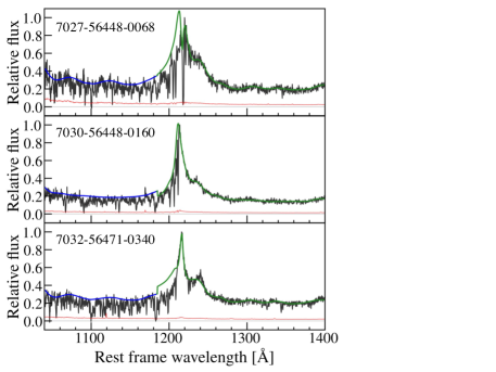
Our selection gives a total of $43$ background QSOs for the Hi tomography analysis. The distribution of the background QSOs is shown in Figure 2. The basic properties of the $43$ background QSOs are summarized in Table 6. Some example QSO spectra are shown in Figure 5.

Table 6: Background QSOs in the EGS field

ID	R.A.	Decl.	$z_{\rm spec}$	$g$
	(J2000)	(J2000)		(AB)
7339-56799-0270	14:14:08.64	+52:40:38.64	2.790	20.59
7339-56722-0800	14:14:18.24	+53:50:46.68	2.729	21.43
7339-56799-0734	14:14:20.64	+53:22:16.68	2.212	19.54
7339-56799-0730	14:14:35.52	+53:25:36.84	2.861	20.72
7339-56722-0297	14:14:39.12	+52:06:16.20	2.914	20.93
7339-56799-0728	14:14:44.16	+53:35:55.68	2.734	21.55
7339-56799-0277	14:15:08.64	+53:00:19.80	2.765	21.36
7340-56837-0794	14:15:41.04	+53:51:04.32	2.420	20.81
7027-56448-0068	14:15:51.36	+52:27:40.68	2.583	19.86
7028-56449-0809	14:16:45.12	+53:05:10.32	2.529	21.68
7339-56772-0218	14:16:47.28	+52:11:15.36	2.153	18.70
7340-56837-0833	14:17:22.32	+53:48:52.92	2.726	20.71
7339-56799-0831	14:17:50.40	+53:45:17.64	2.190	20.30
7339-56799-0854	14:18:07.68	+53:17:53.88	2.274	20.67
7339-56722-0876	14:18:17.52	+53:11:16.80	2.238	20.50
7339-56772-0893	14:18:43.20	+53:19:21.00	2.298	20.56
7340-56837-0117	14:19:12.48	+52:08:17.88	2.563	19.78
7339-56799-0087	14:19:52.80	+52:01:17.04	2.224	19.48
7339-56772-0924	14:20:10.56	+53:12:23.76	2.597	20.09
7027-56448-0994	14:20:33.12	+53:07:35.04	2.880	21.55
7340-56837-0923	14:20:41.28	+53:33:55.44	2.421	20.87
7339-56799-0074	14:21:13.20	+52:49:30.00	2.644	19.36
7339-56722-0074	14:21:18.00	+52:53:45.96	2.306	19.95
7339-56799-0069	14:21:38.64	+52:33:24.48	2.606	20.30
7339-56799-0068	14:21:41.28	+52:45:51.84	2.654	21.04
7339-56722-0062	14:21:55.20	+52:27:49.32	2.516	21.10
7339-56768-0038	14:22:39.60	+52:28:52.68	2.989	21.61
7339-56780-0074	14:22:42.48	+52:44:15.72	2.175	20.03
7340-56837-0978	14:23:06.00	+53:15:29.16	2.468	18.29
7029-56455-0100	14:23:17.28	+52:13:12.72	2.671	21.54
7032-56471-0340	14:23:37.20	+52:16:07.68	2.894	19.73
7339-56799-0992	14:24:11.04	+53:20:41.28	2.366	20.31
6710-56416-0442	14:24:11.52	+53:50:26.88	2.769	20.96
7339-56799-0014	14:24:18.24	+53:04:06.60	2.859	19.56
7339-56772-0972	14:24:19.20	+53:17:50.64	2.530	20.49
7032-56471-0306	14:24:27.84	+52:20:44.52	2.324	20.03
7029-56455-0955	14:24:33.12	+53:43:52.68	2.711	20.51
7030-56448-0160	14:24:50.88	+52:50:01.68	2.728	19.71
7030-56448-0130	14:24:55.68	+52:06:09.72	2.631	21.20
7031-56449-0356	14:24:58.56	+52:41:49.92	3.015	21.27
7031-56449-0334	14:25:06.24	+52:01:28.92	2.736	21.92
6710-56416-0446	14:25:09.12	+53:51:49.32	3.102	21.37
7032-56471-0729	14:25:10.80	+53:23:09.60	2.861	20.73

3 Hi TOMOGRAPHY TECHNIQUES AND MAPS

We carry out Hi tomography mapping that is a technique to reconstruct the 3D Hi LSSs based on Hi absorption features found in the sightlines to multiple background source spectra (e.g., Lee et al., 2018, 2014b, 2014a; Caucci et al., 2008; Pichon et al., 2001). This Section describes how we make Hi tomography maps from background source spectra (Section 3.1), and presents Hi tomography maps of the COSMOS and EGS fields (Section 3.2). Note that we make a new Hi tomography map only in the EGS field. This is because we use the public data of the Hi tomography map in the COSMOS field (Lee et al., 2018, Section 3.2.1).

3.1 Hi Tomography Techniques

Our Hi tomography analysis consists of the following two processes: 1) normalizing the background source spectra with estimated continua to create input spectra for Hi tomography (Section 3.1.1) and 2) reconstructing the Hi LSSs from the normalized spectra (Section 3.1.2).

3.1.1 Intrinsic Continua

To probe Hi absorption along the lines of sight to the background QSOs, we estimate the Ly $\alpha$ forest transmission in the $1041$ – $1185$ Å rest frame,

F(z)=f_{\rm obs}/f_{\rm int},

(1)

where $f_{\rm obs}$ is the observed continuum flux density and $f_{\rm int}$ is the intrinsic continuum flux density that is not affected by the Ly $\alpha$ forest absorption due to the IGM. We estimate $f_{\rm int}$ of our background QSOs, applying the continuum fitting technique of the mean-flux regulated/principal component analysis (MF-PCA; Lee et al. 2012) with the code developed by Lee et al. (2013; see also Lee et al. 2014b). In this technique, there are two steps. The first step is to fit spectral templates of QSOs to the observed spectra redward of Ly $\alpha$ to obtain initial estimates of the continuum spectra blueward of Ly $\alpha$ . In the same manner as Lee et al. (2014b), we use the spectral templates of QSOs constructed by Suzuki et al. (2005). The second step is to constrain the amplitude and slope of the blueward spectra that should match to previous measurements of the cosmic mean Ly $\alpha$ forest transmission, ${F_{\rm cos}(z)}$ . We adopt ${F_{\rm cos}(z)}$ estimated by Faucher-Giguère et al. (2008),

\displaystyle{F_{\rm cos}(z)}=\exp[-0.00185(1+z)^{3.92}].

(2)

With $F_{\rm cos}$ we estimate $f_{\rm int}$ (Figure 5), and use Equation (1) to obtain $F(z)$ . Note that the strong stellar and interstellar absorptions of Nii $\lambda 1084$ and Ciii $\lambda 1175$ associated with the QSO host galaxies in the Ly $\alpha$ forest wavelength range could bias the results. For conservative estimates, we do not use the spectra in the wavelength ranges of $\pm 5$ Å around these lines in our analyses. The uncertainties of $F(z)$ are calculated from the errors of the $f_{\rm obs}$ measurements and the $f_{\rm int}$ estimates based on the MF-PCA continuum fitting, the latter of which are evaluated by Lee et al. (2012) as a function of redshift and median S/N over the Ly $\alpha$ forest wavelength range (see Figure 8 of Lee et al. 2012). Specifically, we adopt MF-PCA continuum fitting errors of $7$ %, $6$ %, and $4$ % for spectra with median S/Ns over the Ly $\alpha$ forest wavelength ranges of $2$ – $4$ , $4$ – $10$ , and $>10$ , respectively.

Based on the estimated $F(z)$ and the cosmic mean Ly $\alpha$ forest transmission $F_{\rm cos}(z)$ , we calculate the Ly $\alpha$ forest fluctuation (hereafter referred to as Hi transmission overdensity) $\delta_{F}$ for our background QSOs,

\displaystyle\delta_{F}=\frac{F(z)}{F_{\rm cos}(z)}-1,

(3)

where negative values correspond to strong Hi absorptions. The errors of $\delta_{F}$ are calculated with the uncertainties of $F(z)$ . We confirm that the systematic effect of using different prescriptions of $F_{\rm cos}(z)$ obtained by Becker et al. (2013) and Inoue et al. (2014) is minor, only within $2$ %, which is not as large as the uncertainties of $F(z)$ .

Refer to caption — Figure 5: Example spectra of our background QSOs. The black (red) lines depict flux (error) per pixel. The grey lines show zero flux level. The green curves are the Suzuki et al. (2005) template overplotted at the source redshifts. The blue curves are the Suzuki et al. (2005) template representing the estimated continua.

3.1.2 Reconstruction Processes

Once we obtain the $\delta_{F}$ spectra of the background QSOs, we carry out Hi tomographic reconstruction to reveal the 3D distribution of the Hi gas. In the same manner as Lee et al. (2018, 2016, 2014b), we use the reconstruction code developed by Stark et al. (2015).⁴⁴4 https://github.com/caseywstark/dachshund The reconstruction code performs Wiener filtering for the estimated $\delta_{F}$ values along the sightlines of our background QSOs. The Wiener filtering is based on the following two calculations: the first is Gaussian smoothing with the scale of the mean transverse sightline separation $\langle d_{\perp}\rangle$ , which determines the spatial resolution of the tomography map; the second is input pixel weighting by the S/N to remove possible systematics caused by low S/N spectra.

Specifically, in the Wiener filtering, the reconstructed Hi transmission overdensity map $\delta_{F}^{\rm rec}$ is given by the following estimator (Stark et al., 2015; Lee et al., 2014a; Caucci et al., 2008; Pichon et al., 2001),

\delta_{F}^{\rm rec}=\mathbf{C}_{\mathrm{MD}}\cdot(\mathbf{C}_{\mathrm{DD}}+\mathbf{N})^{-1}\cdot\delta_{F}^{\rm obs},

(4)

where $\delta_{F}^{\rm obs}$ is the input Hi transmission overdensity datacube comprised of our background source spectra and coordinates. $\mathbf{C}_{\mathrm{MD}}$ , $\mathbf{C}_{\mathrm{DD}}$ , and $\mathbf{N}$ are the map-datacube, datacube-datacube, and noise covariances, respectively. The estimator, $\mathbf{C}_{\mathrm{MD}}\cdot(\mathbf{C}_{\mathrm{DD}}+\mathbf{N})^{-1}$ , is constructed so that it minimizes an expected error between the reconstructed $\delta_{F}^{\rm rec}$ and the actual Hi distribution (Stark et al., 2015, and references therein). The estimator also allows us to down-weight pixels in low S/N spectra. These covariances are assumed to be a Gaussian covariance between any two points $\mathbf{r_{1}}$ and $\mathbf{r_{2}}$ .

\mathbf{C}_{\mathrm{DD}}=\mathbf{C}_{\mathrm{MD}}=\mathbf{C(r_{1},r_{2})}

(5)

and

\mathbf{C(r_{1},r_{2})}=\sigma_{F}^{2}\exp\left[-\frac{(\Delta r_{\parallel})^{2}}{2L^{2}_{\parallel}}\right]\exp\left[-\frac{(\Delta r_{\perp})^{2}}{2L^{2}_{\perp}}\right],

(6)

where $\Delta r_{\parallel}$ and $\Delta r_{\perp}$ ( $L_{\parallel}$ and $L_{\perp}$ ) are the line-of-sight (LOS) and transverse distances between $\mathbf{r_{1}}$ and $\mathbf{r_{2}}$ (correlation lengths), respectively. We adopt $L_{\parallel}=L_{\perp}=\langle d_{\perp}\rangle$ as well as a normalization of $\sigma_{F}^{2}=0.05$ in the same manner as Lee et al. (2018, 2014b). More details about the reconstruction process is presented in Stark et al. (2015) and Lee et al. (2018).

3.2 Hi Tomography Maps

In the COSMOS field, we use the Hi tomography map of Lee et al. (2018) (Section 3.2.1), while in the EGS field we make the Hi tomography map with the $\delta_{F}$ spectra of our background QSOs (Section 3.2.2).

3.2.1 COSMOS

For the COSMOS field, we use the public data of the COSMOS Hi tomography map made by the CLAMATO survey (Lee et al., 2018) ⁵⁵5 https://clamato.lbl.gov/ . The COSMOS Hi tomography map is a 3D map of the IGM Hi absorption at $z=2.05$ – $2.55$ in a $0.157$ deg² area of the COSMOS field, having a $30\times\ 24\times\ 444\ h^{-3}{\rm cMpc}^{3}$ cosmic volume with a spatial resolution of $2.5$ $h^{-1}$ cMpc and a grid size of $0.5$ $h^{-1}$ cMpc. The Hi tomography map is reconstructed from the spectra of 240 background galaxies and QSOs at $z=2.2$ – $3.0$ . The sky distribution of these background sources is shown in Figure 2. Figures 7 and 7 present the COSMOS Hi tomography map and the $\delta_{F}$ pixel distribution, respectively. For error estimates in Section 4.1, we generate 1000 mock Hi tomography maps to which we give random perturbations following the Gaussian distribution with sigma defined by the data values of the error map, where the error map is estimated from the $1\sigma$ uncertainties of $\delta_{F}$ spectra of the background sources in the CLAMATO survey (Lee et al., 2018). The typical 1 $\sigma$ uncertainty of $\delta_{F}$ for a pixel in the Hi tomographic map is found to be about 0.1.

3.2.2 EGS

For the EGS field, we conduct large-scale Hi tomography mapping with our background QSOs (Figure 2). The mean transverse sightline separation is $\langle d_{\perp}\rangle$ $=20$ $h^{-1}$ cMpc which is about ten times larger than those of the background sources in the COSMOS field (Section 3.2.1). We aim to complement the COSMOS-field Hi tomography with the EGS-field Hi tomography that covers a large volume, albeit with coarse resolution. For our tomographic reconstruction, we choose a redshift range of $z=2.05$ – $2.55$ that is the same as the one of the COSMOS Hi tomography map (Lee et al., 2018, Section 3.2.1). This redshift range and the $6.0$ deg² sky area of the EGS field give an overall cosmic volume of $124\ \times 136\ \times 444\ h^{-3}{\rm cMpc}^{3}$ . We adopt a grid size of $1.0\ h^{-1}$ cMpc that over-samples the spatial resolution of $20$ $h^{-1}$ cMpc. Figures 9 and 9 present the EGS Hi tomography map and the $\delta_{F}$ pixel distribution, respectively. For error estimates, we create mock Ly $\alpha$ forest transmission data $F(z)$ for the $43$ background sightlines, adding Gaussian-distribution random noise based on the uncertainties of $F(z)$ that are obtained in Section 3.1.1. We then perform Hi tomography mapping with the mock data. Repeating this process to produce 100 mock Hi tomography maps, with the total limited by computing resources. The typical 1 $\sigma$ uncertainty of $\delta_{F}$ for a pixel in the Hi tomographic map is found to be about 0.1.

One might expect that the Hi-gas distribution in the EGS Hi tomography map could be affected by interpolation in the tomographic reconstruction process, due to the coarse distribution of sightlines. Recently, Ravoux et al. (2020) have simulated large-scale Hi tomography of eBOSS background QSOs whose sightline separation is $\simeq 15$ $h^{-1}$ cMpc, and demonstrated that the correlation of the reconstructed Hi-gas distribution and the underlying matter field is retained on large-scales. The correlation of Hi-gas and underlying matter is also investigated by Cai et al. (2016) and a strong correlation is suggested on $15-25$ $h^{-1}$ cMpc scales ⁶⁶6 It is noted that the Hi-gas distribution on a few Mpc scales can be affected by the strong ionizing radiation of the QSOs (Mukae et al., 2020; Momose et al., 2020). The simulation study of Ozbek et al. (2016) assessed the statistical properties of large-scale Hi tomography based on eBOSS background QSOs. They estimated the root-mean-square error for a $\delta_{F}$ pixel reconstructed with $\simeq 20$ $h^{-1}$ cMpc resolution is $\simeq 0.02$ which is smaller than the $\delta_{F}$ pixel error of the EGS Hi tomography map.

4 Results

In this section, we investigate the IGM Hi-gas distributions around $z\sim 2$ galaxies in our two Hi tomography maps.

4.1 Spatial Correlations Between Hi Gas and Galaxies

We present the results of spatial correlations between IGM Hi gas and galaxies in the COSMOS blank field. The results consist of two components: a 2D distribution map of $\delta_{F}$ as a function of distance and a radial profile of $\delta_{F}$ (hereafter Hi radial profiles) as a function of distance.

We measure $\delta_{F}$ around the 27 LAEs (Section 2.1) in our COSMOS Hi tomography map (Section 3.2.1) along the transverse $D$ and the line-of-sight (LOS) $Z$ directions. The comoving distances of $D$ and $Z$ are computed under the assumption of Hubble flow. We take the average of Hi tomography pixel arrays over a distance $\pm$ Z/2 $h^{-1}$ cMpc along the LOS direction at a fixed distance D $h^{-1}$ cMpc in the transverse direction from LAEs. Here we use Ly $\alpha$ redshifts for the redshifts of LAEs. We estimate $1\sigma$ errors of the averaged $\delta_{F}$ , calculating standard deviations of the measurements with the 1000 mock tomography maps (Section 3.2.1).

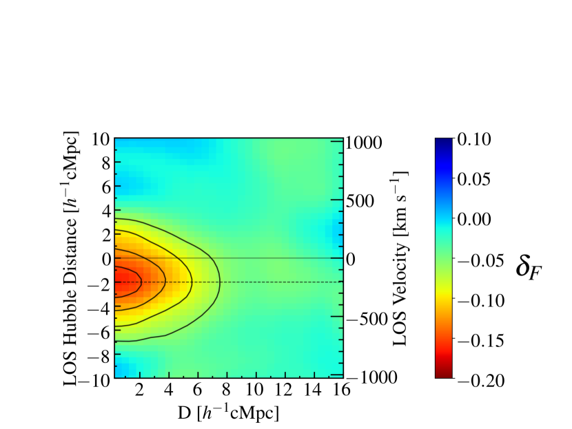
Figure 10 shows the 2D Hi distribution map of the COSMOS LAEs. In Figure 10, the LAEs are located at $(Z,D)=(0,0)$ $h^{-1}$ cMpc. There exist Hi absorption enhancements around LAEs at $-7\lesssim Z\lesssim 3$ $h^{-1}$ cMpc along the LOS direction and $D\lesssim 8$ $h^{-1}$ cMpc in the transverse direction from the LAEs. The Hi absorption enhancements have an anisotropic distribution whose Hi absorption peak has an offset toward the observer by $\sim 2\ h^{-1}{\rm cMpc}$ corresponding to the blueshift of $\sim 200$ km s^-1 from the LAE Ly $\alpha$ redshifts. This blueshift is consistent with the recent MUSE galaxy-background QSO pair study of Muzahid et al. (2019), and is explained by a well-known velocity offset of a Ly $\alpha$ redshift from a galaxy systemic redshift by $\sim 200$ km s^-1 for LAEs on average (Steidel et al. 2010; Hashimoto et al. 2013; Shibuya et al. 2014; Song et al. 2014; see Ouchi et al. 2020 in press and references therein) due to Ly $\alpha$ resonant scattering (e.g., Neufeld, 1990; Dijkstra et al., 2006). In other words, our 2D Hi distribution map reproduces the average $\sim 200$ km s^-1 offset of Ly $\alpha$ redshifts by the independent analysis that is different from previous studies requiring both galaxy Ly $\alpha$ and systemic redshift determinations from other spectral features.

Figure 10 also shows an elongated Hi-gas distribution whose absorption enhancements are stronger in the transverse direction than along the LOS direction from the Hi absorption peak. This elongation may originate from large-scale gas infall toward the galaxy halos as claimed in previous galaxy-background QSO pair studies (Turner et al., 2014; Bielby et al., 2017) and as predicted by numerical simulations (Turner et al., 2017; Kakiichi & Dijkstra, 2018). A detailed analysis with radiative transfer simulations for the elongated Hi-gas distribution will be presented in a forthcoming publication (Byrohl et al. in preparation).

We measure Hi radial profiles around the COSMOS LAEs (Section 2.1), spherically averaging radial profiles of $\delta_{F}$ taken from the COSMOS Hi tomography map (Section 3.2.1) as a function of 3D distance from the LAEs. This is the similar analysis of Hi-QSO performed in a previous study of Mukae et al. (2020). The 3D distances from the LAEs are defined as

\displaystyle R_{\rm 3D}\equiv\sqrt{D^{2}+d_{z}^{2}},

(7)

where $d_{z}$ is the Hubble flow comoving distance from the LAEs under the assumption that the Hi absorbers have zero peculiar velocities relative to the LAEs. To estimate uncertainties of the spherically averaged $\delta_{F}$ , we use the 1000 mock Hi tomography maps (Section 3.2.1). For each mock map, we compute Hi radial profiles averaged over our LAEs, to obtain $68$ % intervals as $1\sigma$ confidence intervals.

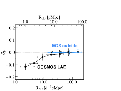
In Figure 11, the black circles present the average Hi radial profile of the COSMOS LAEs. The value of $\delta_{F}$ decreases (i.e., the Hi absorption increases) from the cosmic mean level $\delta_{F}$ $=0$ to $-0.1$ with decreasing $R_{\rm 3D}$ from $\sim 10$ $h^{-1}$ cMpc to $\sim 1$ $h^{-1}$ cMpc around the LAEs. In other words, our Hi radial profile shows strong Hi absorption exists around galaxies up to the 10 $h^{-1}$ cMpc scale. This trend is consistent with the one found for bright LAEs by Momose et al. (2020), whose Ly $\alpha$ luminosity limit for the bright LAEs is $L_{\rm Ly\alpha}\geq 10^{43}$ erg s^-1, comparable to the Ly $\alpha$ luminosity limit of the HETDEX LAEs (Section 2.1).

All of the results of the two components above indicate Hi absorption excesses around galaxies over Mpc scales (consistent with those of previous galaxy-background QSO pair studies of Turner et al. (2017), Bielby et al. (2017)), which confirm the impression of a spatial correlation between Hi and galaxies seen in Figure 12. Note that these results of the spatial correlations are free from influences of bright type-I QSOs, because no eBOSS QSOs at $z=2.05$ – $2.55$ are found in the cosmic volume of the COSMOS Hi tomography map (Section 2.2.1).

4.2 Hi–Gas Distribution Around an Extreme QSO Overdensity

We investigate the IGM Hi-gas distribution around QSOs and galaxies in an extreme QSO overdensity.

First, we search for QSO overdensities in the large $6.0$ -deg² area of the EGS field that is sufficient to find rare systems of QSO overdensities (e.g., Cai et al., 2017; Hennawi et al., 2015). We use the 78 foreground QSOs (Section 2.2.1), and estimate QSO overdensities within a sphere of radius 20 $h^{-1}$ cMpc at $z=2.3$ . This radius is larger than the one applied for galaxy overdensity measurements (Chiang et al., 2013, 2014), because the number density of QSOs is about two orders of magnitude smaller than that of galaxies at $z\sim 2$ . The QSO overdensity is defined as

\delta_{\rm QSO}\equiv\frac{n_{\rm QSO}}{\overline{n}_{\rm QSO}}-1,

(8)

where $n_{\rm QSO}$ ( $\overline{n}_{\rm QSO}$ ) is the number density (mean number density) of the QSOs in a sphere. The mean number density is derived in the cosmic volume of the Hi tomography map. The expected number of QSOs in the sphere is about $0.35$ comparable to that estimated from QSO luminosity functions (e.g., Palanque-Delabrouille et al., 2013) integrated to the detection limit of the eBOSS QSOs ( $g\simeq 22$ mag). We calculate $\delta_{\rm QSO}$ at pixel positions of the EGS Hi tomography map, and make a $\delta_{\rm QSO}$ map whose volume coverage is similar to that of the Hi tomography map. Searching for the largest QSO overdensity in the $\delta_{\rm QSO}$ map, we find an extremely high overdensity at $z=2$ , dubbed EGS-QO1, whose QSO overdensity is $\delta_{\rm QSO}$ $=16.2\pm 7.0$ . The top panel of Figure 13 shows a projection of a $40\ h^{-1}$ cMpc-width slice of our $\delta_{\rm QSO}$ map with EGS-QO1. The overdensity of EGS-QO1 is clearly distinguished.

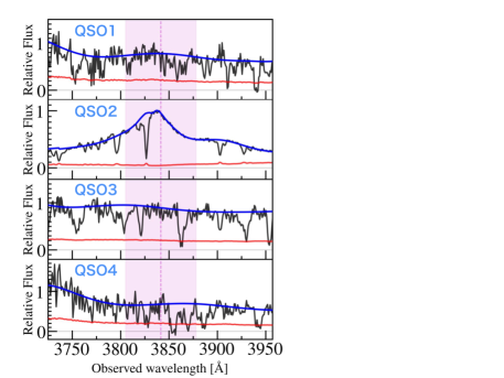
Next, we inspect the Hi environment of EGS-QO1 with the Hi tomography map. The bottom panel of Figure 13 shows the projected Hi tomography map of the same slice as presented in the top panel of Figure 13. Comparing the top and bottom panels of Figure 13, we find that EGS-QO1 resides in an Hi underdensity volume with a size of $\sim 40\ \times 70\ \times 40\ h^{-3}{\rm cMpc}^{3}$ at $z=2.13$ – $2.19$ (centered at $\left<z\right>=2.16$ ). Red histogram in Figure 9 depicts the $\delta_{F}$ pixel distribution of EGS-QO1. The Hi absorption values in EGS-QO1 ranges $\delta_{F}$ $\simeq 0.1-0.4$ , indicating that the EGS-QO1 resides in an Hi underdensity volume. Note that the typical 1 $\sigma$ uncertainty of $\delta_{F}$ for a pixel in the Hi tomographic map is $0.1$ (Section 3.2.2). Although no background QSOs probe Hi absorption at the exact sky center of the Hi underdensity volume, spectra of several of the QSOs distributed over this volume show evidence of the Hi underdensity (Figure 14). The Hi underdensity associated with the QSO overdensity suggests that the QSOs forming the EGS-QO1 overdensity would make a large ionized bubble, where the Hi gas is widely photoionized by the strong ionizing radiation of the QSOs.

The ionized bubble may be created by overlap of proximity zones of the QSOs, each of which should have a typical size of $\sim 10-15\ h^{-1}$ cMpc in diameter at $z\sim 2$ (e.g., D’Odorico et al., 2008; Mukae et al., 2020; Jalan et al., 2019). If the ionized bubble length of $\sim 40$ $h^{-1}$ cMpc is made by three QSOs roughly distributed along the redshift direction in EGS-QO1, each QSO would form a proximity zone with $40/3\simeq 13$ $h^{-1}$ cMpc in diameter, which is comparable to typical sizes in the literature. When the proximity zone size is simply divided by the speed of light, we obtain QSO lifetimes of $t_{\rm QSO}=10^{7.3}$ years consistent with typical values of $t_{\rm QSO}=10^{7-9}$ years that are constrained by clustering measurements (e.g., Adelberger & Steidel, 2005; White et al., 2012; Conroy & White, 2013).

Note that the Hi absorption is made by the ionized IGM with Hi fraction as low as $\sim 0.6\times 10^{-6}$ ⁷⁷7The Hi fraction is obtained with a ratio of the EGS-QO1 value to the cosmic value at $z=2$ (McQuinn, 2016). The ratio is simply estimated from a ratio of column densities that are converted from optical depth of $\delta_{F}$ $\simeq 0.2$ (the peak value of the $\delta_{F}$ fraction in Figure 9) and $\delta_{F}$ $=0.0$ (the cosmic mean value) under the assumption of optically-thin Ly $\alpha$ forest clouds (Draine, 2011; Mo et al., 2010).. Even outside of the ionized bubble, the IGM is highly ionized with the cosmic average Hi fraction of $\sim 2.0\times 10^{-6}$ at $z=2$ (McQuinn, 2016). The ionized bubble defined here is the cosmic volume with small Hi fraction that is probably caused by the strong QSO radiation.

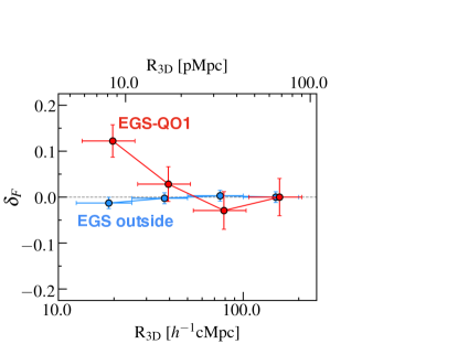
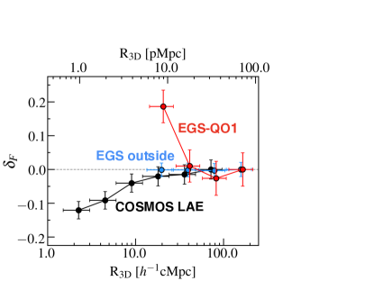
We then measure the Hi radial profile averaged over the six QSOs forming the EGS-QO1 overdensity. Figure 15 represents the average Hi radial profile around the six QSOs. The $\delta_{F}$ values increase (i.e., Hi absorption weakens) from the cosmic mean level ( $\delta_{F}$ $=0$ ) to $\delta_{F}$ $=0.1$ with decreasing $R_{\rm 3D}$ from $\sim 100$ $h^{-1}$ cMpc to $\sim 10$ $h^{-1}$ cMpc around the QSOs. This Hi radial profile suggests strongly-suppressed Hi absorption around the QSOs in the extreme QSO overdensity. It is a clear contrast with the results of the blank fields; the Hi radial profile of the rest of 72 QSOs that reside outside of the EGS-QO1 (here after referred to as EGS outside; Figure 15) and the Hi radial profile of galaxies in the COSMOS field (Figure 11).

Here we need to examine whether this contrast is made by the choices of the Hi radial profile measurement centers (QSOs vs. galaxies) or the environment (QSO overdensity vs. blank field). In the cosmic volume of the EGS Hi tomography map, we find 26 LAEs, four of which reside in the EGS-QO1 QSO overdensity at $z=2.13$ – $2.19$ . These four LAEs, dubbed LAE1-4 are shown with black circles and white labels in Figure 13. In EGS-QO1, the density of LAEs is high, and there is a moderate LAE overdensity of $\sim 1$ in a radius of 20 $h^{-1}$ cMpc. Figure 16 presents the HETDEX spectra and CFHT/HST images of LAE1-4. We calculate Hi radial profiles around LAE1-4 in the EGS-QO1 QSO overdensity in the same manner as Section 4.1, and show the average Hi radial profile in Figure 17. We find that this Hi radial profile around the LAEs (Figure 17) is similar to that of the QSOs in EGS-QO1 (Figure 15) and clearly different from the one around LAEs in the blank field (Figure 11). We also measure the Hi radial profiles around the rest of 22 LAEs that reside outside of EGS-QO1 (i.e. EGS outside; Figure 11), and find that the Hi radial profile is consistent with the one in the blank field on the scale down to $\sim 20$ $h^{-1}$ cMpc the resolution limit of the EGS Hi tomography map. In other words, the Hi absorption is significantly weakened around galaxies in the QSO overdensity EGS-QO1, in contrast with the strong Hi absorption around galaxies in the blank field (Section 4.1). The weak Hi absorption around galaxies found in EGS-QO1 is probably caused by the environment of the QSO overdensity that produces the ionized bubble.

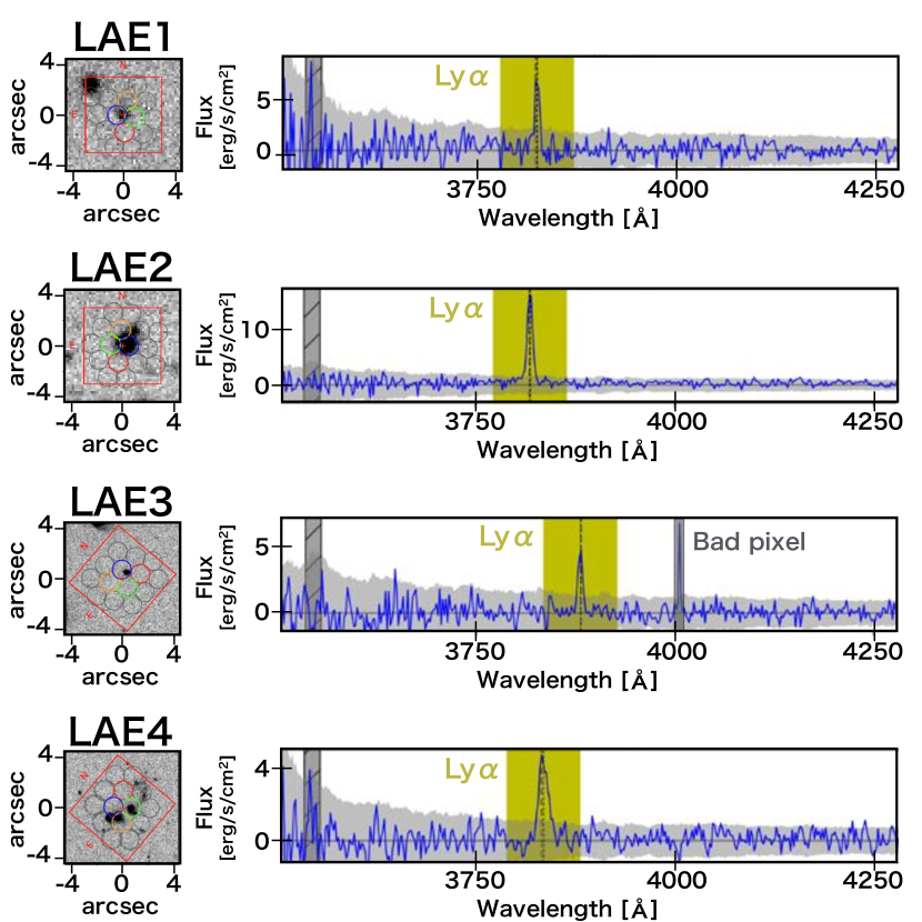
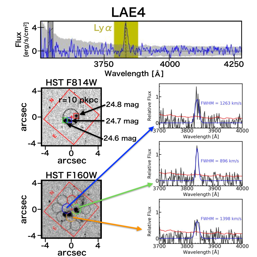
We find that one of the four LAEs, LAE4, shows triple-continuum components over the scale of a 10 pkpc-radius circle on the HST F814W/F160W images of the EGS, indicative of a triple merging system (middle/bottom panels of Figure 18). LAE4 is located at (R.A., Decl.) $=$ (14:19:13.02, +52:49:11.2) near the center of the ionized bubble of EGS-QO1 (bottom panel of Figure 13). The average Ly $\alpha$ redshift of LAE4 over the HETDEX fibers is $z_{\rm Ly\alpha}=2.156$ , and the total Ly $\alpha$ luminosity over the fibers is $L_{\rm Ly\alpha}^{*}=10^{43.06}$ erg s^-1. The top panel of Figure 18 presents the spectrum of LAE4, summed over the fibers, which is the same as the one in Figure 16. The spectrum of LAE4 has a broad Ly $\alpha$ emission line whose FWHM is $\sim 1100$ km s^-1 (about 3 times broader than the instrumental resolution), possibly suggesting a type-I AGN (e.g. Kakuma et al. in preparation)⁸⁸8Other AGN features of high-ionization emission lines, Civ $\lambda 1549$ Å and Heii $\lambda 1640$ Å, are not detected in the LAE4 spectrum shown in Figure 16. This is probably because the LAE4 is optically faint ( $\sim$ 25 mag) and its metal lines are too faint to be identified.. The bottom panel of Figure 18 presents the positions and the sky coverage of the fibers used for the measurements of the LAE4 Ly $\alpha$ redshift and total luminosity, and indicates three fibers cover the triple-continuum components with the blue, green, and yellow circles. The spectra of these three fibers are shown on the right-hand side in Figure 18. All of the three fiber spectra of the blue, green, and yellow circles have Ly $\alpha$ emission lines at $z_{\rm Ly\alpha}=2.16$ , suggesting that the three objects probably reside at the same redshift. Moreover, these three fiber spectra have broad Ly $\alpha$ emission lines with an FWHM of $\sim 1000$ km s^-1. Although each of these fibers does not separately cover one of the triple-continuum components whose blending due to the HET image quality and large fiber diameter may produce apparent broad lines, these broad Ly $\alpha$ emission lines found in the different positions over the triple-continuum components imply that the LAE4 system could be a merging type-I AGN doublet or triplet.

5 Discussion

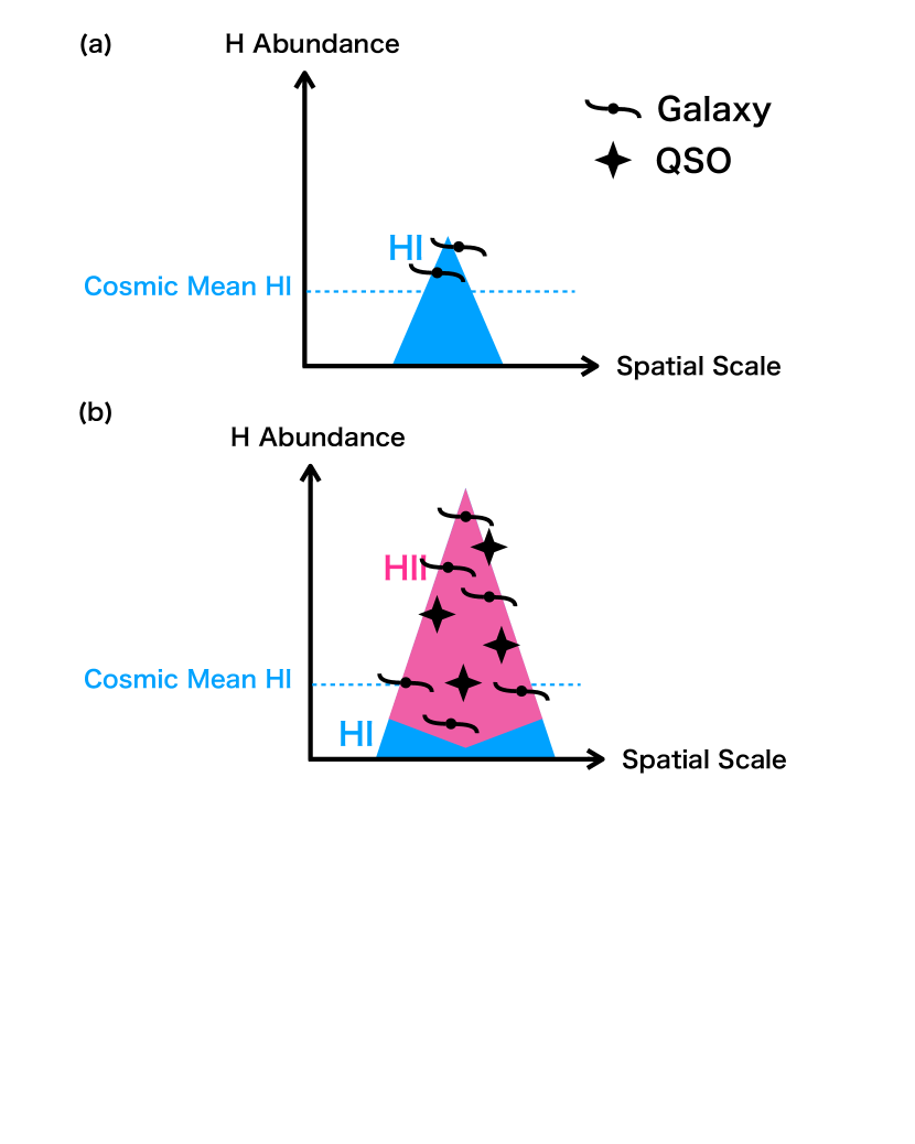
In Section 4.1, we have investigated spatial correlations between IGM Hi-gas and galaxies in the COSMOS field, the blank field with no QSO overdensities. We have found that strong Hi absorption exists around galaxies up to the 10 $h^{-1}$ cMpc scale. The result suggests a picture where a galaxy resides in an Hi-gas overdensity in a blank field as illustrated in Figure 19 (a).

In Section 4.2, we have studied spatial correlations between IGM Hi-gas and galaxies in the EGS field, where the extreme QSO overdensity EGS-QO1 of six QSOs is found. There is also a galaxy overdensity in EGS-QO1, traced by LAEs. In the Hi tomography map of the EGS field, EGS-QO1 resides in an ionized bubble with a size of $\sim 40$ $h^{-1}$ cMpc at $\left<z\right>=2.16$ . In fact, the galaxies and the QSOs in and around EGS-QO1 statistically show weak Hi absorption. Because Hi absorption is weakened in the EGS-QO1 QSO overdensity unlike in the blank field, we infer that the QSOs of EGS-QO1 probably produce an ionized bubble as a result of the overlap of multiple proximity zones of the QSOs, where a galaxy overdensity with a large Hi-gas overdensity originally existed. This physical picture is illustrated in Figure 19 (b).

The relationship between the physical pictures of Figure 19 (a) and (b) may be explained by evolution of photoionization of Hi gaseous LSSs. A matter overdensity in LSSs produces the overdensities of Hi gas and galaxies (Cai et al., 2017, 2016). Once QSO activity is triggered in the galaxies, Hi gas in the overdensity is photoionized by photons from the QSOs (Mukae et al., 2020; Momose et al., 2020). ⁹⁹9 A timeline of this evolutional process is not clear. It may be possible for a large Hi-gas overdensity (as in Figure 19 b) to form first almost completely, and that subsequently QSOs appear to ionize the Hi gas. However, it is more likely that QSOs gradually ionize the Hi gas at the assembly stage of the large Hi-gas overdensity. This makes a cosmic volume of weak Hi absorption corresponding to the ionized bubble. Note that again the ionized bubble has a low Hi fraction that can be even smaller than that of the cosmic average Hi fraction at $z\sim 2$ in the universe after cosmic reionization (Section 4.2).

6 Summary

We have investigated IGM Hi gas distributions around $z\sim 2$ galaxies in two galaxy environments: a blank field (COSMOS) and an extreme QSO overdensity field (EGS). Combining the large survey datasets of galaxies and QSOs that are provided by HETDEX LAEs and SDSS-IV/eBOSS QSOs, respectively, we construct the samples of foreground galaxies and QSOs at $z\sim 2$ as well as the sample of background QSOs at $z>2$ . In the sample of foreground QSOs, we have identified the extreme QSO overdensity, EGS-QO1, consisting of six QSOs in a radius of 20 $h^{-1}$ cMpc.

For the COSMOS field, we use the Hi tomography map of Lee et al. (2018), while for the EGS field we reconstruct 3D Hi LSSs by performing Hi tomography based on Hi absorption found in the spectra of background QSOs. These COSMOS and EGS Hi tomography maps have cosmic volumes of ( $30\times 24\times 444$ , $124\times 136\times 444$ ) $\ h^{-3}$ cMpc³, respectively, at $z=2.3$ . We have investigated spatial correlations between the Hi absorption and the galaxies in the two Hi tomography maps. Our findings are listed below.

1.

In the blank field of COSMOS that has no eBOSS QSOs within the volume of the tomography map, the spherically averaged Hi radial profiles indicate that Hi absorption around galaxies is stronger than those of the cosmic average at a distance from these galaxies up to $10$ $h^{-1}$ cMpc. Stronger Hi absorption is found closer to the galaxies. The same trends are also found in the averaged 2D Hi absorption map (transverse vs. LOS distances). These results suggest that the IGM Hi gas and galaxies (LAEs) are spatially correlated, and that more Hi gas exists around such galaxies.
2.

In the averaged 2D Hi absorption map shown in Figure 10, there is an anisotropy in the transverse and LOS directions. On average, the Hi absorption peak is blueshifted by $\sim 200$ km s^-1 from the galaxy Ly $\alpha$ redshift. This result independently reproduces the known average velocity offset between the Ly $\alpha$ emission redshift and the galaxy systemic redshift, using a completely independent tracer.
3.

The extreme QSO overdensity of EGS-QO1 resides in an Hi underdensity volume with a size of $\sim 40\ \times 70\ \times 40\ h^{-3}{\rm cMpc}^{3}$ at $z=2.13$ – $2.19$ (centered at $\left<z\right>=2.16$ ). In this volume, the spherically-averaged Hi radial profiles show that Hi absorption around galaxies (and QSOs) is weaker than that of the cosmic average, and that the weaker Hi absorption exists closer to the galaxies (and the QSOs). These results contrast with those of the blank fields of COSMOS and EGS outside of EGS-QO1. Interestingly, in the EGS Hi tomography map, we identify an ionized bubble with a size of $\sim 40$ $h^{-1}$ cMpc at $\left<z\right>=2.16$ in the volume of the EGS-QO1. The ionized bubble may form due to intense ionizing photon radiation as a result of the overlap of multiple proximity zones of the QSOs.
4.

As noted above, we find possible opposite trends of the Hi-galaxy spatial correlation in the two fields, the blank field and the extreme QSO overdensity field. A schematic illustration of our interpretation is shown in Figure 19. Although matter overdensities produce galaxies and galaxy+QSO overdensities, QSOs, if present, ionize the hydrogen gas around galaxies in the overdensity. In an extreme QSO overdensity, the negative correlation of the Hi-galaxy spatial distribution is probably created by ionizing radiation of the QSOs. If our interpretation (Figure 19) is correct, the two different trends of Hi-galaxy spatial correlation may be explained by evolution of photoionization in Hi gaseous LSSs. In other words, once QSO activity emerges in galaxies residing in an Hi gas overdensity, the Hi gas around the galaxies is photoionized by the ionizing photons of the QSOs.

The evolutionary picture is based on one QSO overdensity (EGS-QO1). More QSO overdensities should be investigated to statistically test the picture as well as the morphology of giant ionized bubbles, because QSOs are actually complicated systems whose proximity zones relate to physical quantities such as the number of ionizing photons, the opening angle for ionizing photon escape, the lifetime, and the duty cycle (e.g., Bosman et al., 2020; Adelberger, 2004). Further investigation will be made with forthcoming data from the HETDEX survey. Future data releases are expected to have improved spectral traces, sky subtraction, cosmic-ray removal, and flux calibration (Gebhardt et al. 2020, in preparation). The HETDEX survey will ultimately provide $10^{6}$ galaxies with spectroscopic redshifts at $z=1.9$ – $3.5$ in a $9$ Gpc³ volume. The HETDEX survey will statistically reveal the galaxy - IGM Hi relation as a function of QSO overdensities in the large HETDEX Spring Field (300 deg²; Hill & HETDEX Consortium 2016). Such statistical studies of LSS photoionization will shed light not only on the suppression of the formation of low-mass galaxies due to enhanced UVB radiation, but also the ionization processes of the intra-cluster media of galaxy clusters.

We thank the anonymous referee for constructive comments and suggestions that definitely improved the clarity of the paper. We are grateful to Koki Kakiichi, Siddhartha Gurung-Lopez, and Chris Sneden for their useful discussions and comments. HETDEX is led by the University of Texas at Austin McDonald Observatory and Department of Astronomy with participation from the Ludwig-Maximilians- Universität München, Max-Planck-Institut für Extraterrestrische-Physik (MPE), Leibniz-Institut für Astrophysik Potsdam (AIP), Texas A&M University, Pennsylvania State University, Institut für Astrophysik Göttingen, The University of Oxford, Max-Planck-Institut für Astrophysik (MPA), The University of Tokyo and Missouri University of Science and Technology. In addition to Institutional support, HETDEX is funded by the National Science Foundation (grant AST-0926815), the State of Texas, the US Air Force (AFRL FA9451-04-2- 0355), and generous support from private individuals and foundations. The observations were obtained with the Hobby-Eberly Telescope (HET), which is a joint project of the University of Texas at Austin, the Pennsylvania State University, Ludwig-Maximilians-Universität München, and Georg-August-Universität G0̈ttingen. The HET is named in honor of its principal benefactors, William P. Hobby and Robert E. Eberly. VIRUS is a joint project of the University of Texas at Austin, Leibniz-Institut für Astrophysik Potsdam (AIP), Texas A&M University, Max-Planck-Institut für Extraterrestrische-Physik (MPE), Ludwig-Maximilians- Universität München, The University of Oxford, Pennsylvania State University, Institut für Astrophysik Göttingen,, Max-Planck-Institut für Astrophysik (MPA) The Texas Advanced Computing Center (TACC) at The University of Texas at Austin provided high performance computing, visualization, and storage resources that contributed to the research results reported within this paper. The Institute for Gravitation and the Cosmos is supported by the Eberly College of Science and the Office of the Senior Vice President for Research at The Pennsylvania State University. This paper is supported by World Premier International Research Center Initiative (WPI Initiative), MEXT, Japan, and KAKENHI (15H02064, 17H01110, and 17H01114) Grant-in-Aid for Scientific Research (A) through Japan Society for the Promotion of Science. S.M acknowledges support from the JSPS through the JSPS Research Fellowship for Young Scientists. Funding for the Sloan Digital Sky Survey IV has been provided by the Alfred P. Sloan Foundation, the U.S. Department of Energy Office of Science, and the Participating Institutions. SDSS-IV acknowledges support and resources from the Center for High-Performance Computing at the University of Utah. The SDSS web site is www.sdss.org. SDSS-IV is managed by the Astrophysical Research Consortium for the Participating Institutions of the SDSS Collaboration including the Brazilian Participation Group, the Carnegie Institution for Science, Carnegie Mellon University, the Chilean Participation Group, the French Participation Group, Harvard-Smithsonian Center for Astrophysics, Instituto de Astrofísica de Canarias, The Johns Hopkins University, Kavli Institute for the Physics and Mathematics of the Universe (IPMU) / University of Tokyo, the Korean Participation Group, Lawrence Berkeley National Laboratory, Leibniz Institut für Astrophysik Potsdam (AIP), Max-Planck-Institut für Astronomie (MPIA Heidelberg), Max-Planck-Institut für Astrophysik (MPA Garching), Max-Planck-Institut für Extraterrestrische Physik (MPE), National Astronomical Observatories of China, New Mexico State University, New York University, University of Notre Dame, Observatário Nacional / MCTI, The Ohio State University, Pennsylvania State University, Shanghai Astronomical Observatory, United Kingdom Participation Group, Universidad Nacional Autónoma de México, University of Arizona, University of Colorado Boulder, University of Oxford, University of Portsmouth, University of Utah, University of Virginia, University of Washington, University of Wisconsin, Vanderbilt University, and Yale University.

References

Adelberger (2004) Adelberger, K. L. 2004, ApJ, 612, 706
Adelberger et al. (2005) Adelberger, K. L., Shapley, A. E., Steidel, C. C., et al. 2005, ApJ, 629, 636
Adelberger & Steidel (2005) Adelberger, K. L., & Steidel, C. C. 2005, ApJ, 630, 50
Becker et al. (2013) Becker, G. D., Hewett, P. C., Worseck, G., & Prochaska, J. X. 2013, MNRAS, 430, 2067
Bielby et al. (2017) Bielby, R. M., Shanks, T., Crighton, N. H. M., et al. 2017, MNRAS, 471, 2174
Bosman et al. (2020) Bosman, S. E. I., Kakiichi, K., Meyer, R. A., et al. 2020, ApJ, 896, 49
Cai et al. (2016) Cai, Z., Fan, X., Peirani, S., et al. 2016, ApJ, 833, 135
Cai et al. (2017) Cai, Z., Fan, X., Bian, F., et al. 2017, ApJ, 839, 131
Caucci et al. (2008) Caucci, S., Colombi, S., Pichon, C., et al. 2008, MNRAS, 386, 211
Chiang et al. (2013) Chiang, Y.-K., Overzier, R., & Gebhardt, K. 2013, ApJ, 779, 127
Chiang et al. (2014) —. 2014, ApJ, 782, L3
Conroy & White (2013) Conroy, C., & White, M. 2013, ApJ, 762, 70
Davis et al. (2007) Davis, M., Guhathakurta, P., Konidaris, N. P., et al. 2007, ApJ, 660, L1
Dawson et al. (2016) Dawson, K. S., Kneib, J.-P., Percival, W. J., et al. 2016, AJ, 151, 44
Dekel et al. (2009) Dekel, A., Birnboim, Y., Engel, G., et al. 2009, Nature, 457, 451
Dijkstra et al. (2006) Dijkstra, M., Haiman, Z., & Spaans, M. 2006, ApJ, 649, 14
D’Odorico et al. (2008) D’Odorico, V., Bruscoli, M., Saitta, F., et al. 2008, MNRAS, 389, 1727
Draine (2011) Draine, B. T. 2011, Physics of the Interstellar and Intergalactic Medium
Evans et al. (2012) Evans, C. J., Barbuy, B., Bonifacio, P., et al. 2012, in Society of Photo-Optical Instrumentation Engineers (SPIE) Conference Series, Vol. 8446, Ground-based and Airborne Instrumentation for Astronomy IV, 84467K
Faucher-Giguère et al. (2008) Faucher-Giguère, C.-A., Prochaska, J. X., Lidz, A., Hernquist, L., & Zaldarriaga, M. 2008, ApJ, 681, 831
Fox & Davè (2017) Fox, A., & Davè, R. 2017, Gas Accretion onto Galaxies, Vol. 430 (Basel: Springer International Publishing AG), doi:10.1007/978-3-319-52512-9
Hashimoto et al. (2013) Hashimoto, T., Ouchi, M., Shimasaku, K., et al. 2013, ApJ, 765, 70
Hennawi et al. (2015) Hennawi, J. F., Prochaska, J. X., Cantalupo, S., & Arrigoni-Battaia, F. 2015, Science, 348, 779
Hill (2014) Hill, G. J. 2014, Advanced Optical Technologies, 3, 265
Hill & HETDEX Consortium (2016) Hill, G. J., & HETDEX Consortium. 2016, in Astronomical Society of the Pacific Conference Series, Vol. 507, Multi-Object Spectroscopy in the Next Decade: Big Questions, Large Surveys, and Wide Fields, ed. I. Skillen, M. Barcells, & S. Trager, 393
Hill et al. (2008) Hill, G. J., Gebhardt, K., Komatsu, E., et al. 2008, in Astronomical Society of the Pacific Conference Series, Vol. 399, Panoramic Views of Galaxy Formation and Evolution, ed. T. Kodama, T. Yamada, & K. Aoki, 115
Hill et al. (2018a) Hill, G. J., Kelz, A., Lee, H., et al. 2018a, in Society of Photo-Optical Instrumentation Engineers (SPIE) Conference Series, Vol. 10702, Proc. SPIE, 107021K
Hill et al. (2018b) Hill, G. J., Drory, N., Good, J. M., et al. 2018b, in Society of Photo-Optical Instrumentation Engineers (SPIE) Conference Series, Vol. 10700, Ground-based and Airborne Telescopes VII, 107000P
Hinshaw et al. (2013) Hinshaw, G., Larson, D., Komatsu, E., et al. 2013, ApJS, 208, 19
Inoue et al. (2014) Inoue, A. K., Shimizu, I., Iwata, I., & Tanaka, M. 2014, MNRAS, 442, 1805
Jalan et al. (2019) Jalan, P., Chand, H., & Srianand, R. 2019, ApJ, 884, 151
Kakiichi & Dijkstra (2018) Kakiichi, K., & Dijkstra, M. 2018, MNRAS, 480, 5140
Kashikawa et al. (2007) Kashikawa, N., Kitayama, T., Doi, M., et al. 2007, ApJ, 663, 765
Kelz et al. (2014) Kelz, A., Jahn, T., Haynes, D., et al. 2014, Society of Photo-Optical Instrumentation Engineers (SPIE) Conference Series, Vol. 9147, VIRUS: assembly, testing and performance of 33,000 fibres for HETDEX, 914775
Kereš et al. (2005) Kereš, D., Katz, N., Weinberg, D. H., & Davé, R. 2005, MNRAS, 363, 2
Kikuta et al. (2017) Kikuta, S., Imanishi, M., Matsuoka, Y., et al. 2017, ApJ, 841, 128
Kikuta et al. (2019) Kikuta, S., Matsuda, Y., Cen, R., et al. 2019, PASJ, 71, L2
Lee et al. (2014a) Lee, K.-G., Hennawi, J. F., White, M., Croft, R. A. C., & Ozbek, M. 2014a, ApJ, 788, 49
Lee et al. (2012) Lee, K.-G., Suzuki, N., & Spergel, D. N. 2012, AJ, 143, 51
Lee et al. (2013) Lee, K.-G., Bailey, S., Bartsch, L. E., et al. 2013, AJ, 145, 69
Lee et al. (2014b) Lee, K.-G., Hennawi, J. F., Stark, C., et al. 2014b, ApJ, 795, L12
Lee et al. (2016) Lee, K.-G., Hennawi, J. F., White, M., et al. 2016, ApJ, 817, 160
Lee et al. (2018) Lee, K.-G., Krolewski, A., White, M., et al. 2018, ApJS, 237, 31
Leung et al. (2017) Leung, A. S., Acquaviva, V., Gawiser, E., et al. 2017, ApJ, 843, 130
Liang et al. (2020) Liang, Y., Kashikawa, N., Cai, Z., et al. 2020, arXiv e-prints, arXiv:2008.01733
McQuinn (2016) McQuinn, M. 2016, ARA&A, 54, 313
Meiksin (2009) Meiksin, A. A. 2009, Reviews of Modern Physics, 81, 1405
Mo et al. (2010) Mo, H., van den Bosch, F. C., & White, S. 2010, Galaxy Formation and Evolution (Cambridge: Cambridge Univ. Press)
Momose et al. (2020) Momose, R., Shimasaku, K., Kashikawa, N., et al. 2020, arXiv e-prints, arXiv:2002.07335
Mukae et al. (2017) Mukae, S., Ouchi, M., Kakiichi, K., et al. 2017, ApJ, 835, 281
Mukae et al. (2020) Mukae, S., Ouchi, M., Cai, Z., et al. 2020, ApJ, 896, 45
Muzahid et al. (2019) Muzahid, S., Schaye, J., Marino, R. A., et al. 2019, arXiv e-prints, arXiv:1910.03593
Nagamine et al. (2020) Nagamine, K., Shimizu, I., Fujita, K., et al. 2020, arXiv e-prints, arXiv:2007.14253
Neufeld (1990) Neufeld, D. A. 1990, ApJ, 350, 216
Newman et al. (2020) Newman, A. B., Rudie, G. C., Blanc, G. A., et al. 2020, ApJ, 891, 147
Noterdaeme et al. (2012) Noterdaeme, P., Petitjean, P., Carithers, W. C., et al. 2012, A&A, 547, L1
Oke & Gunn (1983) Oke, J. B., & Gunn, J. E. 1983, ApJ, 266, 713
Ozbek et al. (2016) Ozbek, M., Croft, R. A. C., & Khandai, N. 2016, MNRAS, 456, 3610
Palanque-Delabrouille et al. (2013) Palanque-Delabrouille, N., Magneville, C., Yèche, C., et al. 2013, A&A, 551, A29
Pâris et al. (2017) Pâris, I., Petitjean, P., Ross, N. P., et al. 2017, A&A, 597, A79
Pâris et al. (2018) Pâris, I., Petitjean, P., Aubourg, É., et al. 2018, A&A, 613, A51
Pichon et al. (2001) Pichon, C., Vergely, J. L., Rollinde, E., Colombi, S., & Petitjean, P. 2001, MNRAS, 326, 597
Ramsey et al. (1994) Ramsey, L. W., Sebring, T. A., & Sneden, C. A. 1994, Society of Photo-Optical Instrumentation Engineers (SPIE) Conference Series, Vol. 2199, Spectroscopic survey telescope project, ed. L. M. Stepp, 31–40
Ravoux et al. (2020) Ravoux, C., Armengaud, E., Walther, M., et al. 2020, arXiv e-prints, arXiv:2004.01448
Shibuya et al. (2014) Shibuya, T., Ouchi, M., Nakajima, K., et al. 2014, ApJ, 788, 74
Somerville & Davé (2015) Somerville, R. S., & Davé, R. 2015, ARA&A, 53, 51
Song et al. (2014) Song, M., Finkelstein, S. L., Gebhardt, K., et al. 2014, ApJ, 791, 3
Stark et al. (2015) Stark, C. W., White, M., Lee, K.-G., & Hennawi, J. F. 2015, MNRAS, 453, 311
Steidel et al. (2009) Steidel, C., Martin, C., Prochaska, J. X., et al. 2009, in astro2010: The Astronomy and Astrophysics Decadal Survey, Vol. 2010, 286
Steidel et al. (2010) Steidel, C. C., Erb, D. K., Shapley, A. E., et al. 2010, ApJ, 717, 289
Susa & Umemura (2000) Susa, H., & Umemura, M. 2000, ApJ, 537, 578
Susa & Umemura (2004) —. 2004, ApJ, 600, 1
Suzuki et al. (2005) Suzuki, N., Tytler, D., Kirkman, D., O’Meara, J. M., & Lubin, D. 2005, ApJ, 618, 592
Turner et al. (2017) Turner, M. L., Schaye, J., Crain, R. A., et al. 2017, MNRAS, 471, 690
Turner et al. (2014) Turner, M. L., Schaye, J., Steidel, C. C., Rudie, G. C., & Strom, A. L. 2014, MNRAS, 445, 794
Umehata et al. (2019) Umehata, H., Fumagalli, M., Smail, I., et al. 2019, Science, 366, 97
van de Voort (2017) van de Voort, F. 2017, Astrophysics and Space Science Library, Vol. 430, The Effect of Galactic Feedback on Gas Accretion and Wind Recycling, ed. A. Fox & R. Davé, 301
Viel et al. (2013) Viel, M., Schaye, J., & Booth, C. M. 2013, MNRAS, 429, 1734
White et al. (2012) White, M., Myers, A. D., Ross, N. P., et al. 2012, MNRAS, 424, 933

Cosmological 3D Hi Gas Map with HETDEX Lyα𝛼\alpha Emitters and eBOSS QSOs at z=2𝑧2z=2: IGM-Galaxy/QSO Connection and a ∼similar-to\sim 40-Mpc Scale Giant Hii Bubble Candidate