The theory of intensity interferometry revisited

1 Introduction

The highest-resolution images known so far are all at radio wavelengths. The shadow of the M87 black hole (Akiyama et al., 2019) is the best-known example, but the imaging of BL Lacertae by Gómez et al. (2016) is nearly as remarkable. The resolution in both cases is about $20\rm\,\mu as$ or $10^{-10}$ radians, requiring interferometric baselines of $\sim 10^{10}\,\lambda$. To match such resolution at optical wavelengths would need baselines of several km. Optical and infrared interferometers (e.g., Haubois et al., 2019) have so far achieved only a few hundred metres, because maintaining coherence over longer baselines is very difficult.

A very different prospect for $10^{-10}$ radian resolution in visible light is intensity interferometry. This is a method for imaging by detecting coincident photons, without mirrors or lenses. In practice, mirrors are used for collecting light, but they are ordinary mirrors and not of optical quality. The usual principle in imaging telescopes, that optical paths must be precise to sub-wavelength tolerances, does not apply. Instead, the optical-path tolerance is set by the time-resolution of the photon counters, and is orders of magnitude larger than the wavelength. This makes intensity interferometers relatively easy to build, and also immune to atmospheric seeing. The technical challenges have to do with detecting and correlating photons.

The historic Narrabri Stellar Intensity Interferometer (or NSII, see Hanbury Brown, 1974) observed with baselines to $180\rm\,m$, corresponding to $0.5\rm\,mas$, with blue light. With the photon-detectors available in the 1960s, however, only 32 targets (all hot stars) had enough SNR to resolve their angular sizes (Hanbury Brown et al., 1974). Intensity interferometry was then abandoned. In the last few years, there have been ambitious proposals (Dravins et al., 2013; Trippe et al., 2014) followed by new measurements (e.g., Zampieri et al., 2016; Weiss et al., 2018; Acciari et al., 2020; Rivet et al., 2020; Abeysekara et al., 2020) and further proposals (Kieda et al., 2019).

Intensity interferometry was not forgotten in the intervening decades. The experiments of Hanbury Brown & Twiss (1956) are considered foundational in quantum optics, and the HBT phenomenon has since been observed with massive particles —atoms and nucleii— as well (for pointers to these areas, see Kleppner, 2008). This unusual history has led to two distinct sources for the theory: the 1950s development in astronomy (Hanbury Brown & Twiss, 1954, 1957), and the 1960s development in quantum optics (e.g., Mandel & Wolf, 1965) which modern optics books follow (e.g., Goodman, 2015; Ou, 2017). But neither of these approaches is especially intuitive. There is no nice example one could point to, that illustrates the physics of HBT in a simple way, and yet extends to more general cases. In this paper we will start by identifying a toy example, one that was not available in the 1960s, and use the intuition gained from it to help understand intensity interferometry more simply.

Let us consider a double-slit interference experiment with single-photon counting. Rueckner & Peidle (2013) present one nice setup for this experiment, designed for physics teaching and incorporating a few additional options. Photons are detected at random locations, but preferentially at bright fringes, building up the fringe pattern with time. This experiment illustrates that light propagates as a wave but is detected as particles, a notion that is standard now, but as is evident from Mandel et al. (1964), was still being debated when the theory of HBT was developed. We now imagine modifying the experiment, to something not far from recent laboratory experiments on intensity interferometry (Dravins et al., 2015; Matthews et al., 2018; Zmija et al., 2020).

1. Introduce a slow random phase modulation at each slit. This will make the interference pattern slide back and forth on the screen.

2. Next, split the screen and move part of it further from the slits, the pattern on that part will slide with a delay according to the light travel time. It is as if the intensity pattern propagates away from the slits, and illuminates whatever screen it finds in its path.

3. Now reduce the intensity till the photons arrive less frequently than the phase modulation. The fringes get washed out, because before even two photons are detected on a bright fringe, the fringe pattern will have moved. Still, because of shot noise, sometimes two photons will arrive almost simultaneously. Such photons will tend to be spaced by a multiple of the fringe width. This feature will apply even across the split screen, provided we include the light travel time in our definition of simultaneous. By confining our attention to these nearly-simultaneous photon pairs, we can infer the fringe width.

4. Finally, replace the slits with two small and narrow-band incoherent lights. The beating of slightly different wavelengths in each light automatically produces random phase (and amplitude) modulation.

We will consider a more general version of the above scenario in Section 2 below. In place of the double slit, we start with Fraunhofer diffraction from an arbitrarily shaped coherent source. We then split the source into a collection of lasers at slightly different wavelenths, that is, make it a narrow-band incoherent source. We illustrate with simulations how this results in a mess of transient interference patterns, which are unobservable because there are not enough photons. We then introduce a property which, like the fringe spacing in two-slit interference, is well-behaved — namely the intensity correlation. We also briefly discuss the differences with respect to Michelson-type interferometry. In Section 3 we discuss how the time resolution of photon detectors enters into the practically observable signal and noise. We note the inverse problem of reconstructing the source from the observables, but do not discuss inversion algorithms. Another topic we will not attempt to address is speckle imaging. Like intensity interferometry, speckle imaging is also undergoing a revival of interest (for some recent developments, see Howell & Horch, 2018) and that it is somehow related to intensity interferometry has been known from the earliest days (Labeyrie, 1970) and a common theory explaining and contrasting both is desirable.

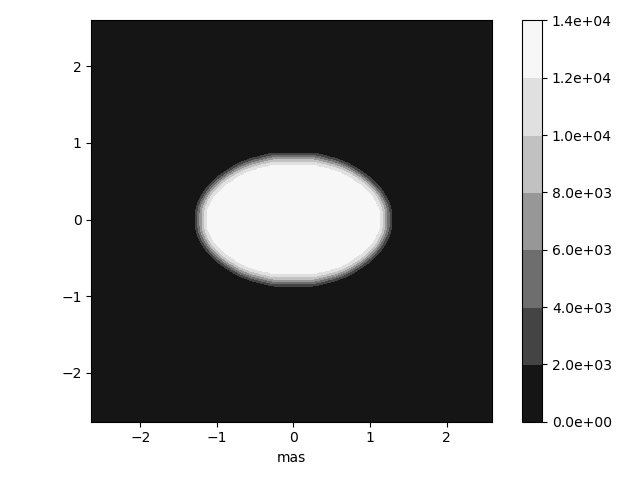
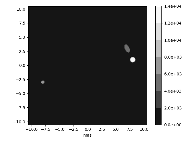
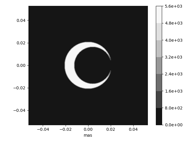
Figure 1: Example sources with effective temperature in K. See the last part of Section 1 for details.

There is a wealth of possible targets for next-generation interferometers (see Figure 10 of Dravins et al., 2013) but as illustrative examples we will consider three simple models consisting of blackbody sources in simple shapes. There are shown in Figure 1.

• First and simplest we have an ellipse of $\rm 2.4\,mas\times 1.6\,mas$ at $T_{\rm eff}=12500\rm\,K$, which approximates Achernar. This star was actually observed by Hanbury Brown et al. (1974) but without allowing for its rotational flattening, and hence measuring only a mean angular diameter. The flattening was measured by Domiciano de Souza et al. (2003) using Michelson-type interferometry.

• Next we have a three-component source approximating the Algol system, also based on reconstructions from Michelson-type interferometry (Zavala et al., 2010; Baron et al., 2012).

• Then we have a crescent source at $T_{\rm eff}=5000\rm\,K$, which does not represent any particular object but is reminiscent of two kinds of interesting systems. The angular size and pattern roughly mimics the M87 black hole (cf. Kamruddin & Dexter, 2013) though the brightness at optical wavelengths is totally speculative. Alternatively, we can imagine a subdwarf star some tens of pc away, with a giant planet in transit.

These systems are shown in Figure 1. We choose the frequency as the peak of the visible range ($\nu=540\rm\,THz$ or $\lambda=555\rm\,nm$). In the course of this paper we will compute the expected signal and noise for each of these systems.

2 Transient interference

In optics, coherent light produces interference, whereas incoherent light simply adds. Coherent vs incoherent is, however, not a dichotomy. Incoherent light filtered to a narrow band becomes partially coherent, and produces transient interference effects, which are only detectable with ultra-fast intensity measurements. This fact is the heart of the Hanbury Brown and Twiss effect, and the basis of intensity interferometry, but conventionally it is stated in terms of correlations and bunching. Here we will show that HBT can be considered as an extension of classical diffraction.

We will assume that (i) ordinary light is equivalent to a superposition of many lasers over a range of frequencies, and (ii) the classical intensity, suitably normalised, corresponds to the probability of detecting photons.

2.1 Brightness

Consider a channel in which light is filtered to a narrow band of width $\Delta\nu$ around a frequency $\nu$, and to a single polarisation state. There can be an independent channel for the orthogonal polarisation, and further channels at other frequencies, but let us consider this one channel. In this channel, let $|S({\bf\Omega})|^{2}\,\Delta\nu$ be the photon flux coming from direction ${\bf\Omega}$ on the sky. $|S({\bf\Omega})|^{2}$ will have units of photons $\rm m^{-2}\,sr^{-1}\,s^{-1}\,Hz^{-1}$. In particular

$$|S({\bf\Omega})|^{2}=\frac{\nu^{2}/c^{2}}{e^{h\nu/(kT({\bf\Omega}))}-1}$$ (1)

corresponds to a blackbody source with a temperature map of $T({\bf\Omega})$. Even if the source is not blackbody, Eq. (1) can still be used within a narrow band to give the photon flux in terms of an effective temperature.

Integrating over the source, let us write

$$\Phi=\int|S({\bf\Omega})|^{2}\,d^{2}{\bf\Omega}$$ (2)

for the photons $\rm m^{-2}\,s^{-1}\,Hz^{-1}$ coming from the source. The quantity $\Phi$ is a spectral photon flux, and is sometimes called the count degeneracy (see, e.g., Goodman, 2015).

Brightness in janskys or optical magnitudes can be replaced by $\Phi$. To do so, note first that the energy flux in a band (including both polarisations) will be $2h\nu\,\Delta\nu\,\Phi$. Hence $2h\nu\,\Phi$ will be the spectral flux density in $\rm W\,m^{-2}\,Hz^{-1}$. (Recall that $1\rm\,Jy$ is $10^{26}$ of this unit.) In terms of AB magnitudes we have

$$2h\nu\,\Phi=10^{-22.44-{\rm AB}/2.5}\rm\;W\,m^{-2}\,Hz^{-1}$$ (3)

This can be rearranged and rounded to the convenient expression

$$\Phi\approx 10^{-4-{\rm AB}/2.5}\frac{\lambda}{1\mu\rm m}{\rm\;m^{-2}}$$ (4)

The three example systems in Figure 1 have

$$\Phi=\left\{\begin{matrix}3.1\times 10^{-5}\\ 6.0\times 10^{-6}\\ 1.8\times 10^{-10}\\ \end{matrix}\right\}\hbox{photons}\ \rm m^{-2}\,s^{-1}\,Hz^{-1}$$ (5)

respectively.

The product $A\,\Phi$, where $A$ is an effective detector area (that is, light-collecting area times system throughput and detector efficiency), will be important later.

2.2 Complex amplitude

If the source were coherent and had a monochromatic frequency $\nu$, we could write

$$S({\bf\Omega})\,e^{2\pi i\,\nu t}$$ (6)

for the probability amplitude of a photon to come from direction ${\bf\Omega}$. The probability amplitude at a location ${\bf x}$ on the ground could be written as

$$\phi({\bf x})\,e^{2\pi i\,\nu t}$$ (7)

which corresponds to a brightness distribution $|\phi({\bf x})|^{2}$ on the ground. We will assume that ${\bf\Omega}$ is always a small solid angle, and further that it is near the zenith. For sources not at zenith one needs to apply a standard rotation (given in Appendix A) to ${\bf x}$.

The two amplitudes will be related by the classical Fraunhofer diffraction formula

$$\phi({\bf x})\propto\int e^{2\pi i\,(\nu/c)\,{\bf x}\cdot{\bf\Omega}}\,S({\bf\Omega})\,d^{2}{\bf\Omega}$$ (8)

with the proportionality constant chosen to satisfy

$$\left\langle\,|\phi({\bf x})|^{2}\right\rangle=\Phi$$ (9)

The proportionality constant is given in Eq. (61) in Appendix B.

2.3 Narrowband light

Let us now consider an incoherent source filtered to a narrow band around $\nu$, giving a frequency spectrum $W(\nu^{\prime})$. We have already used the bandwidth $\Delta\nu$. Let us now define it more precisely as

$$\Delta\nu=\int\!W(\nu^{\prime})\,d\nu^{\prime}=\int\!W^{2}(\nu^{\prime})\,d\nu^{\prime}$$ (10)

which also fixes the normalisation of the bandpass $W(\nu^{\prime})$. Next, let us introduce

$$\gamma(t)=\frac{1}{\Delta\nu}\int e^{2\pi i\,(\nu^{\prime}-\nu)t}\,W(\nu^{\prime})\,d\nu^{\prime}$$ (11)

which is a shifted Fourier transform of $W(\nu^{\prime})$. We then define the time scale

$$\Delta\tau=\int\!|\gamma(t)|^{2}\,dt$$ (12)

which we will call the coherence time. As we will see below, the coherence time is an indicator of how long Fraunhofer diffraction patterns persist. The Parseval relation corresponding to Eq. (11) implies

$$\Delta\tau=(\Delta\nu)^{-1}$$ (13)

To take an example, suppose we have a narrowband filter of $\Delta\lambda=1\rm\,nm$ around $\lambda=555\rm\,nm$. The coherence time will then be $\Delta\tau=\lambda^{2}/(c\Delta\lambda)\approx 1\rm\,ps$.

For narrowband light, the complex amplitude (6) on the sky will be replaced by

$$|S({\bf\Omega})|\;e^{i\alpha({\bf\Omega})}\times\frac{1}{\Delta\nu}\int e^{2\pi i\,\nu^{\prime}t}\,W(\nu^{\prime})\,d\nu^{\prime}$$ (14)

where $\alpha({\bf\Omega})$ is an initial phase, which is randomly different across the source. The ground amplitude (7) is proportional to

$$|S({\bf\Omega})|\;e^{i\alpha({\bf\Omega})}\times\frac{1}{\Delta\nu}\int e^{2\pi i(\nu^{\prime}/c)\,{\bf x}\cdot{\bf\Omega}}$$ (15)

$$e^{2\pi i\,\nu^{\prime}t}\,W(\nu^{\prime})\;d\nu^{\prime}\,d^{2}{\bf\Omega}$$

We assume $|\nu^{\prime}-\nu|\ll\nu$ and replace

$$e^{2\pi i(\nu^{\prime}/c)\,{\bf x}\cdot{\bf\Omega}}\rightarrow e^{2\pi i(\nu/c)\,{\bf x}\cdot{\bf\Omega}}$$

because there is no multiplication by $t$. Then the sky amplitude can be written as

$$S({\bf\Omega},t)\,e^{2\pi i\,\nu t}$$ (16)

where

$$S({\bf\Omega},t)=|S({\bf\Omega})|\;e^{i\alpha({\bf\Omega})}\times\gamma(t)$$ (17)

and the ground amplitude can be written as

$$\phi({\bf x},t)\,e^{2\pi i\,\nu t}$$ (18)

where

$$\phi({\bf x},t)\propto\int e^{2\pi i\,(\nu/c)\,{\bf x}\cdot{\bf\Omega}}\,S({\bf\Omega},t)\,d^{2}{\bf\Omega}$$ (19)

Eqs. (17) and (19) describe Fraunhofer diffraction with a slow time dependence. We see that a small spread in frequency around $\nu$ produces a slow variation in the brightness distribution $|\phi({\bf x},t)|^{2}$ on the ground. The larger the frequency spread, the faster the brightness will vary.

The photon flux on the ground is given by

$$|\phi({\bf x},t)|^{2}\;\Delta\nu\quad\hbox{or}\quad|\phi({\bf x},t)|^{2}\;(\Delta\tau)^{-1}$$ (20)

and $|\phi({\bf x},t)|^{2}$ nominally has units of photons $\rm s^{-1}\,m^{-2}\,Hz^{-1}$. It is more useful, however, to think of $|\phi({\bf x},t)|^{2}$ as photons $\rm m^{-2}$ per coherence time. Widening the bandpass will increase the photon flux, but the number of photons per unit area within a coherence time will remain the same. This fact will be important when we consider signal and noise.

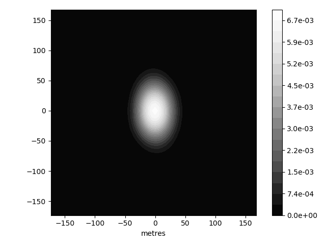
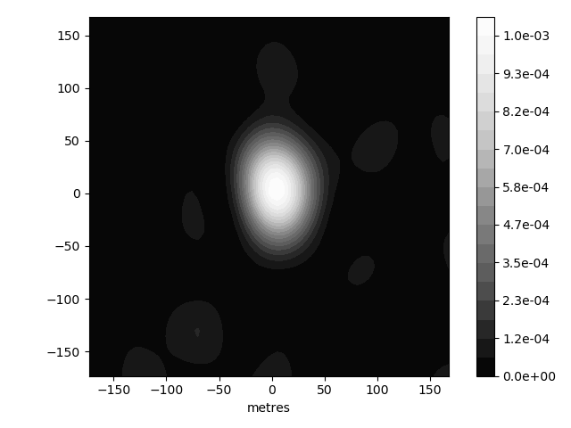
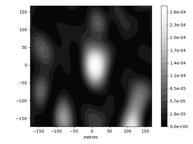
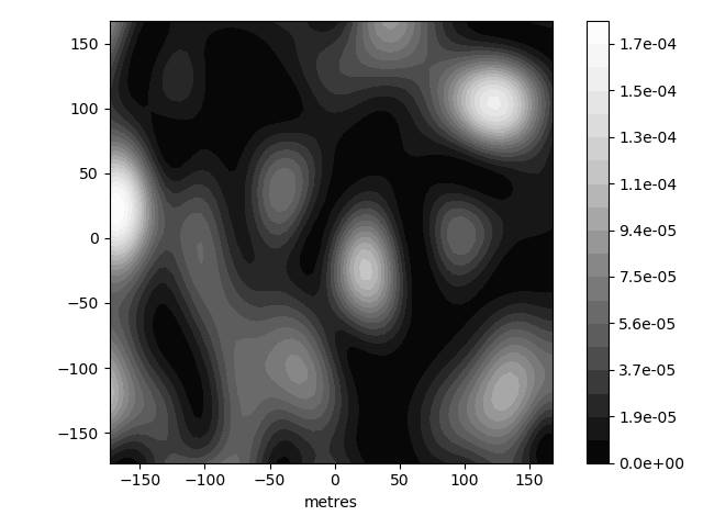
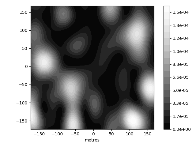
Figure 2: Simulation of decoherence of an initially coherent interference pattern. Shown is the ground brightness $|\phi({\bf x},t)|^{2}$ in photons $\rm m^{-1}$ per coherence time for the Achernar-like example source. Panels (in reading order, from top right to bottom left) are at $t=\Delta\tau,\dots,5\Delta\tau$. The frequency band is Lorentzian, and initial peak fades exponentially, as expected from Eq. (22).

2.4 Decoherence

As an example of a spectral bandpass, consider

$$W(\nu^{\prime})=\frac{2}{1+(2\pi\,\Delta\tau(\nu^{\prime}-\nu))^{2}}$$ (21)

which one can verify satisfies the normalisation (10). Physically, it is a Lorentzian spectrum with an arbitrary phase factor depending on ${\bf\Omega}$. For this spectrum we can then work out

$$S({\bf\Omega},t)=|S({\bf\Omega})|\exp\left(-\left|\frac{t}{\Delta\tau}-\frac{\alpha({\bf\Omega})}{2\pi}\right|\right)$$ (22)

which describes a flickering source: pulses rise at different ${\bf\Omega}$ at random times, and then fade exponentially, while the diffraction pattern on the ground flickers accordingly. Integrating, we can verify

$$\int|S({\bf\Omega},t)|^{2}\,dt=\Delta\tau\,|S({\bf\Omega})|^{2}$$ (23)

as implied by Eq. (17) above.

We can think of the source as the sum of many lasers with slightly different frequencies, the frequencies being distributed according to the Lorentzian (21). For simulations we set the phase of all frequency components to 0 at $t=0$. Thus the source is coherent at $t=0$, but as time passes the frequency differences make the source incoherent.

Figure 2 illustrates this decoherence. The figure shows $|\phi({\bf x},t)|^{2}$ from the Achernar-like source at $t=0,\Delta\tau,\ldots,5\Delta\tau$. At $t=0$ there is a single diffraction peak. The peak remains till $t=3\Delta\tau$ but its intensity fades as $e^{-2t/\Delta\tau}$ as expected from Eq. (22). By the last panel $t=5\Delta\tau$ the original diffraction peak is gone but many new peaks have appeared. This panel is typical of $|\phi({\bf x},t)|^{2}$ for incoherent light. In real life, we are never close to a coherent epoch for astronomical sources, so the scenario in this figure is completely artificial. For the following figures we will consider only random, hence incoherent, epochs. Setting $t\gg\Delta\tau$ in Eq. (24) below ensures that.

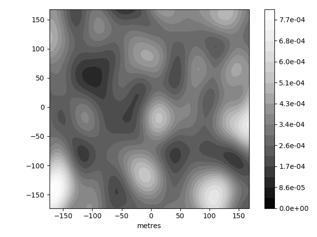
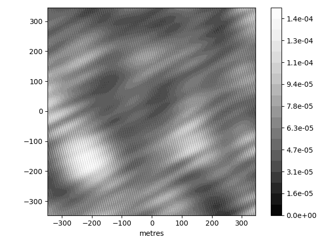
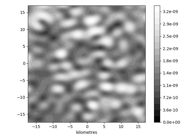
Figure 3: Transient interference patterns $X({\bf x},\Delta t=10\Delta\tau)$ in photons $\rm m^{-2}$ (see Eq. 24) for the three example sources from Figure 1.

2.5 Transient intensity

Although the intensity pattern on the ground changes completely within $5\Delta\tau$, it does not average out to uniform within that time. Consider now the expected photons $\rm m^{-2}$ over a time slice $\Delta t$ following time $t$. Call this $X({\bf x},\Delta t)$ for photon exposure (there is no standard name). We have

$$X({\bf x},\Delta t)=\Delta\nu\int_{t}^{t+\Delta t}|\phi({\bf x},t^{\prime})|^{2}\,dt^{\prime}$$ (24)

with $\Delta\nu=1/\Delta\tau$ as before. The uncertainty principle requires

$$\Delta t>\Delta\tau\quad\hbox{(typically $\Delta t\gg\Delta\tau$)}.$$ (25)

Figure 3 shows $X({\bf x},\Delta t=10\Delta\tau)$ for each of our example sources. (The three panels shown are 8-fold, 16-fold, and 4-fold zooms of the full simulations.) As can be read off from Figure 3, a bright blob is expected to yield less than one photon over a time interval $10\Delta\tau$. Integrating for many $\Delta\tau$ longer will not help trace the blobs, because the pattern keeps changing. The patterns in the simulation are thus too faint to be photographed.

Although unobservable with ordinary light, patterns similar to Figure 3 can be observed in laboratory experiments with pseudo-thermal (or quasi-thermal) light, which is light with an adjustable coherence time, produced say by moving ground glass across a coherent source. Some early but very nice examples appear in Martienssen & Spiller (1964).

2.6 Correlation

The transient patterns in Figure 3 clearly do contain information about the source map $|S({\bf x})|^{2}$ but in a highly distorted form. We now see how to extract that information.

Consider the product $\phi({\bf x}_{1},t)\,\phi^{*}({\bf x}_{2},t)$ which represents the instantaneous correlation between the amplitudes at two points on the ground. Note that complex amplitudes averages to zero, hence there is no constant term to subtract in the correlation. From the Fraunhofer diffraction formula (19) we see that the instantaneous correlation will be an integral over ${\bf\Omega}$ and ${\bf\Omega}^{\prime}$ with the integrand containing factors of $S({\bf\Omega},t)\,S^{*}({\bf\Omega}^{\prime},t)$. Because the light is chaotic, over long times the latter factors tend to cancel if ${\bf\Omega}\neq{\bf\Omega}^{\prime}$, and only $|S({\bf\Omega},t)|^{2}$ contributes. This fact is essentially the van Cittert-Zernike theorem, which has many interesting consequences (and not only for light waves — see Knox et al., 2010). The consequence of interest here is that the time-averaged correlation simplifies to

$$\langle\,\phi({\bf x}_{1},t)\,\phi^{*}({\bf x}_{2},t)\rangle\propto\int e^{2\pi i\,(\nu/c)\,({\bf x}_{1}-{\bf x}_{2})\cdot{\bf\Omega}}$$ (26)

$$\left\langle\,|S({\bf\Omega},t)|^{2}\right\rangle\,d^{2}{\bf\Omega}$$

Let us write the time average of the right-hand side of (26) as $V({\bf x}_{1}-{\bf x}_{2})$, with the normalisation $V(0)=1$. That is, $V({\bf x})$ is the spatial Fourier transform of the source intensity (not the source amplitude), with any source flickering time-averaged out. The time average of Eq. (26) is then

$$\frac{\langle\phi_{1}\,\phi_{2}^{*}\rangle}{\sqrt{\left\langle\,|\phi_{1}|^{2}\right\rangle\,\left\langle\,|\phi_{2}|^{2}\right\rangle}}=V_{12}$$ (27)

using the abbreviated notation $\phi_{1}\equiv\phi({\bf x}_{1},t)$, $\phi_{2}\equiv\phi({\bf x}_{2},t),V_{12}\equiv V({\bf x}_{1}-{\bf x}_{2})$. The physical meaning of this equation is that the time-averaged amplitude correlation on the ground is given by the normalised spatial Fourier transform of the source brightness.

The quantity $V({\bf x})$ is known as the complex visibility, and interferometry is all about measuring as much as possible of $V({\bf x})$. The difficulty is that measuring $\phi({\bf x}_{1},t)\,\phi^{*}({\bf x}_{2},t)$ requires controlling the optical path difference between ${\bf x}_{1}$ and ${\bf x}_{2}$ to sub-wavelength precision.

Intensity interferometry adopts a different strategy. First we note, that as we have seen from Figures 2 and 3, $|\phi({\bf x},t)|^{2}$ varies on the comparatively slow time scale of $\Delta\tau$. This makes the time average $\left\langle\,|\phi_{1}|^{2}\,|\phi_{2}|^{2}\right\rangle$ measurable without requiring sub-wavelength precision. We are then helped by an identity variously known as Isserlis’ theorem and Wick’s theorem. Of interest here is the case expressing $\langle\phi_{1}\ldots\phi_{N}\,\phi_{N}^{*}\ldots\phi_{1}^{*}\rangle$ in terms of products $\langle\phi_{m}\,\phi_{n}^{*}\rangle$ (see e.g., Eq. 10.27 in Glauber, 1963). The simplest instance is

$$\langle\phi_{1}\,\phi_{1}^{*}\,\phi_{2}\,\phi_{2}^{*}\rangle=\langle\,|\phi_{1}|^{2}\rangle\langle\,|\phi_{2}|^{2}\rangle+\left|\langle\phi_{1}\,\phi_{2}^{*}\rangle\right|^{2}$$ (28)

relating the intensity at two points to the visibility. Rearranging, we have

$$\frac{\left\langle\,|\phi_{1}|^{2}\,|\phi_{2}|^{2}\right\rangle}{\left\langle\,|\phi_{1}|^{2}\right\rangle\left\langle\,|\phi_{2}|^{2}\right\rangle}-1=|V_{12}|^{2}$$ (29)

As we see, correlating intensity at two points loses the phase information in $V_{12}$. The transient interference pattern contains more information, which could in principle be recovered by higher-order correlation. In particular, three-point intensity correlation includes a dependence on

$$\mathop{\rm Re}\big{[}\,V({\bf x}_{1}-{\bf x}_{2})\;V({\bf x}_{2}-{\bf x}_{3})\;V({\bf x}_{3}-{\bf x}_{1})\,\big{]}$$ (30)

(see e.g., Wentz & Saha, 2015). Still higher orders also possible (Fontana, 1983; Malvimat et al., 2014).

2.7 Summary

In this section, we have considered three forms of optical interference. Let us summarise these.

First we have Fraunhofer diffraction, which we write concisely as follows.

$$\phi ={\cal F}(S)$$ (31)

$$|\phi|^{2} ={\cal F}(S\circ S^{*})\vrule width=0.0pt,height=15.0pt$$

Here ${\cal F}$ denotes a Fourier transform, and expressions with $\circ$ are auto-correlations. The complex amplitude $\phi({\bf x})$ on the ground is the Fourier transform of the complex amplitude $S({\bf\Omega})$ of the source in the sky. If sources were coherent (if phases on different parts of the source were correlated) we would get interference fringes on the ground. But phases on the source are not correlated, hence $S\circ S^{*}$ is chaotic. The corresponding intensity $|\phi|^{2}$ on the ground is also chaotic, and time-averages to uniform illumination. This is illustrated in Figures 2 and 3.

Astronomical Michelson interferometry makes use of the van Cittert-Zernike theorem

$$\phi\circ\phi^{*}={\cal F}\left(\,|S|^{2}\right)\\$$ (32)

which as written here can be considered a corollary of the Fraunhofer diffraction integral. The source can be incoherent, and there are no interference fringes in $|\phi|^{2}$. Instead, fringes in $\phi\circ\phi^{*}$ are observable if phase coherence can be maintained across the telescope.

Finally we have intensity interferometry, which actually works because the source is not coherent, and the phase in $\phi$ is chaotic. Complex fields with random phases have the property that

$$|\phi|^{2}\circ|\phi|^{2}=|\phi|^{4}+|\phi\circ\phi^{*}|^{2}$$ (33)

and by exploiting this, $|\phi\circ\phi^{*}|^{2}$ can be inferred from intensity correlation without the need for phase coherence. The intensity patterns in Figure 3 are chaotic, but their auto-correlations are well-behaved. We will see this below in Figure 4.

In the next section, we will be especially concerned with $|V|$ and $\Phi$. These are nothing but the normalised form of $|\phi\circ\phi^{*}|$ and the normalisation factor respectively (see Eqs. 27 and 9).

3 Signal and noise

The apparatus in intensity interferometry is a light bucket, which counts photons over an effective area $A$ on the ground over some time-slice $\Delta t$. Let us write $N({\bf x})$ for the number of photons detected in a time-slice $\Delta t$. It will be usually 0, sometimes 1, but its expectation value will be

$$E\big{(}N({\bf x})\big{)}=A\,X({\bf x},\Delta t)$$ (34)

The basic observable in intensity interferometry is the time-averaged correlation between $N({\bf x}_{1})$ and $N({\bf x}_{2})$.

3.1 Photon correlation

Using the abbreviations $N_{1}$ and $N_{2}$

$$g_{12}\equiv\frac{\langle N_{1}N_{2}\rangle}{\langle N_{1}\rangle\langle N_{2}\rangle}-1$$ (35)

is the observable HBT correlation. This definition is a modified version of the formula (29) which gives $|V_{12}|^{2}$. A modification is required because in practice $\Delta t\gg\Delta\tau$, and HBT-correlated counts only occur within $\sim\Delta\tau$ of each other (before the transient interference pattern changes). Let us divide a time interval $\Delta t$ into $\Delta t/\Delta\tau$ time-slices of duration $\Delta\tau$ each, and approximate the light as being perfectly coherent within a time slice and completely incoherent between different time slices. The expected number of counts in a coherence time is $A\,\Phi$. The number of HBT correlated counts in $\Delta t$ will be

$$\langle N_{1}N_{2}\rangle-\langle N_{1}\rangle\langle N_{2}\rangle\approx(\Delta t/\Delta\tau)\;(A\,\Phi)^{2}\;|V_{12}|^{2}$$ (36)

whereas the total correlated counts will be

$$\langle N_{1}\rangle\langle N_{2}\rangle=(\Delta t/\Delta\tau)^{2}\;(A\,\Phi)^{2}$$ (37)

Together these give

$$g_{12}\approx\frac{\Delta\tau}{\Delta t}\,|V_{12}|^{2}$$ (38)

which is the observable correlation in intensity interferometry. Measuring the correlation with detectors close together will give $g(0)$ which is $\approx\Delta\tau/\Delta t$ since $V(0)=1$ by definition. The precise proportionality factor here will depend on the details of the frequency bandpass and time response of the photon detectors.

The instruments in first-generation intensity interferometry did not count photons explicitly. Instead, there were currents proportional to the photon counts, and the currents were correlated in hardware. In the definition (35) of $g_{12}$ it does not matter whether we use counts or intensities. Present-day technology, on the other hand, uses digitised signals from individual photon detections. This makes is interesting to consider variants of $g_{12}$ that are meaningful for photons counts but not for intensities. In the following sections, we consider two such variants.

3.2 A scaled correlation

Consider the quantity

$$h_{12}\equiv\frac{\langle N_{1}N_{2}\rangle-\langle N_{1}\rangle\langle N_{2}\rangle}{\sqrt{\langle N_{1}\rangle\langle N_{2}\rangle}}$$ (39)

which is the correlation times the geometric mean of counts in a time slice. Referring back to Eqs. (37) and (38) and noting that the average number of counts in a detector is $A\,\Phi$, we have

$$h({\bf x})\approx A\,\Phi\,|V({\bf x})|^{2}$$ (40)

where $A$ is understood as the geometric mean of the effective areas. Comparing with Eqs. (38) and (37) we can see that $h_{12}$ has the interpretation of signal-to-noise (SNR) per data point. Of course, $h_{12}$ is really an upper limit on the achievable SNR. The actual SNR will be lower, because of additional noise sources. We will call $h({\bf x})$ the scaled correlation.

It may be that one is interested in the difference of two cases, such as the on-transit and off-transit epochs of an exoplanetary system (cf. Fig. 11 of Dravins & Lagadec, 2014). For such situations, we define a differential signal which still has the interpretation of SNR per data point. Let us define

$$\sigma_{A}\equiv h_{A}(0)$$ (41)

which is approximately the numerator of Eq. (39) and hence can be interpreted as the noise level. Analogously, $\sigma h({\bf x})$ can be interpreted as the signal. Then the difference in signal between two cases, scaled by the combined noise, will be

$$\Delta h=\frac{\sigma_{A}h_{A}-\sigma_{B}h_{B}}{\sqrt{\sigma_{B}^{2}+\sigma_{B}^{2}}}$$ (42)

where the subscripts refer to the two cases.

3.3 Properties of the scaled correlation

The scaled correlation $h({\bf x})$ is a small number which gets measured once per time-slice $\Delta t$, with a noise of unity from photon statistics. Over a long observation, the noise falls to $(\Delta t/t_{\rm obs})^{1/2}$. The NSII used $\Delta t=\rm 10\,ns$. Nowadays, $\Delta t=\rm 1\,ns$ is common and $\Delta t=\rm 0.1\,ns$ is possible (Pilyavsky et al., 2017). Thus, one night of observing could have $>10^{14}$ data points. The vast majority of these data points may have zero photons detected, but with so many data points $h\sim 10^{-6}$ would be measurable. Once $h({\bf x})$ is measured, $V({\bf x})$ will also be determined, as the two differ only in normalisation.

Interestingly, the bandwidth (and hence the coherence time) does not appear in the scaled correlation. This is because decreasing the bandwidth decreases the photon count, but correspondingly increases the coherence time, so $A\Phi$ remains the same. With SNR not depending on bandwidth, it is possible to split a narrow spectral band into multiple narrower bands, each having the same SNR as before. (It is understood that the coherence time $\Delta\tau$ is shorter than the detector time resolution $\Delta t$. Narrowing the bandpass will help only till $\Delta\tau\approx\Delta t$.) Some experimental detectors (see Horch et al., 2016) have multiple simultaneous channels observing in separate narrow spectral bands. In a laboratory setting kilo-pixel photon detection with $\Delta t<1\rm\,ns$ has been achieved (Wollman et al., 2019). If the latter are some day installed on intensity interferometers, an observing night would yield $\sim 10^{17}$ data points, and then even $h=10^{-8}$ would be viable.

In $\Phi$ we have considered only one polarisation channel. Detector designs so far do not separate the polarisation channels. When this is done, the two polarisation states behave like two unseparated spectral channels: both signal and noise double, leaving the SNR the same. If photons in two polarisation channels are correlated separately, that should give two simultaneous measurements with the same SNR.

That $h$ is independent of both $\Delta t$ and $\Delta\tau$ is something peculiar to two-point HBT. For $N$-point correlations the scaled correlation is

$$h^{(N)}\approx V^{(N)}\times(A\Phi)^{N/2}\left(\frac{\Delta\tau}{\Delta t}\right)^{N/2-1}$$ (43)

(cf. Malvimat et al., 2014). We will not discuss higher-order HBT in this paper, but just remark here that it is much more difficult to observe, because $\Phi$ is raised to a higher power in the SNR.

3.4 A correlation density

Another possible variant of the correlation is

$$f({\bf x}_{2}-{\bf x}_{1})\equiv\frac{\langle X({\bf x}_{1})X({\bf x}_{2})\rangle}{\langle X\rangle}-{\langle X\rangle}$$ (44)

having dimensions of inverse area. We may call the correlation density. Clearly $f({\bf x})=\langle X\rangle\,g({\bf x})$ and hence

$$f({\bf x})\approx\Phi\;|V({\bf x})|^{2}$$ (45)

which depends only on the source. The correlation density is convenient when we do not have a particular observational setup in mind, and wish to assess what instrumentation would be needed to resolve a given source. Examples follow.

3.5 Additional noise sources

Beyond the essential statistics of photons, any practical intensity interferometer will have additional sources of noise. Here we just mention three, which are considered in simulations by Rou et al. (2013).

First, there is extra light which produces noise without signal. Mirrors that are not of optical quality have a roughness that produces a large point spread function. For Cherenkov telescopes, the point spread functions are an arc-minute or more (see e.g., Tayabaly et al., 2015) and this naturally lets in extra light from the night sky. The SNR per data point will be

$$\frac{A\,\Phi}{1+\Phi^{x}\!/\Phi}\,|V({\bf x})|^{2}$$ (46)

where $\Phi^{x}$ is the spectral photon flux of the extraneous light. If $\Phi^{x}\ll\Phi$ the total observing time needed will be $\propto\Phi^{-2}$. If $\Phi^{x}\gg\Phi$ the observing time becomes $\propto\Phi^{-4}$. Hence, intensity interferometry would be effectively infeasible for sources fainter than the night sky within the point spread function.

Second, optical-path differences across the collecting mirror and elsewhere in the optics may reduce the effective $\Delta t$. This is especially a problem if a solar-furnace design is used for the collecting mirrors, because solar furnaces have no use for isochronous optical paths.

Third, the response of the photon detectors may not be uniform. Hanbury Brown & Twiss (1957) in their Eq. (3.62) included a model for non-uniform photo-electric response in their detectors, but current detectors may need a different model.

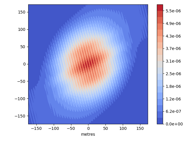
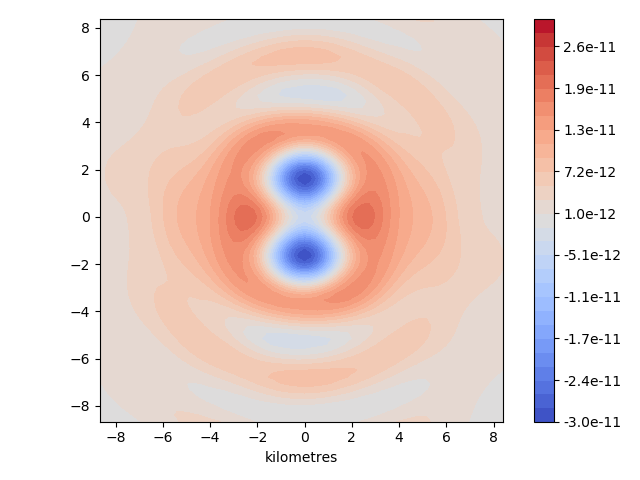
Figure 4: Correlation density in coincidences $\rm m^{-2}$ per coherence time for the three example sources. The upper and middle panels show $f({\bf x})$ from Eq. (44) while the lower panel shows $\Delta f({\bf x})$ from Eq. (47).

3.6 The example systems

Figure 4 shows the simulated $f({\bf x})$ for our three example sources, obtained from the simulated transient interference patterns. The simulated correlation $g({\bf x})$ is not shown, since it only differs in the normalisation, but we have verified that $g(0)\simeq\Delta\tau/\Delta t$ in all cases. Figure 4 could also have been generated Eq. (45) without bothering with simulations of $X({\bf x})$, but it is nice to verify that simulating the transient interference gives the expected result.

Note that the three panels in Figure 4 are zoomed twofold compared to Figure 3.

For Achernar, we see that a collecting area of $0.1\rm\,m^{2}$ with a throughput of order 50% would bring $h\sim 10^{-6}$. In the optimistic scenario that this level of throughput is achieved, and there are no other significant sources of noise, two amateur-grade telescope with high-end photon counters and correlator would be enough to measure the angular size and ellipticity of Achernar.

Algol represents a higher level of difficulty, both because it is fainter and because there are three stars. Here the adaptation of Cherenkov telescopes for intensity interferometry currently under development (e.g., Kieda et al., 2019) are a promising venue. With mirror areas of $>10\rm\,m^{2}$ and baselines of up to $100\rm\,m$, adequate SNR would be achievable.

For the crescent source, following the discussion around Eq. (42), we show the differential quantity

$$\Delta f({\bf x})={\textstyle\frac{1}{\sqrt{2}}}(f({\bf x})-\bar{f}({\bf x}))$$ (47)

where $\bar{f}({\bf x})$ refers to a disc source with the same radius and brightness. For a transiting exoplanet, $\bar{f}({\bf x})$ would correspond to an observable source, otherwise it is just a notional reference. Resolving the crescent source would not be possible in the near future. Cherenkov telescopes offer the prospect of $10^{3}\rm\,m^{2}$ of collecting area and baselines of up to $2\rm\,km$. The baseline is enough to resolve the crescent features, but the collecting area would bring the SNR to only $\sim 10^{-8}$ per data point, which is not feasible to work with as yet. But brighter sources of similar size are potential targets.

3.7 The inverse problem

Reconstructing the source brightness distribution $|S({\bf\Omega})|^{2}$ from incomplete information on $V({\bf x})$ is an archetypical inverse problem. In cases where there is a model for the source and only some parameter fitting is required (say measuring angular size and ellipticity), solving the inverse problem is not necessary. But for general sources the inverse problem will be important in intensity interferometry. From Eq. (32) it follows that

$$|\phi\circ\phi^{*}|^{2}={\cal F}\left(\,|S|^{2}\circ|S|^{2}\right)\,.$$ (48)

To help understand this relation, in Figure 5 we have taken $|V({\bf x})|^{2}$ for the Algol-like source and plotted the absolute value of its inverse Fourier transform. The result, which as we see has inversion symmetry, is not the original three-star source brightness $|S({\bf\Omega})|^{2}$, but is clearly somehow related to it. The figure illustrates the unavoidable information loss in intensity correlation. In practice, one would not have a complete map of $|V({\bf x})|^{2}$, so taking the inverse Fourier transform of $|V({\bf x})|^{2}$ is not a feasible reconstruction method. It is at best comparable to a dirty-map reconstruction in radio interferometry. However, algorithms for source reconstruction from intensity correlation (including three-point correlation if available) have been developed (Nuñez & Domiciano de Souza, 2015).

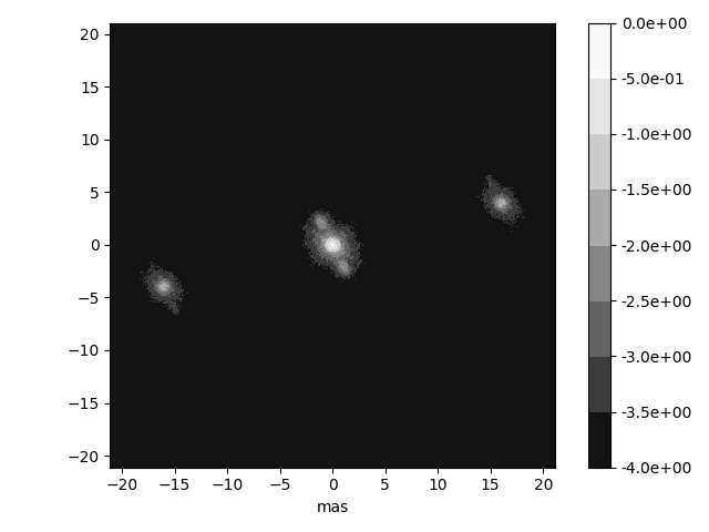
Figure 5: Dirty-map reconstruction of the Algol-like source (see subsection 3.7 for details). The scale is $\log_{10}$ with an arbitrary normalization.

4 Discussion

This paper is about a conceptual question: what really is being measured in intensity correlation? We argue that intensity interferometry can be thought of as measuring fringe sizes in a transient interference pattern which cannot itself be observed, because its bright fringes are sub-photon. The essential idea has always been implicit in the theory of HBT, just not made concrete, because numerically simulating transient interference patterns was not so easy when the theory was developed.

The notion of an interference pattern on the ground, even if transient, suggests an interesting possibility for situations that would currently be problematic. As an example, consider the Algol system, from which the smallest fringes are $<10\rm\,m$ apart in visible light (see the middle panel in Figures 3). Mirrors up to 17 m in diameter are already in use for intensity interferometry (Acciari et al., 2020) but too-large a light bucket would average out the small fringes. But suppose the light is collected and brought to a focus by a large mirror, and then re-collimated by a secondary mirror or lens. The result would be a miniature version of the interference pattern on the ground. Photon detection and correlation could be done on the miniaturised pattern, with the help of further optical elements. The relatively imprecise figuring of the large mirror will introduce optical-path errors of course, but these would be harmless if they are smaller than the detector time-resolution. Thus, it appears that a very large collecting mirror need not result in a loss of resolution.

A further possible application of the same basic idea would be turn solar power towers into intensity interferometers by night. Solar power towers (see e.g., Breeze, 2016) use a large number of freely-orientable flat mirrors (known as heliostats) to focus light to a furnace at the top of a tower. The optical path length is different for each heliostat, which seemingly precludes interferometry. But perhaps the light could be re-collimated by a suitable secondary mirror such that each heliostat has its own separate sub-beam, which could go to a detector specific to that heliostat, and then the detectors could be synchronised in software. There would still be a spread in optical paths across each heliostat, thus limiting the time-resolution $\Delta t$, but perhaps even that could be corrected for. But this is very speculative, so we will stop here.

Thanks to Subrata Sarangi for asking all the right questions that led to this work, and to Nolan Matthews and Nitu Rai for comments and corrections.

Appendix A Rotation of the baseline

The ${\bf x}$ vector in this paper is a plane nearly perpendicular to the line of sight, so that small-angle approximations are valid. In general, the ${\bf x}$ plane will not be the horizontal plane $(x_{\scriptscriptstyle\rm E},x_{\scriptscriptstyle\rm N})$, and a rotation of coordinates needs to be applied. The required rotation is

$$\begin{pmatrix}x\\ y\\ z\end{pmatrix}=R_{x}(\delta)\,R_{y}(h)\,R_{x}(-l)\begin{pmatrix}x_{\scriptscriptstyle\rm E}\\ x_{\scriptscriptstyle\rm N}\\ x_{\rm up}\end{pmatrix}$$ (49)

where

$$R_{x}(\delta)=\begin{pmatrix}1&0&0\\ 0&\cos\delta&-\sin\delta\\ 0&\sin\delta&\cos\delta\end{pmatrix}$$ (50)

and similarly for $R_{x}(-l)$ while

$$R_{y}(h)=\begin{pmatrix}\cos h&0&\sin h\\ 0&1&0\\ -\sin h&0&\cos h\end{pmatrix}$$ (51)

where $l$ is the latitude of the setup, $\delta$ is the declination and $h$ is the hour angle of the source. Expanding out the product (49) is equivalent to Eq. (7) from Dravins et al. (2013). The transformation is basically the same as in radio-interferometry, with our $(x,y,z)$ being equivalent to $(u,v,w)$ from radio-astronomy, multiplied by the wavelength.

Appendix B Numerical implementation

Given a source brightness $|S({\bf\Omega})|$, one can put down a spectrum $F({\bf\Omega},\nu^{\prime})$ and compute the corresponding $\phi({\bf\Omega},t)$ using equation (19). We now see how to implement this numerically.

B.1 FFT libraries

Numerical libraries provide efficient implementations of 2D Fourier transforms. On an $N\times N$ grid the forward and inverse Fourier transforms are given as follows.

$$\phi_{pq}= \sum_{m,n}\exp\left(2\pi i\,\frac{pm+qn}{N}\right)\,S_{mn}$$ (52)

$$S_{mn}=\frac{1}{N^{2}} \sum_{p,q}\exp\left(-2\pi i\,\frac{pm+qn}{N}\right)\,\phi_{pq}$$

The discrete Parseval relation

$$\sum_{m,n}\left|S_{mn}\right|^{2}=N^{-2}\sum_{p,q}\left|\phi_{pq}\right|^{2}$$ (53)

is automatically satisfied.

We could change the definition to put the $1/N^{2}$ factor in the forward transform, or have a $1/N$ factor in both the forward and the inverse transform. But the above is the standard definition used by numerical libraries, so let us stay with it.

B.2 Discretization

Let us discretize the sky and ground coordinates on grids of size $N\times N$. Let

$${\bf\Omega} =m\,\Delta s,\,n\,\Delta s$$ (54)

$${\bf x} =p\,\Delta b,\,q\,\Delta b$$

where $m,n,p,q$ are all integers in $0,\ldots,N-1$. The steps $\Delta s$ and $\Delta b$ are chosen such that

$$\Delta s\times\Delta b=\frac{c/\nu}{N}$$ (55)

because then

$$(\nu/c)\,{\bf x}\cdot{\bf\Omega}=\frac{pm+qn}{N}$$ (56)

which makes the FFT carry out the Fraunhofer diffraction formula.

The conventional definition (52) of the Fourier transform makes the normalisation of $S_{mn}$ and $\phi_{pq}$ a little tricky. We can choose $S_{mn}=S({\bf\Omega},t)$ or $\phi_{pq}=\phi({\bf x},t)$ but not both. We opt for the latter, and set

$$S_{mn}=\Delta s\;\frac{\nu/c}{\sqrt{e^{h\nu/(kT({\bf\Omega}))}-1}}\;e^{i\alpha({\bf\Omega})}$$ (57)

with $T({\bf\Omega})$ following the effective temperature map as in Figure 1. The phase $\alpha({\bf\Omega})$ we will set below. Substituting $S_{mn}$ in the discrete Parseval relation (53) gives

$$\frac{\nu^{2}/c^{2}}{e^{h\nu/(kT({\bf\Omega}))}-1}\sum_{m,n}(\Delta s)^{2}=N^{-2}\sum_{p,q}\left|\phi_{pq}\right|^{2}$$ (58)

If we now put

$$\phi_{pq}=\phi({\bf x})$$ (59)

the previous relation has the interpretation

$$\int|S({\bf\Omega})|^{2}d^{2}{\bf\Omega}=\left\langle|\phi({\bf x})|^{2}\right\rangle$$ (60)

which is what we want. Eq. (60) itself is a Parseval relation corresponding to

$$\phi({\bf x})={} (\nu/c)\,{\textstyle\left(\int d^{2}{\bf x}\right)^{1/2}}\,\times$$ (61)

$$\int e^{2\pi i\,(\nu/c)\,{\bf x}\cdot{\bf\Omega}}\,S({\bf\Omega})\,d^{2}{\bf\Omega}$$

And now we finally have the full form of Eq. (8). The proportionality factor (which we have not included in Eq. 8) is clearly unphysical, but that is just a consequence of small-angle approximations, and is harmless in practice.

B.3 The frequency band

It remains to set the phases $\alpha({\bf\Omega})$ in Eq. (57). We let

$$\alpha=2\pi(\nu^{\prime}-\nu)t$$ (62)

where $\nu^{\prime}$ is assigned randomly at each grid-point according to

$$\nu^{\prime}-\nu=\frac{\tan(\pi r)}{2\pi\Delta\tau}\qquad-\textstyle{\frac{1}{2}}<r<\textstyle{\frac{1}{2}}$$ (63)

where $r$ is uniformly random. This distributes $\nu^{\prime}$ according to $dr/d\nu^{\prime}$, which equals the frequency band (21) we wish to implement. This has $2\pi(\nu^{\prime}-\nu)$ within $[-1/\Delta\tau,1/\Delta\tau]$ half the time, but has tails extending much beyond this range.

References

- Abeysekara et al. (2020) Abeysekara, A. U., Benbow, W., Brill, A., et al. 2020, Nature Astronomy
- Acciari et al. (2020) Acciari, V. A., Bernardos, M. I., Colombo, E., et al. 2020, MNRAS, 491, 1540
- Akiyama et al. (2019) Akiyama, K., Alberdi, A., Alef, W., et al. 2019, ApJL, 875, L1
- Baron et al. (2012) Baron, F., Monnier, J. D., Pedretti, E., et al. 2012, ApJ, 752, 20
- Breeze (2016) Breeze, P. 2016, in Solar Power Generation, ed. P. Breeze (Academic Press), 35–40
- Domiciano de Souza et al. (2003) Domiciano de Souza, A., Kervella, P., Jankov, S., et al. 2003, A&A, 407, L47
- Dravins & Lagadec (2014) Dravins, D. & Lagadec, T. 2014, in Society of Photo-Optical Instrumentation Engineers (SPIE) Conference Series, Vol. 9146, Proc. SPIE, 91460Z
- Dravins et al. (2015) Dravins, D., Lagadec, T., & Nuñez, P. D. 2015, A&A, 580, A99
- Dravins et al. (2013) Dravins, D., LeBohec, S., Jensen, H., Nuñez, P. D., & CTA Consortium. 2013, Astroparticle Physics, 43, 331
- Fontana (1983) Fontana, P. R. 1983, Journal of Applied Physics, 54, 473
- Glauber (1963) Glauber, R. J. 1963, Physical Review, 131, 2766
- Gómez et al. (2016) Gómez, J. L., Lobanov, A. P., Bruni, G., et al. 2016, ApJ, 817, 96
- Goodman (2015) Goodman, J. 2015, Statistical Optics, Wiley Series in Pure and Applied Optics (Wiley)
- Hanbury Brown (1974) Hanbury Brown, R. 1974, The intensity interferometer: Its application to astronomy (Taylor and Francis)
- Hanbury Brown et al. (1974) Hanbury Brown, R., Davis, J., & Allen, L. R. 1974, MNRAS, 167, 121
- Hanbury Brown & Twiss (1954) Hanbury Brown, R. & Twiss, R. Q. 1954, Philosophical Magazine, 45, 663
- Hanbury Brown & Twiss (1956) Hanbury Brown, R. & Twiss, R. Q. 1956, Nature, 177, 27
- Hanbury Brown & Twiss (1957) Hanbury Brown, R. & Twiss, R. Q. 1957, Proceedings of the Royal Society of London Series A, 242, 300
- Haubois et al. (2019) Haubois, X., Norris, B., Tuthill, P. G., et al. 2019, A&A, 628, A101
- Horch et al. (2016) Horch, E. P., Weiss, S. A., Rupert, J. D., et al. 2016, in Proc. SPIE, Vol. 9907, Optical and Infrared Interferometry and Imaging V, 99071W
- Howell & Horch (2018) Howell, S. B. & Horch, E. P. 2018, Physics Today, 71, 78
- Kamruddin & Dexter (2013) Kamruddin, A. B. & Dexter, J. 2013, MNRAS, 434, 765
- Kieda et al. (2019) Kieda, D., Anton, G., Barbano, A., et al. 2019, in BAAS, Vol. 51, 227
- Kleppner (2008) Kleppner, D. 2008, Physics Today, 61, 8
- Knox et al. (2010) Knox, W. H., Alonso, M., & Wolf, E. 2010, Physics Today, 63, 11
- Labeyrie (1970) Labeyrie, A. 1970, A&A, 6, 85
- Malvimat et al. (2014) Malvimat, V., Wucknitz, O., & Saha, P. 2014, MNRAS, 437, 798
- Mandel et al. (1964) Mandel, L., Sudarshan, E. C. G., & Wolf, E. 1964, Proceedings of the Physical Society, 84, 435
- Mandel & Wolf (1965) Mandel, L. & Wolf, E. 1965, Reviews of Modern Physics, 37, 231
- Martienssen & Spiller (1964) Martienssen, W. & Spiller, E. 1964, American Journal of Physics, 32, 919
- Matthews et al. (2018) Matthews, N., Kieda, D., & LeBohec, S. 2018, Journal of Modern Optics, 65, 1336
- Nuñez & Domiciano de Souza (2015) Nuñez, P. D. & Domiciano de Souza, A. 2015, MNRAS, 453, 1999
- Ou (2017) Ou, Z.-Y. J. 2017, Quantum optics for experimentalists / Zhe-Yu Jeff Ou, Indiana University - Purdue University Indianapolis, USA. (World Scientific)
- Pilyavsky et al. (2017) Pilyavsky, G., Mauskopf, P., Smith, N., et al. 2017, MNRAS, 467, 3048
- Rivet et al. (2020) Rivet, J. P., Siciak, A., de Almeida, E. S. G., et al. 2020, MNRAS, 494, 218
- Rou et al. (2013) Rou, J., Nuñez, P. D., Kieda, D., & LeBohec, S. 2013, MNRAS, 430, 3187
- Rueckner & Peidle (2013) Rueckner, W. & Peidle, J. 2013, American Journal of Physics, 81, 951
- Tayabaly et al. (2015) Tayabaly, K., Spiga, D., Canestrari, R., et al. 2015, in Society of Photo-Optical Instrumentation Engineers (SPIE) Conference Series, Vol. 9603, Proc. SPIE, 960307
- Trippe et al. (2014) Trippe, S., Kim, J.-Y., Lee, B., et al. 2014, Journal of Korean Astronomical Society, 47, 235
- Weiss et al. (2018) Weiss, S. A., Rupert, J. D., & Horch, E. P. 2018, in Society of Photo-Optical Instrumentation Engineers (SPIE) Conference Series, Vol. 10701, Optical and Infrared Interferometry and Imaging VI, 107010X
- Wentz & Saha (2015) Wentz, T. & Saha, P. 2015, MNRAS, 446, 2065
- Wollman et al. (2019) Wollman, E. E., Verma, V. B., Lita, A. E., et al. 2019, Optics Express, 27, 35279
- Zampieri et al. (2016) Zampieri, L., Naletto, G., Barbieri, C., et al. 2016, in Proc. SPIE, Vol. 9907, Optical and Infrared Interferometry and Imaging V, 99070N
- Zavala et al. (2010) Zavala, R. T., Hummel, C. A., Boboltz, D. A., et al. 2010, ApJL, 715, L44
- Zmija et al. (2020) Zmija, A., Deiml, P., Malyshev, D., et al. 2020, Optics Express, 28, 5248