Iterative Refinement in the Continuous Space
for Non-Autoregressive Neural Machine Translation

Abstract

We propose an efficient inference procedure for non-autoregressive machine translation that iteratively refines translation purely in the continuous space. Given a continuous latent variable model for machine translation (Shu et al., 2020), we train an inference network to approximate the gradient of the marginal log probability of the target sentence, using only the latent variable as input. This allows us to use gradient-based optimization to find the target sentence at inference time that approximately maximizes its marginal probability. As each refinement step only involves computation in the latent space of low dimensionality (we use 8 in our experiments), we avoid computational overhead incurred by existing non-autoregressive inference procedures that often refine in token space. We compare our approach to a recently proposed EM-like inference procedure (Shu et al., 2020) that optimizes in a hybrid space, consisting of both discrete and continuous variables. We evaluate our approach on WMT’14 En$\rightarrow$De, WMT’16 Ro$\rightarrow$En and IWSLT’16 De$\rightarrow$En, and observe two advantages over the EM-like inference: (1) it is computationally efficient, i.e. each refinement step is twice as fast, and (2) it is more effective, resulting in higher marginal probabilities and BLEU scores with the same number of refinement steps. On WMT’14 En$\rightarrow$De, for instance, our approach is able to decode $6.2$ times faster than the autoregressive model with minimal degradation to translation quality (0.9 BLEU).

1 Introduction

Most neural machine translation systems are autoregressive, hence decoding latency grows linearly with respect to the length of the target sentence. For faster generation, several work proposed non-autoregressive models with sub-linear decoding latency given sufficient parallel computation (Gu et al., 2018a; Lee et al., 2018; Kaiser et al., 2018).

As it is challenging to precisely model the dependencies among the tokens without autoregression, many existing non-autoregressive models first generate an initial translation which is then iteratively refined to yield better output (Lee et al., 2018; Gu et al., 2019; Ghazvininejad et al., 2019). While various training objectives are used to admit refinement (e.g. denoising, evidence lowerbound maximization and mask language modeling), the generation process of these models is similar in that the refinement process happens in the discrete space of sentences.

Meanwhile, another line of work proposed to use continuous latent variables for non-autoregressive translation, such that the distribution of the target sentences can be factorized over time given the latent variables (Ma et al., 2019; Shu et al., 2020). Unlike the models discussed above, finding the most likely target sentence under these models requires searching over continuous latent variables. To this end, Shu et al. (2020) proposed an EM-like inference procedure that optimizes over a hybrid space consisting of both continuous and discrete variables. By introducing a deterministic delta posterior, it maximizes a proxy lowerbound by alternating between matching the delta posterior to the original approximate posterior (continuous optimization), and finding a target sentence that maximizes the proxy lowerbound (discrete search).

In this work, we propose an iterative inference procedure for latent variable non-autoregressive models that purely operates in the continuous space. Given a latent variable model, we train an inference network to estimate the gradient of the marginal log probability of the target sentence, using only the latent variable as input. At inference time, we find the target sentence that approximately maximizes the log probability by (1) initializing the latent variable e.g. as the mean of the prior, and (2) following the gradients estimated by the inference network.

We compare the proposed approach with the EM-like inference (Shu et al., 2020) on three machine translation datasets: WMT’14 En$\rightarrow$De, WMT’16 Ro$\rightarrow$En and IWSLT’16 De$\rightarrow$En. The advantages of our approach are twofold: (1) each refinement step is twice as fast, as it avoids discrete search over a large vocabulary, and (2) it is more effective, giving higher marginal probabilities and BLEU scores with the same number of refinement steps. Our procedure results in significantly faster inference, for instance giving $6.2\times$ speedup over the autoregressive baseline on WMT’14 En$\rightarrow$De at the expense of $0.9$ BLEU score.

2 Background: Iterative Refinement for Non-Autoregressive Translation

We motivate our approach by reviewing existing refinement-based non-autoregressive models for machine translation in terms of their inference procedure. Let us use $V,\>D,\>T$ and $L$ to denote vocabulary size, latent dimensionality, target sentence length and the number of refinement steps, respectively.

Most machine translation models are trained to maximize the conditional log probability $\log p(\bm{\mathrm{y}}|\bm{\mathrm{x}})$ of the target sentence $\bm{\mathrm{y}}$ given the source sentence $\bm{\mathrm{x}}$, averaged over the training data consisting of sentence pairs $\{(\bm{\mathrm{x}}_{n},\bm{\mathrm{y}}_{n})\}_{n=1}^{N}$. To find the most likely target sentence at test time, one performs maximum-a-posteriori inference by solving a search problem $\hat{\bm{\mathrm{y}}}=\text{argmax}_{\bm{\mathrm{y}}}\log p(\bm{\mathrm{y}}|\bm{\mathrm{x}}).$

2.1 Refinement in a Discrete Space

As the lack of autoregression makes it challenging to model the dependencies among the target tokens, most of the existing non-autoregressive translation models use iterative refinement to impose dependencies in the generation process. Various training objectives are used to incorporate refinement, e.g. denoising (Lee et al., 2018), mask language modeling (Ghazvininejad et al., 2019) and evidence lowerbound maximization (Chan et al., 2019; Gu et al., 2019). However, inference procedures employed by these models are similar in that an initial hypothesis is generated and then successively refined. We refer the readers to (Mansimov et al., 2019) for a formal definition of a sequence generation framework that unifies these models, and briefly discuss the inference procedure below.

By viewing each refinement step as introducing a discrete random variable $\bm{\mathrm{z}}_{i}$ (a $T\times V$-dimensional matrix, where each row is one-hot), inference with $L$ refinement steps requires finding $\bm{\mathrm{y}}$ that maximizes the log probability $\log p(\bm{\mathrm{y}}|\bm{\mathrm{x}})$.

$$\log p_{\theta}(\bm{\mathrm{y}}|\bm{\mathrm{x}})=\log\sum_{\bm{\mathrm{z}}_{1:L}}p_{\theta}(\bm{\mathrm{y}},\bm{\mathrm{z}}_{1:L}|\bm{\mathrm{x}})$$

$$=\log\sum_{\bm{\mathrm{z}}_{1:L}}\Big{(}p_{\theta}(\bm{\mathrm{y}}|\bm{\mathrm{z}}_{1:L},\bm{\mathrm{x}})\cdot\prod_{i=1}^{L}p_{\theta}(\bm{\mathrm{z}}_{i}|\bm{\mathrm{z}}_{<i},\bm{\mathrm{x}})\Big{)}$$

$$\geq\sum_{\bm{\mathrm{z}}_{1:L}}\Big{(}\log p_{\theta}(\bm{\mathrm{y}}|\bm{\mathrm{z}}_{1:L},\bm{\mathrm{x}})+\sum_{i=1}^{L}\log p_{\theta}(\bm{\mathrm{z}}_{i}|\bm{\mathrm{z}}_{<i},\bm{\mathrm{x}})\Big{)}.$$ (1)

As the marginalization over $\bm{\mathrm{z}}_{1:L}$ is intractable, inference for these models instead maximize the log joint probability with respect to $\hat{\bm{\mathrm{z}}}_{1:L}$ and $\bm{\mathrm{y}}$:

$$\log p_{\theta}(\bm{\mathrm{y}}|\hat{\bm{\mathrm{z}}}_{1:L},\bm{\mathrm{x}})+\,\,\sum_{i=1}^{L}\log p_{\theta}(\hat{\bm{\mathrm{z}}}_{i}|\hat{\bm{\mathrm{z}}}_{<i},\bm{\mathrm{x}}).$$

Approximate search methods are used to find $\hat{\bm{\mathrm{z}}}_{1:L}$ as $\hat{\bm{\mathrm{z}}}_{i}=\text{argmax}_{\bm{\mathrm{z}}_{i}}\log p_{\theta}(\bm{\mathrm{z}}_{i}|\hat{\bm{\mathrm{z}}}_{<i},\bm{\mathrm{x}}).$

2.2 Refinement in a Hybrid Space

Learning

On the other hand, Ma et al. (2019); Shu et al. (2020) proposed to use continuous latent variables for non-autoregressive translation. By letting the latent variables $\bm{\mathrm{z}}$ (of dimensionality $T\times D$) capture the dependencies between the target tokens, the decoder $p_{\theta}(\bm{\mathrm{y}}|\bm{\mathrm{z}},\bm{\mathrm{x}})$ can be factorized over time. As exact posterior inference and learning is intractable for most deep parameterized prior and decoder distributions, these models are trained to maximize the evidence lowerbound (ELBO) (Kingma and Welling, 2014; Wainwright and Jordan, 2008).

$$\log p_{\theta}(\bm{\mathrm{y}}|\bm{\mathrm{x}})\geq\operatorname*{\mathbb{E}}_{\bm{\mathrm{z}}\sim q_{\phi}}\Big{[}\log\frac{p_{\theta}(\bm{\mathrm{y}},\bm{\mathrm{z}}|\bm{\mathrm{x}})}{q_{\phi}(\bm{\mathrm{z}}|\bm{\mathrm{y}},\bm{\mathrm{x}})}\Big{]}$$

Inference

Exact maximization of ELBO with respect to $\bm{\mathrm{y}}$ is challenging due to the expectation over $\bm{\mathrm{z}}\sim q_{\phi}$. To approximately maximize the ELBO, Shu et al. (2020) proposed to optimize a deterministic proxy lowerbound using a Dirac delta posterior:

$$\delta(\bm{\mathrm{z}}|\bm{\mathrm{\mu}})=\mathbbm{1}_{\bm{\mathrm{\mu}}}(\bm{\mathrm{z}})$$

Then, the ELBO reduces to the following proxy lowerbound:

$$\operatorname*{\mathbb{E}}_{\bm{\mathrm{z}}\sim\delta(\bm{\mathrm{z}}|\bm{\mathrm{\mu}})}{\Big{[}p_{\theta}(\bm{\mathrm{y}}|\bm{\mathrm{z}},\bm{\mathrm{x}})+p_{\theta}(\bm{\mathrm{z}}|\bm{\mathrm{x}})\Big{]}}+\overbrace{\mathcal{H}(\delta)}^{=0},$$

$$=\log p_{\theta}(\bm{\mathrm{y}}|\bm{\mathrm{\mu}},\bm{\mathrm{x}})+\log p_{\theta}(\bm{\mathrm{\mu}}|\bm{\mathrm{x}}).$$

Shu et al. (2020) proposed to approximately maximize the ELBO with an EM-like inference procedure, to which we refer as delta inference. It alternates between continuous and discrete optimization: (1) E-step matches the delta posterior with the approximate posterior by minimizing their KL divergence: $\bm{\mathrm{\mu}}_{i}=\text{argmin}_{\bm{\mathrm{\mu}}}\text{KL}\big{[}\,\delta(\bm{\mathrm{z}}|\bm{\mathrm{\mu}})\,\big{\|}\,q_{\phi}(\bm{\mathrm{z}}|\hat{\bm{\mathrm{y}}}_{i-1},\bm{\mathrm{x}})\,\big{]}$, and (2) M-step maximizes the proxy lowerbound with respect to $\bm{\mathrm{y}}$: $\hat{\bm{\mathrm{y}}}_{i}=\text{argmax}_{\bm{\mathrm{y}}}\log p_{\theta}(\bm{\mathrm{y}}|\bm{\mathrm{\mu}}_{i},\bm{\mathrm{x}}).$ Overall, delta inference finds $\bm{\mathrm{y}}$ and $\bm{\mathrm{\mu}}$ that maximizes $\log p_{\theta}(\bm{\mathrm{y}}|\bm{\mathrm{\mu}},\bm{\mathrm{x}})+\log q_{\phi}(\bm{\mathrm{\mu}}|\bm{\mathrm{y}},\bm{\mathrm{x}}).$ This iterative inference procedure in hybrid space was empirically shown to result in improved BLEU scores and ELBO on each refinement step (Shu et al., 2020).

3 Iterative Refinement in a Continuous Space

While the delta inference procedure is an effective inference algorithm for machine translation models with continuous latent variables, it is unsatisfactory as the M-step requires searching over $V$ tokens $T$ times for each refinement step. As $V$ is large for most machine translation models, this is an expensive operation, even when the $T$ searches can be parallelized. We thus propose to replace the delta inference with continuous optimization in the latent space only, given the underlying latent variable model.

3.1 Learning

Let us define $\tau_{\theta}(\bm{\mathrm{z}};\bm{\mathrm{x}})$ as the marginal log probability of the most likely target sentence under the latent variable model given $\bm{\mathrm{z}}$.

$$\tau_{\theta}(\bm{\mathrm{z}};\bm{\mathrm{x}})=\log p_{\theta}(\hat{\bm{\mathrm{y}}}|\bm{\mathrm{x}}),$$ (2)

where $\hat{\bm{\mathrm{y}}}=\text{argmax}_{\bm{\mathrm{y}}}\log p_{\theta}(\bm{\mathrm{y}}|\bm{\mathrm{z}},\bm{\mathrm{x}}).$ Our goal is to find a function $-E_{\psi}(\bm{\mathrm{z}};\bm{\mathrm{x}})$ that approximates $\tau_{\theta}(\bm{\mathrm{z}};\bm{\mathrm{x}})$ up to an additive constant and a positive multiplicative factor, such that

$$\text{argmin}_{\bm{\mathrm{z}}}\big{(}E_{\psi}(\bm{\mathrm{z}};\bm{\mathrm{x}})\big{)}\approx\text{argmax}_{\bm{\mathrm{z}}}\big{(}\tau_{\theta}(\bm{\mathrm{z}};\bm{\mathrm{x}})\big{)}.$$

In this work, instead of directly approximating $\tau_{\theta}$, we train $-E_{\psi}$ to learn the difference of $\tau_{\theta}$ between a pair of configurations of latent variables. Omitting the source sentence $\bm{\mathrm{x}}$ and the model parameters $\theta$ for notational simplicity, we solve the following problem for $\bm{\mathrm{z}}\neq\overline{\bm{\mathrm{z}}}$:

$$\min_{\psi}\> \Big{\|}\Big{(}-E_{\psi}(\overline{\bm{\mathrm{z}}})+E_{\psi}(\bm{\mathrm{z}})\Big{)}-\Big{(}\tau(\overline{\bm{\mathrm{z}}})-\tau(\bm{\mathrm{z}})\Big{)}\Big{\|}^{2}$$

$$\approx\min_{\psi}\> \Big{\|}\nabla_{\bm{\mathrm{z}}}{E_{\psi}(\bm{\mathrm{z}})}\Big{\|}^{2}+2\,\Big{(}\big{(}\nabla_{\bm{\mathrm{z}}}{E_{\psi}(\bm{\mathrm{z}})}\big{)}^{\intercal}\cdot\nabla_{\bm{\mathrm{z}}}\tau(\bm{\mathrm{z}})\Big{)}.$$ (3)

See Appendix A for a full derivation. Intuitively, $\nabla_{\bm{\mathrm{z}}}\big{(}-E_{\psi}(\bm{\mathrm{z}};\bm{\mathrm{x}})\big{)}$ is trained to approximate $\nabla_{\bm{\mathrm{z}}}\,\tau_{\theta}(\bm{\mathrm{z}};\bm{\mathrm{x}})$, as Eq. 3.1 maximizes their dot product while minimizing its squared norm.

As $\tau_{\theta}(\bm{\mathrm{z}};\bm{\mathrm{x}})$ is not differentiable with respect to $\bm{\mathrm{z}}$ due to the argmax operation in Eq. 2, $\nabla_{\bm{\mathrm{z}}}\,\tau_{\theta}(\bm{\mathrm{z}};\bm{\mathrm{x}})$ is not defined. We thus use a proxy gradient from delta inference. Furthermore, we weigh the latent configuration $\bm{\mathrm{z}}$ according to the prior. Our final training objective for $E_{\psi}$ is then as follows:

$$\mathbb{E}_{\bm{\mathrm{z}}\sim p_{\theta}(\bm{\mathrm{z}}|\bm{\mathrm{x}})}\bigg{[}\, \Big{\|}\nabla_{\bm{\mathrm{z}}}E_{\psi}(\bm{\mathrm{z}};\bm{\mathrm{x}})\Big{\|}^{2}\,+$$

$$2\,\Big{(}\big{(}\nabla_{\bm{\mathrm{z}}}{E_{\psi}(\bm{\mathrm{z}};\bm{\mathrm{x}})}\big{)}^{\intercal}\cdot(\widetilde{\bm{\mathrm{z}}}-\bm{\mathrm{z}})\Big{)}\bigg{]},$$ (4)

where $\widetilde{\bm{\mathrm{z}}}$ is the output of applying $k$ steps of delta inference on $\bm{\mathrm{z}}$. If delta inference improves the log probability at each iteration, we hypothesize that $(\widetilde{\bm{\mathrm{z}}}-\bm{\mathrm{z}})$ is a reasonable approximation to the true gradient $\nabla_{\bm{\mathrm{z}}}\,\tau_{\theta}(\bm{\mathrm{z}};\bm{\mathrm{x}})$. We empirically show that this is indeed the case in Sec. 5.2.

3.2 Parameterization

We have two options for parameterizing $\nabla_{\bm{\mathrm{z}}}E_{\psi}(\bm{\mathrm{z}};\bm{\mathrm{x}})$ when minimizing Eq. 4. First, we can parameterize it as the gradient of a scalar-valued function $E$, to which earlier work have referred as an energy function (Teh et al., 2003; LeCun et al., 2006). Second, we can parameterize it as a function $S_{\psi}(\bm{\mathrm{z}};\bm{\mathrm{x}})$ that directly outputs the gradient of the log probability with respect to $\bm{\mathrm{z}}$ (which is often referred to as a score function (Hyvärinen, 2005)), without estimating the energy directly.

While previous work found direct score estimation that bypasses energy estimation unstable (Alain and Bengio, 2014; Saremi et al., 2018), it leads to faster inference by avoiding backpropagation in each refinement step. We compare the two approaches in our experiments.

3.3 Inference

At inference time, we initialize the latent variable (e.g. using either a sample from the prior or its mean) and iteratively update the latent variable using the estimated gradients (see Alg. 1). As our inference procedure only involves optimization in the continuous space each step, we avoid having to search over a large vocabulary. We can either perform iterative refinement for a fixed number of steps, or until some convergence condition is satisfied.

Input :  $\bm{\mathrm{x}}$, $\alpha$, $\theta$, $\psi$

Output :  $\hat{\bm{\mathrm{y}}}$

let $\bm{\mathrm{z}}=\operatorname*{\mathbb{E}}_{\bm{\mathrm{z}}\sim p_{\theta}(\bm{\mathrm{z}}|\bm{\mathrm{x}})}[\bm{\mathrm{z}}]$

while termination condition not met, do

       $\bm{\mathrm{z}}=\bm{\mathrm{z}}-\alpha\cdot({\nabla_{\bm{\mathrm{z}}}E_{\psi}(\bm{\mathrm{z}};\bm{\mathrm{x}})})$

      

end while

$\hat{\bm{\mathrm{y}}}=\text{argmax}_{\bm{\mathrm{y}}}\log p_{\theta}(\bm{\mathrm{y}}|\bm{\mathrm{z}},\bm{\mathrm{x}})$

Algorithm 1 Inference for Latent Variable Models using Learned Gradients

WMT’14 En$\rightarrow$De

WMT’16 Ro$\rightarrow$En

IWSLT’16 De$\rightarrow$En

Bleu

Speed

Time

Bleu

Speed

Time

Bleu

Speed

Time

AR

$b=1$

27.5

$1.1\times$

251 $\pm{175}$

30.9

$1.1\times$

511 $\pm{560}$

31.1

$1.1\times$

178 $\pm{139}$

$b=4$

28.3

$1\times$

291 $\pm{194}$

31.5

$1\times$

610 $\pm{630}$

31.5

$1\times$

210 $\pm{161}$

NAR LVM

Delta

$L=0$

25.7

$15\times$

19 $\pm{1}$

28.4

$34\times$

18 $\pm{5}$

27.0

$19\times$

11 $\pm{5}$

$L=1$

26.1

$6.3\times$

46 $\pm{5}$

29.0

$19\times$

32 $\pm{5}$

28.3

$11\times$

18 $\pm{6}$

$L=2$

26.2

$4.0\times$

72 $\pm{3}$

29.1

$14\times$

45 $\pm{7}$

28.5

$8.0\times$

26 $\pm{7}$

$L=4$

26.1

$2.8\times$

103 $\pm{5}$

29.1

$8.5\times$

72 $\pm{5}$

28.6

$5.2\times$

40 $\pm{9}$

Search

26.9

$5.5\times$

63 $\pm{8}$

30.3

$13\times$

48 $\pm{7}$

29.7

$6.0\times$

35 $\pm{6}$

Energy

$L=0$

25.7

15$\times$

19 $\pm{1}$

28.4

$34\times$

18 $\pm{5}$

27.0

$19\times$

11 $\pm{5}$

$L=1$

26.1

5.8$\times$

50 $\pm{3}$

28.8

$17\times$

36 $\pm{5}$

28.6

$9.5\times$

22 $\pm{7}$

$L=2$

26.1

4.2$\times$

69 $\pm{4}$

28.9

$11\times$

55 $\pm{9}$

28.7

$7.0\times$

30 $\pm{9}$

$L=4$

26.0

2.5$\times$

117 $\pm{6}$

28.8

$7.1\times$

85 $\pm{5}$

28.8

$4.5\times$

46 $\pm{9}$

Search

27.1

4.4$\times$

66 $\pm{9}$

30.4

$12\times$

53 $\pm{7}$

29.9

$5.0\times$

42 $\pm{7}$

Score

$L=0$

25.7

$15\times$

19 $\pm{1}$

28.4

$34\times$

18 $\pm{5}$

27.0

$19\times$

11 $\pm{5}$

$L=1$

26.3

$10\times$

29 $\pm{2}$

29.1

$24\times$

25 $\pm{5}$

28.8

$13\times$

16 $\pm{6}$

$L=2$

26.3

$7.6\times$

38 $\pm{2}$

29.1

$19\times$

32 $\pm{6}$

29.0

$10\times$

20 $\pm{5}$

$L=4$

26.3

$5.7\times$

51 $\pm{4}$

29.1

$14\times$

44 $\pm{5}$

29.1

$7.5\times$

28 $\pm{5}$

Search

27.4

$\bm{6.2}\times$

47 $\pm{8}$

30.4

$\bm{15}\times$

41 $\pm{6}$

30.2

$\bm{6.3}\times$

33 $\pm{4}$

Table 1: Translation quality and inference speed of autoregressive baseline (AR) and several inference procedures for non-autoregressive latent variable model (NAR LVM): Delta inference (Delta) (Shu et al., 2020), the proposed inference procedure with estimated energy (Energy) or score (Score). Speed: inference speedup compared to the autoregressive model with beam width 4. Time: Average wall clock time per example in milliseconds on a Tesla V100 GPU (with standard deviations). $b$: beam width, $L$: the number of refinement steps. Search: parallel decoding with $5$ length candidates and $5$ samples from the prior, with $1$ refinement step. Results above Search are obtained by initializing the latent variable as the mean of the prior. We boldface the highest BLEU among the latent variable models.

4 Experimental Setup

4.1 Datasets and Preprocessing

We evaluate our approach on three widely used machine translation datasets: IWSLT’16 De$\rightarrow$En (containing 197K training, 2K development and 2K test sentence pairs), WMT’16 Ro$\rightarrow$En (612K, 2K, 2K pairs) and WMT’14 En$\rightarrow$De (4.5M, 3K, 3K pairs).

We use sentencepiece tokenization (Kudo and Richardson, 2018) with 32K sentencepieces on all datasets. For WMT’16 Ro$\rightarrow$En, we follow Sennrich et al. (2016) and normalize Romanian and remove diacritics before applying tokenization. For training, we discard sentence pairs if either the source or the target length exceeds 64 tokens.

Following Lee et al. (2018), we remove repetitions from the translations with a simple postprocessing step before computing BLEU scores. We use detokenized BLEU with Sacrebleu (Post, 2018).

Distillation

Following previous work on non-autoregressive translation, we train non-autoregressive models on the target sentences generated by an autoregressive model (Kim and Rush, 2016; Gu et al., 2018a) trained using the FairSeq framework (Ott et al., 2019).

4.2 Models and Baselines

Autoregressive baselines

We use Transformers (Vaswani et al., 2017) with the following hyperparameters. For WMT’16 Ro$\rightarrow$En and WMT’14 En$\rightarrow$De, we use Transformer-base. For IWSLT’16 De$\rightarrow$En, we use a smaller model with $(d_{\text{model}},\,d_{\text{filter}},\,n_{\text{layers}},\,n_{\text{heads}})=(256,\>1024,\>5,\>2)$.

Non-autoregressive latent variable models

We closely follow the implementation details from (Shu et al., 2020). The prior and the approximate posterior distributions are spherical Gaussian distributions with learned mean and variance, and the decoder is factorized over time. The only difference is at inference time, the target sentence length is predicted once and fixed throughout the refinement procedure. Therefore, the latent variable dimensionality $\mathbb{R}^{T\times D}$ does not change.

The decoder, prior and approximate posterior distributions are all parameterized using $n_{\text{layers}}$ Transformer decoder layers (the last two also have a final linear layer that outputs mean and variance). For IWSLT’16 De$\rightarrow$En, we use $(d_{\text{model}},\,d_{\text{filter}},\,n_{\text{layers}},\,n_{\text{heads}})=(256,\>1024,\>3,\>4)$. For WMT’14 En$\rightarrow$De and WMT’16 Ro$\rightarrow$En, we use $(512,\>2048,\>6,\>8)$. The latent dimensionality $d_{\text{latent}}$ is set to 8 across all datasets. The source sentence encoder is implemented with a standard Transformer encoder. Given the hidden states of the source sentence, the length predictor (a 2-layer MLP) predicts the length difference between the source and target sentences as a categorical distribution in $[-50,50].$

Energy function

$E_{\psi}(\bm{\mathrm{z}};\bm{\mathrm{x}})$ is parameterized with $n_{\text{layers}}$ Transformer decoder layers and a final linear layer with the output dimensionality of 1. We average the last Transformer hidden states across time and feed it to a linear layer to yield a scalar energy value.

Score function

When directly estimating the gradient of the log probability with respect to $\bm{\mathrm{z}}$, $S_{\psi}(\bm{\mathrm{z}};\bm{\mathrm{x}})$ is parameterized with $n_{\text{layers}}$ Transformer decoder layers and a final linear layer with the output dimensionality of $d_{\text{latent}}.$

4.3 Training and Optimization

We use the Adam optimizer (Kingma and Ba, 2015) with batch size of 8192 tokens and the learning rate schedule used by Vaswani et al. (2017) with warmup of 8K steps. When training our inference networks, we fix the underlying latent variable model. Our inference networks are trained for 1M steps to minimize Eq. 4, where $\widetilde{\bm{\mathrm{z}}}$ is obtained by applying $k(=4)$ iterations of delta inference on $\bm{\mathrm{z}}$ sampled from the prior. We also find that stochastically applying one gradient update (using the estimated gradients) to $\bm{\mathrm{z}}$ before computing $\widetilde{\bm{\mathrm{z}}}$ leads to better performance.

4.4 Inference

Step size

For the proposed inference procedure, we use the step size $\alpha=1.0$ as it performed well on the development set.

Length prediction

Given a distribution of target sentence length, we can either (1) take the argmax, or (2) select the top $l$ candidates and decode them in parallel (Ghazvininejad et al., 2019). In the second case, we select the output candidate with the highest log probability under an autoregressive model, normalized by its length.

Latent search

In Alg. 1, we can either initialize the latent variable with a sample from the prior, or its mean. We use $n_{w}$ samples from the prior and perform iterative refinement (e.g. delta inference or the proposed inference procedures) in parallel. Similarly to length prediction, we select the output with the highest log probability. To avoid stochasticity, we fix the random seed during sampling.

5 Quantitative Results

5.1 Translation Quality and Speed

Table 1 presents translation performance and inference speed of several inference procedures for the non-autoregressive latent variable models, along with the autoregressive baselines. We emphasize that the same underlying latent variable model is used across three different inference procedures (Delta, Energy, Score), to compare their efficiency and effectiveness.

Translation quality

We observe that both of the proposed inference procedures result in improvements in translation quality with more refinement steps. For instance, 4 refinement steps using the learned score function improves BLEU by 2.1 on IWSLT’16 De$\rightarrow$En. Among the proposed inference procedures, we find it more effective to use a learned score function, as it gives comparable or better performance to delta inference on all datasets. A learned energy function results in comparable performance to delta inference. Parallel decoding over multiple target length candidates and sampled latent variables leads to significant improvements in BLEU, resulting in 1 BLEU increase or more on all datasets. Similarly to delta inference, we find that the proposed iterative inference procedures converge quite quickly, and often 1 refinement step gives comparable translation quality to running 4 refinement steps.

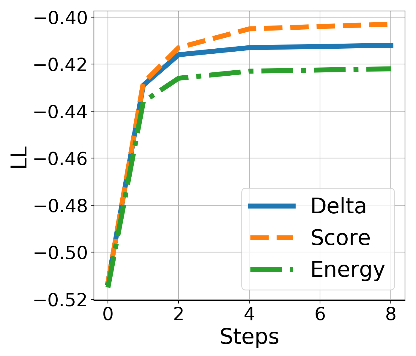
Figure 1: Marginal log probability $\log p_{\theta}(\hat{\bm{\mathrm{y}}}|\bm{\mathrm{x}})$ of output $\hat{\bm{\mathrm{y}}}$ from each refinement step.

Inference speed

We observe that using a learned score function is significantly faster than delta inference: twice as fast on IWSLT’16 De$\rightarrow$En and WMT’16 Ro$\rightarrow$En and almost four times as fast on WMT’14 En$\rightarrow$De. On WMT’14 En$\rightarrow$De, the decoding latency for 4 steps using the score is close to (within one standard deviation of) running 1 refinement step of delta inference. On the other hand, we find that using the learned energy function is slower, presumably due to the overhead from backpropagation. We find its wall clock time to be similar to delta inference. As the entire inference process can be parallelized, we find that parallel decoding with multiple length candidates and latent variable samples only incurs minimal overhead. Finally, we confirm that decoding latency for non-autoregressive models is indeed constant with respect to the sequence length (given parallel computation), as the standard deviation is small ($<10$ ms) across test examples.

Overall result

Overall, we find the proposed inference procedure using the learned score function highly effective and efficient. On WMT’14 En$\rightarrow$De, using 1 refinement step and parallel search leads to $6.2\times$ speedup over the autoregressive baseline with minimal degradation to translation quality (0.9 BLEU score).

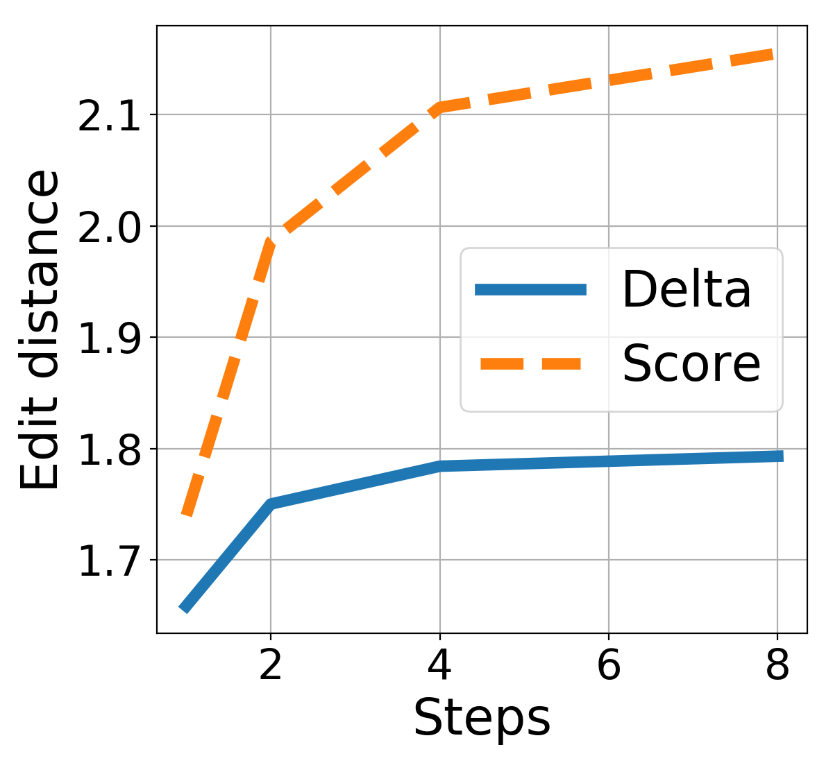
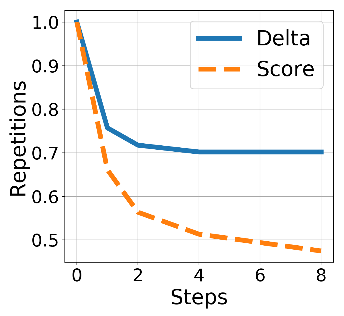
Figure 2: Edit distance from the first output (left) and the number of repetitions in the output (right) for $L=\{1,2,4,8\}$ refinement steps for delta inference and inference using a learned score function.

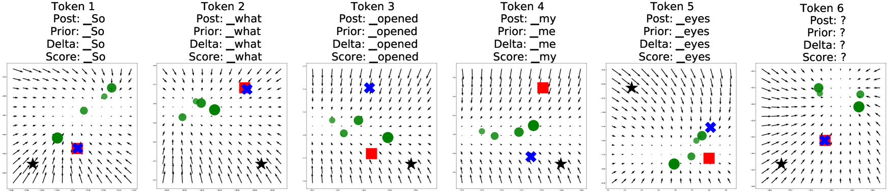
Figure 3: Visualization of estimated gradients and optimization trajectory. Above each plot are tokens predicted from the following latent variables: (1) approximate posterior mean, (2) prior mean, (3) delta inference and (4) inference with the learned score. Black star: latent variable before refinement (prior mean). Blue cross: latent variables after $L=\{1,2,3,4\}$ steps of delta inference (collapsed into a single point). Green circle: latent variables after $L$ steps of inference with a learned score function. Marker size decreases with successive refinement steps. Red square: approximate posterior mean.

5.2 Log Probability Comparison

In Fig 1, we report the marginal log probability $\log p_{\theta}(\hat{\bm{\mathrm{y}}}|\bm{\mathrm{x}})$ of $\hat{\bm{\mathrm{y}}}$ found after $L$ steps of each iterative inference procedure on IWSLT’16 De$\rightarrow$En. We estimate the marginal log probability by importance sampling with 500 samples from the approximate posterior. We observe that the log probability improves with more refinement steps for all inference procedures (delta inference and the proposed procedures). We draw two conclusions from this. First, delta inference indeed increases log probability at each iteration. Second, the proposed optimization scheme increases the target objective function it was trained on (log probability).

5.3 Token Statistics

We compare delta inference and the proposed inference with a learned score function in terms of token statistics in the output translations on IWSLT’16 De$\rightarrow$En. In Figure 2 (left), we compute the average edit distance (in sentencepieces) per test example from the initial output (mean of the prior). It is clear that each refinement step using a learned score function results in more changes in terms of edit distance than delta inference. In Figure 2 (right), we compute the number of token repetitions in the output translations (before removing them in a post-processing step), relative to the initial output. We observe that refining with a learned score function results in less repetitive output compared to delta inference.

6 Qualitative Results

6.1 Visualization of learned gradients

We visualize the learned gradients and the optimization trajectory in Figure 3, from a score inference network trained on a two-dimensional latent variable model on IWSLT’16 De$\rightarrow$En. The example used to generate the visualization is shown below.

Source	Was öffnete mir also die Augen?
Reference	So what opened my eyes ?
Posterior	So what opened my eyes ?
Prior	So what opened me eyes ?
Delta	So what opened me eyes ?
Score	So what opened my eyes ?

We observe that for tokens 1, 2 and 6, delta inference converges quickly to the approximate posterior mean. We also find that the local optima estimated by the score function do not necessarily coincide with the approximate posterior mean. For Token 4, while the local optima estimated by the score function (green circle) is far from the posterior mean (red square), they both map to the reference translation (“my”), indicating that there exist multiple latent variables that map to the reference output.

6.2 Sample translations

We demonstrate that refining in the continuous space results in non-local, non-trivial revisions to the original sentence. For each example in Table 2, we show the English source sentence, German reference sentence, original translation decoded from a sample from the prior, and the revised translation with one gradient update using the estimated score function.

In Example 1, the positions of the main clause (“Es gibt nicht viele Ärzte”) and the prepositional phrase (“im westafrikanischen Land”) are reversed in the continuous refinement process. Inside the main clause, “es gibt” is revised to “gibt es”, a correct grammatical form in German when the prepositional phrase comes before the main clause.

In Example 2, the two numbers are exchanged (“ 1,2 Milliarden Dollar” and “ 6,9 Milliarden Dollar”) in the revised translation. Also, the phrase “aus den” (out of the) is correctly inserted between the two.

In Example 3, the noun phrase “Weisheit in Bedouin” is combined into a single German compound noun “Bedouin-Weisheit”. Also, the phrases “Der erste …” and “mit dieser …” are swapped in the refinement process, to better resemble the reference sentence.

Example 1
Source	There aren ’t many doctors in the west African country ; just one for every 5,000 people
Reference	In dem westafrikanischen Land gibt es nicht viele Ärzte, nur einen für 5.000 Menschen
Original	Es gibt nicht viele Ärzte im westafrikanischen Land, nur eine für 5.000 Menschen.
Refined	Im westafrikanischen Land gibt es nicht viele Ärzte, nur eine für 5.000 Menschen.
Example 2
Source	Costumes are expected to account for $ 1.2 billion dollars out of the $ 6.9 billion spent , according to the NRF .
Reference	Die Kostüme werden etwa 1,2 Milliarden der 6,9 Milliarden ausgegebenen US-Dollar ausmachen, so der NRF.
Original	Es wird von, Kostüme, dass sie die dem NRF ausgegebenen 6,9 Milliarden Dollar 1,2 Milliarden Dollar
	ausmachen.
Refined	Es wird erwartet, dass die Kostüme nach Angaben des NRF 1,2 Milliarden Dollar aus den 6,9 Milliarden Dollar
	ausmachen.
Example 3
Source	It was with this piece of Bedouin wisdom that the first ever chairman Wolfgang Henne described the history and
	fascination behind the “Helping Hands” society .
Reference	Mit dieser Beduinenweisheit beschrieb der erste Vorsitzende Wolfgang Henne die Geschichte und Faszination des
	Vereins “Helfende Hände”.
Original	Der erste Vorsitzende Wolfgang Henne beschrieb mit dieser erste Weisheit in Bedouin” die Geschichte und
	Faszination hinter der “Helenden Hands” Gesellschaft
Refined	Mit diesem Stück Bedouin-Weisheit beschrieb der erste Vorsitzende Wolfgang Henne jemals die Geschichte und
	Faszination hinter der “Heling Hands” Gesellschaft

Table 2: Sample translations on WMT’14 En$\rightarrow$De. We show the translation from a latent variable sampled from the prior (Original) and the translation after one refinement step in the continuous space with the learned score function (Refined). We emphasize phrases whose positions are swapped in the refinement process in red and blue.

7 Related Work

Learning

Our training objective is closely related to the score matching objective Hyvärinen (2005), with the following differences. First, we approximate the gradient of the data log density using a proxy gradient, whereas this term is replaced by the Hessian of the energy in the original score matching objective. Second, we only consider samples from the prior. Saremi et al. (2018) proposed a denoising interpretation of the Parzen score objective (Vincent, 2011) that avoids estimating the Hessian. Although score function estimation that bypasses energy estimation was found to be unstable (Alain and Bengio, 2014; Saremi et al., 2018), it has been successfully applied to generative modeling of images (Song and Ermon, 2019).

Inference

While we categorize inference methods for machine translation as (1) discrete search, (2) hybrid optimization (Shu et al., 2020) and (3) continuous optimization (this work) in Section 2, another line of work relaxes discrete search into continuous optimization (Hoang et al., 2017; Gu et al., 2018b; Tu et al., 2020). By using Gumbel-softmax relaxation (Maddison et al., 2017; Jang et al., 2017), they train an inference network to generate target tokens that maximize the log probability under a pretrained model.

Gradient-based Inference

Performing gradient descent over structured outputs was mentioned in  LeCun et al. (2006), and has been successfully applied to many structured prediction tasks (Belanger and McCallum, 2016; Wang et al., 2016; Belanger et al., 2017). Other work performed gradient descent over the latent variables to optimize objectives for a wide variety of tasks, including chemical design (Gómez-Bombarelli et al., 2018) and text generation (Mueller et al., 2017)

Generation by Refinement

Refinement has a long history in text generation. The retrieve-and-refine framework retrieves an (input, output) pair from the training set that is similar to the test example, and performs edit operations on the corresponding output (Sumita and Iida, 1991; Song et al., 2016; Hashimoto et al., 2018; Weston et al., 2018; Gu et al., 2018c). The idea of refinement has also been applied in automatic post-editing (Novak et al., 2016; Grangier and Auli, 2017).

8 Conclusion

We propose an efficient inference procedure for non-autoregressive machine translation that refines translations purely in the continuous space. Given a latent variable model for machine translation, we train an inference network to approximate the gradient of the marginal log probability with respect to the target sentence, using only the latent variable. This allows us to use gradient based optimization to find a target sentence at inference time that approximately maximizes the marginal log probability. As we avoid discrete search over a large vocabulary, our inference procedure is more efficient than previous inference procedures that refine in the token space.

We compare our approach with a recently proposed delta inference procedure that optimizes jointly in discrete and continuous space on three machine translation datasets: WMT’14 En$\rightarrow$De, WMT’16 Ro$\rightarrow$En and IWSLT’16 De$\rightarrow$En. With the same underlying latent variable model, the proposed inference procedure using a learned score function has following advantages: (1) it is twice as fast as delta inference, and (2) it is able to find target sentences resulting in higher marginal probabilities and BLEU scores.

While we showed that iterative inference with a learned score function is effective for spherical Gaussian priors, more work is required to investigate if such an approach will also be successful for more sophisticated priors, such as Gaussian mixtures or normalizing flows. This will be particularly interesting, as recent study showed latent variable models with a flexible prior give high test log-likelihoods, but suffer from poor generation quality as inference is challenging (Lee et al., 2020).

Appendix A Training objective

$$\min_{\psi}\> \Big{\|}\Big{(}-E_{\psi}(\overline{\bm{\mathrm{z}}})+E_{\psi}(\bm{\mathrm{z}})\Big{)}-\Big{(}\tau(\overline{\bm{\mathrm{z}}})-\tau(\bm{\mathrm{z}})\Big{)}\Big{\|}^{2}$$

$$\approx\min_{\psi}\> \Big{\|}\Big{(}(\overline{\bm{\mathrm{z}}}-\bm{\mathrm{z}})^{\intercal}\cdot\nabla_{\bm{\mathrm{z}}}(-E_{\psi}(\bm{\mathrm{z}}))\Big{)}$$

$$-\Big{(}(\overline{\bm{\mathrm{z}}}-\bm{\mathrm{z}})^{\intercal}\cdot\nabla_{\bm{\mathrm{z}}}\tau(\bm{\mathrm{z}})\Big{)}\Big{\|}^{2}$$ (5)

$$\approx\min_{\psi}\> \Big{\|}\big{(}\overline{\bm{\mathrm{z}}}-\bm{\mathrm{z}}\big{)}^{\intercal}\Big{(}\nabla_{\bm{\mathrm{z}}}(-E_{\psi}(\bm{\mathrm{z}}))-\nabla_{\bm{\mathrm{z}}}\tau(\bm{\mathrm{z}})\Big{)}\Big{\|}^{2}$$

$$\approx\min_{\psi}\> \Big{(}\nabla_{\bm{\mathrm{z}}}(-E_{\psi}(\bm{\mathrm{z}}))-\nabla_{\bm{\mathrm{z}}}\tau(\bm{\mathrm{z}})\Big{)}^{\intercal}\big{(}\overline{\bm{\mathrm{z}}}-\bm{\mathrm{z}}\big{)}$$

$$\big{(}\overline{\bm{\mathrm{z}}}-\bm{\mathrm{z}}\big{)}^{\intercal}\Big{(}\nabla_{\bm{\mathrm{z}}}(-E_{\psi}(\bm{\mathrm{z}}))-\nabla_{\bm{\mathrm{z}}}\tau(\bm{\mathrm{z}})\Big{)}$$

$$\approx\min_{\psi}\> \Big{(}\nabla_{\bm{\mathrm{z}}}(-E_{\psi}(\bm{\mathrm{z}}))-\nabla_{\bm{\mathrm{z}}}\tau(\bm{\mathrm{z}})\Big{)}^{\intercal}\big{\|}\overline{\bm{\mathrm{z}}}-\bm{\mathrm{z}}\big{\|}^{2}$$

$$\Big{(}\nabla_{\bm{\mathrm{z}}}(-E_{\psi}(\bm{\mathrm{z}}))-\nabla_{\bm{\mathrm{z}}}\tau(\bm{\mathrm{z}})\Big{)}$$ (6)

$$\approx\min_{\psi}\> \Big{\|}\nabla_{\bm{\mathrm{z}}}(-E_{\psi}(\bm{\mathrm{z}}))-\nabla_{\bm{\mathrm{z}}}\tau(\bm{\mathrm{z}})\Big{\|}^{2}$$

$$\approx\min_{\psi}\> \Big{\|}\nabla_{\bm{\mathrm{z}}}(-E_{\psi}(\bm{\mathrm{z}}))\Big{\|}^{2}+\Big{\|}\nabla_{\bm{\mathrm{z}}}\tau(\bm{\mathrm{z}})\Big{\|}^{2}$$

$$-2\,\Big{(}\nabla_{\bm{\mathrm{z}}}(-E_{\psi}(\bm{\mathrm{z}}))^{\intercal}\cdot\nabla_{\bm{\mathrm{z}}}\tau(\bm{\mathrm{z}})\Big{)}$$ (7)

$$\approx\min_{\psi}\> \Big{\|}\nabla_{\bm{\mathrm{z}}}E_{\psi}(\bm{\mathrm{z}})\Big{\|}^{2}+2\,\Big{(}\nabla_{\bm{\mathrm{z}}}E_{\psi}(\bm{\mathrm{z}})^{\intercal}\cdot\nabla_{\bm{\mathrm{z}}}\tau(\bm{\mathrm{z}})\Big{)}$$

Eq. 5 follows from linear approximation, as

$$-\big{(}E_{\psi}(\overline{\bm{\mathrm{z}}})-E_{\psi}(\bm{\mathrm{z}})\big{)} \approx(\overline{\bm{\mathrm{z}}}-\bm{\mathrm{z}})^{\intercal}\cdot\nabla_{\bm{\mathrm{z}}}(-E_{\psi}(\bm{\mathrm{z}}))$$

$$\tau(\overline{\bm{\mathrm{z}}})-\tau(\bm{\mathrm{z}}) \approx(\overline{\bm{\mathrm{z}}}-\bm{\mathrm{z}})^{\intercal}\cdot\nabla_{\bm{\mathrm{z}}}\tau(\bm{\mathrm{z}})$$

$\|\overline{\bm{\mathrm{z}}}-\bm{\mathrm{z}}\|^{2}$ in Eq. 6 can be eliminated, as dividing the objective with a positive constant does not change the solution. The second term in Eq. 7 is also a constant with respect to $\psi$, hence can be ignored.

References

- Alain and Bengio (2014) Guillaume Alain and Yoshua Bengio. 2014. What regularized auto-encoders learn from the data-generating distribution. J. Mach. Learn. Res., 15(1):3563–3593.
- Belanger and McCallum (2016) David Belanger and Andrew McCallum. 2016. Structured prediction energy networks. In Proceedings of the 33nd International Conference on Machine Learning, volume 48 of JMLR Workshop and Conference Proceedings, pages 983–992.
- Belanger et al. (2017) David Belanger, Bishan Yang, and Andrew McCallum. 2017. End-to-end learning for structured prediction energy networks. In Proceedings of the 34th International Conference on Machine Learning, volume 70 of Proceedings of Machine Learning Research, pages 429–439. PMLR.
- Chan et al. (2019) William Chan, Nikita Kitaev, Kelvin Guu, Mitchell Stern, and Jakob Uszkoreit. 2019. KERMIT: generative insertion-based modeling for sequences. arXiv preprint arxiv:1906.01604.
- Ghazvininejad et al. (2019) Marjan Ghazvininejad, Omer Levy, Yinhan Liu, and Luke Zettlemoyer. 2019. Mask-predict: Parallel decoding of conditional masked language models. In Proceedings of the 2019 Conference on Empirical Methods in Natural Language Processing and the 9th International Joint Conference on Natural Language Processing, EMNLP-IJCNLP, pages 6111–6120.
- Gómez-Bombarelli et al. (2018) Rafael Gómez-Bombarelli, Jennifer N. Wei, David Duvenaud, José Miguel Hernández-Lobato, Benjamín Sánchez-Lengeling, Dennis Sheberla, Jorge Aguilera-Iparraguirre, Timothy D. Hirzel, Ryan P. Adams, and Alán Aspuru-Guzik. 2018. Automatic chemical design using a data-driven continuous representation of molecules. ACS Central Science, 4(2):268–276.
- Grangier and Auli (2017) David Grangier and Michael Auli. 2017. Quickedit: Editing text & translations via simple delete actions. arXiv preprint arXiv:1711.04805.
- Gu et al. (2018a) Jiatao Gu, James Bradbury, Caiming Xiong, Victor O. K. Li, and Richard Socher. 2018a. Non-autoregressive neural machine translation. In 6th International Conference on Learning Representations, ICLR.
- Gu et al. (2018b) Jiatao Gu, Daniel Jiwoong Im, and Victor O. K. Li. 2018b. Neural machine translation with gumbel-greedy decoding. In Proceedings of the Thirty-Second AAAI Conference on Artificial Intelligence, pages 5125–5132. AAAI Press.
- Gu et al. (2019) Jiatao Gu, Qi Liu, and Kyunghyun Cho. 2019. Insertion-based decoding with automatically inferred generation order. Trans. Assoc. Comput. Linguistics, 7:661–676.
- Gu et al. (2018c) Jiatao Gu, Yong Wang, Kyunghyun Cho, and Victor O. K. Li. 2018c. Search engine guided neural machine translation. In Proceedings of the Thirty-Second AAAI Conference on Artificial Intelligence, pages 5133–5140. AAAI Press.
- Hashimoto et al. (2018) T. Hashimoto, K. Guu, Y. Oren, and P. Liang. 2018. A retrieve-and-edit framework for predicting structured outputs. In Advances in Neural Information Processing Systems (NeurIPS).
- Hoang et al. (2017) Cong Duy Vu Hoang, Gholamreza Haffari, and Trevor Cohn. 2017. Towards decoding as continuous optimisation in neural machine translation. In Proceedings of the 2017 Conference on Empirical Methods in Natural Language Processing, pages 146–156. Association for Computational Linguistics.
- Hyvärinen (2005) Aapo Hyvärinen. 2005. Estimation of non-normalized statistical models by score matching. J. Mach. Learn. Res., 6:695–709.
- Jang et al. (2017) Eric Jang, Shixiang Gu, and Ben Poole. 2017. Categorical reparameterization with gumbel-softmax. In 5th International Conference on Learning Representations. OpenReview.net.
- Kaiser et al. (2018) Lukasz Kaiser, Samy Bengio, Aurko Roy, Ashish Vaswani, Niki Parmar, Jakob Uszkoreit, and Noam Shazeer. 2018. Fast decoding in sequence models using discrete latent variables. In Proceedings of the 35th International Conference on Machine Learning, ICML, pages 2395–2404.
- Kim and Rush (2016) Yoon Kim and Alexander M. Rush. 2016. Sequence-level knowledge distillation. In Proceedings of the 2016 Conference on Empirical Methods in Natural Language Processing, EMNLP, pages 1317–1327.
- Kingma and Ba (2015) Diederik P. Kingma and Jimmy Ba. 2015. Adam: A method for stochastic optimization. In 3rd International Conference on Learning Representations, ICLR.
- Kingma and Welling (2014) Diederik P. Kingma and Max Welling. 2014. Auto-encoding variational bayes. In 2nd International Conference on Learning Representations, ICLR 2014, Banff, AB, Canada, April 14-16, 2014, Conference Track Proceedings.
- Kudo and Richardson (2018) Taku Kudo and John Richardson. 2018. Sentencepiece: A simple and language independent subword tokenizer and detokenizer for neural text processing. In Proceedings of the 2018 Conference on Empirical Methods in Natural Language Processing, pages 66–71. Association for Computational Linguistics.
- LeCun et al. (2006) Yann LeCun, Sumit Chopra, Raia Hadsell, Fu Jie Huang, and et al. 2006. A tutorial on energy-based learning. In Predicting Structured Data. MIT Press.
- Lee et al. (2018) Jason Lee, Elman Mansimov, and Kyunghyun Cho. 2018. Deterministic non-autoregressive neural sequence modeling by iterative refinement. In Proceedings of the 2018 Conference on Empirical Methods in Natural Language Processing, pages 1173–1182.
- Lee et al. (2020) Jason Lee, Dustin Tran, Orhan Firat, and Kyunghyun Cho. 2020. On the discrepancy between density estimation and sequence generation. arXiv preprint arxiv:2002.07233.
- Ma et al. (2019) Xuezhe Ma, Chunting Zhou, Xian Li, Graham Neubig, and Eduard H. Hovy. 2019. Flowseq: Non-autoregressive conditional sequence generation with generative flow. In Proceedings of the 2019 Conference on Empirical Methods in Natural Language Processing, pages 4281–4291.
- Maddison et al. (2017) Chris J. Maddison, Andriy Mnih, and Yee Whye Teh. 2017. The concrete distribution: A continuous relaxation of discrete random variables. In 5th International Conference on Learning Representations.
- Mansimov et al. (2019) Elman Mansimov, Alex Wang, and Kyunghyun Cho. 2019. A generalized framework of sequence generation with application to undirected sequence models. arXiv preprint arxiv:1905.12790.
- Mueller et al. (2017) Jonas Mueller, David K. Gifford, and Tommi S. Jaakkola. 2017. Sequence to better sequence: Continuous revision of combinatorial structures. In Proceedings of the 34th International Conference on Machine Learning, volume 70 of Proceedings of Machine Learning Research, pages 2536–2544. PMLR.
- Novak et al. (2016) Roman Novak, Michael Auli, and David Grangier. 2016. Iterative refinement for machine translation. arXiv preprint arXiv:1610.06602.
- Ott et al. (2019) Myle Ott, Sergey Edunov, Alexei Baevski, Angela Fan, Sam Gross, Nathan Ng, David Grangier, and Michael Auli. 2019. fairseq: A fast, extensible toolkit for sequence modeling. In Proceedings of the 2019 Conference of the North American Chapter of the Association for Computational Linguistics: Human Language Technologies, pages 48–53. Association for Computational Linguistics.
- Post (2018) Matt Post. 2018. A call for clarity in reporting BLEU scores. In Proceedings of the Third Conference on Machine Translation: Research Papers, pages 186–191. Association for Computational Linguistics.
- Saremi et al. (2018) Saeed Saremi, Arash Mehrjou, Bernhard Schölkopf, and Aapo Hyvärinen. 2018. Deep energy estimator networks. arXiv preprint arxiv:1805.08306.
- Sennrich et al. (2016) Rico Sennrich, Barry Haddow, and Alexandra Birch. 2016. Edinburgh neural machine translation systems for WMT 16. In Proceedings of the First Conference on Machine Translation, WMT, pages 371–376.
- Shu et al. (2020) Raphael Shu, Jason Lee, Hideki Nakayama, and Kyunghyun Cho. 2020. Latent-variable non-autoregressive neural machine translation with deterministic inference using a delta posterior. In Proceedings of the Thirty-Fourth AAAI Conference on Artificial Intelligence.
- Song and Ermon (2019) Yang Song and Stefano Ermon. 2019. Generative modeling by estimating gradients of the data distribution. In Advances in Neural Information Processing Systems 32: Annual Conference on Neural Information Processing Systems 2019, pages 11895–11907.
- Song et al. (2016) Yiping Song, Rui Yan, Xiang Li, Dongyan Zhao, and Ming Zhang. 2016. Two are better than one: An ensemble of retrieval- and generation-based dialog systems. arXiv preprint arxiv:1610.07149.
- Sumita and Iida (1991) Eiichiro Sumita and Hitoshi Iida. 1991. Experiments and prospects of example-based machine translation. In 29th Annual Meeting of the Association for Computational Linguistics, pages 185–192. Association for Computational Linguistics.
- Teh et al. (2003) Yee Whye Teh, Max Welling, Simon Osindero, and Geoffrey E. Hinton. 2003. Energy-based models for sparse overcomplete representations. J. Mach. Learn. Res., 4:1235–1260.
- Tu et al. (2020) Lifu Tu, Richard Yuanzhe Pang, Sam Wiseman, and Kevin Gimpel. 2020. Engine: Energy-based inference networks for non-autoregressive machine translation.
- Vaswani et al. (2017) Ashish Vaswani, Noam Shazeer, Niki Parmar, Jakob Uszkoreit, Llion Jones, Aidan N. Gomez, Lukasz Kaiser, and Illia Polosukhin. 2017. Attention is all you need. In Advances in Neural Information Processing Systems 30: Annual Conference on Neural Information Processing Systems, pages 5998–6008.
- Vincent (2011) Pascal Vincent. 2011. A connection between score matching and denoising autoencoders. Neural Computation, 23(7):1661–1674.
- Wainwright and Jordan (2008) Martin J. Wainwright and Michael I. Jordan. 2008. Graphical models, exponential families, and variational inference. Foundations and Trends in Machine Learning, 1(1-2):1–305.
- Wang et al. (2016) Shenlong Wang, Sanja Fidler, and Raquel Urtasun. 2016. Proximal deep structured models. In Advances in Neural Information Processing Systems 29: Annual Conference on Neural Information Processing Systems, pages 865–873.
- Weston et al. (2018) Jason Weston, Emily Dinan, and Alexander H. Miller. 2018. Retrieve and refine: Improved sequence generation models for dialogue. In Proceedings of the 2nd International Workshop on Search-Oriented Conversational AI, SCAI@EMNLP 2018, Brussels, Belgium, October 31, 2018, pages 87–92. Association for Computational Linguistics.