Gaining or Losing Perspective for
Piecewise-Linear Under-Estimators of
Convex Univariate Functions

Abstract

We study MINLO (mixed-integer nonlinear optimization) formulations of the disjunction $x\in\{0\}\cup[\ell,u]$, where $z$ is a binary indicator of $x\in[\ell,u]$ ($0\leq\ell<u$), and $y$ “captures” $f(x)$, which is assumed to be convex and positive on its domain $[\ell,u]$, but otherwise $y=0$ when $x=0$. This model is very useful in nonlinear combinatorial optimization, where there is a fixed cost of operating an activity at level $x$ in the operating range $[\ell,u]$, and then there is a further (convex) variable cost $f(x)$. In particular, we study relaxations related to the perspective transformation of a natural piecewise-linear under-estimator of $f$, obtained by choosing linearization points for $f$. Using 3-d volume (in $(x,y,z)$) as a measure of the tightness of a convex relaxation, we investigate relaxation quality as a function of $f$, $\ell$, $u$, and the linearization points chosen. We make a detailed investigation for convex power functions $f(x):=x^{p}$, $p>1$.

1 Introduction

1.1 Definitions and background

Let $f$ be a univariate convex function with domain $[\ell,u]$, where $0\leq\ell<u$. We assume that $f$ is positive on $[\ell,u]$. We are interested in the mathematical-optimization context of modeling a function, represented by a variable $y$, that is equal to a given convex function $f(x)$ on an “operating range” $[\ell,u]$ and equal to $0$ at $0$. We do this using a $0/1$ indicator variable $z$ (which conveniently allows for incorporating a fixed cost for $x$ being in the operating range), and we represent the relevant set disjunctively as follows. We define

$$\invbreve{D}_{f}(\ell,u):= \{(0,0,0)\}{\textstyle\bigcup}\left\{(x,y,1)\in\mathbb{R}^{3}~{}\negthinspace\negthinspace:~{}\negthinspace\negthinspace\negthinspace\negthinspace\vphantom{\scriptstyle\frac{f(u)-f(\ell)}{u-\ell}}\right.\left.f(\ell)+{\scriptstyle\frac{f(u)-f(\ell)}{u-\ell}}(x-\ell)\geq y\geq f(x),~{}u\geq x\geq\ell\right\}.$$

Notice that for $x\in\{\ell,u\}$, we have $y=f(x)$. So, the upper bound on $y$ enables us to capture the convex hull of the graph of the convex $f(x)$ on $[\ell,u]$, in the $z=1$ plane.

Next, following the notation of Perspec2019 , we define the perspective relaxation

$$\invbreve{S}^{*}_{f}(\ell,u):=\operatorname{convcl}\left\{(x,y,z)\in\mathbb{R}^{3}~{}:~{}\left(f(\ell)-{\scriptstyle\frac{f(u)-f(\ell)}{u-\ell}}\ell\right)z+{\scriptstyle\frac{f(u)-f(\ell)}{u-\ell}}x\geq y\geq zf(x/z),~{}\right.$$

$$\left.uz\geq x\geq\ell z,~{}1\geq z>0,~{}y\geq 0\vphantom{\scriptstyle\frac{f(u)-f(\ell)}{u-\ell}}\right\},$$

where $\operatorname{convcl}$ denotes the convex closure operator. Notice that “perspectivizing” the convex $f(x)$ produces a more complicated but still convex function $zf(x/z)$, and handling such a function pushes us into the realm of conic programming. On the other side, perspectivizing the (univariate) linear upper bound on $y$ leads to a (bivariate but still) linear upper bound on $y$. Intersecting $\invbreve{S}^{*}_{f}(\ell,u)$ with the hyperplane defined by $z=0$, leaves the single point $(x,y,z)=(0,0,0)$, which is only in the set after we take the closure. In this way, the “perspective and convex closure” construction gives us exactly the value $y=0$ that we want at $x=0$. Moreover, $\invbreve{S}^{*}_{f}(\ell,u)$ is precisely the convex closure of $\invbreve{D}_{f}(\ell,u)$.

We compare convex bodies relaxing $\invbreve{S}^{*}_{f}(\ell,u)$ via their volumes, with an eye toward weighing the relative tightness of relaxations against the difficulty of solving them. Generally, working with $\invbreve{S}^{*}_{f}(\ell,u)$ implies using a cone solver (e.g., Mosek), while relaxations imply the possibility of using more general NLP or even LP solvers; see Perspec2019 for more discussion on this important motivating subject. One key relaxation previously studied requires that the domain of $f$ is all of $[0,u]$, $f$ is convex on $[0,u]$, $f(0)=0$, and $f$ is increasing on $[0,u]$. For example, convex power functions $f(x):=x^{p}$ with $p>1$ have these properties. Assuming these properties, we define the naïve relaxation

$$\invbreve{S}^{0}_{f}(\ell,u):=\left\{(x,y,z)\in\mathbb{R}^{3}~{}:~{}\left(f(\ell)-{\scriptstyle\frac{f(u)-f(\ell)}{u-\ell}}\ell\right)z+{\scriptstyle\frac{f(u)-f(\ell)}{u-\ell}}x\geq y\geq f(x),~{}\right.$$

$$\left.uz\geq x\geq\ell z,~{}1\geq z\geq 0\vphantom{\scriptstyle\frac{f(u)-f(\ell)}{u-\ell}}\right\}.$$

While the naïve relaxation is weaker than the perspective relaxation, it can be handled more efficiently and by a wider class of solvers because of its simpler form involving $f(x)$ rather than $zf(x/z)$.

1.2 Relation to previous literature

The perspective transformation of a convex function is well known in mathematics (see perspecbook , for example). Applying it in the context of our disjunction is also well studied (see gunlind1 ; Frangioni2006 ; Akturk , with applications to nonlinear facility location and also mean-variance portfolio optimization in the style of Markowitz). The idea of using volume to compare relaxations was introduced by LM1994 (also see LeeSkipperSpeakmanMPB2018 and the references therein). Recently, PerspectiveWCGO ; Perspec2019 applied the idea of using volumes to evaluate and compare the perspective relaxation with other relaxations of our disjunction.

Piecewise linearization is a very well studied and useful concept for handling nonlinearities (see, for example, CharnesLemke ; LeeWilson and also the more recent Viel ; TorViel and the many references therein). It is a natural idea to strengthen a convex piecewise linearization of a convex univariate function using the perspective idea, and then to evaluate it using volume computation. This is what we pursue here, concentrating on piecewise-linear under-estimators of univariate convex functions. We also wish to mention and emphasize that our techniques are directly relevant for (additively) separable convex functions (see Bonami ; Berenguel , and of course all of the exact global-optimization solvers (which induce a lot of separability via reformulation using additional variables).

1.3 Our contribution and organization

Our focus is on relaxations related to natural piecewise-linear under-estimators of $f$. Piecewise linearization is a standard method for efficiently handling nonlinearities in optimization. For a convex function, it is easy to get a piecewise-linear under-estimator. But there are a few issues to consider: the number of linearization points, how to choose them, and how to handle the resulting piecewise-linearization.

In particular, we look at the behavior of the perspective relaxation associated with a natural piecewise-linear under-estimator of a convex univariate function, as we vary the placement and the number of linearization points describing the piecewise-linear under-estimator.

In §2, we introduce notation for a natural piecewise-linear under-estimator $g$ of $f$ on $[\ell,u]$, using linearizations of $f(x)$ at $n+1(\geq 2)$ values of $x$, namely $\ell=:\xi_{0}<\xi_{1}<\cdots<\xi_{n}:=u$, we define the convex relaxation $\invbreve{U}^{*}_{f}(\bm{\xi}):=\invbreve{S}^{*}_{g}(\ell,u)$, and we describe an efficient algorithm for determining its volume (Theorem 2.1 and Corollary 2). Armed with this efficient algorithm, any global-optimization software could decide between members of this family of formulations (depending on the number and placement of linearization points) and also alternatives (e.g., $\invbreve{S}^{*}_{f}(\ell,u)$ and $\invbreve{S}^{0}_{f}(\ell,u)$, explored in Perspec2019 ), trading off tightness of the formulations against the relative ease/difficulty of working with them computationally.

In §3, we give a more detailed analysis for convex power functions $f(x):=x^{p}$, for $p>1$. In §3.1, focusing on quadratics ($p=2$), we solve the volume-minimization problem for $\operatorname{vol}(\invbreve{U}^{*}_{f}(\bm{\xi}))$ when $p=2$ (Theorem 3.1), for an arbitrary number of linearization points, thus finding the optimal placement of linearization points for convex quadratics. Further, from this, we recover the associated formula from Perspec2019 for $\operatorname{vol}(\invbreve{S}^{*}_{f}(\ell,u))$ (Corollary 2), and we demonstrate that the minimum volume is always less than the volume of the naïve relaxation when $p=2$ (Corollary 3). In §3.2, focusing on non-quadratics ($p\not=2$), we first demonstrate with Theorem 3.4 that all stationary points are strict local minimizer. Next, with Theorem 3.5, we demonstrate that for $p\leq 2$, that the volume function is strictly convex, and so in this case (Corollary 6), we can conclude that it has a unique minimizer. We establish that this also holds for $p>2$ (Theorem 3.9 and Corollary 10). We also establish that the optimal location of each linearization point is increasing in $p$ on $(1,\infty)$ (Theorem 3.11). Finally, we establish a nice monotone behavior for Newton’s method on our volume minimization problem (Theorem 3.13). In §3.3, we consider optimal placement of a single non-boundary linearization point. Furthermore, via a simple transformation, for the tricky case of minimizing $\operatorname{vol}(\invbreve{U}^{*}_{p}(\ell,\xi_{1},u))$ when $p>2$, we can reduce that problem to maximizing a strictly concave function (Theorem 3.17). Next, we provide some bounds on the minimizing $\xi_{1}$ (Theorem 3.18). This can be useful on determining a reasonable initial point for a minimization algorithm or even for a reasonable static rule for selecting linearization points. Next, we establish how good our bounds are in the case of $\ell=0$ (Proposition 20).

In §4, we consider several related relaxations that are less computational burdensome than the perspective relaxation applied to a convex power function or even to a piecewise-linear under-estimator. To demonstrate the type of results that can be established, we focus on convex power functions and ultimately quadratics with equally-spaced linearization points. In particular, we establish how many linearization points are needed for various approximations.

2 Piecewise-linear under-estimation and perspective

Piecewise-linear estimation is widely used in optimization. LeeWilson provides some key relaxations using integer variables, even for non-convex functions on multidimensional (polyhedral) domains. We are particularly interested in piecewise-linear under-estimation because of its value in global optimization.

Given convex $f:[\ell,u]\rightarrow\mathbb{R}_{++}$, we consider linearization points

$$\ell=:\xi_{0}<\xi_{1}<\cdots<\xi_{n}:=u$$

in the domain of $f$, and we assume that $f$ is differentiable at these $\xi_{i}$.

At each $\xi_{i}$, we have the tangent line

$$y=f(\xi_{i})+f^{\prime}(\xi_{i})(x-\xi_{i}), T_{i}$$ ()

for $i=0,\ldots,n$. Considering tangent lines $T_{i}$ and $T_{i-1}$ (for adjacent points), we have the intersection point

$$(x,y):=(\tau_{i},~{}f(\xi_{i})+f^{\prime}(\xi_{i})(\tau_{i}-\xi_{i})),\hbox{ for $i=1,\ldots,n$}, P_{i}$$ ()

where

$$\tau_{i}:=\frac{\left[f(\xi_{i})-f^{\prime}(\xi_{i})\xi_{i}\right]-\left[f(\xi_{i-1})-f^{\prime}(\xi_{i-1})\xi_{i-1}\right]}{f^{\prime}(\xi_{i-1})-f^{\prime}(\xi_{i})}.$$

Finally, we define

$$(x,y):=(\tau_{0}:=\ell,f(\ell)) P_{0}$$ ()

and

$$(x,y):=(\tau_{n+1}:=u,f(u)). P_{n+1}$$ ()

It is easy to see that $\ell=:\tau_{0}<\tau_{1}<\cdots<\tau_{n+1}:=u,$ and that the piecewise-linear function $g:[\ell,u]\rightarrow\mathbb{R}$, defined as the function having the graph that connects the $P_{i}$, for $i=0,1,\ldots,n+1$, is a convex under-estimator of $f$ (agreeing with $f$ at the $\xi_{i}$; see Fig. 1. In what follows, $g$ is always defined as above (from $f$ and $\bm{\xi}$).

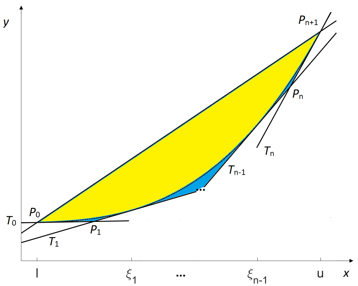
Figure 1: Piecewise-linear under-estimator

We wish to compute the volume of the set $\invbreve{U}^{*}_{f}(\bm{\xi}):=\invbreve{S}^{*}_{g}(\ell,u)$. To proceed, we work with the sequence $\tau_{0},\tau_{1},\ldots,\tau_{n+1}$ defined above. Below and later, $\operatorname{adet}$ denotes the absolute value of the determinant.

Theorem 2.1.

$$\operatorname{vol}(\invbreve{U}^{*}_{f}(\bm{\xi}))=\frac{1}{6}\sum_{i=1}^{n}\operatorname{adet}\left(\begin{array}[]{ccc}\tau_{0}&\tau_{i}&\tau_{i+1}\\ g(\tau_{0})&g(\tau_{i})&g(\tau_{i+1})\\ 1&1&1\end{array}\right).$$

Proof.

We wish to compute the volume of the set $\invbreve{U}^{*}_{f}(\bm{\xi})$. This set is a pyramid with apex $(x,y,z)=(0,0,0)$ and base equal to the intersection of $\invbreve{U}^{*}_{f}(\bm{\xi})$ with the hyperplane defined by the equation $z=1$. The height of the apex over the base is unity. So the volume of $\invbreve{U}^{*}_{f}(\bm{\xi})$ is simply the area of the base divided by 3. We will compute the area of the base by straightforward 2-d triangulation. Our triangles are $\operatorname{conv}\{P_{0},P_{i},P_{i+1}\}$, for $i=1,\ldots,n$. The area of each triangle is $1/2$ of the absolute determinant of an appropriate $3\times 3$ matrix. The formula follows. ∎

Corollary 2.

Assuming oracle access to $f$ and $f^{\prime}$, we can compute $\operatorname{vol}(\invbreve{U}^{*}_{f}(\bm{\xi}))$ in $\mathcal{O}(n)$ time.

3 Analysis of convex power functions

Convex power functions constitute a broad and flexible class of increasing convex univariate functions, useful in a wide variety of applications. Additionally, an ability to handle the power functions $x^{k}$ for integers $k\geq 2$, already gives us a lower-bounding method for $f(x):=\exp(x)$ by truncating its Maclaurin series $\sum_{k=1}^{\infty}x^{k}/k!$, and working termwise (on the terms $k\geq 2$). More generally, we could approach any univariate function $f:\mathbb{R}\rightarrow\mathbb{R}_{+}$ like this, as long as its Maclaurin series has all nonnegative coefficients; i.e., when all derivatives at $0$ are nonnegative. For example, $1/(1-x)^{k}$ with integer $k\geq 1$ (i.e., the geometric series and its derivatives), $\sinh(x)$ and $\tan(x)$ for $x<\pi/2$, and $\arcsin(x)$ for $x<1$. Therefore, analyzing relaxations for power functions, can have rather broad applicability.

For convenience, let $\invbreve{U}^{*}_{p}(\bm{\xi})$ denote $\invbreve{U}^{*}_{f}(\bm{\xi})$, with $f(x):=x^{p}$, $p>1$.

3.1 Quadratics

We will see that equally-spaced linearization points minimizes the volume of the relaxation $\invbreve{U}^{*}_{p}(\bm{\xi})$ when $p=2$.

Theorem 3.1.

Given $n\geq 2$, $0\leq\xi_{0}:=\ell<\xi_{1}<\dots<\xi_{n-1}<u=:\xi_{n}$, we have that $\xi_{i}:=\ell+\frac{i}{n}(u-\ell)$, for $i=1,\ldots,n-1$, is the unique minimizer of $\operatorname{vol}(\invbreve{U}^{*}_{2}(\bm{\xi}))$, and the minimum volume is $\frac{1}{18}(u-\ell)^{3}+\frac{(u-\ell)^{3}}{36n^{2}}$.

Proof.

The intersection points $P_{i}$ are $(\frac{\xi_{i-1}+\xi_{i}}{2},\xi_{i-1}\xi_{i})$. We have $\tau_{i}=\frac{\xi_{i-1}+\xi_{i}}{2}$ for $i=1,\ldots,n+1$, and

$$\operatorname{vol}(\invbreve{U}^{*}_{2}(\bm{\xi})) =\frac{1}{6}\sum_{i=1}^{n}\operatorname{adet}\begin{pmatrix}\tau_{0}&\tau_{i}&\tau_{i+1}\\ g(\tau_{0})&g(\tau_{i})&g(\tau_{i+1})\\ 1&1&1\end{pmatrix}$$

$$=\frac{1}{12}\sum_{i=1}^{n}(\xi_{i+1}-\xi_{i-1})(\xi_{i}-\ell)^{2}$$

$$=\frac{1}{12}\left[\sum_{i=1}^{n}\xi_{i}\xi_{i-1}(\xi_{i-1}-\xi_{i})+u^{3}-2u^{2}\ell+2u\ell^{2}-\ell^{3}\right],$$

and

$$\frac{\partial\operatorname{vol}(\invbreve{U}^{*}_{2}(\bm{\xi}))}{\partial\xi_{i}} =\frac{1}{12}(\xi_{i+1}-\xi_{i-1})(2\xi_{i}-\xi_{i+1}-\xi_{i-1}),~{}\text{for}~{}i=1,\ldots,n-1,$$

$$\frac{\partial^{2}\operatorname{vol}(\invbreve{U}^{*}_{2}(\bm{\xi}))}{\partial\xi_{i}^{2}} =\frac{1}{6}(\xi_{i+1}-\xi_{i-1}),~{}\text{for}~{}i=1,\ldots,n-1,$$

$$\frac{\partial^{2}\operatorname{vol}(\invbreve{U}^{*}_{2}(\bm{\xi}))}{\partial\xi_{i}\partial\xi_{i+1}} =\frac{1}{6}(\xi_{i}-\xi_{i+1}),~{}\text{for}~{}i=1,\ldots,n-2.$$

Therefore, $\nabla^{2}\operatorname{vol}(\invbreve{U}^{*}_{2}(\bm{\xi}))$ is a tridiagonal matrix. It is easy to verify that $\nabla^{2}\operatorname{vol}(\invbreve{U}^{*}_{2}(\bm{\xi}))$ is diagonally dominant because $(\xi_{i+1}-\xi_{i-1})=(\xi_{i+1}-\xi_{i})+(\xi_{i}-\xi_{i-1})$, thus $\nabla^{2}\operatorname{vol}(\invbreve{U}^{*}_{2}(\bm{\xi}))$ is positive semidefinite, i.e., $\operatorname{vol}(\invbreve{U}^{*}_{2}(\bm{\xi}))$ is convex.

The global minimizer satisfies $\nabla\operatorname{vol}(\invbreve{U}^{*}_{2}(\bm{\xi}))=0$, i.e., $2\xi_{i}-\xi_{i+1}-\xi_{i-1}=0$ for $i=1,\ldots,n-1$. Solving these equations gives us the equally-spaced points. Now a simple calculation gives the minimum volume as

$$\operatorname{vol}(\invbreve{U}^{*}_{2}(\bm{\xi}))=\frac{1}{12}\left(\frac{2}{3}(u-\ell)^{3}+\frac{1}{3n^{2}}(u-\ell)^{3}\right)=\frac{1}{18}(u-\ell)^{3}+\frac{(u-\ell)^{3}}{36n^{2}}.$$

∎

Letting $n$ go to infinity, we recover the volume of the perspective relaxation for the quadratic $\invbreve{S}^{*}_{2}:=\invbreve{S}^{*}_{f}(\ell,u)$ where $f(x):=x^{2}$.

Corollary 2 (Perspec2019 ).

$~{}\operatorname{vol}(\invbreve{S}^{*}_{2})=\frac{1}{18}(u-\ell)^{3}$.

We can also now easily see that by using the perspective of our piecewise-linear under-estimator, even with only one (well-placed) non-boundary linearization point, we always outperform the naïve relaxation $\invbreve{S}^{0}_{2}:=\invbreve{S}^{0}_{f}(\ell,u)$, where $f(x):=x^{2}$.

Corollary 3.

$\operatorname{vol}(\invbreve{U}^{*}_{2}(\bm{\xi}))\leq\operatorname{vol}(\invbreve{S}^{0}_{2})$, and with equality only if $n=1$ and $\ell=0$.

Proof.

$\operatorname{vol}(\invbreve{S}^{0}_{2})=\frac{1}{18}(u-\ell)^{3}+(u^{3}-\ell^{3})/36$ (see Perspec2019 ). Notice that

$$\frac{(u-\ell)^{3}}{36n^{2}}\leq\frac{(u-\ell)^{3}}{36}\leq\frac{u^{3}-\ell^{3}}{36}.$$

The first inequality is strict when $n>1$, and the second is strict when $\ell>0$. ∎

3.2 Non-quadratic convex power functions

Considering $p\not=2$, even for one non-boundary linearization point, $\operatorname{vol}(\invbreve{U}^{*}_{p}(\bm{\xi}))$ is not generally convex in $\xi_{1}$ for $\bm{\xi}=(\ell,\xi_{1},u)$. However, we establish with Theorem 3.4 that any stationary point of $\operatorname{vol}(\invbreve{U}^{*}_{p}(\bm{\xi}))$ is a strict local minimizer. Therefore, using any NLP algorithm that can find a stationary point, we are assured that such a point is a strict local minimizer. Furthermore, we establish with Theorem 3.5 that when $1<p\leq 2$, we have that $\operatorname{vol}(\invbreve{U}^{*}_{p}(\bm{\xi}))$ is indeed convex in $(\xi_{1},\dots,\xi_{n-1})$. Therefore, for $1<p\leq 2$, using any NLP algorithm that can find a stationary point, we will in fact find a global minimum. For $p>2$, we simplify the gradient condtion $\nabla\operatorname{vol}(\invbreve{U}^{*}_{p}(\bm{\xi}))=0$ and establish with Theorem 3.9 that the volume function has a unique stationary point. We also establish with Theorem 3.11 that the optimal location of each linearization point is increasing in $p$ on $(0,\infty)$. Furthermore, we establish with Theorem 3.13 that the iterates of Newton’s method have monotonic convergence on this function.

Theorem 3.4.

For $0\leq\ell<u$, $p>1$, and $\bm{\xi}:=(\ell,\xi_{1},\dots,\xi_{n-1},u)$ $(\ell<\xi_{1}<\dots<\xi_{n-1}<u)$, if $\bm{\xi}$ satisfies $\nabla\operatorname{vol}(\invbreve{U}^{*}_{p}(\bm{\xi}))=0$, then $\nabla^{2}\operatorname{vol}(\invbreve{U}^{*}_{p}(\bm{\xi}))$ is positive definite.

Proof.

The intersection points $P_{i}$ are $\left(\frac{p-1}{p}\frac{\xi_{i}^{p}-\xi_{i-1}^{p}}{\xi_{i}^{p-1}-\xi_{i-1}^{p-1}},(p-1)\xi_{i-1}^{p-1}\xi_{i}^{p-1}\frac{\xi_{i}-\xi_{i-1}}{\xi_{i}^{p-1}-\xi_{i-1}^{p-1}}\right)$. Let $\tau_{n+1}:=u$, and $\tau_{i}:=\frac{p-1}{p}\frac{\xi_{i}^{p}-\xi_{i-1}^{p}}{\xi_{i}^{p-1}-\xi_{i-1}^{p-1}}$ for $i=1,\ldots,n$.

$$\operatorname{vol}(\invbreve{U}^{*}_{p}(\bm{\xi}))=\frac{1}{6}\sum_{i=1}^{n}\operatorname{adet}\begin{pmatrix}\tau_{0}&\tau_{i}&\tau_{i+1}\\ g(\tau_{0})&g(\tau_{i})&g(\tau_{i+1})\\ 1&1&1\end{pmatrix}$$

$$~{}=-\frac{(p-1)^{2}}{6p}\sum_{i=1}^{n}\frac{(\xi_{i}^{p}-\xi_{i-1}^{p})^{2}}{\xi_{i}^{p-1}-\xi_{i-1}^{p-1}}+\frac{1}{6}((p-1)u^{p+1}-u^{p}\ell+u\ell^{p}-(p-1)\ell^{p})$$

$$~{}=-\frac{(p-1)^{2}}{6p}\sum_{i=1}^{n}\frac{\xi_{i-1}^{p-1}\xi_{i}^{p-1}(\xi_{i}-\xi_{i-1})^{2}}{\xi_{i}^{p-1}-\xi_{i-1}^{p-1}}+\frac{(p-1)}{6p}(u^{p+1}-\ell^{p+1})-\frac{1}{6}(u^{p}\ell-u\ell^{p}).$$

Therefore, for $i=1,\ldots,n-1$, $\frac{\partial\operatorname{vol}(\invbreve{U}^{*}_{p}(\bm{\xi}))}{\partial\xi_{i}}=$

$$-\frac{(p-1)\xi_{i}^{p-2}}{6p}\left(\left(\frac{\xi_{i}^{p}+(p-1)\xi_{i+1}^{p}-p\xi_{i}\xi_{i+1}^{p-1}}{\xi_{i+1}^{p-1}-\xi_{i}^{p-1}}\right)^{2}-\left(\frac{\xi_{i}^{p}+(p-1)\xi_{i-1}^{p}-p\xi_{i}\xi_{i-1}^{p-1}}{\xi_{i-1}^{p-1}-\xi_{i}^{p-1}}\right)^{2}\right),$$

and for $i=1,\ldots,n-2$, $\frac{\partial^{2}\operatorname{vol}(\invbreve{U}^{*}_{p}(\bm{\xi}))}{\partial\xi_{i}\partial\xi_{i+1}}=$

$$-\frac{(p-1)^{2}}{3p}\frac{\xi_{i}^{p-2}\xi_{i+1}^{p-2}[(p-1)\xi_{i+1}^{p}+\xi_{i}^{p}-p\xi_{i+1}^{p-1}\xi_{i})][\xi_{i+1}^{p}+(p-1)\xi_{i}^{p}-p\xi_{i+1}\xi_{i}^{p-1}]}{(\xi_{i+1}^{p-1}-\xi_{i}^{p-1})^{3}}.$$

For simplicity, we denote for $i=0,1,\dots,n-1$,

$$b_{i}:=\frac{(p-1)^{2}}{3p}\frac{\xi_{i}^{p-2}\xi_{i+1}^{p-2}[(p-1)\xi_{i+1}^{p}+\xi_{i}^{p}-p\xi_{i+1}^{p-1}\xi_{i})][\xi_{i+1}^{p}+(p-1)\xi_{i}^{p}-p\xi_{i+1}\xi_{i}^{p-1}]}{(\xi_{i+1}^{p-1}-\xi_{i}^{p-1})^{3}}.$$

By Lemma 1 (See Appendix), we have $b_{0}\geq 0$ and $b_{i}>0$, for $i=1,2,\ldots,n-1$. Then, for $i=1,2,\ldots,n-1$,

$$\frac{\partial^{2}\operatorname{vol}(\invbreve{U}^{*}_{p}(\bm{\xi}))}{\partial\xi_{i}^{2}} =\frac{p}{\xi_{i}}\frac{\partial\operatorname{vol}(\invbreve{U}^{*}_{p}(\bm{\xi}))}{\partial\xi_{i}}+\frac{\xi_{i-1}}{\xi_{i}}b_{i-1}+\frac{\xi_{i+1}}{\xi_{i}}b_{i}~{}.$$

If $\bm{\xi}$ satisfies $\nabla\operatorname{vol}(\invbreve{U}^{*}_{p}(\bm{\xi}))=0$, then $\nabla^{2}\operatorname{vol}(\invbreve{U}^{*}_{p}(\bm{\xi}))$ is an $(n-1)\times(n-1)$ symmetric tridiagonal matrix with off-diagonal elements $-b_{1},\dots,-b_{n-2}$ and diagonal elements $a_{1},\dots,a_{n-1}$ where $a_{i}:=\frac{\xi_{i-1}}{\xi_{i}}b_{i-1}+\frac{\xi_{i+1}}{\xi_{i}}b_{i}$.

Notice that $\nabla^{2}\operatorname{vol}(\invbreve{U}^{*}_{p}(\bm{\xi}))=\lambda e_{1}e_{1}^{\top}+M$, where $\lambda=\frac{\xi_{0}b_{0}}{\xi_{1}}\geq 0$, $M:=PDP^{\top}$, $D:=\mathrm{diag}(\frac{\xi_{2}}{\xi_{1}}b_{1},\allowbreak\frac{\xi_{3}}{\xi_{2}}b_{2},\dots,\frac{\xi_{n}}{\xi_{n-1}}b_{n-1})$, and $P=[p_{ij}]$ is a lower-triangular matrix with

$$p_{ij}:=\left\{\begin{array}[]{ll}1,&i=j~{};\\ -\frac{\xi_{i-1}}{\xi_{i}}&j=i-1~{};\\ 0,&\text{otherwise.}\end{array}\right.$$

Because $M=PDP^{\top}$ is positive definite, and $\lambda e_{1}e_{1}^{\top}$ is positive semidefinite, we have that $\nabla^{2}\operatorname{vol}(\invbreve{U}^{*}_{p}(\bm{\xi}))$ is positive definite. ∎

Theorem 3.5.

For $0\leq\ell<u$, $1<p\leq 2$, and $\bm{\xi}:=(\ell,\xi_{1},\dots,\xi_{n-1},u)$ $(\ell<\xi_{1}<\dots<\xi_{n-1}<u)$, $\operatorname{vol}(\invbreve{U}^{*}_{p}(\bm{\xi}))$ is strictly convex in $(\xi_{1},\dots,\xi_{n-1})$.

Remark 1.

When $p>2$, for the single non-boundary linearization point case, we can demonstrate that $\operatorname{vol}(\invbreve{U}^{*}_{p}(\bm{\xi}))$ is quasiconvex in $\xi_{1}$ (Theorem 3.14). However, for the multiple non-boundary linearization points case, $\operatorname{vol}(\invbreve{U}^{*}_{p}(\bm{\xi}))$ is no longer guaranteed to be quasiconvex (from computation). A necessary condition for the quasiconvexity of $\operatorname{vol}(\invbreve{U}^{*}_{p}(\bm{\xi}))$ is that for all $\bm{\xi}$ $(\ell<\xi_{1}<\dots<\xi_{n-1}<u)$, and $d\in\mathbb{R}^{n-1}$, we have

$$d^{\top}\nabla\operatorname{vol}(\invbreve{U}^{*}_{p}(\bm{\xi}))=0\quad\Rightarrow\quad d^{\top}\nabla^{2}\operatorname{vol}(\invbreve{U}^{*}_{p}(\bm{\xi}))d\geq 0.$$

(see boyd2004convex ). This is equivalent to: either $\nabla\operatorname{vol}(\invbreve{U}^{*}_{p}(\bm{\xi}))=0$ and $\nabla^{2}\operatorname{vol}(\invbreve{U}^{*}_{p}(\bm{\xi}))$ positive semidefinite or $\nabla\operatorname{vol}(\invbreve{U}^{*}_{p}(\bm{\xi}))\neq 0$ and the matrix

$$\begin{bmatrix}\nabla^{2}\nabla\operatorname{vol}(\invbreve{U}^{*}_{p}(\bm{\xi}))&\nabla\operatorname{vol}(\invbreve{U}^{*}_{p}(\bm{\xi}))\\ \nabla\operatorname{vol}(\invbreve{U}^{*}_{p}(\bm{\xi}))^{\top}&0\end{bmatrix}$$

has exactly one negative eigenvalue. We can easily find examples where this matrix has more than one negative eigenvalue. For example, for $p=3$, $n=3$, $\xi_{1}=0.2$, $\xi_{2}=0.8$, the eigenvalues are approximately $-0.03950$, $-0.00086$, and $0.30807$.

Proof.

(Theorem 3.5) Recall that $\nabla^{2}\operatorname{vol}(\invbreve{U}^{*}_{p}(\bm{\xi}))$ is an $(n-1)\times(n-1)$ symmetric tridiagonal matrix with off-diagonal elements $-b_{1},\dots,-b_{n-2}$ and diagonal elements $a_{1},\dots,a_{n-1}$ satisfying $a_{i}=\frac{p}{\xi_{i}}\frac{\partial\operatorname{vol}(\invbreve{U}^{*}_{p}(\bm{\xi}))}{\partial\xi_{i}}+\frac{\xi_{i-1}}{\xi_{i}}b_{i-1}+\frac{\xi_{i+1}}{\xi_{i}}b_{i}$, where $\frac{\partial\operatorname{vol}(\invbreve{U}^{*}_{p}(\bm{\xi}))}{\partial\xi_{i}}=$

$$-\frac{(p-1)\xi_{i}^{p-2}}{6p}\negthinspace\negthinspace\negthinspace\left(\negthinspace\negthinspace\negthinspace\left(\frac{\xi_{i}^{p}+(p-1)\xi_{i+1}^{p}-p\xi_{i}\xi_{i+1}^{p-1}}{\xi_{i+1}^{p-1}-\xi_{i}^{p-1}}\right)^{2}\negthinspace\negthinspace\negthinspace-\negthinspace\negthinspace\left(\frac{\xi_{i}^{p}+(p-1)\xi_{i-1}^{p}-p\xi_{i}\xi_{i-1}^{p-1}}{\xi_{i-1}^{p-1}-\xi_{i}^{p-1}}\right)^{2}\right)\negthinspace\negthinspace\negthinspace.$$

$$b_{i}=\frac{(p-1)^{2}}{3p}\frac{\xi_{i}^{p-2}\xi_{i+1}^{p-2}[(p-1)\xi_{i+1}^{p}+\xi_{i}^{p}-p\xi_{i+1}^{p-1}\xi_{i})][\xi_{i+1}^{p}+(p-1)\xi_{i}^{p}-p\xi_{i+1}\xi_{i}^{p-1}]}{(\xi_{i+1}^{p-1}-\xi_{i}^{p-1})^{3}}.$$

To show that $\nabla^{2}\operatorname{vol}(\invbreve{U}^{*}_{p}(\bm{\xi}))$ is positive definite, we will apply a result from andjelic2011sufficient to prove that $a_{i}>0$ and $\left\{\frac{b_{i}^{2}}{a_{i}a_{i+1}}\right\}_{i=1}^{n-2}$ is a chain sequence; that is, there exists a parameter sequence $\{c_{i}\}_{i=0}^{n-2}$ such that $\frac{b_{i}^{2}}{a_{i}a_{i+1}}=c_{i}(1-c_{i-1})$ with $0\leq c_{0}<1$ and $0<c_{i}<1$ for $i\geq 1$. Also, we use the fact that if $\{\alpha_{i}\}$ is a chain sequence, and $0<\beta_{i}\leq\alpha_{i}$, then $\{\beta_{i}\}$ is also a chain sequence. Therefore, we only need to show that $a_{i}>0$ and find a parameter sequence $\{c_{i}\}$ such that $0\leq c_{0}<1$, $0<c_{i}<1$ for $i\geq 1$, and $0<\frac{b_{i}^{2}}{a_{i}a_{i+1}}\leq c_{i}(1-c_{i-1})$. Let $c_{i}:=\frac{d_{i+1}}{a_{i+1}}$, where

$$d_{i} :=\frac{(p-1)\xi_{i}^{p-2}}{6\xi_{i}}\left(\frac{\xi_{i}^{p}+(p-1)\xi_{i-1}^{p}-p\xi_{i}\xi_{i-1}^{p-1}}{\xi_{i-1}^{p-1}-\xi_{i}^{p-1}}\right)^{2}+\frac{\xi_{i-1}}{\xi_{i}}b_{i-1}.$$

Thus $d_{1}\geq 0$ and $d_{i}>0$ for $i\geq 2$. Also, letting $t_{i}:=\frac{\xi_{i}}{\xi_{i+1}}$, $t_{0}\in[0,1)$, $t_{i}\in(0,1)$ for $i\geq 1$, we have

$$~{}a_{i}-d_{i}=-\frac{(p-1)\xi_{i}^{p-2}}{6\xi_{i}}\left(\frac{\xi_{i}^{p}+(p-1)\xi_{i+1}^{p}-p\xi_{i}\xi_{i+1}^{p-1}}{\xi_{i+1}^{p-1}-\xi_{i}^{p-1}}\right)^{2}+\frac{\xi_{i+1}}{\xi_{i}}b_{i}$$

$$= ~{}\frac{(p-1)\xi_{i}^{p-2}}{6\xi_{i}}\left(\frac{\xi_{i}^{p}+(p-1)\xi_{i+1}^{p}-p\xi_{i}\xi_{i+1}^{p-1}}{\xi_{i+1}^{p-1}-\xi_{i}^{p-1}}\right)$$

$$\times\left(-\frac{\xi_{i}^{p}+(p-1)\xi_{i+1}^{p}-p\xi_{i}\xi_{i+1}^{p-1}}{\xi_{i+1}^{p-1}-\xi_{i}^{p-1}}+\frac{2(p-1)\xi_{i+1}^{p-1}}{p(\xi_{i+1}^{p-1}-\xi_{i}^{p-1})}\frac{\xi_{i+1}^{p}+(p-1)\xi_{i}^{p}-p\xi_{i+1}\xi_{i}^{p-1}}{\xi_{i+1}^{p-1}-\xi_{i}^{p-1}}\right)$$

$$= ~{}\frac{(p-1)\xi_{i+1}^{p-1}t_{i}^{p-3}(t_{i}^{p}+(p-1)-pt_{i})}{6p(1-t_{i}^{p-1})^{3}}$$

$$~{}~{}~{}~{}~{}~{}\times(p(t_{i}^{p-1}-1)(t_{i}^{p}+(p-1)-pt_{i})+2(p-1)((p-1)t_{i}^{p}+1-pt_{i}^{p-1}))$$

$$= ~{}\frac{(p-1)\xi_{i+1}^{p-1}t_{i}^{p-3}(t_{i}^{p}+(p-1)-pt_{i})}{6p(1-t_{i}^{p-1})^{3}}$$

$$~{}~{}~{}~{}~{}~{}\times(pt_{i}(t_{i}^{p-1}-1)^{2}+(p-1)[(p-2)(t_{i}^{p}-1)-p(t_{i}^{p-1}-t_{i})]).$$

By Lemma 1 and Lemma 2(i) (See Appendix), we have that $a_{i}-d_{i}>0$. Therefore, $a_{i}>d_{i}\geq 0$, and we have constructed $\{c_{i}\}$ satisfying $0\leq c_{0}<1$ and $0<c_{i}<1$ for $i\geq 1$. Notice that

$$d_{i} =\frac{(p-1)\xi_{i}^{p-1}((p-1)t_{i-1}^{p}+1-pt_{i-1}^{p-1})}{6p(1-t_{i-1}^{p-1})^{3}}$$

$$~{}~{}~{}~{}~{}~{}\times(p(1-t_{i-1}^{p-1})((p-1)t_{i-1}^{p}+1-pt_{i-1}^{p-1})+2(p-1)t_{i-1}^{p-1}(t_{i-1}^{p}+(p-1)-pt_{i-1})),$$

$$b_{i}^{2}=\frac{(p-1)^{4}}{9p^{2}}\frac{\xi_{i+1}^{2(p-1)}t_{i}^{2(p-2)}((p-1)+t_{i}^{p}-pt_{i}))^{2}(1+(p-1)t_{i}^{p}-pt_{i}^{p-1})^{2}}{(1-t_{i}^{p-1})^{6}}.$$

We have

$$~{}\frac{a_{i}a_{i+1}c_{i}(1-c_{i-1})}{b_{i}^{2}}=\frac{d_{i+1}\left(a_{i}-d_{i}\right)}{b_{i}^{2}}$$

$$= ~{}\frac{1}{4(p-1)^{2}}\frac{1}{t_{i}^{p-1}((p-1)t_{i}^{p}+1-pt_{i}^{p-1})(t_{i}^{p}+(p-1)-pt_{i})}$$

$$~{}~{}~{}~{}~{}~{}\times(p(1-t_{i}^{p-1})^{2}-(p-1)t_{i}^{p-1}[(p-2)(t_{i}^{p}-1)-p(t_{i}^{p-1}-t_{i})])$$

$$~{}~{}~{}~{}~{}~{}\times(pt_{i}(t_{i}^{p-1}-1)^{2}+(p-1)[(p-2)(t_{i}^{p}-1)-p(t_{i}^{p-1}-t_{i})])$$

$$= ~{}1+\frac{1}{4(p-1)^{2}}\frac{p(1-t_{i}^{p-1})^{2}}{t_{i}^{p-1}((p-1)t_{i}^{p}+1-pt_{i}^{p-1})(t_{i}^{p}+(p-1)-pt_{i})}$$

$$~{}~{}~{}~{}~{}~{}\times(pt_{i}(1-t_{i}^{p-1})^{2}-p(p-1)^{2}t_{i}^{p-1}(1-t_{i})^{2}+$$

$$~{}~{}~{}~{}~{}~{}~{}(p-1)(1-t_{i}^{p})[(p-2)(t_{i}^{p}-1)-p(t_{i}^{p-1}-t_{i})])$$

$$=: 1+\frac{1}{4(p-1)^{2}}\frac{p(1-t_{i}^{p-1})^{2}}{t_{i}^{p-1}((p-1)t_{i}^{p}+1-pt_{i}^{p-1})(t_{i}^{p}+(p-1)-pt_{i})}W(t_{i}).$$

$$W^{\prime}(t) =-2p(p-1)t^{p-1}[(p-2)(t^{p}-1)-p(t^{p-1}-t)]$$

$$~{}~{}~{}+p^{2}[(1-t^{p-1})^{2}-(p-1)^{2}t^{p-2}(1-t)^{2}].$$

By Lemma 2(i) and Lemma 3(i) (See Appendix), $W^{\prime}(t)\leq 0$ for $t\in(0,1)$. Thus $W(t)\geq W(1)=0$ for $t\in[0,1)$. Therefore, $c_{i}(1-c_{i-1})\geq\frac{b_{i}^{2}}{a_{i}a_{i+1}}$. We conclude that $\nabla^{2}\operatorname{vol}(\invbreve{U}^{*}_{p}(\bm{\xi}))$ is positive definite, and $\operatorname{vol}(\invbreve{U}^{*}_{p}(\bm{\xi}))$ is strictly convex. ∎

Remark 2.

Unlike the $p=2$ case (Theorem 3.1), $\nabla^{2}\operatorname{vol}(\invbreve{U}^{*}_{p}(\bm{\xi}))$ is not guaranteed to be diagonally dominant. Examples can be easily constructed even for $n=2$; for example, $p=1.5$, $n=2$, $\xi=(0,0.2,0.8,1)$, $\nabla^{2}\operatorname{vol}(\invbreve{U}^{*}_{p}(\bm{\xi}))\approx\left[\begin{smallmatrix}0.1366&-0.0621\\ -0.0621&0.0587\end{smallmatrix}\right]$. This is why we brought in the relatively-sophisticated technique of using chain sequences.

We immediately have the following very-useful result.

Corollary 6.

For $1<p\leq 2$ and fixed $\ell,~{}u,~{}n$, $\operatorname{vol}(\invbreve{U}^{*}_{p}(\bm{\xi}))$ has a unique minimizer satisfying $\ell<\xi_{1}<\dots<\xi_{n-1}<u$.

Next we are going to establish that $\operatorname{vol}(\invbreve{U}^{*}_{p}(\bm{\xi}))$ also has a unique minimizer when $p>2$. As mentioned in Remark 1, $\operatorname{vol}(\invbreve{U}^{*}_{p}(\bm{\xi}))$ is not guaranteed to be quasiconvex when $p>2$. But with some efforts, we are going to show that $\operatorname{vol}(\invbreve{U}^{*}_{p}(\bm{\xi}))$ has a unique stationary point. For $\ell<\xi_{1}<\dots<\xi_{n-1}<u$, it is easy to see that $\nabla\operatorname{vol}(\invbreve{U}^{*}_{p}(\bm{\xi}))=0$ is equivalent to $F(\bm{\xi})=0$, where $F(\bm{\xi})=[F_{1}(\bm{\xi}),F_{2}(\bm{\xi}),\dots,F_{n-1}(\bm{\xi})]^{\top}$,

$$F_{i}(\bm{\xi}):=-\frac{\xi_{i}^{p}+(p-1)\xi_{i+1}^{p}-p\xi_{i}\xi_{i+1}^{p-1}}{\xi_{i+1}^{p-1}-\xi_{i}^{p-1}}+\frac{\xi_{i}^{p}+(p-1)\xi_{i-1}^{p}-p\xi_{i}\xi_{i-1}^{p-1}}{\xi_{i}^{p-1}-\xi_{i-1}^{p-1}}.$$

Lemma 7.

Assume that $\ell<\xi_{1}<\dots<\xi_{n-1}<u$. If either: (i) $1<p<2$ and $F(\bm{\xi})\geq 0$, or (ii) $p>2$, then $[F^{\prime}(\bm{\xi})]^{-1}$ is nonnegative.

Proof.

$F^{\prime}(\bm{\xi})=\left[\frac{\partial F_{i}(\bm{\xi})}{\partial\xi_{j}}\right]_{ij}\in\mathbb{R}^{(n-1)\times(n-1)}$, where

$$\frac{\partial F_{i}(\bm{\xi})}{\partial\xi_{i}} =\frac{1}{\xi_{i}}\left(F_{i}(\bm{\xi})-\xi_{i-1}\frac{\partial F_{i}(\bm{\xi})}{\partial\xi_{i-1}}-\xi_{i+1}\frac{\partial F_{i}(\bm{\xi})}{\partial\xi_{i+1}}\right)$$ (1)

$$=H(\xi_{i-1},\xi_{i})+H(\xi_{i},\xi_{i+1})-\frac{\partial F_{i}(\bm{\xi})}{\partial\xi_{i-1}}-\frac{\partial F_{i}(\bm{\xi})}{\partial\xi_{i+1}},$$ (2)

$$H(y,z) =\frac{(y^{p-1}-z^{p-1})^{2}-(p-1)^{2}y^{p-2}z^{p-2}(y-z)^{2}}{(y^{p-1}-z^{p-1})^{2}},$$

$$\frac{\partial F_{i}(\bm{\xi})}{\partial\xi_{i-1}} =-\frac{(p-1)\xi_{i-1}^{p-2}[(p-1)\xi_{i}^{p}+\xi_{i-1}^{p}-p\xi_{i}^{p-1}\xi_{i-1}]}{(\xi_{i}^{p-1}-\xi_{i-1}^{p-1})^{2}},$$

$$\frac{\partial F_{i}(\bm{\xi})}{\partial\xi_{i+1}} =-\frac{(p-1)\xi_{i+1}^{p-2}[(p-1)\xi_{i}^{p}+\xi_{i+1}^{p}-p\xi_{i}^{p-1}\xi_{i+1}]}{(\xi_{i}^{p-1}-\xi_{i+1}^{p-1})^{2}}.$$

First, by Lemma 1 (See Appendix), we have that all off-diagonal elements of $F^{\prime}(\bm{\xi})$ are nonpositive; thus $F^{\prime}(\bm{\xi})$ is a $Z$-matrix $[F^{\prime}(\bm{\xi})]^{-1}\geq 0$ is one of the equivalent conditions that $F^{\prime}(\bm{\xi})$ is an $M$-matrix

(i) If $1<p<2$ and $F_{i}(\bm{\xi})\geq 0$, then from (1) and $\frac{\partial F_{1}(\bm{\xi})}{\partial\xi_{0}}\leq 0$, we have

$$F^{\prime}(\bm{\xi})=\mathrm{diag}\left(\frac{F_{1}(\bm{\xi})}{\xi_{1}},\frac{F_{2}(\bm{\xi})}{\xi_{2}},\dots,\frac{F_{n-1}(\bm{\xi})}{\xi_{n-1}}\right)-\frac{\xi_{0}}{\xi_{1}}\frac{\partial F_{1}(\bm{\xi})}{\partial\xi_{0}}e_{1}e_{1}^{\top}+LU\geq LU,$$

where

$$L :=\begin{bmatrix}-\frac{\xi_{2}}{\xi_{1}}\frac{\partial F_{1}(\bm{\xi})}{\partial\xi_{2}}&0&0&\dots&0\\ \frac{\partial F_{2}(\bm{\xi})}{\partial\xi_{1}}&-\frac{\xi_{3}}{\xi_{2}}\frac{\partial F_{2}(\bm{\xi})}{\partial\xi_{3}}&0&\dots&0\\ 0&\frac{\partial F_{3}(\bm{\xi})}{\partial\xi_{2}}&-\frac{\xi_{4}}{\xi_{3}}\frac{\partial F_{3}(\bm{\xi})}{\partial\xi_{4}}&\dots&0\\ \vdots&\dots&\dots&\ddots&\vdots\\ 0&\dots&\dots&\frac{\partial F_{n-1}(\bm{\xi})}{\partial\xi_{n-2}}&\quad\quad-\frac{\xi_{n}}{\xi_{n-1}}\frac{\partial F_{n-1}(\bm{\xi})}{\partial\xi_{n}}\end{bmatrix},$$

$$U :=\begin{bmatrix}1&-\frac{\xi_{1}}{\xi_{2}}&0&\dots&0\\ 0&1&-\frac{\xi_{2}}{\xi_{3}}&\dots&0\\ \vdots&\dots&\vdots&\dots&\vdots\\ \vdots&\dots&0&1&-\frac{\xi_{n-2}}{\xi_{n-1}}\\ 0&\dots&\dots&0&1\end{bmatrix}.$$

All the diagonal elements of $L,U$ are positive, which implies that $LU$ is an $M$-matrix. Thus $F^{\prime}(\bm{\xi})\geq LU$ is also an $M$-matrix.

(ii) If $p>2$, then by Lemma 3(ii) (See Appendix), $H(y,z)=H(y/z,1)>0$ for any $y\neq z$. Therefore, from (2) we have that $F^{\prime}(\bm{\xi})\mathbf{1}>0$ where $\mathbf{1}$ is an all-1 vector, which implies that $F^{\prime}(\bm{\xi})$ is an $M$-matrix. ∎

Lemma 8.

Assume that $\ell<\xi_{1}<\dots<\xi_{n-1}<u$. (i) If $1<p<2$, then $F_{i}(\bm{\xi})$ is convex; (ii) If $p>2$, then $F_{i}(\bm{\xi})$ is concave.

Proof.

We have

$$\frac{\partial^{2}F_{i}(\bm{\xi})}{\partial\xi_{i}^{2}} =-\frac{\xi_{i-1}}{\xi_{i}}\frac{\partial^{2}F_{i}(\bm{\xi})}{\partial\xi_{i}\partial\xi_{i-1}}-\frac{\xi_{i+1}}{\xi_{i}}\frac{\partial^{2}F_{i}(\bm{\xi})}{\partial\xi_{i}\partial\xi_{i+1}},$$

$$\frac{\partial^{2}F_{i}(\bm{\xi})}{\partial\xi_{i-1}^{2}} =-\frac{\xi_{i}}{\xi_{i-1}}\frac{\partial^{2}F_{i}(\bm{\xi})}{\partial\xi_{i}\partial\xi_{i-1}},$$

$$\frac{\partial^{2}F_{i}(\bm{\xi})}{\partial\xi_{i+1}^{2}} =-\frac{\xi_{i}}{\xi_{i+1}}\frac{\partial^{2}F_{i}(\bm{\xi})}{\partial\xi_{i}\partial\xi_{i+1}},$$

where

$$\frac{\partial^{2}F_{i}(\bm{\xi})}{\partial\xi_{i}\partial\xi_{i-1}} =-\frac{(p-1)^{2}\xi_{i-1}^{p-2}\xi_{i}^{p-2}[(2-p)(\xi_{i}^{p}-\xi_{i-1}^{p})-p(\xi_{i}\xi_{i-1}^{p-1}-\xi_{i}^{p-1}\xi_{i-1})]}{(\xi_{i}^{p-1}-\xi_{i-1}^{p-1})^{3}},$$

$$\frac{\partial^{2}F_{i}(\bm{\xi})}{\partial\xi_{i}\partial\xi_{i+1}} =-\frac{(p-1)^{2}\xi_{i+1}^{p-2}\xi_{i}^{p-2}[(2-p)(\xi_{i}^{p}-\xi_{i+1}^{p})-p(\xi_{i}\xi_{i+1}^{p-1}-\xi_{i}^{p-1}\xi_{i+1})]}{(\xi_{i}^{p-1}-\xi_{i+1}^{p-1})^{3}}.$$

Notice that

$$\nabla^{2}F_{i}(x)=\begin{bmatrix}1&0&0\\ -\frac{\xi_{i-1}}{\xi_{i}}&1&0\\ 0&-\frac{\xi_{i}}{\xi_{i+1}}&1\end{bmatrix}\begin{bmatrix}-\frac{\xi_{i}}{\xi_{i-1}}\frac{\partial^{2}F_{i}(\bm{\xi})}{\partial\xi_{i}\partial\xi_{i-1}}&0&0\\ 0&-\frac{\xi_{i+1}}{\xi_{i}}\frac{\partial^{2}F_{i}(\bm{\xi})}{\partial\xi_{i}\partial\xi_{i+1}}&0\\ 0&0&0\end{bmatrix}\begin{bmatrix}1&-\frac{\xi_{i-1}}{\xi_{i}}&0\\ 0&1&-\frac{\xi_{i}}{\xi_{i+1}}\\ 0&0&1\end{bmatrix}.$$

By Lemma 2 (See Appendix), we have that $\frac{\partial^{2}F_{i}(x)}{\partial\xi_{i}\partial\xi_{i-1}}<0,~{}\frac{\partial^{2}F_{i}(x)}{\partial\xi_{i}\partial\xi_{i+1}}<0$ ($>0$) when $1<p<2$ ($p>2$). Therefore, $\nabla^{2}F_{i}(x)$ (-$\nabla^{2}F_{i}(x)$) is positive semidefinite if $1<p<2$ ($p>2$), which implies that $F_{i}(x)$ is convex (concave) when $1<p<2$ ($p>2$). ∎

Theorem 3.9.

If $p>2$, there exists a unique $\bm{\xi}^{*}$ ($\ell<\xi^{*}_{1}<\dots<\xi^{*}_{n-1}<u$) such that $F(\bm{\xi}^{*})=0$.

Proof.

Suppose that $F(\bm{\xi}^{1})=F(\bm{\xi}^{2})=0$. By Lemma 7 (See Appendix), we have that $[F^{\prime}(\bm{\xi}^{1})]^{-1}$ and $[F^{\prime}(\bm{\xi}^{2})]^{-1}$ are nonnegative. Also from Lemma 8, we have that $F_{i}(\bm{\xi})$ is concave, which implies that

$$0=F(\bm{\xi}^{1})-F(\bm{\xi}^{2})\leq F^{\prime}(\bm{\xi}^{2})(\bm{\xi}^{1}-\bm{\xi}^{2}),$$

$$0=F(\bm{\xi}^{2})-F(\bm{\xi}^{1})\leq F^{\prime}(\bm{\xi}^{1})(\bm{\xi}^{2}-\bm{\xi}^{1}).$$

Therefore,

$$\bm{\xi}^{1}-\bm{\xi}^{2}=[F^{\prime}(\bm{\xi}^{2})]^{-1}(F^{\prime}(\bm{\xi}^{2})(\bm{\xi}^{1}-\bm{\xi}^{2}))\geq 0,$$

$$\bm{\xi}^{2}-\bm{\xi}^{1}=[F^{\prime}(\bm{\xi}^{1})]^{-1}(F^{\prime}(\bm{\xi}^{1})(\bm{\xi}^{2}-\bm{\xi}^{1}))\geq 0,$$

which implies $\bm{\xi}^{1}=\bm{\xi}^{2}$. ∎

We immediately have the following very-useful result.

Corollary 10.

For $p>2$ and fixed $\ell,~{}u,~{}n$, $\operatorname{vol}(\invbreve{U}^{*}_{p}(\bm{\xi}))$ has a unique minimizer satisfying $\ell<\xi_{1}<\dots<\xi_{n-1}<u$.

It is interesting and potentially useful to understand the behavior of the optimal locations of linearization points as a function of the power $p>1$.

Theorem 3.11.

For fixed $\ell$ and $u$, and $\ell<\xi_{1}<\dots<\xi_{n-1}<u$, suppose that $\bm{\xi}=(\ell,\xi_{1},\dots,\allowbreak\xi_{n-1},u)$ minimizes $\operatorname{vol}(\invbreve{U}^{*}_{p}(\bm{\xi}))$. Then $\xi_{i}$ ($i=1,2,\dots,n-1$) is increasing in $p$ on $(1,\infty)$.

Proof.

By Corollary 6 and 10, we have that $\bm{\xi}$ is unique and satisfies $\nabla\operatorname{vol}(\invbreve{U}^{*}_{p}(\bm{\xi}))=0$ , i.e., $F(\bm{\xi})=0$, where

$$F_{i}(\bm{\xi}):=-\frac{\xi_{i}^{p}+(p-1)\xi_{i+1}^{p}-p\xi_{i}\xi_{i+1}^{p-1}}{\xi_{i+1}^{p-1}-\xi_{i}^{p-1}}+\frac{\xi_{i}^{p}+(p-1)\xi_{i-1}^{p}-p\xi_{i}\xi_{i-1}^{p-1}}{\xi_{i}^{p-1}-\xi_{i-1}^{p-1}}=0.$$

Recall from Lemma 7 that when $F(\bm{\xi})=0$, $[F^{\prime}(\bm{\xi})]^{-1}$ is nonnegative for $p>1$. Let $F_{i}(p,\bm{\xi}):=F_{i}(\bm{\xi})$ to emphasize the dependence $p$. By the implicit function theorem, there exists a small neighborhood around $(p,\bm{\xi})$ and a function $\bm{\Xi}(p)$ such that $\bm{\Xi}(p)=\bm{\Xi}$, $F(p,\bm{\Xi}(p)))=0$, and

$$\frac{\partial\bm{\Xi}(p)}{\partial p}=-\left[\frac{\partial F_{i}(p,\bm{\Xi}(p))}{\partial\xi_{j}}\right]^{-1}\frac{\partial F(p,\bm{\Xi}(p))}{\partial p}.$$

We claim that $\frac{\partial F(p,\bm{\xi})}{\partial p}$ is negative when $F(p,\bm{\xi})=0$. Because $[F^{\prime}(\bm{\xi})]^{-1}$ is nonnegative, it follows that $\frac{\partial\bm{\Xi}(p)}{\partial p}>0$.

We only need to prove the above claim.

$$\frac{\partial F(p,\bm{\xi})}{\partial p} =\frac{F_{i}(p,\bm{\xi})}{p}$$

$$~{}~{}~{}~{}-\frac{p(p-1)\xi_{i+1}^{p-1}\xi_{i}^{p-1}(\xi_{i+1}-\xi_{i})\log\frac{\xi_{i}}{\xi_{i+1}}+(\xi_{i+1}^{p}-\xi_{i}^{p})(\xi_{i+1}^{p-1}-\xi_{i}^{p-1})}{p(\xi_{i+1}^{p-1}-\xi_{i}^{p-1})^{2}}$$

$$~{}~{}~{}~{}-\frac{p(p-1)\xi_{i-1}^{p-1}\xi_{i}^{p-1}(\xi_{i-1}-\xi_{i})\log\frac{\xi_{i}}{\xi_{i-1}}+(\xi_{i-1}^{p}-\xi_{i}^{p})(\xi_{i-1}^{p-1}-\xi_{i}^{p-1})}{p(\xi_{i-1}^{p-1}-\xi_{i}^{p-1})^{2}}.$$

Then using Lemma 4 (See Appendix) and $F_{i}(p,\bm{\xi})=0$, we have

$$\frac{\partial F(p,\bm{\xi})}{\partial p}<\frac{F_{i}(p,\bm{\xi})}{p}=0.$$

∎

Starting from equally-spaced points, we can numerically compute the minimizer $\bm{\xi}$ by solving the nonlinear optimality equation $F(\bm{\xi})=0$ via Newton’s method (see, e.g. ortega2000iterative ). Illustrating Theorem 3.11, Figure 2 shows the computed $\bm{\xi}$ for varying $p$, with $n=5$, $\ell=0$, $u=1$.

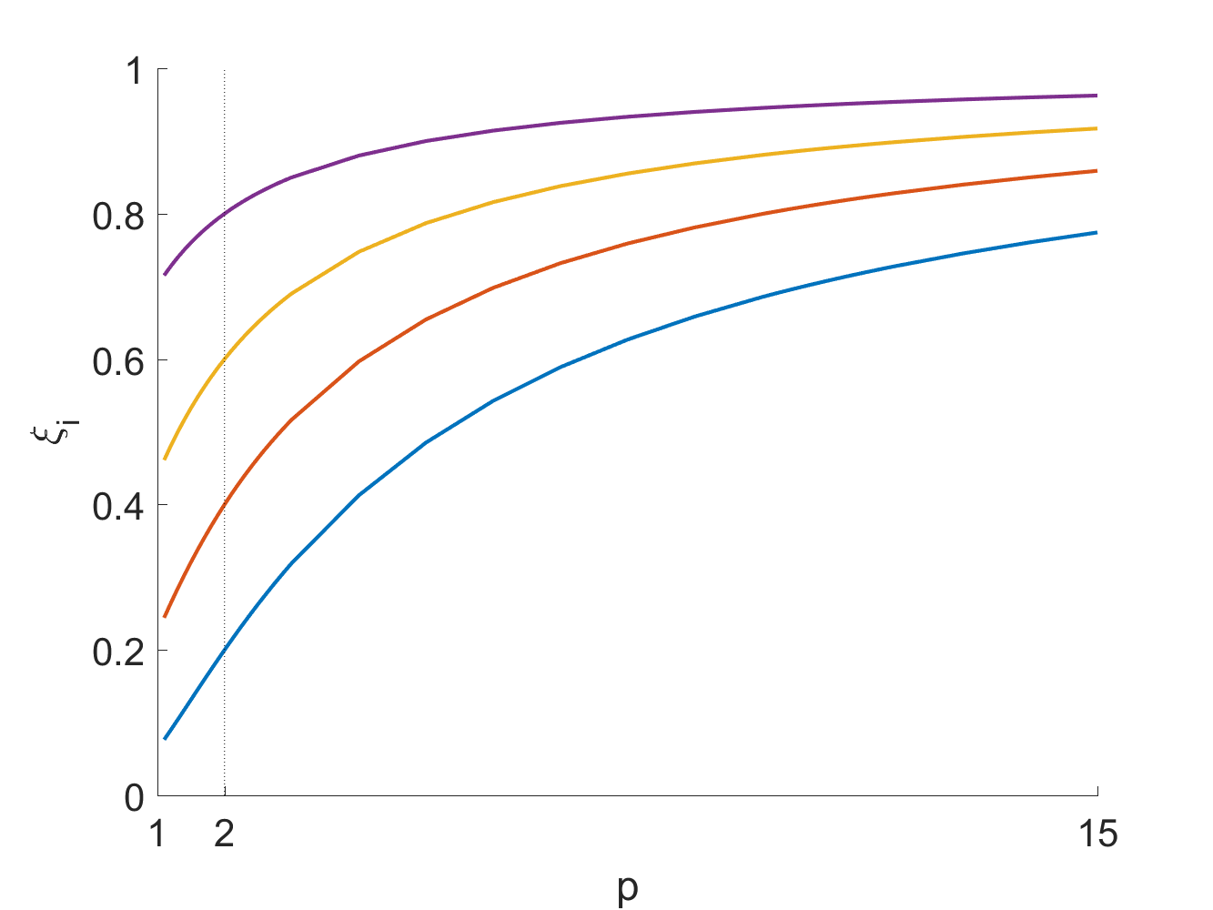
Figure 2: minimizing $\bm{\xi}$ for varying $p$ ($n=5$, $\ell=0$, $u=1$).

In fact, we can show that Newton’s method behaves very nicely on this function.

Proposition 12.

For the equally-spaced linearization points $\xi_{i}:=\ell+\frac{i}{n}(u-\ell)$, we have $F(\bm{\xi})>0$ when $1<p<2$, and $F(\bm{\xi})<0$ when $p>2$.

Proof.

We only need to prove the single-linearization-point case, because $\xi_{i}=\frac{\xi_{i-1}+\xi_{i+1}}{2}$ for $i-1,\ldots,n-1$. Let $\hat{\xi}_{1}(p)$ be the unique optimal solution for power $p$. Then $F(\hat{\xi}_{1}(p))=0$ and $\hat{\xi}_{1}(2)=\frac{\ell+u}{2}$ is the equally-spaced linearization point. By Lemma 7, we have that $F^{\prime}(\hat{\xi}_{1}(p))>0$.

For $1<p<2$, by Theorem 3.11, $\hat{\xi}_{1}(p)\leq\hat{\xi}_{1}(2)$. Therefore,

$$F(\hat{\xi}_{1}(2))\geq F(\hat{\xi}_{1}(p))+F^{\prime}(\hat{\xi}_{1}(p))(\hat{\xi}_{1}(2)-\hat{\xi}_{1}(p))\geq 0,$$

because of the convexity of $F(\xi_{1})$ (Lemma 8(i)).

For $p>2$, by Theorem 3.11, $\hat{\xi}_{1}(p)\geq\hat{\xi}_{1}(2)$. Therefore,

$$F(\hat{\xi}_{1}(2))\leq F(\hat{\xi}_{1}(p))+F^{\prime}(\hat{\xi}_{1}(p))(\hat{\xi}_{1}(2)-\hat{\xi}_{1}(p))\leq 0,$$

because of the concavity of $F(\xi_{1})$ (Lemma 8(ii)). ∎

Theorem 3.13.

Starting from an initial point $x^{0}=(\ell+\frac{(u-\ell)}{n},\dots,\ell+\frac{i(u-\ell)}{n},\dots,\ell+\frac{(n-1)(u-\ell)}{n})^{\top}$, construct the Newton’s-method sequence $\{x^{k}\}$ by iterating

$$x^{k+1}:=x^{k}-[F^{\prime}(x^{k})]^{-1}F(x^{k}).$$

Then $\{x^{k}\}$ is monotonically decreasing (increasing) to $x^{*}$ when $1<p<2$ (respectively, $p>2$), where $x^{*}$ satisfies $F(x^{*})=0$.

Proof.

The result follows from Lemma 7, Lemma 8 and the “Monotone Newton Theorem” (ortega2000iterative, , Theorem 13.3.4). In the Appendix, we provide a short direct proof. ∎

Remark 3.

For the case of a single non-boundary linearization point, the result also directly follows from the facts that $F^{\prime}(\xi_{1})\neq 0$ and $F(\xi_{1})F^{\prime\prime}(\xi_{1})>0$ for all $\xi_{1}$ between $x^{0}$ and $\hat{\xi}_{1}(p)$ (See mott1957newton ).

3.3 Optimal placement of a single non-boundary linearization point

It is interesting to make a detailed study of optimal placement of a single non-boundary linearization point, as it relates to necessary optimality conditions for $\bm{\xi}$, and it can give us a means to carry out a fast parallel coordinate-descent style algorithm. In this direction, we will establish that $\operatorname{vol}(\invbreve{U}^{*}_{p}(\ell,\xi_{1},u))$ has a unique minimizer.

Theorem 3.14.

• If $1<p\leq 2$, then $\operatorname{vol}(\invbreve{U}^{*}_{p}(\ell,\xi_{1},u))$ is strictly convex in $\xi_{1}$.

• If $p>2$, then $\operatorname{vol}(\invbreve{U}^{*}_{p}(\ell,\xi_{1},u))$ is quasiconvex in $\xi_{1}$.

Proof.

(i) follows directly from Theorem 3.5. (ii) follows directly from Theorem 3.4 (when $\frac{d}{d\xi_{1}}\operatorname{vol}(\invbreve{U}^{*}_{p}(\ell,\xi_{1},u))=0$, $\frac{d^{2}}{d\xi_{1}^{2}}\operatorname{vol}(\invbreve{U}^{*}_{p}(\ell,\xi_{1},u))>0$). ∎

We immediately have the following very-useful result.

Corollary 15.

For all $p>1$, $\operatorname{vol}(\invbreve{U}^{*}_{p}(\ell,\xi_{1},u))$ has a unique minimizer on $(\ell,u)$.

Proposition 16.

For all $p>2$, $\operatorname{vol}(\invbreve{U}^{*}_{p}(\ell,\xi_{1},u))$ is convex in $\xi_{1}$ to the right of the minimizer, and not convex near $\ell$.

Proof.

$$\frac{\partial^{2}\operatorname{vol}(\invbreve{U}^{*}_{p}(\ell,\xi_{1},u))}{\partial\xi_{1}^{2}}=\frac{p}{\xi_{1}}\frac{\partial\operatorname{vol}(\invbreve{U}^{*}_{p}(\ell,\xi_{1},u))}{\partial\xi_{1}}+\frac{\ell}{\xi_{1}}b_{\ell}+\frac{u}{\xi_{1}}b_{u},$$

where

$$~{}~{}\frac{p}{\xi_{1}}\frac{\partial\operatorname{vol}(\invbreve{U}^{*}_{p}(\ell,\xi_{1},u))}{\partial\xi_{1}}$$

$$=-\frac{(p-1)\xi_{1}^{p-2}}{6p}\left(\left(\frac{\xi_{1}^{p}+(p-1)u^{p}-p\xi_{1}u^{p-1}}{u^{p-1}-\xi_{1}^{p-1}}\right)^{2}-\left(\frac{\xi_{1}^{p}+(p-1)\ell^{p}-p\xi_{1}\ell^{p-1}}{\xi_{1}^{p-1}-\ell^{p-1}}\right)^{2}\right),$$

$$b_{\ell}=\frac{(p-1)^{2}}{3p}\frac{\xi_{1}^{p-2}\ell^{p-2}[(p-1)\xi_{1}^{p}+\ell^{p}-p\xi_{1}^{p-1}\ell)][\xi_{1}^{p}+(p-1)\ell^{p}-p\xi_{i}\ell^{p-1}]}{(\xi_{1}^{p-1}-\ell^{p-1})^{3}}>0,$$

$$b_{u}=\frac{(p-1)^{2}}{3p}\frac{\xi_{1}^{p-2}u^{p-2}[(p-1)\xi_{1}^{p}+u^{p}-p\xi_{1}^{p-1}u)][\xi_{1}^{p}+(p-1)u^{p}-p\xi_{1}u^{p-1}]}{(u^{p-1}-\xi_{1}^{p-1})^{3}}>0.$$

Suppose that $\xi_{1}^{*}$ is the minimizer of $\operatorname{vol}(\invbreve{U}^{*}_{p}(\ell,\xi_{1},u))$. By Theorem 3.17, we have that

$$\frac{\partial\log h_{p}(\xi_{1})}{\partial\xi_{1}}=-\frac{1}{h_{p}(\xi_{1})}\frac{\partial\operatorname{vol}(\invbreve{U}^{*}_{p}(\ell,\xi_{1},u))}{\partial\xi_{1}}$$

is decreasing on $(\ell,u)$. Therefore,

$$\frac{\partial\operatorname{vol}(\invbreve{U}^{*}_{p}(\ell,\xi_{1},u))}{\partial\xi_{1}}\left\{\begin{array}[]{ll}<0,&\hbox{for $\xi_{1}\in(\ell,\xi_{1}^{*})$ ;}\\ >0,&\hbox{for $\xi_{1}\in(\xi_{1}^{*},u)$.}\end{array}\right.$$

So $\frac{\partial^{2}\operatorname{vol}(\invbreve{U}^{*}_{p}(\ell,\xi_{1},u))}{\partial\xi_{1}^{2}}>0$ for $\xi_{1}\in(\xi_{1}^{*},u)$.

Next, we demonstrate that $\frac{\partial^{2}\operatorname{vol}(\invbreve{U}^{*}_{p}(\ell,\xi_{1},u))}{\partial\xi_{1}^{2}}$ can be negative near $\ell$ when $\ell/u$ is small enough. Notice that $\lim\limits_{\xi_{1}\rightarrow\ell}b_{\ell}=0$, and

$$\lim\limits_{\xi_{1}\rightarrow\ell}\frac{\partial\operatorname{vol}(\invbreve{U}^{*}_{p}(\ell,\xi_{1},u))}{\partial\xi_{1}}=-\frac{(p-1)\ell^{p-2}}{6p}\left(\frac{\ell^{p}+(p-1)u^{p}-p\ell u^{p-1}}{u^{p-1}-\ell^{p-1}}\right)^{2}.$$

Therefore,

$$\lim\limits_{\xi_{1}\rightarrow\ell}\frac{\partial^{2}\operatorname{vol}(\invbreve{U}^{*}_{p}(\ell,\xi_{1},u))}{\partial\xi_{1}^{2}}$$

$$=~{} -\frac{(p-1)\ell^{p-3}}{6}\left(\frac{\ell^{p}+(p-1)u^{p}-p\ell u^{p-1}}{u^{p-1}-\ell^{p-1}}\right)^{2}+\frac{u}{\ell}\lim\limits_{\xi_{1}\rightarrow\ell}b_{u}$$

$$=~{} -\frac{(p-1)\ell^{p-3}[(p-1)u^{p}+\ell^{p}-pu^{p-1}\ell]}{6p(u^{p-1}-\ell^{p-1})^{3}}$$

$$~{}\times\Big{[}(p-1)u^{p-1}[(p-2)(u^{p}-\ell^{p})-pu\ell(u^{p-2}-\ell^{p-2})]-p\ell(u^{p-1}-\ell^{p-1})^{2}\Big{]}$$

$$:=~{} -\frac{(p-1)\ell^{p-3}[(p-1)u^{p}+\ell^{p}-pu^{p-1}\ell]}{6p(u^{p-1}-\ell^{p-1})^{3}}u^{2p-1}k_{1}(\frac{\ell}{u}),$$

where $k_{1}(t):=(p-1)[(p-2)(1-t^{p})-p(t-t^{p-1})]-pt(1-t^{p-1})^{2}$. Notice that $\lim\limits_{t\rightarrow 0}k_{1}(t)=(p-1)(p-2)>0$, because $p>2$. Thus, when $\ell/u$ tends to $0$, $\frac{\partial^{2}\operatorname{vol}(\invbreve{U}^{*}_{p}(\ell,\xi_{1},u))}{\partial\xi_{1}^{2}}$ is negative. ∎

Even though $\operatorname{vol}(\invbreve{U}^{*}_{p}(\ell,\xi_{1},u))$ is not generally convex in $\xi_{1}$ for $p>2$, through a simple transformation, we can finds its unique minimizer (which we already know exists because it is quasiconvex) by equivalently maximizing a related strictly concave function.

Theorem 3.17.

If $p>2$, then $h_{p}(\xi_{1}):=C-\operatorname{vol}(\invbreve{U}^{*}_{p}(\ell,\xi_{1},u))$ is strictly log-concave, where

$$C=\frac{((p-1)u^{p}+\ell^{p}-pu^{p-1}\ell)(u^{p}+(p-1)\ell^{p}-pu\ell^{p-1})}{6p(u^{p-1}-\ell^{p-1})}.$$

Proof.

$h_{p}(\xi_{1})=\frac{(p-1)^{2}(u^{p-1}-\ell^{p-1})}{6p}q_{1}(\xi_{1})q_{2}(\xi_{1})$, where $q_{1}(x)=\left(\frac{u^{p}-\ell^{p}}{u^{p-1}-\ell^{p-1}}-\frac{x^{p}-\ell^{p}}{x^{p-1}-\ell^{p-1}}\right)$, and $q_{2}(x)=\left(\frac{x^{p}-u^{p}}{x^{p-1}-u^{p-1}}-\frac{u^{p}-\ell^{p}}{u^{p-1}-\ell^{p-1}}\right)$. We calculate

$$q_{1}^{\prime}(x) =-\frac{x^{p-2}[x^{p}-\ell^{p}-p\ell^{p-1}(x-\ell)]}{(x^{p-1}-\ell^{p-1})^{2}};$$

$$q_{1}^{\prime\prime}(x) =-\frac{(p-1)x^{p-3}\ell^{p-1}[(p-2)(x^{p}-\ell^{p})-p\ell x(x^{p-2}-\ell^{p-2})]}{(x^{p-1}-\ell^{p-1})^{3}}.$$

Similarly,

$$q_{2}^{\prime}(x) =\frac{x^{p-2}[x^{p}-u^{p}-pu^{p-1}(x-u)]}{(x^{p-1}-u^{p-1})^{2}};$$

$$q_{2}^{\prime\prime}(x) =\frac{(p-1)x^{p-3}u^{p-1}[(p-2)(x^{p}-u^{p})-pux(x^{p-2}-u^{p-2})]}{(x^{p-1}-u^{p-1})^{3}}.$$

Because of Lemma 1(ii) (See Appendix), $q_{1}^{\prime}(x)<0$, $q_{2}^{\prime}(x)>0$ on $(\ell,u)$. Thus $q_{1}(x)>q_{1}(u)=0$ and $q_{2}(x)>q_{2}(\ell)=0$. Because of Lemma 2(ii) (See Appendix), $q_{1}^{\prime\prime}(x)<0$, $q_{2}^{\prime\prime}(x)>0$.

We are going to show that $q_{1}(x)$ and $q_{2}(x)$ is strictly log-concave for $p>2$.

$$(\log q_{1}(x))^{\prime\prime}=\frac{q_{1}(x)q_{1}^{\prime\prime}(x)-(q_{1}^{\prime}(x))^{2}}{q_{1}(x)^{2}}<0.$$

Note that $q_{2}^{\prime\prime}(x)>0$ and $q_{2}(x)\leq\frac{x^{p}-u^{p}}{x^{p-1}-u^{p-1}}-u=\frac{x^{p-1}(x-u)}{x^{p-1}-u^{p-1}}$, thus

$$q_{2}(x)q_{2}^{\prime\prime}(x)-(q_{2}^{\prime}(x))^{2}$$

$$\leq~{} \frac{x^{p-1}(x-u)}{x^{p-1}-u^{p-1}}\frac{(p-1)x^{p-3}u^{p-1}[(p-2)(x^{p}-u^{p})-pux(x^{p-2}-u^{p-2})]}{(x^{p-1}-u^{p-1})^{3}}$$

$$-\frac{x^{2(p-2)}[x^{p}-u^{p}-pu^{p-1}(x-u)]^{2}}{(x^{p-1}-u^{p-1})^{4}}$$

$$=~{} \frac{x^{2(p-2)}}{(x^{p-1}-u^{p-1})^{4}}\Big{[}(p-1)u^{p-1}(x-u)[(p-2)(x^{p}-u^{p})-pux(x^{p-2}-u^{p-2})]$$

$$\phantom{blankblankblank}-[x^{p}-u^{p}-pu^{p-1}(x-u)]^{2}\Big{]}$$

$$= \frac{x^{2(p-2)}}{(x^{p-1}-u^{p-1})^{4}}\Big{[}-(p-1)u^{p-2}(x-u)^{2}[u^{p}-x^{p}-px^{p-1}(u-x)]$$

$$\phantom{blankblankblank}-x^{2}[(x^{p-1}-u^{p-1})^{2}-(p-1)^{2}u^{p-2}x^{p-2}(x-u)^{2}]\Big{]}.$$

By Lemma 1(ii) and Lemma 3(ii) (See Appendix), we have $(\log q_{2}(x))^{\prime\prime}<0$.

Therefore, $h_{p}(x)=\frac{(p-1)^{2}(u^{p-1}-\ell^{p-1})}{6p}q_{1}(x)q_{2}(x)$ is the product of two strictly log-concave function and is thus strictly log-concave. ∎

Next, we provide some bounds on the minimizing $\xi_{1}$. This can be useful for determining a reasonable initial point for a minimization algorithm (better than equally spaced) or even for a reasonable static rule for selecting linearization points. Additionally, we can see these bounds as necessary conditions for a minimizer.

Theorem 3.18.

For fixed $\ell$ and $u$, assume that $\xi_{1}$ minimizes $\operatorname{vol}(\invbreve{U}^{*}_{p}(\ell,\xi_{1},u))$, then

• if $p=2$, then $\xi_{1}=\frac{u+\ell}{2}$;

• if $1<p<2$, then

  $$\left(\frac{u^{p-1}+\ell^{p-1}}{2}\right)^{\frac{1}{p-1}}<\frac{(p-1)(u^{p}-\ell^{p})}{p(u^{p-1}-\ell^{p-1})}<\xi_{1}<\left(\frac{u^{p}-\ell^{p}}{p(u-\ell)}\right)^{\frac{1}{p-1}}<\frac{u+\ell}{2};$$

• if $p>2$, then

  $$\left(\frac{u^{p-1}+\ell^{p-1}}{2}\right)^{\frac{1}{p-1}}>\frac{(p-1)(u^{p}-\ell^{p})}{p(u^{p-1}-\ell^{p-1})}>\xi_{1}>\left(\frac{u^{p}-\ell^{p}}{p(u-\ell)}\right)^{\frac{1}{p-1}}>\frac{u+\ell}{2}.$$

Proof.

(i) follows directly from Theorem 3.1 when $n=2$. We only prove (ii), because (iii) follows a similar proof. $\xi_{1}$ satisfies the optimal condition $\frac{d}{d\xi_{1}}\operatorname{vol}(\invbreve{U}^{*}_{p}(\ell,\xi_{1},u))=0$, which is equivalent to

$$F(x):=\frac{x^{p}+(p-1)\ell^{p}-p\ell^{p-1}x}{x^{p-1}-\ell^{p-1}}-\frac{x^{p}+(p-1)u^{p}-pu^{p-1}x}{u^{p-1}-x^{p-1}}=0.$$

First, note that if $1<p<2$, and $x_{0}$ satisfies $F(x_{0})<0$, then $\xi_{1}>x_{0}$; if $x_{0}$ satisfies $F(x_{0})>0$, then $\xi_{1}<x_{0}$.

For the lower bound, notice that

$$F(x) =\frac{x^{p}+(p-1)\ell^{p}-p\ell^{p-1}x}{x^{p-1}-\ell^{p-1}}-\frac{x^{p}+(p-1)u^{p}-pu^{p-1}x}{u^{p-1}-x^{p-1}}$$

$$=-(x^{p}+(p-1)u^{p}-pu^{p-1}x)\left(\frac{1}{u^{p-1}-x^{p-1}}-\frac{1}{x^{p-1}-\ell^{p-1}}\right)$$

$$~{}~{}~{}~{}~{}~{}-\frac{(p-1)(u^{p}-\ell^{p})-p(u^{p-1}-\ell^{p-1})x}{x^{p-1}-\ell^{p-1}}.$$

Let $\underline{\xi}_{1}:=\frac{(p-1)(u^{p}-\ell^{p})}{p(u^{p-1}-\ell^{p-1})}$. To show $F(\underline{\xi}_{1})<0$, we only need to show that $\underline{\xi}_{1}^{p-1}-\ell^{p-1}>u^{p-1}-\underline{\xi}_{1}^{p-1}$, i.e., $\underline{\xi}_{1}>\left(\frac{u^{p-1}+\ell^{p-1}}{2}\right)^{\frac{1}{p-1}}$, which is the first inequality. Then we could conclude that $\xi_{1}>\underline{\xi}_{1}$.

To show the first inequality, we take logarithm on both sides and let $t:=\frac{\ell}{u}$. Then the inequality that we are going to prove is

$$J(t):=\log(1-t^{p})-\log(1-t^{p-1})+\log\frac{p-1}{p}-\frac{1}{p-1}(\log(t^{p-1}+1)-\log{2})>0$$

Notice that $\lim\limits_{t\rightarrow 1^{-}}J(t)=\log\frac{p}{p-1}+\log\frac{p-1}{p}=0$, and

$$J^{\prime}(t) =\frac{pt^{p-1}}{t^{p}-1}-\frac{(p-1)t^{p-2}}{t^{p-1}-1}-\frac{1}{p-1}\frac{(p-1)t^{p-2}}{t^{p-1}+1}$$

$$=\frac{t^{p-2}((p-2)(1-t^{p})-pt(1-t^{p-2}))}{(t^{p}-1)(t^{p-1}-1)(t^{p-1}+1)}.$$

By Lemma 2(i) (See Appendix), $J^{\prime}(t)<0$ on $(0,1)$. Thus $J(t)>0$ for $t\in(0,1)$.

For the upper bound, first we claim that for $0<t<1$, we have

$$\frac{t^{p}+(p-1)-pt}{1+(p-1)t^{p}-pt^{p-1}}>t^{\frac{2-p}{3}}.$$ (3)

To prove the claim, let $K(t):=t^{\frac{2-p}{3}}(1+(p-1)t^{p}-pt^{p-1})-t^{p}-(p-1)+pt$.

$$K^{\prime}(t) =\frac{2-p}{3}t^{-\frac{p+1}{3}}+(p-1)\frac{2(p+1)}{3}t^{\frac{2p-1}{3}}-p\frac{2p-1}{3}t^{\frac{2p-4}{3}}-pt^{p-1}+p$$

$$=t^{-\frac{p+1}{3}}\left(\frac{2-p}{3}+\frac{2(p-1)(p+1)}{3}t^{p}-\frac{p(2p-1)}{3}t^{p-1}-pt^{\frac{4p-2}{3}}+pt^{\frac{p+1}{3}}\right)$$

$$=:t^{-\frac{p+1}{3}}K_{1}(t).$$

$$K_{1}^{\prime}(t) =\frac{d}{dt}\left(t^{\frac{p+1}{3}}K^{\prime}(t)\right)$$

$$= \frac{2p(p^{2}-1)}{3}t^{p-1}-\frac{p(p-1)(2p-1)}{3}t^{p-2}-\frac{p(4p-2)}{3}t^{\frac{4p-5}{3}}+\frac{p(p+1)}{3}t^{\frac{p-2}{3}}$$

$$= \frac{p}{3}t^{\frac{p-2}{3}}\left(2(p^{2}-1)t^{\frac{2p-1}{3}}-(2p-1)(p-1)t^{\frac{2p-4}{3}}-2(2p-1)t^{p-1}+(p+1)\right)$$

$$=: \frac{p}{3}t^{\frac{p-2}{3}}K_{2}(t).$$

$$K_{2}^{\prime}(t) =\frac{d}{dt}\left(\frac{3}{p}t^{\frac{2-p}{3}}\frac{d}{dt}\left(t^{\frac{p+1}{3}}K^{\prime}(t)\right)\right)$$

$$= 2(2p-1)(p-1)t^{\frac{2p-7}{3}}\left(\frac{p+1}{3}t-\frac{p-2}{3}-t^{\frac{p+1}{3}}\right)$$

$$= -2(2p-1)(p-1)t^{\frac{2p-7}{3}}\left((t^{\frac{p+1}{3}}-1)-\frac{p+1}{3}(t-1)\right)>0.$$

The last inequality follows from the strict concavity of function $x^{\frac{p+1}{3}}$ when $1<p<2$. Because $K_{2}(1)=0$, we have $K_{2}(t)<0$ on $(0,1)$, which implies $K_{1}(t)$ is decreasing on $(0,1)$. Along with $K_{1}(1)=0$, which implies $K_{1}(t)>0$ on $(0,1)$. Therefore, $K(t)$ is increasing on $(0,1)$, and $K(t)<K(1)=0$, which proves the claim.

Letting $\overline{\xi}_{1}:=\left(\frac{u^{p}-\ell^{p}}{p(u-\ell)}\right)^{\frac{1}{p-1}}$, and $t:=\frac{\ell}{u}$, we have

$$\ell^{p}-p\overline{\xi}_{1}^{p-1}\ell=u^{p}-p\overline{\xi}_{1}^{p-1}u,$$

$$\frac{\overline{\xi}_{1}^{p-1}-\ell^{p-1}}{u^{p-1}-\overline{\xi}_{1}^{p-1}}=\frac{p(u-\ell)(\overline{\xi}_{1}^{p-1}-\ell^{p-1})}{p(u-\ell)(u^{p-1}-\overline{\xi}_{1}^{p-1})}=\frac{(p-1)t^{p}+1-pt^{p-1}}{t^{p}+(p-1)-pt}.$$

We are going to show that $F(\overline{\xi}_{1})>0$. Letting $h(x):=\frac{x^{p}+(p-1)-px}{x(x^{p-1}-1)}$, we have

$$h^{\prime}(x)=\frac{(p-1)((p-1)x^{p}+1-px^{p-1})}{x^{2}(x^{p-1}-1)^{2}},$$

and

$$H(t):=\frac{F(\overline{\xi}_{1})}{\overline{\xi}_{1}} =h\left(\frac{\overline{\xi}_{1}}{\ell}\right)+h\left(\frac{\overline{\xi}_{1}}{u}\right)$$

$$=h\left(\left(\frac{(t^{p}-1)}{pt^{p-1}(t-1)}\right)^{\frac{1}{p-1}}\right)+h\left(\left(\frac{(t^{p}-1)}{p(t-1)}\right)^{\frac{1}{p-1}}\right).$$

$$\frac{dH(t)}{dt} =-h^{\prime}\left(\frac{\overline{\xi}_{1}}{\ell}\right)\frac{1}{p-1}\left(\frac{\overline{\xi}_{1}}{\ell}\right)^{2-p}\frac{t^{p}+(p-1)-pt}{pt^{p}(t-1)^{2}}$$

$$~{}~{}~{}~{}~{}+h^{\prime}\left(\frac{\overline{\xi}_{1}}{u}\right)\frac{1}{p-1}\left(\frac{\overline{\xi}_{1}}{u}\right)^{2-p}\frac{(p-1)t^{p}+1-pt^{p-1}}{p(t-1)^{2}}$$

$$=-\frac{\ell^{p-2}}{p(t-1)^{2}}\left(\frac{\overline{\xi}_{1}}{u}\right)^{-p}\frac{((p-1)\overline{\xi}_{1}^{p}+\ell^{p}-p\overline{\xi}_{1}^{p-1}\ell)(t^{p}+(p-1)-pt)}{(\overline{\xi}_{1}^{p-1}-\ell^{p-1})^{2}}$$

$$~{}~{}~{}~{}~{}+\frac{u^{p-2}}{p(t-1)^{2}}\left(\frac{\overline{\xi}_{1}}{u}\right)^{-p}\frac{((p-1)\overline{\xi}_{1}^{p}+u^{p}-p\overline{\xi}_{1}^{p-1}u)((p-1)t^{p}+1-pt^{p-1})}{(u^{p-1}-\overline{\xi}_{1}^{p-1})^{2}}$$

$$=\frac{\ell^{p-2}}{p(t-1)^{2}}\left(\frac{\overline{\xi}_{1}}{u}\right)^{-p}((p-1)\overline{\xi}_{1}^{p}+\ell^{p}-p\overline{\xi}_{1}^{p-1}\ell)$$

$$~{}~{}~{}~{}~{}\times\left(-\frac{(t^{p}+(p-1)-pt)}{(\overline{\xi}_{1}^{p-1}-\ell^{p-1})^{2}}+\frac{t^{2-p}((p-1)t^{p}+1-pt^{p-1})}{(u^{p-1}-\overline{\xi}_{1}^{p-1})^{2}}\right)$$

$$=\frac{\ell^{p-2}}{p(t-1)^{2}}\left(\frac{\overline{\xi}_{1}}{u}\right)^{-p}((p-1)\overline{\xi}_{1}^{p}+\ell^{p}-p\overline{\xi}_{1}^{p-1}\ell)$$

$$~{}~{}~{}~{}~{}\times\frac{(p-1)t^{p}+1-pt^{p-1}}{(u^{p-1}-\overline{\xi}_{1}^{p-1})^{2}}\left(t^{2-p}-\left(\frac{t^{p}+(p-1)-pt}{(p-1)t^{p}+1-pt^{p-1}}\right)^{3}\right)<0.$$

The last inequality follows from (3). Therefore, along with $\lim\limits_{t\rightarrow 1^{-}}H(t)=0$, we have $H(t)>0$ for $t\in(0,1)$, which implies $F(\overline{\xi}_{1})>0$ and $\xi_{1}<\overline{\xi}_{1}$.

To show that $\frac{u+\ell}{2}>\overline{\xi}_{1},$ we take logarithm on both sides and let $t:=\frac{\ell}{u}$. Then the inequality that we are going to prove is

$$L(t):=\log(1-t^{p})-\log(1-t)-\log p-(p-1)(\log(t+1)-\log{2})<0.$$

Notice that $\lim\limits_{t\rightarrow 1^{-}}L(t)=0$, and

$$L^{\prime}(t) =\frac{pt^{p-1}}{t^{p}-1}-\frac{1}{t-1}-\frac{p-1}{t+1}$$

$$=\frac{(p-2)(t^{p}-1)-pt(t^{p-2}-1)}{(t^{p}-1)(t^{2}-1)}.$$

By Lemma 2(i) (See Appendix), $L^{\prime}(t)>0$ on $(0,1)$. Thus $L(t)<0$ for $t\in(1,\infty)$. ∎

Just as we determined the optimal location of a linearization point as $p$ varies (Theorem 3.11), we now determine the behavior of these bounds (Theorem 3.18) when $p$ varies. Toward this goal, let $t:=\frac{\ell}{u}$, and let

$$\Delta(p,t):=\frac{\overline{\xi}_{1}-\underline{\xi}_{1}}{u-\ell}=\frac{1}{1-t}\left(\left(\frac{1-t^{p}}{p(1-t)}\right)^{\frac{1}{p-1}}-\frac{(p-1)(1-t^{p})}{p(1-t^{p-1})}\right),$$

where $\underline{\xi}_{1}:=\frac{(p-1)(u^{p}-\ell^{p})}{p(u^{p-1}-\ell^{p-1})}$ and $\overline{\xi}_{1}:=\left(\frac{u^{p}-\ell^{p}}{p(u-\ell)}\right)^{\frac{1}{p-1}}$. We will demonstrate that the behavior of $\Delta(p,t)$ can be bounded, in a useful way, by the behavior of $\Delta(p,0)$. Then we will analyze $\Delta(p,0)$.

Theorem 3.19.

• For $1<p<2$, $\Delta(p,t)$ is decreasing in $t$, implying that $0<\Delta(p,t)\leq\Delta(p,0)$;

• for $p>2$, $(1-t)\Delta(p,t)$ is increasing in $t$, implying that $0>(1-t)\Delta(p,t)\geq\Delta(p,0)$.

Proof.

(i) We will demonstrate that the derivative of $\Delta(p,t)$ is negative when $1<p<2$.

$$\frac{\partial\Delta(p,t)}{\partial t} =\frac{1}{(1-t)^{2}}\left[\frac{\overline{\xi}_{1}}{\underline{\xi}_{1}}-\left(\frac{(p-1)^{2}t^{p-2}(1-t)^{2}}{p(1-t^{p-1})^{2}}+\frac{p-1}{p}\right)\right].$$

Let $\chi(t):=\log\left(\frac{\overline{\xi}_{1}}{\underline{\xi}_{1}}\right)-\log\left(\frac{(p-1)^{2}t^{p-2}(1-t)^{2}}{p(1-t^{p-1})^{2}}+\frac{p-1}{p}\right)$. Then

$$\frac{\partial\chi(t)}{\partial t} =\frac{(1-t^{p-1})^{2}-(p-1)^{2}t^{p-2}(1-t)^{2}}{(p-1)(1-t)(1-t^{p-1})(1-t^{p})}-\frac{(p-1)t^{p-3}(1-t)[(p-2)(1-t^{p})-p(t-t^{p-1})]}{(1-t^{p-1})[(1-t^{p-1})^{2}+(p-1)t^{p-2}(1-t)^{2}]}.$$

We claim that

$$0>\frac{(1-t^{p-1})^{2}-(p-1)^{2}t^{p-2}(1-t)^{2}}{(p-1)(1-t)}>\frac{(p-2)(1-t^{p})-p(t-t^{p-1})}{2t}.$$

Then

$$\frac{\partial\chi(t)}{\partial t} >\frac{(p-2)(1-t^{p})-p(t-t^{p-1})}{t(1-t^{p-1})(1-t^{p})}\left(\frac{1}{2}-\frac{(p-1)t^{p-2}(1-t)(1-t^{p})}{(1-t^{p-1})^{2}+(p-1)t^{p-2}(1-t)^{2}}\right)$$

$$=\frac{(p-2)(1-t^{p})-p(t-t^{p-1})}{t(1-t^{p-1})(1-t^{p})}\left(\frac{1}{2}-\frac{(p-1)t^{p-2}(1-t)(1-t^{p})}{(1-t^{p-1})^{2}+(p-1)t^{p-2}(1-t)^{2}}\right).$$

Notice that $(p-2)(1-t^{p})-p(t-t^{p-1})<0$, and

$$\frac{(p-1)t^{p-2}(1-t)(1-t^{p})}{(1-t^{p-1})^{2}+(p-1)t^{p-2}(1-t)^{2}} >\frac{(p-1)t^{p-2}(1-t)(1-t^{p})}{(p-1)^{2}t^{p-2}(1-t)^{2}+(p-1)t^{p-2}(1-t)^{2}}$$

$$=\frac{1-t^{p}}{p(1-t)}>\frac{1}{p}>\frac{1}{2}.$$

Therefore, $\frac{\partial\chi(t)}{\partial t}>0$, and hence $\chi(t)<\lim_{t\rightarrow 1^{-}}\chi(t)=0$, i.e., $\frac{\partial\Delta(p,t)}{\partial t}<0$.

What remains is to prove the claim. By Lemma 2(i) and Lemma 3(i) (See Appendix), we have that the two terms are both negative on $(0,1)$. Letting

$$\Theta(t):=2t[(1-t^{p-1})^{2}-(p-1)^{2}t^{p-2}(1-t)^{2}]-(p-1)(1-t)[(p-2)(1-t^{p})-p(t-t^{p-1})],$$

we have

$$\Theta^{\prime}(t) =2(2p-1)t^{2p-2}-(p^{2}-1)(3p-4)t^{p}+2p(3(p-1)^{2}-2)t^{p-1}$$

$$~{}~{}~{}~{}-(p-1)^{2}(3p-2)t^{p-2}-2p(p-1)t+(2p^{2}-4p+4).$$

$$\Theta^{\prime\prime}(t) =(p-1)[4(2p-1)t^{2p-3}-p(p+1)(3p-4)t^{p-1}+2p(3(p-1)^{2}-2)t^{p-2}$$

$$~{}~{}~{}~{}\phantom{(p-1)}-(p-1)(3p-2)(p-2)t^{p-3}-2p].$$

$$\Theta^{\prime\prime\prime}(t) =(p-1)t^{p-4}[4(2p-1)(2p-3)t^{p}-p(p+1)(3p-4)(p-1)t^{2}$$

$$~{}~{}~{}~{}\phantom{(p-1)t^{p-4}}+2p(3(p-1)^{2}-2)(p-2)t-(p-1)(3p-2)(p-2)(p-3)]$$

$$=(p-1)t^{p-4}\Big{[}2(p-1)^{2}[6t^{p}-p(p+1)t^{2}+2p(p-2)t-(p-2)(p-3)]$$

$$~{}~{}~{}~{}\phantom{(p-1)t^{p-4}}+p(p-2)[4t^{p}-(p^{2}-1)t^{2}+2(p^{2}-2p-1)t-(p-3)(p-1)]\Big{]}.$$

Let $\Theta_{1}(t):=6t^{p}-p(p+1)t^{2}+2p(p-2)t-(p-2)(p-3)$, $\Theta_{2}(t):=4t^{p}-(p^{2}-1)t^{2}+2(p^{2}-2p-1)t-(p-3)(p-1)$. We first show that $t^{p}-1-p(t-1)\leq(p-1)(1-t)^{2}$. This follows from the fact that

$$\frac{d}{dt}\left(\frac{t^{p}-1-p(t-1)}{(1-t)^{2}}\right)=\frac{(p-2)(1-t^{p})-p(t-t^{p-1})}{(1-t)^{3}}<0\quad\text{(Lemma~{}\ref{lem:hx}(i), See Appendix)}.$$

Then we have

$$\Theta_{1}(t) =6(t^{p}-1-p(t-1))-p(p+1)(1-t)^{2}$$

$$\leq 6(p-1)(1-t)^{2}-p(p+1)(1-t)^{2}$$

$$=-(p-2)(p-3)(1-t)^{2}<0.$$

$$\Theta_{2}^{\prime}(t) =4pt^{p-1}-2(p^{2}-1)t+2(p^{2}-2p-1).$$

$$\Theta_{2}^{\prime\prime}(t) =2(p-1)t^{p-2}(2p-(p+1)t^{2-p})>0.$$

Thus $\Theta_{2}^{\prime}(t)<\Theta_{2}^{\prime}(1)=0$, which implies $\Theta_{2}(t)$ is decreasing and $\Theta_{2}(t)>\Theta_{2}(1)=0$. Because $\Theta_{1}(t)<0$ and $\Theta_{2}(t)>0$, we have that $\Theta^{\prime\prime\prime}(t)<0$. Therefore, $\Theta^{\prime\prime}(t)>\Theta^{\prime\prime}(1)=0$, which implies that $\Theta^{\prime}(t)$ is increasing. Thus $\Theta^{\prime}(t)<\Theta^{\prime}(1)=0$, which that implies $\Theta(t)$ is decreasing, i.e., $\Theta(t)>\Theta(1)=0$. Then the claim follows directly.

(ii) When $p>2$, notice that the derivative of $\Delta(p,t)$ at $t=0$ is

$$\lim_{t\rightarrow 0^{+}}\frac{\partial\Delta(p,t)}{\partial t}=\frac{\left(\frac{1}{p}\right)^{\frac{1}{p-1}}}{\frac{p-1}{p}}-\frac{p-1}{p}.$$

When $p>6.236$, the derivative would become negative. Therefore, we could not expect that $\Delta(p,t)$ is increasing when $p>6.236$.

Instead, we are going to show that the function $(1-t)\Delta(p,t)$ is increasing. Its derivative is

$$\left(\frac{1-t^{p}}{p(1-t)}\right)^{\frac{1}{p-1}}\frac{(p-1)t^{p}+1-pt^{p-1}}{(p-1)(1-t^{p})(1-t)}-\frac{(p-1)t^{p-2}(t^{p}+p-1-pt)}{p(1-t^{p-1})^{2}}.$$

We are going to demonstrate that this derivative is positive. Let

$$\Omega(t) :=\log\left(\left(\frac{1-t^{p}}{p(1-t)}\right)^{\frac{1}{p-1}}\frac{(p-1)t^{p}+1-pt^{p-1}}{(p-1)(1-t^{p})(1-t)}\right)-\log\left(\frac{(p-1)t^{p-2}(t^{p}+p-1-pt)}{p(1-t^{p-1})^{2}}\right)$$

$$=\log\left(\left(\frac{1-t^{p}}{p(1-t)}\right)^{\frac{1}{p-1}}\right)-\log\left(\frac{(p-1)(1-t^{p})}{p(1-t^{p-1})}\right)-\log\left(\frac{(p-1)t^{p-2}(1-t)(t^{p}+p-1-pt)}{(1-t^{p-1})((p-1)t^{p}+1-pt^{p-1})}\right).$$

$$\Omega^{\prime}(t) =\frac{(1-t^{p-1})^{2}-(p-1)^{2}t^{p-2}(1-t)^{2}}{(p-1)(1-t)(1-t^{p-1})(1-t^{p})}-\frac{(p-2)-(p-1)t+t^{p-1}}{t(1-t)(1-t^{p-1})}$$

$$~{}~{}~{}~{}+\frac{p[(1-t^{p-1})^{2}-(p-1)^{2}t^{p-2}(1-t)^{2}]}{((p-1)t^{p}+1-pt^{p-1})(t^{p}+p-1-pt)}$$

$$=\frac{(1-t^{p-1})^{2}-(p-1)^{2}t^{p-2}(1-t)^{2}}{(p-1)(1-t)(1-t^{p-1})(1-t^{p})}-\frac{t^{p}+(p-1)-pt}{t(1-t)((p-1)t^{p}+1-pt^{p-1})}$$

$$~{}~{}~{}~{}+\frac{(p-1)((p-1)t^{p}+1-pt^{p-1})}{t(1-t^{p-1})(t^{p}+(p-1)-pt)}$$

$$=\frac{p[(1-t^{p-1})^{2}-(p-1)^{2}t^{p-2}(1-t)^{2}]}{(p-1)(1-t)(1-t^{p})((p-1)t^{p}+1-pt^{p-1})}$$

$$~{}~{}~{}~{}-\frac{(p-1)((p-2)(1-t^{p})-p(t-t^{p-1}))}{t(1-t^{p-1})(t^{p}+(p-1)-pt)}.$$

We claim that

$$0<\frac{p[(1-t^{p-1})^{2}-(p-1)^{2}t^{p-2}(1-t)^{2}]}{(p-1)(1-t^{p})}<\frac{(p-2)(1-t^{p})-p(t-t^{p-1})}{t}.$$

Then

$$\Omega^{\prime}(t) <\frac{(p-2)(1-t^{p})-p(t-t^{p-1})}{t(1-t^{p-1})(1-t)}\left(\frac{1-t^{p-1}}{(p-1)t^{p}+1-pt^{p-1}}-\frac{(p-1)(1-t)}{t^{p}+(p-1)-pt}\right)$$

$$=\frac{(p-2)(1-t^{p})-p(t-t^{p-1})}{t(1-t^{p-1})(1-t)}\left(\frac{-t[(1-t^{p-1})^{2}-(p-1)^{2}t^{p-2}(1-t)^{2}]}{((p-1)t^{p}+1-pt^{p-1})(t^{p}+(p-1)-pt)}\right)<0.$$

Therefore, $\Omega(t)>\lim_{t\rightarrow 1^{-}}\Omega(t)=0$, i.e., the derivative of $(1-t)\Delta(p,t)$ is positive.

We only need to prove the claim. Letting

$$\Phi(t):=pt[(1-t^{p-1})^{2}-(p-1)^{2}t^{p-2}(1-t)^{2}]-(p-1)(1-t^{p})[(p-2)(1-t^{p})-p(t-t^{p-1})],$$

we have

$$\Phi^{\prime}(t) =p[-2(p-1)(p-2)t^{2p-1}+p(2p-1)t^{2p-2}-p(p^{2}-1)t^{p}$$

$$~{}~{}~{}~{}+2(p-2)(p^{2}+p-1)t^{p-1}-p(p-1)^{2}t^{p-2}+p].$$

$$\Phi^{\prime\prime}(t) =p(p-1)t^{p-3}[-2(p-2)(2p-1)t^{p+1}+2p(2p-1)t^{p}-p^{2}(p+1)t^{2}$$

$$~{}~{}~{}~{}\phantom{p(p-1)t^{p-3}}+2(p-2)(p^{2}+p-1)t-p(p-1)(p-2)].$$

Let $\Phi_{1}(t):=\frac{\Phi^{\prime\prime}(t)}{p(p-1)t^{p-3}}=2(p-2)(2p-1)t^{p+1}+2p(2p-1)t^{p}-p^{2}(p+1)t^{2}+2(p-2)(p^{2}+p-1)t-p(p-1)(p-2)$. Then

$$\Phi_{1}^{\prime}(t) =-2(p-2)(2p-1)(p+1)t^{p}+2p^{2}(2p-1)t^{p-1}-2p^{2}(p+1)t+2(p-2)(p^{2}+p-1);$$

$$\Phi_{1}^{\prime\prime}(t) =-2(p-2)(2p-1)(p+1)pt^{p-1}+2p^{2}(2p-1)(p-1)t^{p-2}-2p^{2}(p+1);$$

$$\Phi_{1}^{\prime\prime\prime}(t) =-2p(p-2)(2p-1)(p-1)t^{p-3}[(p+1)t-p].$$

Therefore, we have that $\Phi_{1}^{\prime\prime}(t)$ is increasing on $(0,\frac{p}{p+1})$ and decreasing on $(\frac{p}{p+1},1)$. We have $\Phi_{1}^{\prime\prime}(t)\leq\Phi_{1}^{\prime\prime}(\frac{p}{p+1})=2p^{2}(2p-1)\left(\frac{p}{p+1}\right)^{p-2}-2p^{2}(p+1)$. Letting $\Phi_{2}(p):=(p-2)\log\left(\frac{p}{p+1}\right)-\log\left(\frac{p+1}{2p-1}\right)$, we have

$$\Phi_{2}^{\prime}(p) =\frac{p-2}{p}+\log(p)-\frac{p-1}{p+1}-\log(p+1)+\frac{2}{2p-1};$$

$$\Phi_{2}^{\prime\prime}(p) =\frac{(p-2)(8p^{2}+p-1)}{p^{2}(p+1)^{2}(2p-1)^{2}}.$$

Therefore $\Phi_{2}^{\prime}(p)$ is increasing on $(2,\infty)$. Along with $\lim_{p\rightarrow\infty}\Phi_{2}^{\prime}(p)=0$, we have that $\Phi_{2}^{\prime}(p)<0$ on $(2,\infty)$, which implies that $\Phi_{2}(p)<\Phi_{2}(2)=0$. Thus $\Phi_{1}^{\prime\prime}(t)<0$. Then we have that $\Phi_{1}^{\prime}(t)$ is decreasing on $(0,1)$, which implies that $\Phi_{1}^{\prime}(t)>\Phi_{1}^{\prime}(1)=0$. Therefore, we have $\Phi_{1}(t)<\Phi_{1}(1)=0$, i.e., $\Phi^{\prime\prime}(t)<0$. Then we conclude that $\Phi^{\prime}(t)$ is decreasing on $(0,1)$, which implies that $\Phi^{\prime}(t)>\Phi(1)=0$. Therefore, $\Phi(t)$ is increasing on $(0,1)$ and $\Phi(t)<\Phi(1)=0$, which proves the claim. ∎

Because of Theorem 3.19, we can focus on the special case $\ell=0$. So we define

$$\Delta(p):=\Delta(p,0)=\left(\frac{1}{p}\right)^{\frac{1}{p-1}}-\frac{p-1}{p}.$$

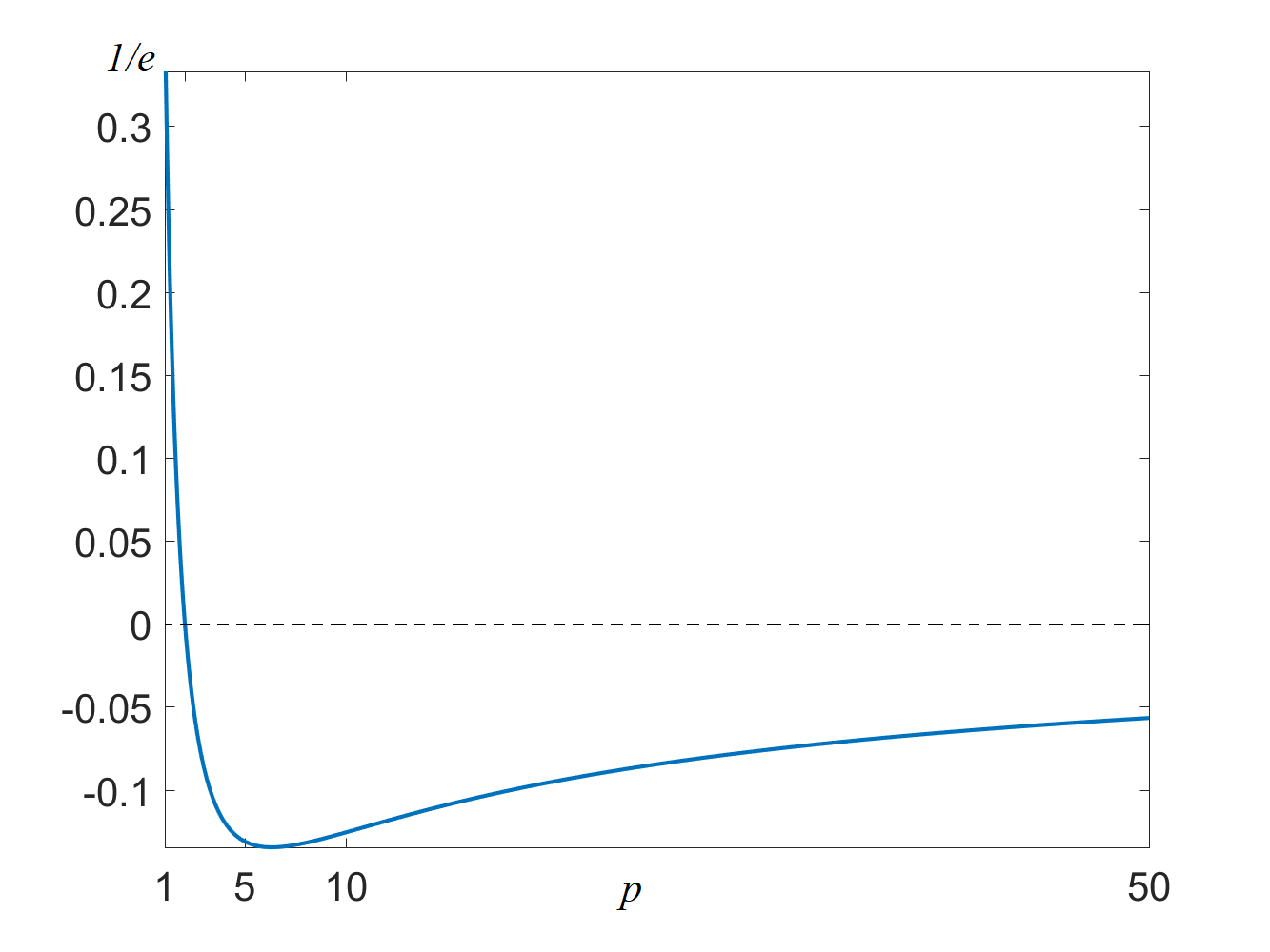
Figure 3: $\Delta(p)$

From Figure 3, we can see the behavior of $\Delta(p)$, which is summarized in the following result.

Proposition 20.

$\Delta(p)$ $(p>1)$ satisfies the following properties:

• $\Delta(p)>0$ when $1<p<2$; $\Delta(2)=0$; and $\Delta(p)<0$ when $p>2$;

• $\lim\limits_{p\rightarrow 1}\Delta(p)=e^{-1}$; $\lim\limits_{p\rightarrow\infty}\Delta(p)=0$;

• $\Delta(p)$ is minimized at $p_{0}$, where $p_{0}\approx 6.3212$;

• $0.3679\approx e^{-1}\geq\Delta(p)\geq\Delta(p_{0})\approx-0.1347$.

Proof.

(i) follows from Theorem 3.18. For (ii),

$$\lim\limits_{p\rightarrow 1}\Delta(p)=\lim\limits_{p\rightarrow 1}\exp\left\{-\frac{\log p}{p-1}\right\}=\exp\left\{-1\right\};\lim\limits_{p\rightarrow\infty}\Delta(p)=\lim\limits_{p\rightarrow\infty}\exp\left\{-\frac{\log p}{p-1}\right\}-1=0.$$

For (iii), we have

$$\Delta^{\prime}(p) =\left(\frac{1}{p}\right)^{\frac{1}{p-1}}\left[-\frac{1}{p(p-1)}+\frac{\log p}{(p-1)^{2}}\right]-\frac{1}{p^{2}}$$

$$=\left(\frac{1}{p}\right)^{\frac{1}{p-1}}\frac{1}{p^{2}}\left[-\frac{p}{p-1}+\frac{p^{2}\log p}{(p-1)^{2}}-p^{\frac{1}{p-1}}\right].$$

Notice that

$$\frac{d}{dp}\left(p^{2+\frac{1}{p-1}}\Delta^{\prime}(p)\right) =\frac{p^{2}-1-2p\log p}{(p-1)^{3}}-p^{\frac{1}{p-1}}\frac{(p-1)-p\log p}{p(p-1)^{2}}~{}>~{}0.$$

This follows from $p^{2}-1-2p\log p>0$ and $(p-1)-p\log p>0$ for $p>1$. Therefore, $p^{2+\frac{1}{p-1}}\Delta^{\prime}(p)$ is increasing on $(1,\infty)$. There exists unique $p_{0}>1$ satisfying

$$-\frac{p_{0}}{p_{0}-1}+\frac{p_{0}^{2}\log p_{0}}{(p_{0}-1)^{2}}-p_{0}^{\frac{1}{p_{0}-1}}=0,$$

and $\Delta^{\prime}(p)<0$ for $1<p<p_{0}$, $\Delta^{\prime}(p)>0$ for $p>p_{0}$, which implies that $\Delta(p_{0})=\min_{p>1}\Delta(p)$. (iv) follows directly. ∎

4 Lighter relaxations

As we mentioned at the outset, an alternative key relaxation previously studied requires that the domain of $f$ is all of $[0,u]$, $f$ is convex on $[0,u]$, $f(0)=0$, and $f$ is increasing on $[0,u]$. Assuming these properties, we recall the definition of the naïve relaxation

$$\invbreve{S}^{0}_{f}(\ell,u):=\left\{(x,y,z)\in\mathbb{R}^{3}~{}:~{}\left(f(\ell)-{\scriptstyle\frac{f(u)-f(\ell)}{u-\ell}}\ell\right)z+{\scriptstyle\frac{f(u)-f(\ell)}{u-\ell}}x\geq y\geq f(x),~{}\right.$$

$$\left.uz\geq x\geq\ell z,~{}1\geq z\geq 0\vphantom{\scriptstyle\frac{f(u)-f(\ell)}{u-\ell}}\right\}.$$

For example, convex power functions $f(x):=x^{p}$ on $[\ell,u]$, $\ell\geq 0$, with $p>1$ have the required properties. We wish to discuss a few different ways to handle functions $f$ with these properties.

• Naïve Relaxation [NR]: $\invbreve{S}^{0}_{f}(\ell,u)$

• Perspective Relaxation [PR]: $\invbreve{S}^{*}_{f}(\ell,u)$

• Piecewise-Linear under-est. $+$ Perspective Relaxation [PL+PR]: $\invbreve{U}^{*}_{f}(\bm{\xi}):=\invbreve{S}^{*}_{g}(\ell,u)$

• linearly Extend to 0 $+$ Naïve Relaxation [E+NR]: $\invbreve{S}^{0}_{\bar{f}}(\ell,u)$

• Piecewise-Linear under-est. $+$ linearly Extend to 0 $+$ Naïve Relaxation [PL+E+NR]: $\invbreve{U}^{0}_{\bar{f}}(\bm{\xi}):=\invbreve{S}^{0}_{\bar{g}}(\ell,u)$

One of the main focuses of Perspec2019 was comparing NR and PR, with the idea that PR is tighter than NR, but PR is more burdensome computationally. So far in this work, we have extensively investigated PL+PR, again with the motivation that PL+PR is less burdensome than PR. Because piecewise-linearization requires choosing linearization points, we have put a big emphasis on how to do that. When $\ell>0$, a simple way to do something stronger than NR is with E+NR: linearly interpolate on $[0,\ell]$ before applying the naïve relaxation — the strict convexity of the power function makes this stronger than NR. Finally, again when $\ell>0$, we can consider PL+E+NR: applying piecewise-linearization on $[\ell,u]$, linearly interpolating on $[0,\ell]$, and then applying the naïve relaxation.

In what follows, we focus on power functions, but the ideas could also be applied to other functions having the required properties.

4.1 PL+E+NR

Defining the piecewise-linear $g$ with respect to $f$ having domain $[\ell,u]$, we can extend $g$ to the function $\bar{g}$, with domain all of $[0,u]$:

$$\bar{g}(x):=\left\{\begin{array}[]{ll}\frac{f(\ell)}{\ell}x,&x\in[0,\ell);\\ g(x),&x\in[\ell,u].\end{array}\right.$$

In this way, $\bar{g}$ is a piecewise-linear increasing function on all of $[0,u]$, and is convex on $[0,u]$ as long as $f^{\prime}(\ell)\geq\frac{f(\ell)}{\ell}$. In fact, $\bar{g}$ is an under-estimator of the function that is $f$ on $[\ell,u]$ and 0 at 0. Next we calculate the volume of the naïve relaxation of the piecewise-linear under-estimator $\invbreve{U}^{0}_{\bar{f}}(\bm{\xi}):=\invbreve{S}^{0}_{\bar{g}}(\ell,u)$, by applying (Perspec2019, , Thm. 10) to $\bar{g}$.

Proposition 1.

Suppose that $f$ is convex and increasing on $[\ell,u]$ with $f^{\prime}(\ell)\geq\frac{f(\ell)}{\ell}$. For $\bm{\xi}=(\ell,\xi_{1},\dots,\xi_{n-1},u)$, where $f$ is differentiable at each coordinate of $\bm{\xi}$, we can compute $\invbreve{U}^{0}_{\bar{f}}(\bm{\xi})$ in $\mathcal{O}(n)$ time.

Proof.

We define the $\tau_{i}$ and $g$ from $f$,$\ell$,$u$ as usual. For $x\in[\ell,u]$, we have

$$\bar{g}(x)=g(x)=g(\tau_{i})+\frac{g(\tau_{i+1})-g(\tau_{i})}{\tau_{i+1}-\tau_{i}}(x-\tau_{i}),~{}\forall~{}x\in[\tau_{i},\tau_{i+1}],~{}i=0,1,\dots,n.$$

Applying (Perspec2019, , Thm. 10) to $\bar{g}$, we have

$$\invbreve{S}^{0}_{\bar{g}}(\ell,u) =\int_{g(\ell)}^{g(u)}\left(g^{-1}(y)-\frac{g^{-1}(y)^{2}}{2u}\right)dy$$

$$\qquad-\frac{\ell}{2}(g(u)-g(\ell))-\frac{u-\ell}{6u}(ug(u)-\ell g(\ell))-\frac{u-\ell}{6}(g(u)-g(\ell))$$

$$=\sum_{i=0}^{n}\int_{g(\tau_{i})}^{g(\tau_{i+1})}\left(g^{-1}(y)-\frac{g^{-1}(y)^{2}}{2u}\right)dy$$

$$\qquad-\frac{\ell}{2}(f(u)-f(\ell))-\frac{u-\ell}{6u}(uf(u)-\ell f(\ell))-\frac{u-\ell}{6}(f(u)-f(\ell))$$

$$=\sum_{i=0}^{n}\int_{\tau_{i}}^{\tau_{i+1}}\left(w-\frac{w^{2}}{2u}\right)\frac{g(\tau_{i+1})-g(\tau_{i})}{\tau_{i+1}-\tau_{i}}dw$$

$$\qquad-\frac{u+2\ell}{6}(f(u)-f(\ell))-\frac{u-\ell}{6u}(uf(u)-\ell f(\ell))$$

$$=\sum_{i=0}^{n}\left(\frac{\tau_{i+1}^{2}-\tau_{i}^{2}}{2}-\frac{\tau_{i+1}^{3}-\tau_{i}^{3}}{6u}\right)f^{\prime}(\xi_{i})$$

$$\qquad-\frac{u+2\ell}{6}(f(u)-f(\ell))-\frac{u-\ell}{6u}(uf(u)-\ell f(\ell))$$

The result follows. ∎

Next, we consider the case of convex power functions $f(x):=x^{p}$ on $[\ell,u]$, with $p>1$. To emphasize that the calculations are for power functions with exponent $p$ (>1), we will write $\invbreve{U}^{0}_{\bar{p}}(\bm{\xi})$ rather than $\invbreve{U}^{0}_{\bar{f}}(\bm{\xi})$.

Corollary 2.

For $\bm{\xi}=(\ell,\xi_{1},\dots,\xi_{n-1},u)$, we can compute $\invbreve{U}^{0}_{\bar{p}}(\bm{\xi})$ in $\mathcal{O}(n)$ time.

For quadratics and equally-spaced linearization points, we get a simple expression.

Corollary 3.

For $p=2$, and the equally-spaced points $\xi_{i}=\ell+\frac{i}{n}(u-\ell)$, for $i=1,\dots,n-1$,

$$\invbreve{U}^{0}_{\bar{2}}(\bm{\xi})=\frac{(u-\ell)^{2}(u^{2}+\ell^{2})}{12u}+\frac{(u-\ell)^{4}}{24n^{2}u}.$$

Proof.

$$\operatorname{vol}(\invbreve{U}^{0}_{\bar{2}}(\bm{\xi})) =\sum_{i=0}^{n}\left(-\frac{1}{6u}(\tau_{i+1}^{3}-\tau_{i}^{3})+\frac{1}{2}(\tau_{i+1}^{2}-\tau_{i}^{2})\right)2\xi_{i}$$

$$\qquad-\frac{u+2\ell}{6}(u^{2}-\ell^{2})-\frac{u-\ell}{6u}(u^{3}-\ell^{3})$$

$$=\frac{3}{4}(u^{3}-\ell^{3})+\frac{1}{4}\sum_{i=1}^{n}\xi_{i}\xi_{i-1}(\xi_{i-1}-\xi_{i})+$$

$$\qquad-\frac{7}{24u}(u^{4}-\ell^{4})-\frac{1}{12u}\sum_{i=1}^{n}\xi_{i-1}\xi_{i}(\xi_{i-1}^{2}-\xi_{i}^{2})$$

$$\qquad-\frac{u+2\ell}{6}(u^{2}-\ell^{2})-\frac{u-\ell}{6u}(u^{3}-\ell^{3})$$

$$=\frac{(u-\ell)^{2}(u^{2}+\ell^{2})}{12u}+\frac{(u-\ell)^{4}}{24n^{2}u}.$$

∎

Remark 4.

Letting $n$ go to infinity in Corollary 3, we obtain Corollary 11 of Perspec2019 with $p=2$.

4.2 E+NR

Continuing this idea, but without piecewise-linearization on its domain $[\ell,u]$, we can extend $f$ to the function $\bar{f}$, with domain $[0,u]$,

$$\bar{f}(x):=\left\{\begin{array}[]{ll}\frac{f(\ell)}{\ell}x,&x\in[0,\ell);\\ f(x),&x\in[\ell,u].\end{array}\right.$$

Applying the naïve relaxation to $\bar{f}$, we write $\invbreve{S}^{0}_{\bar{f}}(\ell,u)$. It is clear that $\bar{g}$ (as defined above) is a lower bound on $\bar{f}$, so the naïve relaxations associated with these functions are nested: $\invbreve{S}^{0}_{\bar{f}}(\ell,u)\subset\invbreve{U}_{\bar{f}}^{0}(\bm{\xi}):=\invbreve{S}^{0}_{\bar{g}}(\ell,u)$. We are naturally interested in how many linearization points are sufficient to get $\operatorname{vol}(\invbreve{U}_{\bar{f}}^{0}(\bm{\xi}))$ to be close to $\invbreve{S}^{0}_{\bar{f}}(\ell,u)$. We can give an answer to this in the case of the quadratic. In what follows, we will write $\invbreve{U}_{\bar{2}}^{0}(\bm{\xi})$ for $\invbreve{U}_{\bar{f}}^{0}(\bm{\xi})$, to emphasize the special case.

Proposition 4.

For equally-spaced points $\xi_{i}:=\ell+\frac{i}{n}(u-\ell)$, for $i=1,\dots,n-1$, if

$$n>\frac{(u-\ell)^{2}}{\sqrt{24u\phi}},\mbox{ then }\operatorname{vol}(\invbreve{U}^{0}_{\bar{2}}(\bm{\xi})\backslash\invbreve{S}_{\bar{2}}^{0}(\ell,u))<\phi.$$

Proof.

Applying Corollary 11 of Perspec2019 with $p=2$, we find that

$$\operatorname{vol}(\invbreve{S}_{\bar{2}}^{0}(\ell,u))=\frac{(u-\ell)^{2}(u^{2}+\ell^{2})}{12u}.$$

As noted above, $\invbreve{S}_{\bar{2}}^{0}(\ell,u)\subseteq\invbreve{U}_{\bar{2}}^{0}(\bm{\xi})$, and by Corollary 3,

$$\operatorname{vol}(\invbreve{U}^{0}_{\bar{2}}(\bm{\xi})\backslash\invbreve{S}_{\bar{2}}^{0}(\ell,u))=\operatorname{vol}(\invbreve{U}^{0}_{\bar{2}}(\bm{\xi}))-\operatorname{vol}(\invbreve{S}_{\bar{2}}^{0}(\ell,u))=\frac{(u-\ell)^{4}}{24n^{2}u}.$$

The lower bound on $n$ to obtain $\operatorname{vol}(\invbreve{U}^{0}_{\bar{2}}(\bm{\xi})\backslash\invbreve{S}_{\bar{2}}^{0}(\ell,u))<\phi$ follows easily. ∎

The result above found how many linearization points are sufficient to get the naïve volumes of E+NR and PL+E+NR close for quadratics. We can do the same for the volumes of PR and PL+PR. The perspective case is especially nice because we know that choosing equally-spaced linearization points is optimal.

Proposition 5.

For equally-spaced points $\xi_{i}:=\ell+\frac{i}{n}(u-\ell)$, for $i=1,\dots,n-1$, if

$$n>\frac{1}{6}\sqrt{\frac{(u-\ell)^{3}}{\phi}},\mbox{ then }\operatorname{vol}(\invbreve{U}^{*}_{2}(\bm{\xi})\backslash\invbreve{S}_{2}^{*}(\ell,u))<\phi.$$

Proof.

By Corollary 2,

$$\operatorname{vol}(\invbreve{S}_{2}^{*}(\ell,u))=\frac{(u-l)^{3}}{18},$$

and by Theorem 3.1,

$$\operatorname{vol}(\invbreve{U}^{*}_{2}(\bm{\xi}))=\frac{(u-l)^{3}}{18}+\frac{(u-l)^{3}}{36n^{2}}.$$

Clearly $\invbreve{S}_{2}^{*}(\ell,u)\subset\invbreve{U}^{*}_{2}(\bm{\xi})$ and

$$\operatorname{vol}(\invbreve{U}^{*}_{2}(\bm{\xi})\backslash\invbreve{S}_{2}^{*}(\ell,u))=\operatorname{vol}(\invbreve{U}^{*}_{2}(\bm{\xi}))-\operatorname{vol}(\invbreve{S}_{2}^{*}(\ell,u))=\frac{(u-\ell)^{3}}{36n^{2}}.$$

The lower bound on $n$ to obtain $\operatorname{vol}(\invbreve{U}^{*}_{2}(\bm{\xi}))\backslash\operatorname{vol}(\invbreve{S}_{2}^{*}(\ell,u))<\phi$ follows easily. ∎

Remark 5.

It is interesting to compare Propositions 4 and 5. Proposition 4 tells us that if we want to “$\phi$-approximate” E+NR with PL+E+NR (i.e., using piecewise linearization), then we can do this using a certain number of equally-spaced linearization points, $n_{1}$. Similarly, if we want to $\phi$-approximate PR with PL+PR (i.e., using piecewise linearization), then we can do this using a certain number of equally-spaced linearization points, $n_{2}$. It is easy to check that, for all $\phi$, we have that

$$\frac{n_{1}}{n_{2}}=\sqrt{\frac{3}{2}\left(1-\frac{\ell}{u}\right)}.$$

So the number of equally-spaced linearization points in the former case is more than in the latter case, if and only if $\frac{\ell}{u}<\frac{1}{3}$, and the factor $\frac{n_{1}}{n_{2}}$ is never more than $\sqrt{\frac{3}{2}}\approx 1.225$.

Appendix

Lemma 1.

For $x\in(0,1)\cup(1,\infty)$, $p>1$,

$$x^{p}+(p-1)-px>0,\quad(p-1)x^{p}+1-px^{p-1}>0.$$

Proof.

$x^{p}+(p-1)-px=x^{p}-1-p(x-1)>0$ because of the strict convexity of $x^{p}$ on $(0,\infty)$ for $p>1$. $(p-1)x^{p}+1-px^{p-1}=1-x^{p}-px^{p-1}(1-x)>0$ because of the strict convexity of $x^{p}$ on $(0,\infty)$ for $p>1$. ∎

Lemma 2.

Letting $h(x):=(p-2)(x^{p}-1)-p(x^{p-1}-x)$, we have

• if $1<p<2$, then $h(x)>0$ for $x\in(0,1)$;

• if $p>2$, then $h(x)<0$ for $x\in(0,1)$.

Proof.

We have

$$h^{\prime}(x) =(p-2)px^{p-1}-p(p-1)x^{p-2}+p$$

$$h^{\prime\prime}(x) =(p-2)(p-1)px^{p-3}(x-1)$$

(i) If $1<p<2$, then $h^{\prime\prime}(x)>0$ on $(0,1)$, which implies that $h^{\prime}(x)$ is increasing. Thus $h^{\prime}(x)<h^{\prime}(1)=0$, which implies that $h(x)$ is decreasing. Therefore, $h(x)>h(1)=0$. (ii) Similarly, we could prove that $h(x)$ is increasing and $h(x)<0$ on $(0,1)$. ∎

Remark 6.

Notice that $h(x)=-x^{p}h(1/x)$, we have $h(x)<0$ on $(1,\infty)$ when $1<p<2$, and $h(x)>0$ on $(1,\infty)$ when $p>2$.

Lemma 3.

Letting $\delta(x):=(x^{p-1}-1)^{2}-(p-1)^{2}x^{p-2}(x-1)^{2}$, we have

• if $1<p<2$, then $\delta(x)<0$ on $(0,1)\cup(1,\infty)$;

• if $p>2$, then $\delta(x)>0$ on $(0,1)\cup(1,\infty)$.

Proof.

Notice that $\delta(x)=x^{2p-2}\delta(1/x)$, we only need to show the results on $(0,1)$. Letting

$$\varphi(x):=1-x^{p-1}-(p-1)x^{\frac{p-2}{2}}(1-x),$$

we have

$$\varphi^{\prime}(x)=-(p-1)x^{\frac{p-4}{2}}\left(x^{\frac{p}{2}}-1-\frac{p}{2}(x-1)\right).$$

(i) $\varphi^{\prime}(x)>0$ because of the strict concavity of $x^{p/2}$ when $1<p<2$. Along with $\varphi(1)=0$, we obtain that $\varphi(x)<0$ on $(0,1)$. (ii) Similarly, because of the strict convexity of $x^{p/2}$ when $p>2$, we obtain that $\varphi(x)>0$ on $(0,1)$. ∎

Lemma 4.

For $x\in(0,1)\cup(1,\infty)$,

$$\phi(x):=p(p-1)(1-x)x^{p-1}\log x+(x^{p-1}-1)(x^{p}-1)>0.$$

Proof.

We have

$$\phi^{\prime}(x) =p(p-1)((p-1)x^{p-2}-px^{p-1})\log x+p(p-1)(1-x)x^{p-2}$$

$$~{}~{}~{}~{}+(p-1)x^{p-2}(x^{p}-1)+px^{p-1}(x^{p-1}-1).$$

$$\frac{\phi^{\prime}(x)}{x^{p-2}} =((p-1)-px)p(p-1)\log x+p(p-1)(1-x)$$

$$~{}~{}~{}~{}+(p-1)(x^{p}-1)+p(x^{p}-x).$$

$$\frac{d}{dx}\left(\frac{\phi^{\prime}(x)}{x^{p-2}}\right) =-p^{2}(p-1)\log x+\frac{p(p-1)^{2}}{x}-p^{3}+p(2p-1)x^{p-1}$$

$$=p^{2}(x^{p-1}-1-\log x^{p-1})+p(p-1)\left(\frac{p-1+x^{p}-px}{x}\right).$$

By Lemma 1 and the inequality $t-1\geq\log t$, we have $\frac{d}{dx}\left(\frac{\phi^{\prime}(x)}{x^{p-2}}\right)>0$. Because $\phi^{\prime}(1)=0$, we have $\phi^{\prime}(x)<0$ for $x\in(0,1)$ and $\phi^{\prime}(x)>0$ for $x\in(1,\infty)$. Combined with $\phi(1)=0$, we obtain $\phi(x)>0$ for $x\in(0,1)\cup(1,\infty)$, which proves the lemma. ∎

Proof of Theorem 3.13..

For $p>2$, we know that for $k\geq 0$,

$$F(x^{k+1})\leq F(x^{k})+F^{\prime}(x^{k})(x^{k+1}-x^{k})=0,$$

because of the concavity of $F_{i}(x)$ from Lemma 8 (ii). Along with $F(x^{0})\leq 0$ (Proposition 12) and $[F^{\prime}(x^{k})]^{-1}\geq 0$ from Lemma 7 (ii), we know that $x^{k+1}\geq x^{k}$ for $k\geq 0$. Also by concavity, we have

$$0\leq F(u\mathbf{1})-F(x^{k})\leq F^{\prime}(x^{k})(u\mathbf{1}-x^{k}),$$

which implies $x^{k}\leq u\mathbf{1}$ because $[F^{\prime}(x^{k})]^{-1}$ is nonnegative. Therefore the increasing bounded sequence $\{x^{k}\}$ has a limit $x^{*}=\lim_{k\rightarrow\infty}x^{k}$ and $F(x^{*})=0$.

For $1<p<2$, similarly, we know that for $k\geq 0$,

$$F(x^{k+1})\geq F(x^{k})+F^{\prime}(x^{k})(x^{k+1}-x^{k})=0,$$

because of the convexity of $F_{i}(x)$ from Lemma 8 (i). Along with $F(x^{0})\geq 0$ (Proposition 12), we know that $[F^{\prime}(x^{k})]^{-1}\geq 0$ from Lemma 7 (i). we know that $x^{k+1}\leq x^{k}$ for $k\geq 0$. Also by convexity, we have

$$0\geq F(\ell\mathbf{1})-F(x^{k})\geq F^{\prime}(x^{k})(\ell\mathbf{1}-x^{k}),$$

which implies $x^{k}\geq\ell\mathbf{1}$ because $[F^{\prime}(x^{k})]^{-1}$ is nonnegative. Therefore the decreasing bounded sequence $\{x^{k}\}$ has a limit $x^{*}=\lim_{k\rightarrow\infty}x^{k}$ and $F(x^{*})=0$. ∎

References

- (1) Aktürk, M.S., Atamtürk, A., Gürel, S.: A strong conic quadratic reformulation for machine-job assignment with controllable processing times. Operations Research Letters 37(3), 187–191 (2009)
- (2) Anđelić, M., Da Fonseca, C.: Sufficient conditions for positive definiteness of tridiagonal matrices revisited. Positivity 15(1), 155–159 (2011)
- (3) Berenguel, J.L., Casado, L.G., García, I., Hendrix, E.M., Messine, F.: On interval branch-and-bound for additively separable functions with common variables. J. Global Opt. 56(3), 1101–1121 (2013)
- (4) Boyd, S., Vandenberghe, L.: Convex Optimization. Cambridge University Press (2004)
- (5) Charnes, A., Lemke, C.E.: Minimization of nonlinear separable convex functionals. Naval Research Logistics Quarterly 1, 301–312 (1954)
- (6) Frangioni, A., Gentile, C.: Perspective cuts for a class of convex 0–1 mixed integer programs. Mathematical Programming 106(2), 225–236 (2006)
- (7) Günlük, O., Linderoth, J.: Perspective reformulations of mixed integer nonlinear programs with indicator variables. Mathematical Programming, Series B 124, 183–205 (2010)
- (8) Hijazi, H., Bonami, P., Ouorou, A.: An outer-inner approximation for separable mixed-integer nonlinear programs. INFORMS Journal on Computing 26(1), 31––44 (2014)
- (9) Hiriart-Urruty, J.B., Lemaréchal, C.: Convex analysis and minimization algorithms. I: Fundamentals, Grundlehren der Mathematischen Wissenschaften, vol. 305. Springer-Verlag, Berlin (1993)
- (10) Horn, R.A., Johnson, C.R.: Topics in Matrix Analysis. Cambridge University Press (1994)
- (11) Lee, J., Morris Jr., W.D.: Geometric comparison of combinatorial polytopes. Discrete Applied Mathematics 55(2), 163–182 (1994)
- (12) Lee, J., Skipper, D., Speakman, E.: Algorithmic and modeling insights via volumetric comparison of polyhedral relaxations. Mathematical Programming, Series B 170, 121–140 (2018)
- (13) Lee, J., Skipper, D., Speakman, E.: Gaining or losing perspective. https://arxiv.org/abs/2001.01435 (journal version of PerspectiveWCGO ) (2019)
- (14) Lee, J., Skipper, D., Speakman, E.: Gaining or losing perspective. In: H.A. Le Thi, H.M. Le, T. Pham Dinh (eds.) Optimization of Complex Systems: Theory, Models, Algorithms and Applications, pp. 387–397. Springer (2020)
- (15) Lee, J., Wilson, D.: Polyhedral methods for piecewise-linear functions I: The lambda method. Discrete Applied Mathematics 108(3), 269–285 (2001)
- (16) Mott, T.E.: Newton’s method and multiple roots. The American Mathematical Monthly 64(9), 635–638 (1957)
- (17) Ortega, J.M., Rheinboldt, W.C.: Iterative solution of nonlinear equations in several variables. SIAM (2000)
- (18) Toriello, A., Vielma, J.P.: Fitting piecewise linear continuous functions. European Journal of Operational Research 219(1), 86–95 (2012)
- (19) Vielma, J.P., Ahmed, S., Nemhauser, G.: Mixed-integer models for nonseparable piecewise-linear optimization: unifying framework and extensions. Operations Research 58(2), 303–315 (2010)