A general formulation for computing spherical helioseismic sensitivity kernels while incorporating systematical effects

Abstract

As helioseismology matures and turns into a precision science, modeling finite-frequency, geometric and systematical effects is becoming increasingly important. Here we introduce a general formulation for treating perturbations of arbitrary tensor rank in spherical geometry using fundamental ideas of quantum mechanics and their extensions in geophysics. We include line-of-sight projections and center-to-limb differences in line-formation heights in our analysis. We demonstrate the technique by computing a travel-time sensitivity kernel for sound-speed perturbations. The analysis produces the spherical harmonic coefficients of the sensitivity kernels, which leads to better-posed and computationally efficient inverse problems.

iint iiint iiiint

1 Introduction

Helioseismology has been successful at producing an isotropic, radially stratified and nearly adiabatic model of the solar interior that fits the observed eigenfrequencies of standing modes in the Sun to a high accuracy. The close match facilitates further use of seismic waves as a diagnostic tool within the ambit of perturbation theory. Subsurface inhomogeneities inside the Sun leave their imprint on the propagation of seismic waves, and a measurement of the differences induced may be traced back to the inhomogeneity through an inverse problem. In time-distance helioseismology, a widely used technique, wave travel-times, measured as a function various angular distances on the surface of the Sun, are used to infer the solar subsurface (Duvall et al., 1993). A perturbation to the solar interior — for example in the form of an altered sound-speed profile or the presence of a flow — would change the speed at which waves propagate, and as a result would lead to observable differences in the time taken by waves to travel between two points on the Sun. A physically consistent theory is necessary to relate these travel-time shifts to subsurface inhomogeneities, one that in turn may be used to set up an inverse problem to infer their profiles and magnitudes. Such a problem is usually posed in the form of an integral relation, where the wave travel-time between two points on the solar surface is related to subsurface features through a response function that is referred to as the sensitivity kernel. The sensitivity kernel encapsulates the physics of the wave propagation as well as the measurement procedure, and serves as a map from subsurface model parameter to the surface observables. As an extension it also enables us to carry out the inverse problem, that of using the surface measurements to infer the subsurface structure and dynamics of the Sun.

Inverse problems in the domain of time-distance helioseismology have to overcome several distinct challenges — (1) realization noise limits the inferential ability, (2) ill-posed inverse problems where a large number of sub-surface models may match the surface observations leading to non-uniqueness of solutions, and (3) simplifications in the physical model of wave propagation that are invoked in order to reduce computational complexity. Addressing the issue of measurement noise involves carrying out appropriate averages over the data to improve the signal strength. We focus on the two other aspects in this work, firstly that of wave physics and secondly that of the inverse problem being well-posed. A common approach that has been used in the past is the JWKB approximation, also referred to as “ray theory", where it is assumed that the deviations to the isotropic model are much smoother compared to the wavelengths of the seismic waves and they only impact the waves through a locally altered wavelength (Kosovichev, 1996; Kosovichev & Duvall, 1997; Zhao & Kosovichev, 2004). This assumption is expected to fall short when applied to spatially localized features on the Sun such as sunspots or supergranular flows whose sizes are comparable to the first Fresnel zone (Birch et al., 2001). An improvement to the ray-theory may be obtained through the first Born approximation, where the assumption of scale-separation between the seismic wavelength and the structural inhomogeneity is lifted. The impact of the perturbation on the waves is computed in the single-scattering approximation which is expected to hold for small-amplitude changes to the solar background. Gizon & Birch (2002) expound on the mathematical underpinnings of a finite-frequency sensitivity kernel computation, and since then such calculations have been carried out both semi-analytically by summing over normal modes by Birch & Gizon (2007), and numerically by Hanasoge & Duvall (2007); Gizon et al. (2017). This approach proceeds by assuming homogeneity or isotropy in the underlying solar model, allowing for the use of known functional forms of the eigenfunctions in computing the kernels. The numerical approach is more general as it does not require symmetries in the underlying medium, although it might use such properties for computational efficiency. The present work falls in the semi-analytical category and computes kernels about an isotropic model of the Sun.

While perturbations to the wave propagation are addressed by incorporating single-scattering theory, there remains the aspect of correctly modeling the geometry of the domain. The Sun is spherical, and analysis of large-scale features must therefore account for spherical geometry firstly through their spatial functional form, and secondly through systematics in the measurement procedure such as line-of-sight projection and center-to-limb variation in spectral-line-formation heights. There are other systematic effects such as foreshortening and convective blueshift that affect seismic measurements, but we do not address these in the current work. Several authors including Böning et al. (2016); Mandal et al. (2017); Fournier et al. (2018) have developed mathematical approaches to compute Born sensitivity kernels in spherical geometry, where Böning et al. (2016) and Mandal et al. (2017) have computed the three-dimensional spatially varying kernels and Fournier et al. (2018) have computed spherical-harmonic coefficients of the kernel. Both Böning et al. (2016) and Mandal et al. (2017) have ignored the impact of line-of-sight projection by assuming the direction of projection to be radial, whereas Fournier et al. (2018) have avoided it by modeling the divergence of the wave velocity. The approach by Fournier et al. (2018) has the advantage of sparsity, as an analysis of large-scale features on the Sun may be restricted to low-degree spherical-harmonic modes, which reduces the number of free parameters significantly. The work that we present in this paper is similar in spirit to Fournier et al. (2018), as we illustrate a procedure to compute sensitivity kernels for spherical-harmonic components of the parameters being sought. We demonstrate that it is possible to carry out the analysis in terms of the vector wave displacement without making the aforementioned assumptions about the observations. This provides the extra advantage of incorporating line-of-sight projection effects seamlessly into our analysis by computing the appropriately directed components of wave velocity. This analysis rests on the use of vector spherical harmonics — rank-$1$ analogs of scalar spherical harmonics — that serve as complete bases with which to expand vector fields on a sphere. The analysis of vector spherical harmonics is well known in the fields of quantum mechanics (Varshalovich et al., 1988) and geophysics (James, 1976; Dahlen & Tromp, 1998), and has been used previously in the field of helioseismology by various authors including Ritzwoller & Lavely (1991) and Birch & Kosovichev (2000) to expand oscillation eigenfunctions in the Sun. We borrow much of this mathematical framework and apply it in the context of computing sensitivity kernels. This work therefore has to be seen as an incremental effort to improve upon pre-existing techniques to compute sensitivity kernels through the use of established mathematical constructs, and not as an effort to develop the formalism of generalized spherical harmonics in the context of seismology. The technique that emerges has the added advantage that it is independent of the tensor rank of the parameter of interest, so the same analysis procedure may be used to compute sensitivity kernels for scalar quantities such as sound speed, vector fields such as flow velocity or rank-$2$ fields such as the Maxwell stress tensor. In this work we apply the technique to compute kernels for sound-speed perturbations in order to highlight the mathematical technique without being overly burdened by algebraic complexity.

Time-distance helioseismology has historically used the travel time as a single parameter derived from surface-wave measurements that is fit through perturbative improvements in the background model. Recently, Nagashima et al. (2017) have extended this to include the mismatch between wave amplitudes as a second parameter, one that may be fit independently of wave travel times. The difference between the sensitivity kernels in these two approaches is only in a weight function that projects the mismatch in measured cross-covariances to the parameter. Our approach may therefore be seamlessly extended to compute amplitude kernels as well, which gets us one step closer to full-waveform inversions including the entire measured wave field. As we demonstrate in this paper, the predominant impact of including line-of-sight projection is in the amplitude of the cross-covariances, therefore the analysis presented here is perhaps more relevant in the context of full-waveform inversions as opposed to travel-times. Nevertheless, as we are able to model the change in cross-covariance directly, we may also obtain any projected parameter that we might seek to fit.

The paper is arranged in various sections that develop the analysis incrementally. In section 2 we review the specific spherical harmonics that we use in our analysis. This is followed by section 3 where we compute the Green function and its change in the first Born approximation in presence of a sound-speed perturbation. In section 4 we compute the resulting change in the line-of-sight projected wave cross-covariance using the Green function from section 3, and finally in section 5 we compute the travel-time sensitivity kernel using the cross-covariance from section 4.

2 Generalized spherical harmonics

2.1 Helicity basis

The analysis of functions in spherical geometry is usually carried out in the spherical polar coordinates $\left(r,\theta,\phi\right)$, where $r$ is radius, $\theta$ is co-latitude and $\phi$ is longitude. The direction of increase in each coordinate is denoted by the corresponding unit vectors $\mathbf{e}_{r}$, $\mathbf{e}_{\theta}$ and $\mathbf{e}_{\phi}$. The analysis of spherical harmonics may be simplified by switching over to a different basis — one obtained as a linear combination of the spherical polar unit vectors — defined as

$$\mathbf{e}_{+1} =-\frac{1}{\sqrt{2}}\left(\mathbf{e}_{\theta}+i\mathbf{e}_{\phi}\right),$$ (1)

$$\mathbf{e}_{0} =\mathbf{e}_{r},$$

$$\mathbf{e}_{-1} =\frac{1}{\sqrt{2}}\left(\mathbf{e}_{\theta}-i\mathbf{e}_{\phi}\right).$$

We refer to this basis as the ‘helicity basis’ following Varshalovich et al. (1988). The helicity basis vectors satisfy $\mathbf{e}_{\mu}=\left(-1\right)^{\mu}\mathbf{e}_{-\mu}^{*}$. We note that these are the covariant basis vectors, and the corresponding contravariant ones are defined as $\mathbf{e}^{\mu}=\mathbf{e}_{\mu}^{*}$. These vectors satisfy the orthogonality relation $\mathbf{e}^{\nu}\cdot\mathbf{e}_{\mu}=\mathbf{e}_{\nu}^{*}\cdot\mathbf{e}_{\mu}=\delta_{\mu\nu}$.

A vector may be expanded in the helicity basis as $\mathbf{v}=v^{\alpha}\mathbf{e}_{\alpha}$, where we invoke the Einstein summation convention. The components $v^{\alpha}$ are the contravariant components of the vector in the helicity basis. The same vector may also be expanded in the contravariant basis as $\mathbf{v}=v_{\alpha}\mathbf{e}^{\alpha}$, where the covariant components $v_{\alpha}$ are related to the contravariant components $v^{\alpha}$ through $v_{\alpha}=v^{\alpha*}$. The inner product of two vectors may therefore be expressed as $\mathbf{v}\cdot\mathbf{w}=v_{\alpha}w^{\alpha}=v^{\alpha*}w^{\alpha}$. The components $v^{\alpha}$ of a vector $\mathbf{v}$ transform under complex conjugation as $v^{\alpha*}=\left(-1\right)^{\alpha}v^{-\alpha}$.

2.2 Vector Spherical Harmonics

Spherical harmonics form a complete, orthonormal basis with which to decompose scalar functions on a sphere. Analogously, vector spherical harmonics (VSH) form a basis with which to decompose vector fields on a sphere. While spherical harmonics are uniquely defined (barring choices of phase,) vector spherical harmonics have a leeway in this regard as we may construct various linear combinations that act as complete bases. The specific choice in a particular scenario depends on the geometry and symmetries inherent in the problem. Vector spherical harmonics have been used in helioseismology by Ritzwoller & Lavely (1991); Christensen-Dalsgaard (1997); Birch & Kosovichev (2000); Hanasoge (2017) to decompose wave eigenfunctions as

$$\bm{\xi}_{n\ell m}\left(\mathbf{x}\right)=\xi_{r,n\ell m}\left(r\right)Y_{\ell m}\left(\theta,\phi\right)\mathbf{e}_{r}+\xi_{h,n\ell m}\left(r\right)\bm{\nabla}_{\Omega}Y_{\ell m}\left(\theta,\phi\right),$$ (2)

where $\bm{\nabla}_{\Omega}$ is the covariant angular derivative on a sphere, defined as

$$\bm{\nabla}_{\Omega}=\mathbf{e}_{\theta}\partial_{\theta}+\mathbf{e}_{\phi}\frac{1}{\sin\theta}\partial_{\phi}.$$

The vectors fields $Y_{\ell m}\left(\theta,\phi\right)\mathbf{e}_{r}$ and $\bm{\nabla}_{\Omega}Y_{\ell m}\left(\theta,\phi\right)$ in this case act as the necessary basis, albeit unnormalized. These form two of the three components of a complete basis, the other component being directed along the cross product of the two. We refer to this basis — including normalization — as the Hansen VSH basis, in light of their use by Hansen (1935), although it is important to acknowledge that they have also been referred to as the Chandrasekhar-Kendall basis, following their application in the analysis of force-free magnetic fields by Chandrasekhar & Kendall (1957). We follow the notation used by Varshalovich et al. (1988) and denote the three vector fields as

$$\mathbf{Y}_{\ell m}^{\left(-1\right)}\left(\hat{n}\right) =Y_{\ell m}\left(\hat{n}\right)\mathbf{e}_{r},$$

$$\mathbf{Y}_{\ell m}^{\left(0\right)}\left(\hat{n}\right) =\frac{1}{\sqrt{\ell\left(\ell+1\right)}}\mathbf{e}_{r}\times\bm{\nabla}_{\Omega}Y_{\ell m}\left(\hat{n}\right),$$ (3)

$$\mathbf{Y}_{\ell m}^{\left(1\right)}\left(\hat{n}\right) =\frac{1}{\sqrt{\ell\left(\ell+1\right)}}\bm{\nabla}_{\Omega}Y_{\ell m}\left(\hat{n}\right),$$

where $\mathbf{Y}_{\ell m}^{\left(-1\right)}$ and $\mathbf{Y}_{\ell m}^{\left(1\right)}$ are spheroidal and $\mathbf{Y}_{\ell m}^{\left(0\right)}$ is toroidal in nature. The eigenfunction $\bm{\xi}_{nlm}\left(\mathbf{x}\right)$ is strictly spheroidal, therefore it lacks a component along $\mathbf{Y}_{\ell m}^{\left(0\right)}$.

We obtain a second useful basis through linear combinations of the Hansen VSH as

$$\mathbf{Y}_{\ell m}^{1} =\frac{1}{\sqrt{2}}\left(\mathbf{Y}_{\ell m}^{\left(1\right)}-\mathbf{Y}_{\ell m}^{\left(0\right)}\right),$$ (4)

$$\mathbf{Y}_{\ell m}^{-1} =\frac{1}{\sqrt{2}}\left(\mathbf{Y}_{\ell m}^{\left(1\right)}+\mathbf{Y}_{\ell m}^{\left(0\right)}\right),$$

$$\mathbf{Y}_{\ell m}^{0} =\mathbf{Y}_{\ell m}^{\left(-1\right)},$$

The two bases are related through a rotation by $45^{\circ}$ about the radial direction $\mathbf{e}_{r}$ at each point. We refer to this basis as the Phinney-Burridge (PB) VSH following their use by Phinney & Burridge (1973). The PB VSH satisfy

$$\mathbf{Y}_{\ell m}^{\alpha}\left(\hat{n}\right)=Y_{\ell m}^{\alpha}\left(\hat{n}\right)\mathbf{e}_{\alpha},$$ (5)

where $Y_{\ell m}^{\alpha}\left(\hat{n}\right)=\sqrt{\left(2\ell+1\right)/4\pi}\,d_{-\alpha,-m}^{\ell}\left(\theta\right)e^{im\phi},$ and $d_{m,n}^{\ell}\left(\theta\right)$ is an element of the Wigner d-matrix. We follow the terminology of Dahlen & Tromp (1998) and refer to the scalar component $Y_{\ell m}^{\alpha}\left(\hat{n}\right)$ as a generalized spherical harmonic. Owing to this diagonal nature of the PB VSH in the helicity basis, an expansion of a vector field in the PB VSH basis may equivalently be thought of as an expansion in the helicity basis. This serves as the bridge between the components of a vector field in the Hansen VSH basis and those in the spherical polar one, the steps involved being: (a) expand the field in the Hansen VSH basis, (b) transform to the PB VSH basis using Equation (4), (c) transform to the helicity basis using Equation (5), and finally (d) transform to the spherical polar basis using Equation (1).

2.3 Bipolar spherical harmonics

Spherical harmonics are used to separate angular variables from radial ones in functions of one position vector. Analogously, there are generalizations that may be used as a complete basis with which to expand functions of multiple position vectors. In this work we focus on two-point functions, as the wave cross-covariance — and as an extension the wave travel time — depend on two position coordinates. The angular part of a two-point function may be represented in terms of bipolar spherical harmonics, defined as

$$Y_{\ell m}^{\ell_{1}\ell_{2}}\left(\hat{n}_{1},\hat{n}_{2}\right) =\sum_{m_{1}=-\ell_{1}}^{\ell_{1}}\sum_{m_{2}=-\ell_{2}}^{\ell_{2}}C_{\ell_{1}m_{1}\ell_{2}m_{2}}^{\ell m}\times$$

$$Y_{\ell_{1}m_{1}}\left(\hat{n}_{1}\right)Y_{\ell_{2}m_{2}}\left(\hat{n}_{2}\right),$$ (6)

where $C_{\ell_{1}m_{1}\ell_{2}m_{2}}^{\ell m}$ are Clebsch-Gordan coefficients that act as matrix elements in the transformation from the monopolar product basis to the bipolar basis. We may extend this coupling of modes to vector spherical harmonics and obtain a bipolar vector spherical harmonic that is a rank$-2$ quantity.

3 Green functions

Seismic waves in the Sun are modeled as small-amplitude fluctuations about a spherically-symmetric, radially stratified background structure. Features such as inhomogeneities in the background thermal structure, convective flows and magnetic fields are deviations from spherical symmetry, and are treated as perturbations to the background. Accurate modeling of seismic observables as measured at the solar surface therefore has to account for the interaction of seismic waves with background anisotropies, and this analysis is typically carried out in the single-scattering first Born approximation which is valid if perturbations are small in magnitude and their spatial scale is not significantly shorter than the wavelength. Such an analysis proceeds by noting that the propagation of waves is governed by the following wave equation in temporal frequency domain

$$\mathcal{L}\left(\mathbf{x},\omega\right)\bm{\xi}\left(\mathbf{x},\omega\right)=\mathbf{S}\left(\mathbf{x},\omega\right),$$ (7)

where $\mathcal{L}$ is the wave operator, $\bm{\xi}$ is the wave displacement and $\mathbf{S}$ denotes the source that is exciting seismic waves. The wave operator $\mathcal{L}$ is written in terms of model parameters such as density, sound speed, convective flows and magnetic fields, each of which contributes towards the restoring force that sustains the oscillations. As a first approximation, we leave out advection due to convective flows and forces arising from magnetic fields and limit ourselves to

$$\mathcal{L}\bm{\xi}= -\rho\omega^{2}\bm{\xi}-2i\omega\gamma\bm{\xi}$$

$$- \bm{\nabla}\left(\rho c^{2}\bm{\nabla}\cdot\bm{\xi}-\rho\bm{\xi}\cdot\mathbf{e}_{r}g\right)-g\mathbf{e}_{r}\bm{\nabla}\cdot\left(\rho\bm{\xi}\right).$$ (8)

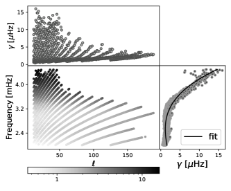
We choose a simplified model of the damping $\gamma$ by fitting a third-order polynomial in frequency to the measured seismic line-widths obtained from the $72$-day MDI mode-parameter set (Schou, 1999), plotted in Figure 1. We use Model S (Christensen-Dalsgaard et al., 1996) to obtain the structure parameters.

Figure 1: Model capturing seismic wave attenuation in the Sun. The solid line in the lower right panel represents a cubic-polynomial fit to the frequency variation of the line-width.

Waves propagating in the frequency channel $\nu=\omega/2\pi$ from source location $\mathbf{x}_{\text{src}}$ to the observation point $\mathbf{x}$ may equivalently be described by the Green function $\mathbf{G}\left(\mathbf{x},\mathbf{x}_{\text{src}},\omega\right)$ corresponding to the wave operator $\mathcal{L}$. The Green function in this case is a rank-$2$ tensor that satisfies

$$\mathcal{L}\mathbf{G}\left(\mathbf{x},\mathbf{x}_{\text{src}},\omega\right)=\delta\left(\mathbf{x}-\mathbf{x}_{\text{src}}\right)\mathbf{I},$$ (9)

where $\mathbf{I}$ is the $3\times 3$ identity matrix. The Green function $\mathbf{G}$ has nine components that relate the three vector components of the source $\mathbf{S}$ to those of the displacement $\bm{\xi}$,

$$\xi_{i}\left(\mathbf{x},\omega\right)=\int d\mathbf{x}_{\text{src}}G_{ij}\left(\mathbf{x},\mathbf{x}_{\text{src}},\omega\right)S_{j}\left(\mathbf{x}_{\text{src}},\omega\right).$$ (10)

The fact that eigenfunctions of the wave operator $\mathcal{L}$ are strictly spheroidal implies that the Green function may be expanded in terms of $\mathbf{Y}_{jm}^{\left(-1\right)}$ and $\mathbf{Y}_{jm}^{\left(+1\right)}$, and that only four of the nine components of the Green function are independent — the ones that relate the spheroidal component of the sources to those of the displacement. We use the fact that the Green function may be expressed as an outer product of the eigenfunctions. This suggests a natural expansion of the the Green function in the Hansen VSH basis as

$$\mathbf{G}\left(\mathbf{x}_{\text{obs}},\mathbf{x}_{\text{src}};\omega\right)= \sum_{\alpha,\beta=\pm 1}\sum_{jm}G_{\left(\beta\right),j\omega}^{\left(\alpha\right)}\left(r_{\text{obs}},r_{\text{src}}\right)\times$$

$$\mathbf{Y}_{jm}^{\left(\alpha\right)}\left(\hat{n}_{\text{obs}}\right)\mathbf{Y}_{jm}^{\left(\beta\right)*}\left(\hat{n}_{\text{src}}\right),$$ (11)

where the component $G_{\left(\beta\right),j\omega}^{\left(\alpha\right)}\left(r_{\text{obs}},r_{\text{src}}\right)$ relates the source component $S_{jm}^{\left(\beta\right)}\left(r_{\text{src}}\right)$ to the displacement component $\xi_{jm}^{\left(\alpha\right)}\left(r_{\text{obs}}\right)$ that is measured at the point $\mathbf{x}_{\text{obs}}$. The placement of Greek indices in the super and subscripts, i.e. $G_{\left(\beta\right),j\omega}^{\left(\alpha\right)}$, indicates that the Green function is a mixed tensor, something that might be verified by noting that $\mathbf{Y}_{jm}^{\left(\beta\right)*}=\mathbf{Y}_{jm}^{\left(\beta\right)\dagger}$ is a contravariant basis vector whereas $\mathbf{Y}_{jm}^{\left(\alpha\right)}$ is a covariant one. The radius $r_{\text{obs}}$ may be thought of as a representative height that arises from the Dopplergram response function convolved with the line-formation heights. An accurate estimate of the observation height might be necessary for a consistent interpretation of seismic travel-times, including its center-to-limb variation (Wachter, 2008; Fleck et al., 2011; Kitiashvili et al., 2015).

We compute the radial components of the Green function using a high-order finite-difference approximation to Equation (9) following Mandal et al. (2017). We detail the analysis in Appendix A. The computation of line-of-sight projected measurements is easier in the basis of the PB VSH owing to the fact that these are diagonal in the helicity basis. We express the Green function as

$$\mathbf{G}\left(\mathbf{x}_{\text{obs}},\mathbf{x}_{\text{src}};\omega\right)= \sum_{\alpha,\beta=-1}^{1}\sum_{jm}G_{\beta,j\omega}^{\alpha}\left(r_{\text{obs}},r_{\text{src}}\right)\times$$

$$\mathbf{Y}_{jm}^{\alpha}\left(\hat{n}_{\text{obs}}\right)\mathbf{Y}_{jm}^{\beta*}\left(\hat{n}_{\text{src}}\right),$$ (12)

where the independent components of the Green function are related to those in the Hansen basis through

$$G_{0,j\omega}^{0} =G_{\left(-1\right),j\omega}^{\left(-1\right)},\quad G_{0,j\omega}^{+}=\frac{1}{\sqrt{2}}G_{\left(-1\right),j\omega}^{\left(1\right)},$$ (13)

$$G_{+,j\omega}^{0} =\frac{1}{\sqrt{2}}G_{\left(1\right),j\omega}^{\left(-1\right)},\quad G_{+,j\omega}^{+}=\frac{1}{2}G_{\left(1\right),j\omega}^{\left(1\right)},$$

The choice of independent $\alpha$ and $\beta$ in the PB VSH basis is arbitrary, and we may choose to retain any four independent components from Equation (A16).

3.1 Change in Green function

We choose to look at small-amplitude time-invariant perturbations in the sound speed $c\left(\mathbf{x}\right)$, where $\mathbf{x}$ ranges over all spatial locations within the Sun where the sound speed is finite. A local change in the sound speed — denoted by by $\delta c\left(\mathbf{x}\right)$ — leads to a change in the wave operator by the amount $\delta\mathcal{L}=-2\bm{\nabla}\left(\rho c\delta c\bm{\nabla}\cdot\right)$ to the linear order. A change in the wave operator by $\delta\mathcal{L}$ leads to a corresponding change in the Green function that may be computed in the First Born approximation as

$$\delta\mathbf{G}\left(\mathbf{x}_{\text{obs}},\mathbf{x}_{\text{src}},\omega\right)=-\int d\mathbf{x}\,\mathbf{G}\left(\mathbf{x}_{\text{obs}},\mathbf{x},\omega\right)\cdot\delta\mathcal{L}\mathbf{G}\left(\mathbf{x},\mathbf{x}_{\text{src}},\omega\right).$$ (14)

We substitute $\delta\mathcal{L}=-2\bm{\nabla}\left(\rho c\delta c\bm{\nabla}\cdot\right)$ into Equation (14) and integrate by parts using Gauss’ divergence theorem. We assume zero-Dirichlet boundary conditions in radius and therefore drop the boundary term, and use the seismic reciprocity relation $\mathbf{G}^{T}\left(\mathbf{x}_{1},\mathbf{x}_{2}\right)=\mathbf{G}\left(\mathbf{x}_{2},\mathbf{x}_{1}\right)$, where the tensor transpose is defined as ${\bf G}^{T}_{ij}={\bf G}_{ji}$, to obtain

$$\delta\mathbf{G}\left(\mathbf{x}_{\text{obs}},\mathbf{x}_{\text{src}},\omega\right)=-2\int d\mathbf{x}\,\rho c\,\bm{\nabla}\cdot\mathbf{G}\left(\mathbf{x},\mathbf{x}_{\text{obs}},\omega\right)\bm{\nabla}\cdot\mathbf{G}\left(\mathbf{x},\mathbf{x}_{\text{src}},\omega\right)\delta c\left(\mathbf{x}\right).$$ (15)

We have not explored the ramifications of including transparent boundary conditions as used by Gizon et al. (2017), which lets high-frequency waves (above the acoustic cutoff of $5.5\,\text{mHz}$) leak out, and is expected to be a more realistic representation of the conditions that exist on the Sun (see e. g. Kumar et al., 1990).

The perturbation $\delta c\left(\mathbf{x}\right)$ is a scalar field, and it may be expanded in the basis of spherical harmonics as

$$\delta c\left(\mathbf{x}\right)=\sum_{\ell m}\delta c_{\ell m}\left(r\right)Y_{\ell m}\left(\hat{n}\right).$$ (16)

Since $\delta c\left(\mathbf{x}\right)$ is real, the spherical harmonic components $\delta c_{\ell m}\left(r\right)$ satisfy $\delta c_{\ell,-m}\left(r\right)=\left(-1\right)^{m}\delta c_{\ell m}^{*}\left(r\right)$ and therefore the components for $m\geq 0$ suffice to completely describe the spatial variation. We seek to express Equation (15) in terms of the components $\delta c_{\ell m}\left(r\right)$. We note that the divergence of the Green function may be evaluated in the PB VSH basis (see Dahlen & Tromp, 1998) to

$$\bm{\nabla}\cdot\mathbf{G}\left(\mathbf{x},\mathbf{x}_{i};\omega\right)=\sum_{jm\beta}\left[\bm{\nabla}\cdot\mathbf{G}\right]_{\beta j\omega}\left(r,r_{i}\right)Y_{jm}\left(\hat{n}\right)\mathbf{Y}_{jm}^{\beta*}\left(\hat{n}_{i}\right),$$ (17)

where $\left[\bm{\nabla}\cdot\mathbf{G}\right]_{\beta j\omega}\left(r,r_{i}\right)$ is the radial profile of the divergence of $\mathbf{G}$ for a source directed along $\mathbf{Y}_{jm}^{\beta}\left(\hat{n}_{i}\right)$, and is related to the components of the Green function through

$$\left[\bm{\nabla}\cdot\mathbf{G}\right]_{\beta j\omega}\left(r,r_{i}\right)= -\frac{\sqrt{2j\left(j+1\right)}}{r}G_{\beta,j\omega}^{1}\left(r,r_{i}\right)+$$

$$\left(\frac{d}{dr}+\frac{2}{r}\right)G_{\beta,j\omega}^{0}\left(r,r_{i}\right).$$ (18)

Substituting Equations (16) and (17) into Equation (15) and integrating over the scattering angle $\hat{n}$, we obtain

$$\delta\mathbf{G}\left(\mathbf{x}_{\text{obs}},\mathbf{x}_{\text{src}},\omega\right) =-2\int r^{2}dr\,\rho c\sum_{\ell m}\delta c_{\ell m}\left(r\right)\times$$

$$\sum_{\beta_{1},\beta_{2}=\pm 1}\sum_{j_{1}m_{1}}\sum_{j_{2}m_{2}}\left[\bm{\nabla}\cdot\mathbf{G}\right]_{\beta_{1}j_{1}\omega}\left(r,r_{\text{obs}}\right)\times$$

$$\left[\bm{\nabla}\cdot\mathbf{G}\right]_{\beta_{2}j_{2}\omega}\left(r,r_{\text{src}}\right)\times$$

$$\sqrt{\frac{\left(2j_{1}+1\right)\left(2j_{2}+1\right)\left(2\ell+1\right)}{4\pi}}\times$$

$$\left(\begin{array}[]{ccc}j_{1}&j_{2}&\ell\\ 0&0&0\end{array}\right)\left(\begin{array}[]{ccc}j_{1}&j_{2}&\ell\\ m_{1}&m_{2}&m\end{array}\right)\times$$ (23)

$$\mathbf{Y}_{j_{1}m_{1}}^{\beta_{1}*}\left(\hat{n}_{\text{obs}}\right)\mathbf{Y}_{j_{2}m_{2}}^{\beta_{2}*}\left(\hat{n}_{\text{src}}\right),$$ (24)

where the angular degrees $j_{1}$, $j_{2}$ and $\ell$ are related by the triangle constraint $\left|j_{1}-j_{2}\right|\leq\ell\leq j_{1}+j_{2}$, and the Wigner $3$-j symbols are non-zero only for $m_{1}+m_{2}+m=0$. For a particular choice of $\ell$, we choose $j_{1}$ to vary independently, which would constrain $j_{2}$ to the range $\left|j_{1}-\ell\right|\leq j_{2}\leq j_{1}+\ell$. We may also choose $m_{1}$ to vary independently for a particular choice of $m$, which would peg $m_{2}$ to $m-m_{1}$. This reduces the number of terms contributing to Equation (24) significantly. In subsequent analysis, we use Clebsch-Gordan coefficients instead of the Wigner $3$-j symbols, the two being related through

$$C_{j_{1}m_{1}j_{2}m_{2}}^{\ell m}=\left(-1\right)^{j_{1}-j_{2}+m}\sqrt{2\ell+1}\left(\begin{array}[]{ccc}j_{1}&j_{2}&\ell\\ m_{1}&m_{2}&-m\end{array}\right).$$

The motivation for this switch is that we use bipolar spherical harmonics, and Clebsch-Gordan coefficients are the matrix elements corresponding to the transformation between the bipolar and the product of monopolar harmonics.

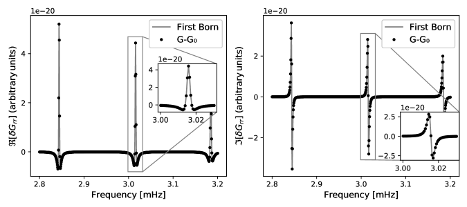
We verify Equation (24) by comparing the radial component of $\delta\mathbf{G}$ for an isotropic sound-speed perturbation $\delta c\left(r\right)$ with that computed from the difference in the full Green functions. A spherically symmetric perturbation $\delta c\left(r\right)$ may be expanded in a basis of spherical harmonics in terms of only the component corresponding to $\ell=0$ and $m=0$ as $\delta c\left(r\right)=\delta c_{00}\left(r\right)/\sqrt{4\pi}$. The imposition of $\ell=0$ necessitates $j_{2}=j_{1}$, and $m=0$ implies $m_{1}=-m_{2}$. Limiting the sum in Equation (24) to only the non-zero terms, we obtain the expression for the radial component to be

$$\delta G_{rr}\left(\mathbf{x}_{\text{obs}},\mathbf{x}_{\text{src}},\omega\right)= -2\int r^{2}dr\,\rho\,c\,\delta c\,\left(r\right)\times$$

$$\sum_{j}\frac{\left(2j+1\right)}{4\pi}\left[\bm{\nabla}\cdot\mathbf{G}\right]_{0j\omega}\left(r,r_{\text{obs}}\right)\times$$

$$\left[\bm{\nabla}\cdot\mathbf{G}\right]_{0j\omega}\left(r,r_{\text{src}}\right)P_{j}\left(\hat{n}_{\text{obs}}\cdot\hat{n}_{\text{src}}\right).$$ (25)

Similar to Mandal et al. (2017), we choose $\delta c\left(r\right)=10^{-5}c\left(r\right)$ and compute $\delta G_{rr}\left(\mathbf{x}_{\text{obs}},\mathbf{x}_{\text{src}},\omega\right)$ from Equation (25). Alternately such a perturbation may be interpreted as a change in the radial profile of the background sound speed, so we evaluate the Green functions following the prescription in Section 3 for the original and altered sound-speed profiles. We compute $\delta G_{rr,\delta c}$ as $G_{rr,c+\delta c}\left(\mathbf{x}_{\text{obs}},\mathbf{x}_{\text{src}},\omega\right)-G_{rr,c}\left(\mathbf{x}_{\text{obs}},\mathbf{x}_{\text{src}},\omega\right)$, where the subscript indicates the sound-speed profile that is used in the background model. We plot both these functions in Figure 2. The close match between the result in the VSH basis and that obtained in the spherical polar basis serves to validate the formalism used in this work.

Figure 2: Change in the radial component of the Green function ($\delta G_{rr}$) for an isotropic perturbation in sound speed, computed using the first Born approximation (line) and as the difference between the Green functions in the two models (dots). The left panel shows the real part of $\delta G_{rr}$ and the right one shows the imaginary component. The Green function has been computed for $\ell=40$, and only a section of the frequency range has been displayed.

4 Cross-covariance

Waves in the Sun are generated stochastically by sources located all over the solar surface. Therefore, to model this behaviour, we study the expected cross-covariance $C\left(\mathbf{x}_{1},\mathbf{x}_{2},\omega\right)$ between line-of-sight projected Doppler wave velocities measured at points $\mathbf{x}_{1}$ and $\mathbf{x}_{2}$ on the solar surface. This quantity is obtained by ensemble averaging over many stochastic source distributions. We denote the line-of-sight vector at the point $\mathbf{x}_{i}$ on the solar surface by $\bm{l}\left(\hat{n}_{i}\right)$. We express the cross-covariance in temporal frequency domain as

$$C\left(\mathbf{x}_{1},\mathbf{x}_{2};\omega\right)=\omega^{2}\left\langle\bm{l}\left(\mathbf{x}_{1}\right)\cdot\bm{\xi}^{*}\left(\mathbf{x}_{1};\omega\right)\bm{l}\left(\mathbf{x}_{2}\right)\cdot\bm{\xi}\left(\mathbf{x}_{2};\omega\right)\right\rangle,$$ (26)

where $\bm{l}\left(\mathbf{x}_{i}\right)$ is the line-of-sight vector from the point $\mathbf{x}_{i}$ on the Sun directed towards the detector, $\bm{\xi}\left(\mathbf{x};\omega\right)$ is the wave displacement, and the angular brackets denote an ensemble average. Our results may be compared to that obtained by Böning et al. (2016) by setting $\bm{l}\left(\mathbf{x}_{i}\right)=\mathbf{e}_{r}$, and we refer to this as the radial approximation henceforth. We note that the line-of-sight projection breaks the spherical symmetry inherent to the system, since the line-of-sight is computed with respect to a detector fixed in space. This issue is skirted in the radial assumption, in which case, the measured cross-covariance is independent of the detector location and depends only on the angular distance between the observation points.

Seismic wave displacements are related to the sources exciting them through the Green function in Equation (10). Following Böning et al. (2016), we assume that the wave source $\mathbf{S}\left(\mathbf{x};\omega\right)$ may be represented as a realization of a stationary stochastic process having a covariance

$$\left\langle S_{i}^{*}\left(\mathbf{x}_{1};\omega\right)S_{j}\left(\mathbf{x}_{2};\omega\right)\right\rangle=P\left(\omega\right)\delta\left(\mathbf{x}_{1}-\mathbf{x}_{2}\right)\delta_{ir}\delta_{jr}\times\frac{1}{r_{\text{src}}^{2}}\delta\left(\left|\mathbf{x}_{1}\right|-r_{\text{src}}\right),$$ (27)

where $P\left(\omega\right)$ is the power spectrum of the sources, and $r_{\text{src}}$ is the radial coordinate at which seismic waves are excited. This model of the source covariance is inspired by the observation that much of the non-adiabatic pressure fluctuations that excite sound waves in the Sun take place in a thin layer of about a few hundred kilometers below the photosphere, and the fluctuations occur predominantly in filamentary downdrafts (Stein & Nordlund, 1989; Nordlund & Stein, 1991). A better model of the covariance might be obtained from numerical simulations of near-surface layers in the Sun, although we do not explore such an approach in the present work.

In this approximation, we simplify Equation (26) to obtain

$$C\left(\mathbf{x}_{1},\mathbf{x}_{2};\omega\right)=\omega^{2}P\left(\omega\right)\int d\Omega_{\text{src}}\,\bm{l}\left(\mathbf{x}_{1}\right)\cdot\mathbf{G}_{r}^{*}\left(\mathbf{x}_{1},\mathbf{x}_{\text{src}};\omega\right)\bm{l}\left(\mathbf{x}_{2}\right)\cdot\mathbf{G}_{r}\left(\mathbf{x}_{2},\mathbf{x}_{\text{src}};\omega\right),$$ (28)

where $\mathbf{G}_{r}\left(\mathbf{x}_{i},\mathbf{x}_{\text{src}};\omega\right)=\mathbf{G}\left(\mathbf{x}_{i},\mathbf{x}_{\text{src}};\omega\right)\cdot\hat{n}_{\text{src}}$ is the Green vector corresponding to a radial source, and the integral is carried out over the angular distribution of sources in the Sun. We carry out the integral to obtain

$$C\left(\mathbf{x}_{1},\mathbf{x}_{2};\omega\right)=\omega^{2}P\left(\omega\right)\sum_{\alpha,\beta=-1}^{1}\sum_{jm}G_{0,j\omega}^{\alpha*}\left(r_{1},r_{\text{src}}\right)G_{0,j\omega}^{\beta}\left(r_{2},r_{\text{src}}\right)\bm{l}\left(\mathbf{x}_{1}\right)\cdot\mathbf{Y}_{jm}^{\alpha*}\left(\hat{n}_{1}\right)\bm{l}\left(\mathbf{x}_{2}\right)\cdot\mathbf{Y}_{jm}^{\beta}\left(\hat{n}_{2}\right).$$ (29)

We introduce the line-of-sight projected bipolar vector spherical harmonic

$$Y_{\ell m}^{j_{1}j_{2},\alpha\beta}\left(\mathbf{x}_{\text{1}},\mathbf{x}_{2}\right)=\sum_{m_{1}m_{2}}C_{j_{1}m_{1}j_{2}m_{2}}^{\ell m}\bm{l}\left(\mathbf{x}_{\text{1}}\right)\cdot\mathbf{Y}_{j_{1}m_{1}}^{\alpha}\left(\hat{n}_{\text{1}}\right)\bm{l}\left(\mathbf{x}_{2}\right)\cdot\mathbf{Y}_{j_{2}m_{2}}^{\beta}\left(\hat{n}_{2}\right),$$ (30)

and rewrite Equation (29) in a concise notation as

$$C\left(\mathbf{x}_{1},\mathbf{x}_{2};\omega\right)=\omega^{2}P\left(\omega\right)\sum_{\alpha,\beta=-1}^{1}\sum_{j}\left(-1\right)^{j}\sqrt{2j+1}G_{0,j\omega}^{\alpha*}\left(r_{1},r_{\text{src}}\right)G_{0,j\omega}^{\beta}\left(r_{2},r_{\text{src}}\right)Y_{00}^{jj,\alpha\beta}\left(\mathbf{x}_{\text{1}},\mathbf{x}_{2}\right).$$ (31)

The bipolar function $Y_{\ell m}^{j_{1}j_{2},\alpha\beta}\left(\mathbf{x}_{\text{1}},\mathbf{x}_{2}\right)$ does not transform as a spherical tensor under rotation in general, as the line-of-sight projection explicitly breaks the spherical symmetry. In the radial assumption, we set $\bm{l}\left(\mathbf{x}_{i}\right)=\mathbf{e}_{r}$ and obtain $Y_{\ell m}^{j_{1}j_{2},\alpha\beta}\left(\mathbf{x}_{\text{1}},\mathbf{x}_{2}\right)=Y_{\ell m}^{j_{1}j_{2},00}\left(\mathbf{x}_{\text{1}},\mathbf{x}_{2}\right)=Y_{j_{1}j_{2}}^{\ell m}\left(\hat{n}_{\text{1}},\hat{n}_{2}\right)$, which is the ordinary bipolar spherical harmonic and transforms as a spherical tensor. We have chosen the notation to denote the parallel with bipolar spherical harmonics. In particular, the function $Y_{\ell m}^{j_{1}j_{2},\alpha\beta}\left(\mathbf{x}_{\text{1}},\mathbf{x}_{2}\right)$ may be written as

$$Y_{\ell m}^{j_{1}j_{2},\alpha\beta}\left(\mathbf{x}_{\text{1}},\mathbf{x}_{2}\right)=\left[\bm{l}\left(\mathbf{x}_{\text{1}}\right)\bm{l}\left(\mathbf{x}_{2}\right)\right]:\mathbf{Y}_{\ell m}^{j_{1}j_{2},\alpha\beta}\left(\hat{n}_{1},\hat{n}_{2}\right),$$

where the colon denotes a double contraction $\left(\mathbf{A}:\mathbf{B}=A_{ij}\,B_{ij}\right)$, and $\mathbf{Y}_{\ell m}^{j_{1}j_{2},\alpha\beta}\left(\hat{n}_{1},\hat{n}_{2}\right)$ is a bipolar vector spherical harmonic. This allows us to separate out the transformation under rotation into two parts, one for the bipolar harmonic and one for the line-of-sight tensor. The rotation matrix for the former is the Wigner D-matrix, whereas the latter may be evaluated by explicitly evaluating the line-of-sight vectors at the two points. The analysis is simplified in the radial approximation where the line-of-sight tensor $\mathbf{e}_{r}\mathbf{e}_{r}$ does not change its form on rotations.

As a sanity check, we look at the scenario where the line-of-sight is assumed to be radial at both the observation points, which, in our notation, implies retaining only the term corresponding to $\alpha=\beta=0$ in Equation (31). The angular term $Y_{00}^{jj,00}\left(\mathbf{x}_{\text{1}},\mathbf{x}_{2}\right)$ reduces to the bipolar spherical harmonic $Y_{00}^{jj}\left(\hat{n}_{1},\hat{n}_{2}\right)$ in this approximation. We use $Y_{00}^{jj}\left(\hat{n}_{\text{1}},\hat{n}_{2}\right)=\left(-1\right)^{j}\sqrt{2j+1}P_{j}\left(\hat{n}_{\text{1}}\cdot\hat{n}_{2}\right)/4\pi$ — where $P_{j}$ is the Legendre polynomial of degree $j$ — to obtain

$$C_{r}\left(\mathbf{x}_{1},\mathbf{x}_{2};\omega\right)=\omega^{2}P\left(\omega\right)\sum_{j}\frac{\left(2j+1\right)}{4\pi}G_{0,j\omega}^{0*}\left(r_{1},r_{\text{src}}\right)G_{0,j\omega}^{0}\left(r_{2},r_{\text{src}}\right)P_{j}\left(\hat{n}_{\text{1}}\cdot\hat{n}_{2}\right).$$ (32)

In the PB VSH basis, $G_{0,j\omega}^{0}=G_{rr,j\omega}$. The expression in Equation (32) is precisely the result that we expect if we choose to compute the cross-covariance between the radial components of the displacement. The other combinations of $\alpha$ and $\beta$ in Equation (31) arise as projections of the tangential wave components in the direction of the line-of-sight.

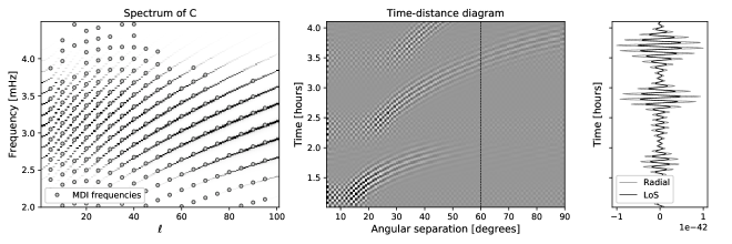
We plot the time-domain cross-covariances in Figure 3 for one observation point on the equator at $\phi=0$ at a height of $200\,\text{km}$ above the photosphere, and the second point at various different azimuths on the equator and at the same observation height, assuming a Gaussian $P\left(\omega\right)$ with a mean of $2\pi\times 3\,\text{mHz}$ and a width of $2\pi\times 0.4\,\text{mHz}$. We choose this functional form for the temporal spectrum $P\left(\omega\right)$ in numerical evaluations subsequently in the analysis.

Figure 3: Left panel: Spectrum of the cross-covariance of radial components of wave displacement, overlain with selected mode frequencies obtained from the MDI pipeline (Schou, 1999). Middle panel: Time-distance diagram obtained for the radial component of the displacement. Right panel: The cross-covariance between two points on the equator at $\phi=0$ and $\phi=60$, computed using the radial components of the displacement (grey) and the line-of-sight projected component of the displacement (black).

4.1 Change in cross-covariance

A local change in the background sound speed by $\delta c\left(\mathbf{x}\right)$ would alter the Green function by an amount $\delta\mathbf{G}$ that is described by Equation (24). The change in the Green function will lead to a corresponding variation in the measured wave fields at the two observation points, and subsequently to a difference in the cross covariance. We may express this change as

$$\delta C\left(\mathbf{x}_{1},\mathbf{x}_{2};\omega\right)=\omega^{2}P\left(\omega\right)\int d\Omega_{\text{src}}\,\left[\bm{l}\left(\mathbf{x}_{1}\right)\cdot\delta\mathbf{G}_{r}^{*}\left(\mathbf{x}_{1},\mathbf{x}_{\text{src}};\omega\right)\bm{l}\left(\mathbf{x}_{2}\right)\cdot\mathbf{G}_{r}\left(\mathbf{x}_{2},\mathbf{x}_{\text{src}};\omega\right)\right.$$

$$\left.+\bm{l}\left(\mathbf{x}_{1}\right)\cdot\mathbf{G}_{r}^{*}\left(\mathbf{x}_{1},\mathbf{x}_{\text{src}};\omega\right)\bm{l}\left(\mathbf{x}_{2}\right)\cdot\delta\mathbf{G}_{r}\left(\mathbf{x}_{2},\mathbf{x}_{\text{src}};\omega\right)\right],$$ (33)

where $\delta\mathbf{G}$ is given by Equation (24). We compute the change in the cross covariance in terms of the spherical-harmonic coefficients of the sound-speed perturbation,

$$\delta C\left(\mathbf{x}_{1},\mathbf{x}_{2};\omega\right)= \omega^{2}P\left(\omega\right)\sum_{\ell m}\int r^{2}dr\delta c_{\ell m}\left(r\right)\sum_{\delta\left(j_{1}j_{2},\ell\right)}N_{j_{1}j_{2}\ell}$$

$$\sum_{\alpha\beta}T_{\alpha,j_{1}j_{2}\omega}^{\beta}\left(r,r_{1},r_{2},r_{\text{src}}\right)Y_{\ell m}^{j_{1}j_{2},\alpha\beta}\left(\mathbf{x}_{1},\mathbf{x}_{2}\right),$$ (34)

where the terms $N_{j_{1}j_{2}\ell}$ and $T_{\alpha,j_{1}j_{2}\omega}^{\beta}$ are defined as

$$N_{j_{1}j_{2}\ell}= \sqrt{\frac{\left(2j_{1}+1\right)\left(2j_{2}+1\right)}{4\pi\left(2\ell+1\right)}}C_{j_{1}0j_{2}0}^{\ell 0},$$ (35)

$$T_{\alpha,j_{1}j_{2}\omega}^{\beta}\left(r,r_{1},r_{2},r_{\text{src}}\right)= H_{\alpha,j_{1}j_{2}\omega}^{\beta}\left(r,r_{1},r_{2},r_{\text{src}}\right)+$$

$$H_{\beta,j_{2}j_{1}\omega}^{\alpha*}\left(r,r_{2},r_{1},r_{\text{src}}\right),$$ (36)

$$H_{\alpha,j_{1}j_{2}\omega}^{\beta}\left(r,r_{1},r_{2},r_{\text{src}}\right)= -2\rho c\left[\bm{\nabla}\cdot\mathbf{G}\right]_{\alpha,j_{1}\omega}^{*}\left(r,r_{1}\right)\times$$

$$\left[\bm{\nabla}\cdot\mathbf{G}\right]_{0,j_{2}\omega}^{*}\left(r,r_{\text{src}}\right)\times$$

$$G_{0,j_{2}\omega}^{\beta}\left(r_{2},r_{\text{src}}\right),$$ (37)

and $\delta\left(j_{1}j_{2},\ell\right)$ as a summation index indicates a sum over all whole-number values of $j_{1}$ and $j_{2}$ that are related to $\ell$ through the triangle inequality $\left|j_{1}-\ell\right|\leq j_{2}\leq j_{1}+\ell$. We note that $C_{j_{1}0j_{2}0}^{\ell 0}$ is non-zero only if $j_{1}+j_{2}+\ell$ is even, which implies that contributions towards sound-speed modes with odd-$\ell$ come only from wave-mode pairs $\left(j_{1},j_{2}\right)$ for which $j_{1}+j_{2}$ is odd, and similarly for even ones. This limits the number of terms that contribute to the summation in Equation (34).

An isotropic sound-speed perturbation $\delta c\left(r\right)$ would lead to the angular variation being described by $Y_{00}^{j_{1}j_{2},\alpha\beta}\left(\mathbf{x}_{\text{1}},\mathbf{x}_{2}\right).$ We recognize that this term has the same angular variation as the cross-covariance from Equation (31). This is consistent with the idea that a radial perturbation $\delta c\left(r\right)$ changes the background sound speed from $c\left(r\right)$ to $c\left(r\right)+\delta c\left(r\right)$ while still preserving spherical symmetry of the medium, and we may therefore evaluate the change in cross covariance directly as the difference in the cross covariances computed in each model.

4.2 Numerical evaluation of change in cross-covariance

We use the publicly available library SHTOOLS (Wieczorek & Meschede, 2018) to compute the Clebsch-Gordan coefficients that enter Equations (30) and (35). The library can produce reliable estimates of Clebsch Gordan coefficients till an angular degree of around $160$. We compute the PB VSH using the fact that the generalized spherical harmonics $Y_{jm}^{\alpha}$ may be computed as phase-shifted elements of the Wigner d-matrix $d_{-\alpha-m}^{j}$. We compute the Wigner d-matrix elements through an exact diagonalization of the angular momentum operator $J_{y}$ following the prescription laid out by Feng et al. (2015). This produces Wigner d-matrices with an accuracy of $10^{-14}$ for $j\leq 100$. We therefore limit ourselves to $j_{1},j_{2}\leq 80$ in this work, so that by the triangle inequality we obtain $\ell\leq j_{1}+j_{2}\leq 160$. Assuming a radial line-of-sight reduces the generalized spherical harmonics $Y_{jm}^{\alpha}$ to regular spherical harmonics $Y_{jm}$ which may be computed accurately till much higher orders, for example with absolute or relative errors $\leq 10^{-10}$ up to $j\sim 1000$ using the recursive algorithm prescribed by Limpanuparb & Milthorpe (2014).

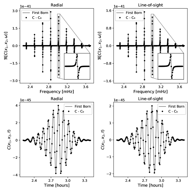
We verify our result by using an isotropic sound-speed perturbation $\delta c\left(r\right)=\delta c_{00}\left(r\right)/\sqrt{4\pi}$. An isotropic sound-speed perturbation may be interpreted as a change in the background sound speed profile to $c\left(r\right)+\delta c\left(r\right)$, and we may compute the cross covariance in this model using Equation (28). We choose a specific model of the perturbation given by $\delta c\left(r\right)=10^{-5}c\left(r\right)$. We compute $\delta C_{\delta c}\left(\mathbf{x}_{1},\mathbf{x}_{2};\omega\right)=C_{c+\delta c}\left(\mathbf{x}_{1},\mathbf{x}_{2};\omega\right)-C_{c}\left(\mathbf{x}_{1},\mathbf{x}_{2};\omega\right)$ — where the subscript indicates the sound-speed profile in the background model — and compare it with

$$\delta C\left(\mathbf{x}_{1},\mathbf{x}_{2};\omega\right)\,=\, \omega^{2}P\left(\omega\right)\int r^{2}dr\delta c\left(r\right)\sum_{j}\left(-1\right)^{j}\sqrt{2j+1}\sum_{\alpha,\beta=-1}^{1}T_{\alpha,jj\omega}^{\beta}\left(r,r_{1},r_{2},r_{\text{src}}\right)Y_{00}^{jj,\alpha\beta}\left(\mathbf{x}_{1},\mathbf{x}_{2}\right).$$ (38)

We plot the two functions in Figure 4. We also compare the change in cross-covariances using only the radial components. We find that the significant difference introduced by the projection is in the amplitude of the change in cross-covariance.

Figure 4: Change in cross-covariance computed using the first Born approximation (solid gray line) and as the direct difference between the cross covariances computed using two different models of radial sound-speed profiles. The top row represents $\delta C$ in frequency domain for $\ell=40$, whereas the bottom row represents the $\delta C$ in time domain, computed by summing over all modes lying in $5\leq\ell\leq 80$. The left panel is computed using the radial components of wave displacement, whereas the right panel is computed using the line-of-sight projected components.

5 Sensitivity kernel

5.1 Travel time

A change in propagation speeds would leave its imprint on the time taken by waves to travel between two points on the Sun. An estimate of this change may be determined by following Gizon & Birch (2002) as

$$\delta\tau\left(\mathbf{x}_{1},\mathbf{x}_{2}\right)=\int_{0}^{\infty}\frac{d\omega}{2\pi}\,2\Re\left[h^{*}\left(\mathbf{x}_{1},\mathbf{x}_{2},\omega\right)\delta C\left(\mathbf{x}_{1},\mathbf{x}_{2},\omega\right)\right],$$ (39)

where $h\left(\mathbf{x}_{1},\mathbf{x}_{2},\omega\right)$ is a weighing function that depends on the specific measurement technique and is computed in terms of the cross-covariance $C\left(\mathbf{x}_{1},\mathbf{x}_{2},\omega\right)$. We may use Equation (34) to recast Equation (39) in the form

$$\delta\tau\left(\mathbf{x}_{1},\mathbf{x}_{2}\right)=\sum_{\ell m}\int_{0}^{R\odot}dr\,r^{2}K_{\ell m}^{*}\left(r,\mathbf{x}_{1},\mathbf{x}_{2}\right)\delta c_{\ell m}\left(r\right),$$ (40)

where the kernel components $K_{\ell m}\left(r,\mathbf{x}_{1},\mathbf{x}_{2}\right)$ are given by

$$K_{\ell m}\left(r,\mathbf{x}_{1},\mathbf{x}_{2}\right)=\int_{0}^{\infty}\frac{d\omega}{2\pi}\,\omega^{2}P\left(\omega\right)\,\sum_{\delta\left(j_{1}j_{2},\ell\right)}\sum_{\alpha\beta}N_{j_{1}j_{2}\ell}\,2\Re\left[h^{*}\left(\mathbf{x}_{1},\mathbf{x}_{2},\omega\right)T_{\alpha,j_{1}j_{2}\omega}^{\beta}\left(r,r_{1},r_{2},r_{\text{src}}\right)\right]Y_{\ell m}^{j_{1}j_{2},\alpha\beta*}\left(\mathbf{x}_{1},\mathbf{x}_{2}\right).$$ (41)

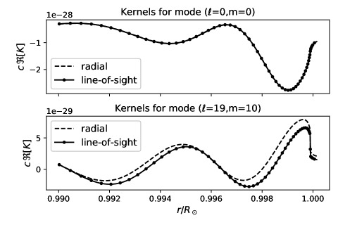
Equation (40) sets up an inverse problem for the sound-speed perturbation in terms of the measured travel times $\delta\tau\left(\mathbf{x}_{1},\mathbf{x}_{2}\right)$, where the kernel incorporates the effect of line-of-sight projection and variation in the center-to-limb observational heights. We plot the radial profile of the kernel for various $\left(\ell,m\right)$ pairs in Figure 5 in the radial line-of-sight approximation, choosing two observation points located at a co-latitude of $45$ degrees, and having azimuths of $-45$ degrees and $45$ degrees respectively. We need only compute $K_{\ell m}$ for $m\geq 0$ in the inverse problem in Equation (40), as $\delta c\left(\mathbf{x}\right)$ is a real function in space.

Figure 5: Profiles of kernel components for modes $(\ell=0,m=0)$ (top) and $(\ell=19,m=10)$ (bottom), computed using radial and line-of-sight projected wave displacements.

We may construct the three-dimensional kernel $K\left(\mathbf{x},\mathbf{x}_{1},\mathbf{x}_{2}\right)$ by summing over spherical harmonics as

$$K\left(\mathbf{x},\mathbf{x}_{1},\mathbf{x}_{2}\right)=\sum_{\ell m}K_{\ell m}\left(r,\mathbf{x}_{1},\mathbf{x}_{2}\right)Y_{\ell m}\left(\theta,\phi\right).$$ (42)

The inverse problem in Equation (40) is $1.5$-dimensional, and does not require a computation of the three-dimensional kernel.

5.2 Validating the travel-time kernel: radial displacements

We verify that the analysis produces the expected result by matching the expression for the kernel in Equation (41) with that obtained by carrying out a spherical harmonic decomposition of the three-dimensional fleshed-out kernel. We start by computing the cross-covariance of the radial component of the displacement measured at two points. The corresponding three-dimensional travel-time kernel evaluates to

$$K\left(\mathbf{x},\mathbf{x}_{1},\mathbf{x}_{2}\right)= \int_{0}^{\infty}\frac{d\omega}{2\pi}\,\omega^{2}P\left(\omega\right)\sum_{j_{1}j_{2}}\frac{\left(2j_{1}+1\right)}{4\pi}\frac{\left(2j_{2}+1\right)}{4\pi}P_{j_{1}}\left(\hat{n}\cdot\hat{n}_{1}\right)P_{j_{2}}\left(\hat{n}\cdot\hat{n}_{2}\right)\times$$

$$2\Re\left[h^{*}\left(\mathbf{x}_{1},\mathbf{x}_{2},\omega\right)T_{0,j_{1}j_{2}\omega}^{0}\left(r,r_{1},r_{2},r_{\text{src}}\right)\right].$$ (43)

We see that the angular dependence is given by the product of two Legendre polynomials. Using the decomposition of Legendre polynomials in terms of spherical harmonics, we obtain the result

$$\frac{\left(2j_{1}+1\right)}{4\pi}\frac{\left(2j_{2}+1\right)}{4\pi}P_{j_{1}}\left(\hat{n}\cdot\hat{n}_{1}\right)P_{j_{2}}\left(\hat{n}\cdot\hat{n}_{2}\right)=\sum_{\ell m}N_{j_{1}j_{2}\ell}Y_{\ell m}^{j_{1}j_{2}*}\left(\hat{n}_{1},\hat{n}_{2}\right)Y_{\ell m}\left(\hat{n}\right),$$ (44)

where we have used the angular momentum coupling relation of spherical harmonics (see Varshalovich et al., 1988). We have detailed the steps in arriving at these results in Appendix B. Substituting this into Equation (43), we obtain

$$K_{\ell m}\left(\mathbf{x},\mathbf{x}_{1},\mathbf{x}_{2}\right)= \int_{0}^{\infty}\frac{d\omega}{2\pi}\,\omega^{2}P\left(\omega\right)\sum_{\delta\left(j_{1}j_{2},\ell\right)}\sum_{\ell m}N_{j_{1}j_{2}\ell}\times$$

$$2\Re\left[h^{*}\left(\mathbf{x}_{1},\mathbf{x}_{2},\omega\right)T_{0,j_{1}j_{2}\omega}^{0}\left(r,r_{1},r_{2},r_{\text{src}}\right)\right]$$

$$\times Y_{\ell m}^{j_{1}j_{2}*}\left(\hat{n}_{1},\hat{n}_{2}\right).$$ (45)

This matches with the expression for the spherical harmonic components of the kernel from Equation (41) in the radial approximation $\left(\alpha=\beta=0\right)$, and validates the analysis.

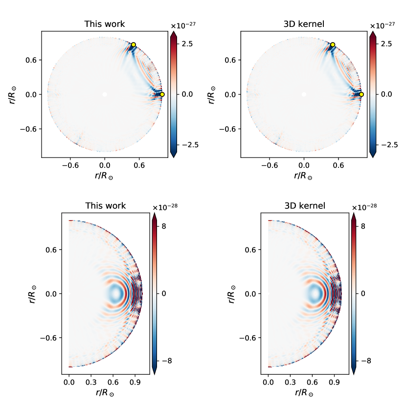
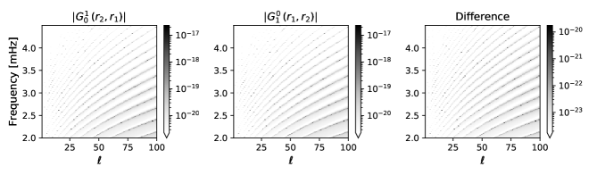
We plot an equatorial cross-section of the three-dimensional kernel evaluated at $r=R_{\odot}$ in the top left panel of Figure 6, choosing the two observation points $\mathbf{x}_{1}$ and $\mathbf{x}_{2}$ to be $\left(R_{\odot}+200\text{km},\frac{\pi}{2},0\right)$ and $\left(R_{\odot}+200\text{km},\frac{\pi}{2},\frac{\pi}{3}\right)$ respectively, and compare it with the same computed using Equation 43 in the top right panel. We impose the cutoff $j_{1},j_{2}<=80$ on the angular degrees of the waves keeping numerical accuracy in mind, which translates to a cutoff of $\ell<=160$ on the kernel components through the triangle inequality. We have multiplied the kernel by the sound-speed profile to highlight the radial profile. We find a good match between the two functions, which affirms the correctness of the analysis. The bottom left and bottom right panels of Figure 6 show meridional cross-sections of the same functions evaluated at $\phi=\pi/6$.

Figure 6: Equatorial slice (top) and meridional slice (bottom) of $cK_{c}\left(\mathbf{x},\mathbf{x}_{1},\mathbf{x}_{2}\right)$ for $\mathbf{x}_{1}=\left(R_{\odot}+200\text{km},\pi/2,0\right)$ and $\mathbf{x}_{2}=\left(R_{\odot}+200\text{km},\pi/2,\pi/3\right)$, computed in the radial line-of-sight assumption. The left panel in each case is computed by summing over the spherical harmonic components using Equation (42), whereas the right panel is computed by starting from the fleshed-out Green functions using Equation (43). The yellow dots denote the location of the two observation points. The meridional cross-section has been computed at $\phi=\pi/6$, which is halfway between the longitudes of the two observation points. The color scales have been saturated to highlight the deep-lying features.

5.3 Validating the travel-time kernel: isotropic perturbation

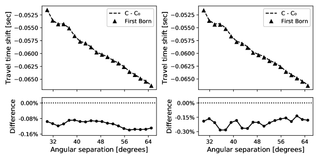
We verify the expression for the kernel by using an isotropic $\delta c\left(r\right)$ and computing wave travel-time shifts between the point $\mathbf{x}_{1}=\left(R_{\odot}+200\text{km},\frac{\pi}{2},0\right)$ and $\mathbf{x}_{2}=\left(R_{\odot}+200\text{km},\frac{\pi}{2},\phi\right)$ for various choices of $\phi$. The corresponding kernel may be obtained by substituting $\ell=m=0$ in Equation (41). We also compute the kernel for the radial components of the displacement, and compute the travel times with the resultant expression to compare with Mandal et al. (2017). The expression for the kernel using just the radial components simplifies to

$$K_{00}\left(r,\mathbf{x}_{1},\mathbf{x}_{2}\right) =\frac{1}{\sqrt{4\pi}}\int_{0}^{\infty}\frac{d\omega}{2\pi}\,\omega^{2}P\left(\omega\right)\sum_{j}\frac{\left(2j+1\right)}{4\pi}\,2\Re\left[h^{*}\left(\mathbf{x}_{\text{1}},\mathbf{x}_{2},\omega\right)T_{0,jj\omega}^{0}\left(r,r_{1},r_{2},r_{\text{src}}\right)\right]P_{j}\left(\hat{n}_{\text{1}}\cdot\hat{n}_{2}\right),$$ (46)

where $P_{j}$ represents the Legendre polynomial of degree $j$.

We also compute travel time shifts using Equation (39) for the same sets of points, where we compute the change in cross covariance $\delta C$ as an explicit difference between the cross covariance $C$ evaluated in the two background models. We plot both sets of travel times in Figure 7, with and without line-of-sight projection. We find that the measured travel times in both the cases are quite similar. This is a consequence of the result that the travel-time kernel components for $\ell=0$ and $m=0$ are nearly identical with and without projection.

Figure 7: Travel time shifts between two models having radial sound-speed profiles $c\left(r\right)\times\left(1+10^{-5}\right)$ and $c\left(r\right)$, using waves measured at the two points $\mathbf{x}_{1}=\left(R_{\odot}+200\text{km},\pi/2,0\right)$ and $\mathbf{x}_{2}=\left(R_{\odot}+200\text{km},\pi/2,\phi\right)$ for various different values of the angular separation $\phi$. The left panel is using radial components of the waves, whereas the right panel uses the line-of-sight projected components.

5.4 Computational efficiency

One of the advantages of this approach over evaluating the spherical harmonic coefficients of the three-dimensional kernel $K(\mathbf{x},\mathbf{x}_{2},\mathbf{x}_{2})$ is that the evaluations of the kernel components are much more efficient if we are interested in a limited number of them. To demonstrate this, we evaluate the kernels $K_{\ell m}(r)$ using our approach, and the coefficients

$$K^{3D}_{\ell m}(r)=\int d\Omega\,Y_{\ell m}^{*}(\hat{n})K(\mathbf{x}=(r,\hat{n}),\mathbf{x}_{2},\mathbf{x}_{2}),$$ (47)

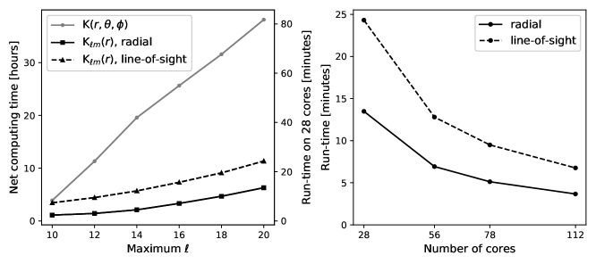
and compare the evaluation time in the two approaches. The latter involves two steps — evaluating the three-dimensional profile of the kernel $K(\mathbf{x},\mathbf{x}_{2},\mathbf{x}_{2})$, followed by a decomposition in the basis of spherical harmonics, where the second step is significantly faster than the first one. We therefore list the time taken only to evaluate the kernel $K(\mathbf{x},\mathbf{x}_{2},\mathbf{x}_{2})$. In the first case we compute the kernel components for all the modes $(\ell,m)$ for $-\ell\leq m\leq\ell$ and $\ell\leq\ell_{\mathrm{max}}$, whereas in the latter we compute the three-dimensional profile for co-latitude $\theta$ corresponding to $\left(\ell_{\mathrm{max}}+1\right)/2$ Gauss-Legendre nodes, and $2\ell_{\text{max}}$ uniformly spaced points in the azimuthal coordinate $\phi$ ranging from $0$ to $2\pi$. The computation is carried out by summing over Green functions having angular degrees in the range $5\leq j\leq 80$ and $4000$ uniformly spaced frequencies in the range $2\,\text{mHz}$ to $4.5\,\text{mHz}$. We arbitrarily choose the two observation points to be $\mathbf{x}_{1}=(R_{\odot}+200\,\text{km},\pi/6,-\pi/4)$ and $\mathbf{x}_{2}=(R_{\odot}+200\,\text{km},-\pi/3,\pi/4)$. We carry out the computation on one node of the Dalma cluster at New York University Abu Dhabi, that has $28$ processors available. We compare the evaluation times in Figure 8, where we show that the spherical-harmonic components in both the radial and line-of-sight-projected approaches may be computed significantly faster than the three-dimensional profile. The evaluation times shown in Figure 8 are not to be treated as absolute limits as further optimization is possible; however, they suffice to demonstrate the trend in the comparative analysis presented here. The evaluation times would also be lower for points having special geometrical locations — such as poles or being located on the Equator — in which case various spherical-harmonic symmetries might lead to cancellations in the terms being summed. Such an approach, along with rotating the kernels components on the sphere, might lead to rapid evaluation of kernel components.

The radial parts $T_{\alpha,j_{1}j_{2}\omega}^{\beta}\left(r,r_{1},r_{2},r_{\text{src}}\right)$ of the kernels $K_{\ell m}$ in Equation. 41 do not depend on $\ell$, which provides a major computational advantage as they need to be computed only once for each combination of $(j_{1},j_{2},\omega)$ and may be reused for each $(\ell,m)$. This result arises from the fact that the sound-speed perturbation acts as a multiplicative scalar term in Equation 24, and the result is not expected to hold for other parameters such as flow velocity. We therefore expect the computation of kernels for such parameters to be more resource intensive.

Figure 8: Left: Computational time required to evaluate the kernel components compared with that required to compute the three-dimensional kernel $K(r,\theta,\phi)$ following Mandal et al. (2017). The solid black line represents time taken to compute kernels using only the radial components of the wave displacement, whereas the dashed black line represents that for line-of-sight projected components of wave displacement. Right: Evaluation time as a function of the number of cores used compute the kernel components.

6 Conclusion

The inference of solar subsurface features using surface measurements relies on an accurate estimate of the sensitivity kernel that relates the model parameters to the measurements. The sensitivity kernel incorporates the physics of wave propagation as well as the systematics involved in the measurement procedure. In this work we have illustrated an approach that lets us compute travel-time sensitivity kernels in the Sun while incorporating the systematic effects introduced by spherical geometry in the measurements, such as line-of-sight projection in Dopplergram measurements and center-to-limb differences in line-formation heights. Conventional helioseismic inversions have adjusted for these systematics by correcting the measured travel-times (Zhao et al., 2012), but a better understanding of the underlying physics might be obtained by a first-principle approach such as the one presented in this work.

The analysis presented in this work leads to the spherical-harmonic components of the sensitivity kernels. Large-scale features in the Sun may be expressed in an angular spherical harmonic basis in terms of a limited number of low-degree components. The present analysis therefore provides us with two advantages — firstly the computation is numerically efficient if seek only a few low-degree modes, and secondly the inverse problem is better conditioned if we limit the number of parameters being solved for.

In this work we have computed sensitivity kernels for sound-speed perturbations which is a scalar (rank-$0$) field. The analysis is however general in scope, and can be extended to tensors of any rank by using the definition of the angular derivative of a vector spherical harmonic (see Varshalovich et al., 1988). Of particular interest is the analysis of large-scale subsurface flows in the Sun such as meridional flows. Recently Mandal et al. (2018) had carried out an analysis of subsurface flows on a similar line by numerically projecting the $3$-dimensional sensitivity kernel on to a sparse basis. Our analysis demonstrates how such a decomposition can be arrived at analytically, thereby increasing the computational efficiency of the procedure.

Appendix A Radial components of Green functions

We choose to rewrite the wave equation in terms of the displacement $\bm{\xi}$, the pressure perturbation $p^{\prime}$ and the density perturbation $\rho^{\prime}$ as

$$\mathcal{L}\bm{\xi}=-\rho\omega^{2}\bm{\xi}-2i\omega\gamma\bm{\xi}+\bm{\nabla}p^{\prime}+\rho^{\prime}g\mathbf{e}_{r}=\mathbf{S}.$$ (A1)

The form of the wave equation naturally suggests the use of the Hansen VSH basis. We expand the vector wave displacement and source as

$$\bm{\xi}\left(\mathbf{x}\right) =\sum_{\ell m\alpha}\xi_{\ell m}^{\left(\alpha\right)}\left(r\right)\mathbf{Y}_{\ell m}^{\left(\alpha\right)},$$ (A2)

$$\mathbf{S}\left(\mathbf{x}\right) =\sum_{\ell m\alpha}S_{\ell m}^{\left(\alpha\right)}\left(r\right)\mathbf{Y}_{\ell m}^{\left(\alpha\right)}.$$ (A3)

and the scalar pressure and density perturbations as

$$p^{\prime}\left(\mathbf{x}\right) =\sum_{\ell m}p_{\ell m}^{\prime}\left(r\right)Y_{\ell m}\left(\hat{n}\right),$$ (A4)

$$\rho^{\prime}\left(\mathbf{x}\right) =\sum_{\ell m}\rho_{\ell m}^{\prime}\left(r\right)Y_{\ell m}\left(\hat{n}\right).$$ (A5)

Substituting these into Equation (A1), we obtain the components of the wave equation in the Hansen VSH basis:

$$-\rho\omega^{2}\xi_{\ell m}^{\left(-1\right)}+\partial_{r}p_{\ell m}^{\prime}+\rho_{\ell m}^{\prime}g =S_{\ell m}^{\left(-1\right)},$$

$$-\rho\omega^{2}\xi_{\ell m}^{\left(1\right)}+\frac{\sqrt{\ell\left(\ell+1\right)}}{r}p_{\ell m}^{\prime} =S_{\ell m}^{\left(1\right)}.$$ (A6)

In addition to this, we use the continuity equation

$$\rho^{\prime}+\bm{\nabla}\cdot\left(\rho_{0}\bm{\xi}\right)=0,$$ (A7)

which is expanded in terms of the components of $\bm{\xi}$ as

$$\rho_{\ell m}^{\prime}=-\frac{1}{r^{2}}\partial_{r}\left(r^{2}\rho_{0}\xi_{\ell m}^{\left(-1\right)}\right)+\frac{\sqrt{\ell\left(\ell+1\right)}}{r}\rho_{0}\xi_{\ell m}^{\left(1\right)},$$ (A8)

and the adiabatic equation of state

$$\rho_{\ell m}^{\prime}=\frac{1}{c^{2}}p_{\ell m}^{\prime}+\frac{\rho_{0}N^{2}}{g_{0}}\xi_{\ell m}^{\left(-1\right)},$$ (A9)

where the Brunt-Väisälä frequency $N$ is defined in terms of the thermal structure parameters $\rho_{0}$, $p_{0}$, $g_{0}$ and the adiabatic index $\Gamma_{1}$ as

$$N^{2}=g_{0}\left(\frac{1}{\Gamma_{1}}\frac{d\ln p_{0}}{dr}-\frac{d\ln\rho_{0}}{dr}\right).$$

We use Equations (A8) and (A9) to eliminate the variables $\rho_{\ell m}^{\prime}$ and $\xi_{\ell m}^{\left(1\right)}$ from Equation (A6) and obtain equations in the variables $\xi_{\ell m}^{\left(-1\right)}$ and $p^{\prime}$. The reason we choose these two variables is that we enforce the Dirichlet boundary conditions $\xi_{\ell m}^{\left(-1\right)}\left(r=0\right)=0$ and $p^{\prime}\left(r=r_{\text{out}}\right)=0$, where $r_{\text{out}}$ is the outer boundary of the computational domain. The system of equations for $\xi_{\ell m}^{\left(-1\right)}$ and $p^{\prime}$ therefore becomes

$$\left(\begin{array}[]{cc}-\rho_{0}\left(\omega^{2}-N^{2}\right)&\partial_{r}+\frac{g_{0}}{c^{2}}\\ \partial_{r}+\frac{2}{r}-\frac{g_{0}}{c^{2}}&\frac{1}{\rho_{0}c^{2}}\left(1-\frac{S_{\ell}^{2}}{\omega^{2}}\right)\end{array}\right)\left(\begin{array}[]{c}\xi_{\ell m}^{\left(-1\right)}\\ p_{\ell m}^{\prime}\end{array}\right)=\left(\begin{array}[]{c}S_{\ell m}^{\left(-1\right)}\\ -\frac{\sqrt{\ell\left(\ell+1\right)}}{\omega^{2}}\frac{1}{r\rho_{0}}S_{\ell m}^{\left(1\right)}\left(r\right)\end{array}\right),$$ (A10)

and we compute the horizontal displacement $\xi_{\ell m}^{\left(1\right)}\left(r\right)$ through

$$\xi_{\ell m}^{\left(1\right)}\left(r\right)=\frac{\sqrt{\ell\left(\ell+1\right)}}{\rho_{0}r\omega^{2}}p_{\ell m}^{\prime}\left(r\right)-\frac{1}{\rho_{0}\omega^{2}}S_{\ell m}^{\left(1\right)}\left(r\right).$$ (A11)

The Green function for the operator $\mathcal{L}$ satisfies

$$\mathcal{L}\mathbf{G}\left(\mathbf{x},\mathbf{x}_{\text{src}};\omega\right)=\delta\left(\mathbf{x}-\mathbf{x}_{\text{src}}\right)\mathbf{I},$$ (A12)

where $\delta\left(\mathbf{x}-\mathbf{x}_{\text{src}}\right)$ is the Dirac delta function centered about the point $\mathbf{x}_{\text{src}}$, $\mathbf{I}$ is the $3\times 3$ identity matrix and $\omega$ represents temporal frequency. The wave operator $\mathcal{L}$ is spherically symmetric in the quiet Sun, and its eigenfunctions are labeled by radial order $n$ and angular degrees $j$ and $m$. The Green function is expanded in the Hansen VSH basis as

$$\mathbf{G}\left(\mathbf{x},\mathbf{x}_{\text{src}};\omega\right)=\sum_{\alpha,\beta=-1}^{1}\sum_{\ell m}G_{\left(\beta\right),\ell\omega}^{\left(\alpha\right)}\left(r,r_{\text{src}}\right)\mathbf{Y}_{\ell m}^{\left(\alpha\right)}\left(\hat{n}\right)\mathbf{Y}_{\ell m}^{\left(\beta\right)\dagger}\left(\hat{n}_{\text{src}}\right)$$ (A13)

Solving for the Green function is therefore equivalent to obtaining the radial components $G_{\left(\beta\right),\ell\omega}^{\left(\alpha\right)}\left(r,r_{\text{src}}\right)$. We note that spherical symmetry of the wave operator implies that the components of the Green function do not depend on the azimuthal quantum number $m$. We also note that the delta function source is expanded as

$$\delta\left(\mathbf{x}-\mathbf{x}_{\text{src}}\right)\mathbf{I}=\frac{1}{r^{2}}\delta\left(r-r_{\text{src}}\right)\sum_{\alpha=-1}^{1}\sum_{\ell m}\mathbf{Y}_{\ell m}^{\left(\alpha\right)}\left(\hat{n}\right)\mathbf{Y}_{\ell m}^{\left(\alpha\right)\dagger}\left(\hat{n}_{\text{src}}\right).$$

Substituting these into Equation (A10) we obtain

$$\left(\begin{array}[]{cc}-\rho_{0}\left(\omega^{2}-N^{2}\right)&\partial_{r}+\frac{g_{0}}{c^{2}}\\ \partial_{r}+\frac{2}{r}-\frac{g_{0}}{c^{2}}&\frac{1}{\rho_{0}c^{2}}\left(1-\frac{S_{\ell}^{2}}{\omega^{2}}\right)\end{array}\right)\left(\begin{array}[]{c}G_{\left(\beta\right),\ell\omega}^{\left(-1\right)}\left(r,r_{\text{src}}\right)\\ p_{\left(\beta\right),\ell\omega}^{\prime}\left(r,r_{\text{src}}\right)\end{array}\right)=\frac{1}{r^{2}}\delta\left(r-r_{\text{src}}\right)\left(\begin{array}[]{c}\delta_{\beta}^{-1}\\ -\frac{\sqrt{\ell\left(\ell+1\right)}}{\omega^{2}}\frac{1}{r\rho_{0}}\delta_{\beta}^{1}\end{array}\right),$$ (A14)

and subsequently using (A11) we obtain

$$G_{\left(\beta\right),\ell\omega}^{\left(1\right)}\left(r,r_{\text{src}}\right)=\frac{\sqrt{\ell\left(\ell+1\right)}}{\rho_{0}r\omega^{2}}\left(p_{\left(\beta\right),\ell\omega}^{\prime}\left(r,r_{\text{src}}\right)-\frac{1}{r^{2}}\delta\left(r-r_{\text{src}}\right)\delta_{\beta}^{1}\right).$$ (A15)

The components of the Green function obey certain symmetry conditions that arise from that fact that the eigenfunctions of the wave operator $\mathcal{L}$ are strictly spheroidal, and may be expanded in the Hansen VSH basis in terms of the vectors $\mathbf{Y}_{\ell m}^{\left(-1\right)}$ and $\mathbf{Y}_{\ell m}^{\left(1\right)}$ without any component along $\mathbf{Y}_{\ell m}^{\left(0\right)}$. This is seen from Equation (A6) by noting that the restoring force has no component along $\mathbf{Y}_{\ell m}^{\left(0\right)}$. This implies that the summations over $\alpha$ and $\beta$ in Equation (A13) only range over $\pm 1$. This leads to the following symmetry conditions in the PB VSH basis:

$$G_{+,\ell\omega}^{\alpha} =G_{-,\ell\omega}^{\alpha},\quad\alpha\in\left\{+,0,-\right\},$$ (A16)

$$G_{\alpha,\ell\omega}^{+} =G_{\alpha,\ell\omega}^{-},\quad\alpha\in\left\{+,0,-\right\}.$$

These symmetry relations imply that there are four independent components of the Green’s function. Without loss of generality, we choose the components

$$G_{0,\ell\omega}^{0} =G_{\left(-1\right),\ell\omega}^{\left(-1\right)},\quad G_{0,\ell\omega}^{+}=\frac{1}{\sqrt{2}}G_{\left(-1\right),\ell\omega}^{\left(1\right)},$$ (A17)

$$G_{+,\ell\omega}^{0} =\frac{1}{\sqrt{2}}G_{\left(1\right),\ell\omega}^{\left(-1\right)},\quad G_{+,\ell\omega}^{+}=\frac{1}{2}G_{\left(1\right),\ell\omega}^{\left(1\right)}.$$

These represent the radial and tangential responses to a radial and tangential source respectively, where the tangential direction is specifically oriented along $\mathbf{Y}_{\ell m}^{+}$ at each point on the Sun. We solve Equations (A10) and (A11) for the Hansen VSH components $G_{\left(\pm 1\right),\ell\omega}^{\left(\pm 1\right)}$ of the Green function, and use these to compute the PB VSH components $G_{\pm 1,\ell\omega}^{\pm 1}$ using Equation (A17).

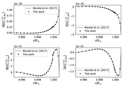
Equation (A10) is equivalent to that obtained by Mandal et al. (2017), where the authors had solved for just the components $G_{\left(-1\right),\ell\omega}^{\left(-1\right)}$ and $G_{\left(-1\right),\ell\omega}^{\left(+1\right)}$ corresponding to radial and tangential displacements for a radially directed source respectively. The other components appear in the expression for the kernel if we consider line-of-sight projection effects, so we choose to solve for all of them. We solve Equation (A10) numerically using a high-order finite-difference solver similar to the one described by Mandal et al. (2017) using sparse-matrix representation of the operators implemented in the Julia language (Bezanson et al., 2017). We use Model S (Christensen-Dalsgaard et al., 1996) as our background solar model to compute the Green functions. We compare our Green functions to those obtained by Mandal et al. (2017) in Figure 9.

Figure 9: The Green functions computed in this work compared to those computed earlier by Mandal et al. (2017). The top row shows the real and imaginary parts of the radial component of the Green function for a radial source, whereas the bottom row shows the tangential component of the Green function for a radial source. The Green function has been computed for $\ell=40$ and $\nu=3\,\text{mHz}$.

We note that Equation (A14) implies certain discontinuities in the Green function components at the source radius. Assuming a radial delta-function source we integrate the equations over $\left[r_{\text{src}}-\varepsilon,\,r_{\text{src}}+\varepsilon\right]$ where $\varepsilon\rightarrow 0$ to obtain

$$p_{\left(-1\right),\ell\omega}^{\prime}\left(r_{\text{src}}+\varepsilon,r_{\text{src}}\right)-p_{\left(-1\right),\ell\omega}^{\prime}\left(r_{\text{src}}-\varepsilon,r_{\text{src}}\right)=\frac{1}{r_{\text{src}}^{2}}.$$

On the other hand assuming a tangential delta function source we obtain

$$G_{\left(1\right),\ell\omega}^{\left(-1\right)}\left(r_{\text{src}}+\varepsilon,r_{\text{src}}\right)-G_{\left(1\right),\ell\omega}^{\left(-1\right)}\left(r_{\text{src}}-\varepsilon,r_{\text{src}}\right)=-\frac{\sqrt{\ell\left(\ell+1\right)}}{\omega^{2}}\frac{1}{r_{\text{src}}^{3}\rho_{0}\left(r_{\text{src}}\right)}.$$

The discontinuity in $G_{\left(1\right),\ell\omega}^{\left(-1\right)}$ at $r_{\text{src}}$ implies a singularity in $G_{\left(1\right),\ell\omega}^{\left(1\right)}$ which is related to its derivative. We also see this from Equation (A15).

A.1 Seismic reciprocity

The wave operator $\mathcal{L}$ has an adjoint $\mathcal{L}^{\dagger}$ defined as

$$\int d\mathbf{x}\,\mathbf{u}_{k}^{*}\left(\mathbf{x}\right)\cdot\mathcal{L}\mathbf{v}_{m}\left(\mathbf{x}\right)=\int d\mathbf{x}\,\left(\mathcal{L}^{\dagger}\mathbf{u}_{k}\left(\mathbf{x}\right)\right)^{*}\cdot\mathbf{v}_{m}\left(\mathbf{x}\right)$$ (A18)

for any pair of functions $\mathbf{u}_{k}\left(\mathbf{x}\right)$ and $\mathbf{v}_{m}\left(\mathbf{x}\right)$. The Green function $\mathbf{G}\left(\mathbf{x},\bm{\xi}\right)$ and the adjoint Green function $\mathbf{G}^{\dagger}\left(\mathbf{x},\bm{\xi}\right)$ satisfy

$$\mathcal{L}\mathbf{G}\left(\mathbf{x},\bm{\xi}\right)=\mathcal{L}^{\dagger}\mathbf{G}^{\dagger}\left(\mathbf{x},\bm{\xi}\right)=\delta\left(\mathbf{x}-\bm{\xi}\right)\mathbf{I}.$$

We choose $\mathbf{u}_{k}\left(\mathbf{x}\right)$ and $\mathbf{v}_{m}\left(\mathbf{x}\right)$ in Equation (A18) to be spherical polar components of the Green functions given by

$$\mathbf{u}_{k}\left(\mathbf{x}\right) =\mathbf{G}^{\dagger}\left(\mathbf{x},\bm{\xi}^{\prime},\omega\right)\cdot\mathbf{e}_{k}\left(\bm{\xi}^{\prime}\right),$$

$$\mathbf{v}_{m}\left(\mathbf{x}\right) =\mathbf{G}\left(\mathbf{x},\bm{\xi},\omega\right)\cdot\mathbf{e}_{m}\left(\bm{\xi}\right),$$

to obtain the relation $G_{mk}^{\dagger}\left(\bm{\xi},\bm{\xi}^{\prime}\right)=G_{km}^{*}\left(\bm{\xi}^{\prime},\bm{\xi}\right)$, or in a compact notation $\mathbf{G^{\dagger}}\left(\bm{\xi},\bm{\xi}^{\prime}\right)=\left[\mathbf{G}\left(\bm{\xi}^{\prime},\bm{\xi}\right)\right]^{\dagger}.$ We further use the fact that $\mathcal{L}^{\dagger}=\mathcal{L}^{*}$ and hence $\mathbf{G}^{\dagger}\left(\bm{\xi},\bm{\xi}^{\prime}\right)=\mathbf{G}^{*}\left(\bm{\xi},\bm{\xi}^{\prime}\right)$ to obtain the reciprocity relation $\mathbf{G}\left(\bm{\xi}^{\prime},\bm{\xi}\right)=\mathbf{G}^{T}\left(\bm{\xi},\bm{\xi}^{\prime}\right).$ Expanding the Green tensor in the PB VSH basis we show that the components are related by $G_{\beta,\ell\omega}^{\alpha}\left(r,r^{\prime}\right)=G_{-\alpha,\ell\omega}^{-\beta}\left(r^{\prime},r\right)$. In addition to this, if we enforce the condition that the Green function is strictly spheroidal we may use the symmetries in Equation (A16) to rewrite this as

$$G_{\beta,\ell\omega}^{\alpha}\left(r,r^{\prime}\right)=G_{\alpha,\ell\omega}^{\beta}\left(r^{\prime},r\right).$$ (A19)

We obtain similar relations in the Hansen basis with the superscript and subscript indices interchanged in each case. We plot $\left|G_{0,\ell\omega}^{1}\left(r_{2},r_{1}\right)\right|$ and $\left|G_{1,\ell\omega}^{0}\left(r_{1},r_{2}\right)\right|$ in Figure 10, choosing the values $r_{1}=R_{\odot}-75\,\text{km}$ and $r_{2}=R_{\odot}+200\,\text{km}$. We find a reasonably good match, verifying the validity of the reciprocity relation.

Figure 10: Absolute values of Green function components. Left: tangential component of displacement for a radial source, middle panel: radial component of displacement for a tangential source, right: difference between the components.

Appendix B Three-dimensional kernel

A change in cross-covariance of the radial components of displacement may be expressed as

$$\delta C_{rr}\left(\mathbf{x}_{1},\mathbf{x}_{2};\omega\right) =\omega^{2}P\left(\omega\right)\int d\Omega_{\text{src}}\,\left[\delta G_{rr}^{*}\left(\mathbf{x}_{1},\mathbf{x}_{\text{src}};\omega\right)G_{rr}\left(\mathbf{x}_{2},\mathbf{x}_{\text{src}};\omega\right)+G_{rr}^{*}\left(\mathbf{x}_{1},\mathbf{x}_{\text{src}};\omega\right)\delta G_{rr}\left(\mathbf{x}_{2},\mathbf{x}_{\text{src}};\omega\right)\right],$$ (B1)

where the radial component of the Green function is obtained from Equation (17) to be

$$G_{rr}\left(\mathbf{x}_{i},\mathbf{x}_{\text{src}};\omega\right)=\sum_{j}\frac{\left(2j+1\right)}{4\pi}G_{rrj\omega}\left(r_{i},r_{\text{src}}\right)P_{j}\left(\hat{n}_{i}\cdot\hat{n}_{\text{src}}\right),$$

and the change in the radial component due to a local sound-speed inhomogeneity $\delta c\left(\mathbf{x}\right)$ may be represented as

$$\delta G_{rr}\left(\mathbf{x}_{\text{obs}},\mathbf{x}_{\text{src}},\omega\right)=-2\int d\mathbf{x}\,\rho c\bm{\nabla}\cdot\mathbf{G}_{r}\left(\mathbf{x},\mathbf{x}_{\text{obs}},\omega\right)\bm{\nabla}\cdot\mathbf{G}_{r}\left(\mathbf{x},\mathbf{x}_{\text{src}},\omega\right)\delta c\left(\mathbf{x}\right).$$

The radial component of the divergence may be calculated to be

$$\bm{\nabla}\cdot\mathbf{G}_{r}\left(\mathbf{x},\mathbf{x}_{i};\omega\right)=\sum_{j}\frac{\left(2j+1\right)}{4\pi}\left[\bm{\nabla}\cdot\mathbf{G}\right]_{rj\omega}\left(r,r_{i}\right)P_{j}\left(\hat{n}\cdot\hat{n}_{i}\right),$$

where the radial profile $\left[\bm{\nabla}\cdot\mathbf{G}\right]_{rj\omega}\left(r,r_{i}\right)$ is given by the $\beta=0$ term in Equation (18). The kernel is defined through the equation

$$d\tau\left(\mathbf{x}_{1},\mathbf{x}_{2}\right)=\int d\mathbf{x}\,K\left(\mathbf{x},\mathbf{x}_{1},\mathbf{x}_{2}\right)\delta c\left(\mathbf{x}\right).$$ (B2)

Substituting Equation (B1) into Equation (39) and recasting it into the form of Equation (B2), we obtain

$$K\left(\mathbf{x},\mathbf{x}_{1},\mathbf{x}_{2}\right) =\int_{0}^{\infty}\frac{d\omega}{2\pi}\,\omega^{2}P\left(\omega\right)\sum_{j_{1}j_{2}}\frac{\left(2j_{1}+1\right)}{4\pi}\frac{\left(2j_{2}+1\right)}{4\pi}P_{j_{1}}\left(\hat{n}\cdot\hat{n}_{1}\right)P_{j_{2}}\left(\hat{n}\cdot\hat{n}_{2}\right)\times$$

$$2\Re\left[h^{*}\left(\mathbf{x}_{1},\mathbf{x}_{2},\omega\right)T_{0,j_{1}j_{2}\omega}^{0}\left(r,r_{1},r_{2},r_{\text{src}}\right)\right].$$

We simplify the angular function

$$A=\frac{\left(2j_{1}+1\right)}{4\pi}\frac{\left(2j_{2}+1\right)}{4\pi}P_{j_{1}}\left(\hat{n}\cdot\hat{n}_{1}\right)P_{j_{2}}\left(\hat{n}\cdot\hat{n}_{2}\right)$$

by using rewriting the expression in terms of spherical harmonics. We use the expansion of Legendre polynomials in terms of spherical harmonics:

$$\frac{\left(2j+1\right)}{4\pi}P_{j}\left(\hat{n}\cdot\hat{n}_{i}\right)=\sum_{m=-j}^{j}Y_{jm}\left(\hat{n}\right)Y_{jm}^{*}\left(\hat{n}_{i}\right)$$

to obtain the angular term to be

$$A=\sum_{m_{1}=-j_{1}}^{j_{1}}\sum_{m_{2}=-j_{2}}^{j_{2}}Y_{j_{1}m_{1}}\left(\hat{n}\right)Y_{j_{2}m_{2}}\left(\hat{n}\right)Y_{j_{1}m_{1}}^{*}\left(\hat{n}_{1}\right)Y_{j_{2}m_{2}}^{*}\left(\hat{n}_{2}\right).$$

We use the angular momentum coupling relation

$$Y_{j_{1}m_{1}}\left(\hat{n}\right)Y_{j_{2}m_{2}}\left(\hat{n}\right)=\sum_{jm}\sqrt{\frac{\left(2j_{1}+1\right)\left(2j_{2}+1\right)}{4\pi\left(2j+1\right)}}C_{j_{1}0j_{2}0}^{j0}C_{j_{1}m_{1}j_{2}m_{2}}^{jm}Y_{jm}\left(\hat{n}\right)$$

(see Varshalovich et al., 1988) to obtain

$$A=\sum_{jm}\sqrt{\frac{\left(2j_{1}+1\right)\left(2j_{2}+1\right)}{4\pi\left(2j+1\right)}}C_{j_{1}0j_{2}0}^{j0}Y_{jm}^{j_{1}j_{2}*}\left(\hat{n}_{1},\hat{n}_{2}\right)Y_{jm}\left(\hat{n}\right).$$

We identify the constant pre-factor to be $N_{j_{1}j_{2}j}$ from Equation (35).

References

- Bezanson et al. (2017) Bezanson, J., Edelman, A., Karpinski, S., & Shah, V. 2017, SIAM Review, 59, 65, doi: 10.1137/141000671
- Birch & Gizon (2007) Birch, A. C., & Gizon, L. 2007, Astronomische Nachrichten, 328, 228, doi: 10.1002/asna.200610724
- Birch & Kosovichev (2000) Birch, A. C., & Kosovichev, A. G. 2000, Sol. Phys., 192, 193, doi: 10.1023/A:1005283526062
- Birch et al. (2001) Birch, A. C., Kosovichev, A. G., Price, G. H., & Schlottmann, R. B. 2001, ApJ, 561, L229, doi: 10.1086/324766
- Böning et al. (2016) Böning, V. G. A., Roth, M., Zima, W., Birch, A. C., & Gizon, L. 2016, ApJ, 824, 49, doi: 10.3847/0004-637X/824/1/49
- Chandrasekhar & Kendall (1957) Chandrasekhar, S., & Kendall, P. C. 1957, ApJ, 126, 457, doi: 10.1086/146413
- Christensen-Dalsgaard (1997) Christensen-Dalsgaard, J. 1997, Lecture Notes on Stellar Oscillations. https://citeseerx.ist.psu.edu/viewdoc/summary?doi=10.1.1.47.9910
- Christensen-Dalsgaard et al. (1996) Christensen-Dalsgaard, J., Dappen, W., Ajukov, S. V., et al. 1996, Science, 272, 1286, doi: 10.1126/science.272.5266.1286
- Dahlen & Tromp (1998) Dahlen, F. A., & Tromp, J. 1998, Theoretical Global Seismology (Princeton University Press)
- Duvall et al. (1993) Duvall, T. L., J., Jefferies, S. M., Harvey, J. W., & Pomerantz, M. A. 1993, Nature, 362, 430, doi: 10.1038/362430a0
- Feng et al. (2015) Feng, X. M., Wang, P., Yang, W., & Jin, G. R. 2015, Phys. Rev. E, 92, 043307, doi: 10.1103/PhysRevE.92.043307
- Fleck et al. (2011) Fleck, B., Couvidat, S., & Straus, T. 2011, Sol. Phys., 271, 27, doi: 10.1007/s11207-011-9783-9
- Fournier et al. (2018) Fournier, D., Hanson, C. S., Gizon, L., & Barucq, H. 2018, A&A, 616, A156, doi: 10.1051/0004-6361/201833206
- Gizon & Birch (2002) Gizon, L., & Birch, A. C. 2002, ApJ, 571, 966, doi: 10.1086/340015
- Gizon et al. (2017) Gizon, L., Barucq, H., Duruflé, M., et al. 2017, A&A, 600, A35, doi: 10.1051/0004-6361/201629470
- Hanasoge (2017) Hanasoge, S. M. 2017, MNRAS, 470, 2780, doi: 10.1093/mnras/stx1342
- Hanasoge & Duvall (2007) Hanasoge, S. M., & Duvall, T. L., J. 2007, Astronomische Nachrichten, 328, 319, doi: 10.1002/asna.200610737
- Hansen (1935) Hansen, W. W. 1935, Phys. Rev., 47, 139, doi: 10.1103/PhysRev.47.139
- James (1976) James, R. W. 1976, Philosophical Transactions of the Royal Society of London Series A, 281, 195, doi: 10.1098/rsta.1976.0025
- Kitiashvili et al. (2015) Kitiashvili, I. N., Couvidat, S., & Lagg, A. 2015, ApJ, 808, 59, doi: 10.1088/0004-637X/808/1/59
- Kosovichev (1996) Kosovichev, A. G. 1996, ApJ, 461, L55, doi: 10.1086/309989
- Kosovichev & Duvall (1997) Kosovichev, A. G., & Duvall, T. L. 1997, in SCORe ’96: Solar Convection and Oscillations and their Relationship, ed. F. P. Pijpers, J. Christensen-Dalsgaard, & C. S. Rosenthal (Dordrecht: Springer Netherlands), 241–260. https://doi.org/10.1007/978-94-011-5167-2_26
- Kumar et al. (1990) Kumar, P., Duvall, T. L., Harvey, J. W., et al. 1990, in Progress of Seismology of the Sun and Stars, ed. Y. Osaki & H. Shibahashi (Berlin, Heidelberg: Springer Berlin Heidelberg), 87–92
- Limpanuparb & Milthorpe (2014) Limpanuparb, T., & Milthorpe, J. 2014, arXiv e-prints, arXiv:1410.1748. https://arxiv.org/abs/1410.1748
- Mandal et al. (2017) Mandal, K., Bhattacharya, J., Halder, S., & Hanasoge, S. M. 2017, ApJ, 842, 89, doi: 10.3847/1538-4357/aa72a0
- Mandal et al. (2018) Mandal, K., Hanasoge, S. M., Rajaguru, S. P., & Antia, H. M. 2018, ApJ, 863, 39, doi: 10.3847/1538-4357/aacea2
- Nagashima et al. (2017) Nagashima, K., Fournier, D., Birch, A. C., & Gizon, L. 2017, A&A, 599, A111, doi: 10.1051/0004-6361/201629846
- Nordlund & Stein (1991) Nordlund, Å., & Stein, R. F. 1991, Granulation: Non-adiabatic patterns and shocks (Berlin, Heidelberg: Springer Berlin Heidelberg), 141–146
- Phinney & Burridge (1973) Phinney, R. A., & Burridge, R. 1973, Geophysical Journal, 34, 451, doi: 10.1111/j.1365-246X.1973.tb02407.x
- Ritzwoller & Lavely (1991) Ritzwoller, M. H., & Lavely, E. M. 1991, ApJ, 369, 557, doi: 10.1086/169785
- Schou (1999) Schou, J. 1999, ApJ, 523, L181, doi: 10.1086/312279
- Stein & Nordlund (1989) Stein, R. F., & Nordlund, A. 1989, ApJ, 342, L95, doi: 10.1086/185493
- Varshalovich et al. (1988) Varshalovich, D. A., Moskalev, A. N., & Khersonskii, V. K. 1988, Quantum Theory of Angular Momentum (World Scientific Publishing Co), doi: 10.1142/0270
- Wachter (2008) Wachter, R. 2008, Solar Physics, 251, 491, doi: 10.1007/s11207-008-9197-5
- Wieczorek & Meschede (2018) Wieczorek, M. A., & Meschede, M. 2018, Geochemistry, Geophysics, Geosystems, 19, 2574, doi: 10.1029/2018GC007529
- Zhao & Kosovichev (2004) Zhao, J., & Kosovichev, A. G. 2004, ApJ, 603, 776, doi: 10.1086/381489
- Zhao et al. (2012) Zhao, J., Nagashima, K., Bogart, R. S., Kosovichev, A. G., & Duvall, T. L., J. 2012, ApJ, 749, L5, doi: 10.1088/2041-8205/749/1/L5