An autonomous out of equilibrium Maxwell’s demon for controlling the energy fluxes produced by thermal fluctuations

Abstract

An autonomous out of equilibrium Maxwell’s demon is used to reverse the natural direction of the heat flux between two electric circuits kept at different temperatures and coupled by the electric thermal noise. The demon does not process any information, but it achieves its goal by using a frequency dependent coupling with the two reservoirs of the system. There is no energy flux between the demon and the system, but the total entropy production (system+demon) is positive. The demon can be power supplied by thermocouples. The system and the demon are ruled by equations similar to those of two coupled Brownian particles and of the Brownian gyrator. Thus our results pave the way to the application of autonomous out equilibrium Maxwell demons to coupled nanosystems at different temperatures.

Nowadays the notion of Maxwell’s demon (MD) is generically used to indicate mechanisms that allow a system to execute tasks in apparent violation of the second law of thermodynamics, such as for example to produce work from a single heat bath and to transfer heat from cold to hot sources. To obtain this result the demon does not exchange energy with the system but it has a positive entropy production rate, which compensate the negative entropy production of the system. In general the increase in entropy is induced by the fact that the demon needs to analyze the information that it gathers on the system statusLutz and Ciliberto (2015); Parrondo et al. (2015). In experiments this apparent violation of the second law is obtained by feedback mechanisms which often require the use of external devices such as A/D converters, computers etc.Toyabe et al. (2010); Elouard et al. (2017); Admon et al. (2018); Masuyama et al. (2018). Several smart experiments Price et al. (2008); Koski et al. (2014, 2015) have implemented these feedback locally constructing in this way autonomous Maxwell demons, which do not need the use of external devices as the measure and the feedback are performed in the same place. Several autonomous Maxwell demons have been theoretically developedBarato and Seifert (2013); Shiraishi et al. (2015); Boyd et al. (2016); Rosinberg and Horowitz (2016); Lu and Jarzynski (2019), but they can be of difficult practical implementation in several devices such as colloidal particles and mesoscopic electric circuits at room temperature. However it has been recently introduced in ref.Sanchez et al. (2019) a new paradigm of MD based on an out of equilibrium device, which does not elaborate any information about the system status. It has been shown that the parameters of this device can be suitably tuned in such a way that it does not exchange energy (heat or work) with the system but it has a positive entropy production rate. Thus it has the two main requirements of an autonomous MD and it can be more easily experimentally realized because, in contrast to the commonly used definition of MD, it works without acquiring and analyzing any information about the system status.

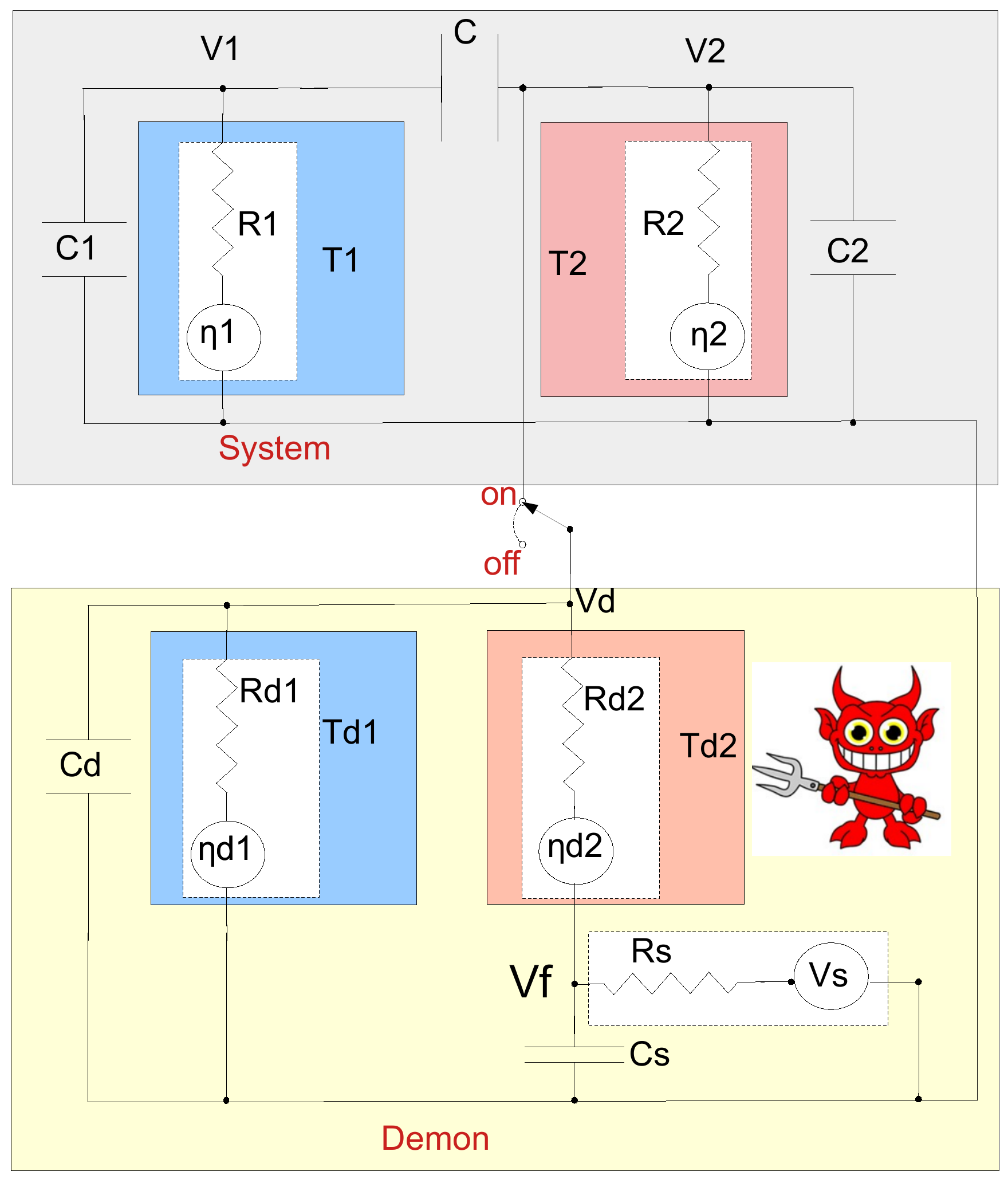
Figure 1: Diagram of the system (grey box) and of the demon (yellow box). The system is constituted by the two resistances $R_{1}$ and $R_{2}$ kept respectively at temperature $T_{1}$ and $T_{2}$, with $T_{2}\geq T_{1}$. They are coupled via the capacitor $C$. The capacitors $C_{1}$ and $C_{2}$ schematize the capacitances of the cables and of the amplifier inputs. The demon (yellow box), is composed by two resistances ($R_{d1}$ and $R_{d2}$) kept at two different temperatures $T_{d1}$ and $T_{d2}$.Furthermore the resistance $R_{d2}$ is driven by a voltage generator $V_{s}$ whose out-put is filtered by the low pas filter composed by the resistance $Rs$ and the capacitance $C_{s}$. The four voltage generators $\eta_{k}$ (k=1,2,d1,d2) represent the Nyquist noise voltages of the resistances at the temperatures of the heat baths.

We discuss here how to implement an out of equilibrium MD (OEMD) Sanchez et al. (2019) in electric circuits, which are versatile dynamical systems ruled by coupled Langevin equations Freitas et al. (2020); van Zon et al. (2004). Thus our study is quite general because it opens the way to the application of OEMDs to coupled nanosystems modeled by Langevin equations. As an example we will show in this article how an OEMD can be used to reverse the natural direction of the heat flux between two electric circuits kept at different temperatures and coupled by the electric thermal noise Ciliberto et al. (2013a, b). In fig.1 we sketch the system (gray box) and the demon (yellow box). We chose for the system this specific circuit because the statistical properties of the heat flux have been characterized both theoretically and experimentally Ciliberto et al. (2013a, b). Furthermore it is ruled by the same equations of the Brownian gyrator Filliger and Reimann (2007); Cerasoli et al. (2018) and of two Brownian particles coupled by a harmonic potential and kept at different temperaturesCiliberto et al. (2013a), making the result rather general

The system (grey box in fig.1) is constituted by two resistances $R_{1}$ and $R_{2}$, which are kept at two different temperatures $T_{1}$ and $T_{2}\geq T_{1}$. In the figure, the two resistances have been drawn with their associated thermal noise generators $\eta_{1}$ and $\eta_{2}$, whose power spectral densities are given by the Nyquist formula $|\tilde{\eta}_{m}|^{2}=4k_{B}R_{m}T_{m}$, with $m=1,2$. The coupling capacitance $C$ controls the electrical power exchanged between the resistances and as a consequence the energy exchanged between the two baths. No other coupling exists between the two resistances.. The two capacitors $C_{1}$ and $C_{2}$ represents the sum of the circuit and cable capacitances. All the relevant energy exchanges in the system can be derived by the simultaneous measurements of the voltage $V_{m}$ ($m=1,2$) across the resistance $R_{m}$ and the currents $i_{m}$ flowing through them. When $T_{1}=T_{2}$ the system is in equilibrium and exhibits no net energy flux between the two reservoirs. The circuit equations can be written in terms of charges $q_{m}$ flowed through the resistances $R_{m}$, so the measured instantaneous currents are $i_{m}=\dot{q}_{m}$. We make the choice of working with charges because the analogy with a Brownian particle is straightforward as $q_{m}$ is equivalent to the displacement of the particle $m$ van Zon et al. (2004); Ciliberto et al. (2013a, b). A circuit analysis shows that the equations for the charges are:

$$R_{1}\ \dot{q}_{1} = V_{1}-\eta_{1},\ \ \rm{and}\ \ \ R_{2}\ \dot{q}_{2}=\eta_{2}-V_{2},$$ (1)

with

$$V_{1} = \frac{-q_{1}(C+C_{2})+q_{2}\ C}{X}$$ (2)

$$V_{2} = \frac{-q_{1}\ C+q_{2}\ (C+C_{1})}{X}.$$ (3)

where $X=C_{2}\,C_{1}+C\,(C_{1}\,+C_{2})$ and $\eta_{m}$ is the Nyquist white noise: $\left<{\eta_{i}(t)\eta_{j}(t^{\prime})}\right>=2\delta_{ij}{k_{B}T_{i}R_{j}}\delta(t-t^{\prime})$. In ref.Ciliberto et al. (2013b) we have shown that eqs.1 fully characterize all the thermodynamics properties of the system.

In this system the work and the heat are defined as

$$\dot{W}_{m} = {C\over X}q_{m^{\prime}}\dot{q}_{m}$$ (4)

$$\dot{Q}_{m} = V_{m}i_{m}={V_{m}}\frac{V_{m}-\eta_{m}}{R_{m}}.$$ (5)

The quantities $\dot{W}_{m}$ is identified as the thermodynamic work performed by the circuit $m^{\prime}$ on $m\neq m^{\prime}$ and $Q_{m}$ the heat dissipated by the resistance $m$ van Zon et al. (2004); Freitas et al. (2020); Ciliberto et al. (2013a, b); Garnier and Ciliberto (2005). As all the variables are fluctuating, the derived quantities $\dot{Q}_{m}$ and $\dot{W}_{m}$ fluctuate too. In ref.Ciliberto et al. (2013a) we computed and measured the mean heat flux between the two heat baths, which is given by :

$$\left<{\dot{Q}_{1}}\right>=\ -\left<{\dot{Q}_{2}}\right>\ =\frac{C^{2}k_{B}(T_{2}-T_{1})}{XY}.$$ (6)

where $\left<{.}\right>$ stands for mean value and we have introduced the quantity $Y=\left[{(C_{1}+C)R_{1}+(C_{2}+C)R_{2}}\right]$. We use the convention that the heat extracted from a system reservoir is negative and the heat dissipated is positive.

The out of equilibrium demon is sketched in the yellow box of fig.1 and it is composed by two resistances ($R_{d1}$ and $R_{d2}$) kept at two different temperatures $T_{d1}$ and $T_{d2}$ (see Appendix A). The two voltage voltage generator $\eta_{d1}$ and $\eta_{d2}$ represent the Nyquist noise voltages associated to the two resistances at the heat bath temperatures. Furthermore the resistance $R_{d2}$ is driven by a voltage generator $V_{s}$ whose out-put is fltered by the the low pas filter composed by the resistance $Rs$ and the capacitance $C_{s}$(see Appendix A.1). We notice that demon scheme is similar to that of the system, with a coupling capacitance $C\rightarrow\infty$, on which the driving $V_{s}$ has been added. To design it, we followed the main prescriptions of ref.Sanchez et al. (2019): 1) It is out of equilibrium; 2) Either $T_{d1}$ or $T_{d2}$ has to be smaller than $T_{1}$; 3) it produces colored noise, obtained in our case by the source $V_{s}$ filtered by $R_{s}$ and $C_{s}$ ;4) It is coupled with the two parts of the system on different frequency ranges, specifically high frequencies with subsystem 1 and DC coupled with subsystem 2.

The choice of $V_{s}$ is very important in order to simplify the experimental configuration. Indeed $V_{s}$ can be either the thermal fluctuations of $Rs$ with a suitable cut-off imposed by the $R_{s}C_{s}$ or an external driving. Many choices are possible and the simplest one is to use $V_{s}=V_{f}$=constant and $Rs=0$. In such a way $V_{f}$ is coupled with $R_{2}$ only and the thermal noises $\eta_{d1}$ and $\eta_{d2}$ are directly coupled with $R_{2}$ and high pas filtered for $R_{1}$ (see Appendix A.1) The demon is always out of equilibrium, because, when it is disconnected from the system, the power supplied by $V_{f}$ is entirely dissipated in the demon resistances producing a mean heat flux towards the demon heat baths, even in the case $T_{d1}=T_{d2}$. This is a simplified version of the original OEMD of ref.Sanchez et al. (2019) because it requires the use of only one cold source at $T_{d}$ and a DC signal that can be easily generated by thermocouples making the demon fully autonomous. We will demonstrate that this demon can reverse the heat flux of the system in a wide range of parameters with a zero energy flux (heat and work) with the system.

The connection of the demon to the system changes the current distributions and the energy exchanges. The circuit analysis shows (see Appendix B), that the currents $\dot{q}_{k}$ ($k=1,2,d1,d2$) flowing in the resistances $R_{k}$ are now ruled by the following equations :

$$R_{1}\ \dot{q}_{1} = V_{1}-\eta_{1}$$ (7)

$$R_{2}\ \dot{q}_{2} = \eta_{2}-V_{2}$$ (8)

$$R_{d1}\ \dot{q}_{d1} = \eta_{d1}-V_{2}$$ (9)

$$R_{d2}\ \dot{q}_{d2} = \eta_{d2}+V_{f}-V_{2}$$ (10)

$$\ V_{1} = {-(C_{t}+C)\ q_{1}+\ C\ q_{t}\over X_{t}}$$ (11)

$$V_{2} = {(C_{1}+C)\ q_{t}-\ C\ q_{1}\over X_{t}}$$ (12)

where $q_{t}=(q_{2}+q_{d2}+q_{d1})$,$C_{t}=C_{2}+C_{d}$. and $X_{t}=C_{1}C_{t}+C(C_{1}+C_{t})$.

In order to reduce the number of parameters we consider the case $T_{d}=T_{d1}=T_{d2}$ and $R_{d1}=R_{d2}$. The heat fluxes in the four reservoirs can be computed using $\dot{Q}_{k}=v_{k}\dot{q}_{k}$, where $v_{k}$ is the potential difference on the resistance $R_{k}$ (see Appendix C). Introducing the following parameters $R_{d}=R_{d1}R_{d2}/(R_{d1}+R_{d2})$, $R_{t}=R_{d}R_{2}/(R_{d}+R_{2})$,
$Y_{t}=R_{1}\ (C+C_{1})+R_{t}\ (C+C_{t})$, $A={C^{2}k_{B}}/({X_{t}Y_{t}})$,
$\left<{V_{2}}\right>=V_{t}={V_{f}\ R_{t}/R_{d2}}$,
$B=A\ R_{t}\ (X_{t}R_{t}+R_{1}(C_{1}+C)^{2})/(R_{d}\ R_{2}\ C^{2})$,
we obtain:

$$\left<{\dot{Q}_{1}}\right> = A\left(\frac{R_{t}}{R_{2}}(T_{2}-T_{1})+\frac{R_{t}}{R_{d}}(T_{d}-T_{1})\right)$$ (13)

$$\left<{\dot{Q}_{2}}\right> = -A\frac{R_{t}}{R_{2}}(T_{2}-T_{1})-B(T_{2}-T_{d})\ +{V_{t}^{2}\over R_{2}}$$ (14)

$$\left<{\dot{Q}_{d}}\right> = -A\frac{R_{t}}{R_{d}}(T_{d}-T_{1})-B(T_{d}-T_{2})+$$ (15)

$$+\ {V_{f}^{2}R_{t}\over R_{d2}}({1\over R_{d1}}+{1\over R_{2}})-{V_{t}^{2}\over R_{2}}$$

$$\left<{\dot{W}_{f}}\right> = {V_{f}^{2}\ R_{t}\over R_{d2}}({1\over R_{d1}}+{1\over R_{2}})$$ (16)

where $\left<{\dot{Q}_{d}}\right>=\left<{\dot{Q}_{d1}}\right>+\left<{\dot{Q}_{d2}}\right>$ is the total heat flux in the demon reservoirs and $\left<{\dot{W}_{f}}\right>$ is the total power supplied by the external generator $V_{f}$. The total energy balance demon+system is :

$$\left<{\dot{Q}_{d}}\right>-\left<{\dot{W}_{f}}\right>+\left<{\dot{Q}_{1}}\right>+\left<{\dot{Q}_{2}}\right>=0$$ (17)

These equations allow us to define the conditions for which the demon can reverse the flow without any energy exchange with the system.

In absence of the demon the heat flux is given by eqs.6, i.e. $\left<{\dot{Q}_{2}}\right>=-\left<{\dot{Q}_{1}}\right><0$. Using the demon we want to reverse this flow making $\left<{\dot{Q}_{2}}\right>>0$ but keeping $\left<{\dot{Q}_{1}}\right>=-\left<{\dot{Q}_{2}}\right>$ because an observer, who measures the heat-flux of the system, has to establish that heat flows from the cold to the hot reservoir. The condition $\left<{\dot{Q}_{1}}\right>=-\left<{\dot{Q}_{2}}\right>$ has two important consequences. Firstly it reduces eq.17 to

$$\left<{\dot{Q}_{d}}\right>-\left<{\dot{W}_{f}}\right> = 0,$$ (18)

which indicates that all the power supplied by $V_{f}$ is dissipated in the demon reservoirs and not in the system reservoirs. Secondly applying it to eqs.13,14 we find that:

$${V_{t}^{2}\over R_{2}} = A{R_{t}\over R_{d}}(T_{1}-T_{d})+B\ (T_{2}-T_{d})$$ (19)

Finally using eq.19 and the condition $\left<{\dot{Q}_{2}}\right>>0$ in eq.14, we compute the range of $T_{d}$, where the the spontaneous process is reversed, finding:

$$T_{d}\leq T_{1}-\frac{R_{d}}{R_{2}}(T_{2}-T_{1})$$ (20)

The eqs.19 and 20 fix the conditions that allows the demon to reverse the system heat flux without heat exchange (eq.18) between the demon and the system. Eq.19 indicates that the fraction of the power injected by the demon and dissipated in $R_{2}$ ($V_{t}^{2}/R_{2}$ in eq.14) is compensated by the heat extracted from the system baths. We can also prove that thanks to eq.19 the demon does not perform any work on the system. Indeed the total work performed by the demon on the system is : $\left<{\dot{W}_{d,s}}\right>=\left<{\dot{W}_{d,1}}\right>+\left<{\dot{W}_{d,2}}\right>$ where $\left<{\dot{W}_{d,1}}\right>$ and $\left<{\dot{W}_{d,2}}\right>$ are the works performed on subsystems 1 and 2 respectively. These can be computed using equations eq.7 and eq.8 in which we see that a ”force” proportional to $q_{d1}+q_{d2}$ is applied on the two subsystems. Thus the work per unit time of these forces are Ciliberto et al. (2013b).

$$\left<{\dot{W}_{d,1}}\right> = \frac{C}{X_{t}}\left<{\dot{q}_{1}\ (q_{d1}+q_{d2})}\right>$$ (21)

$$\left<{\dot{W}_{d,2}}\right> = -\frac{C_{1}+C}{X_{t}}\left<{\dot{q}_{2}\ (q_{d1}+q_{d2})}\right>$$ (22)

From these two works (computed in Appendix D) we obtain for the total work :

$$\left<{\dot{W}_{d,s}}\right>=-A{R_{t}\over R_{d}}(T_{1}-T_{d})-B\ (T_{2}-T_{d})+{V_{t}^{2}\over R_{2}}$$ (23)

We clearly see that if the condition on $V_{t}$ (eq.19) is verified then $\left<{\dot{W}_{d,s}}\right>=0$, i.e. no work is done by the demon on the system. Thus eq.19 and eq.18 insure that total energy flux from the demon to the system is zero.

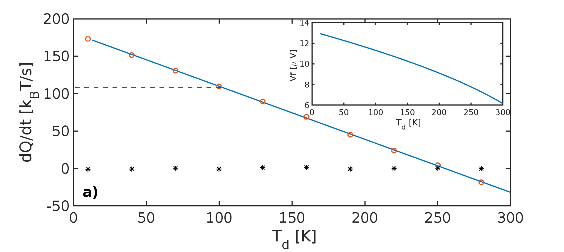
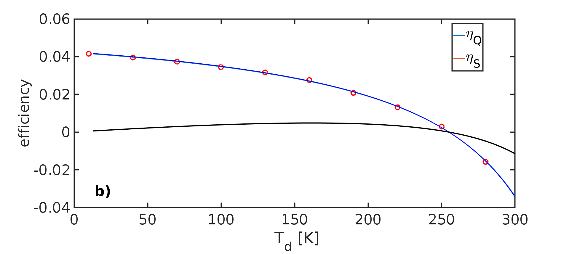
Figure 2: a) Heat fluxes as a function of the demon temperature $T_{d}$ :$\left<{\dot{Q}_{2}}\right>$ (blue line) computed when the demon is on, using eqs.13,..,16 and the condition for $V_{t}^{2}$ eq.19; $\left<{\dot{Q}_{1}}\right>$ (horizontal red dashed line) computed (eq.6) when the demon is ”off” ; $\left<{\dot{Q}_{2}}\right>$ (red circles) and $\left<{\dot{Q}_{2}}\right>+\left<{\dot{Q}_{1}}\right>$ (black stars) obtained from the direct numerical simulation of eqs.7,..,10. b) Demon efficiencies as a function of $T_{d}$: $\eta_{s}$ (black line) and $\eta_{Q}$ (blue line, red circles) computed from eqs.14,16,25 (continuos lines) and obtained from the direct numerical simulations of eqs.7,..,10 (red circles). The parameters used to compute the curves in a) and b) are: $T_{1}=300$K, $T_{2}=450$K,$C=1$nF, $C_{1}=C_{2}=100$pF, $R_{1}=R_{2}=10\rm{M}\Omega$;$R_{d}=3\rm{M}\Omega$;$Cd=50$pF.

However the demon produces entropy and the total entropy production rate $\left<{\dot{S}}\right>$ is positive in spite of the fact that the system entropy production rate
$\left<{\dot{S}_{s}}\right>=\left<{\dot{Q}_{2}}\right>\left({1}/{T_{2}}-{1}/{T_{1}}\right)$ is negative, because $\left<{\dot{Q}_{2}}\right>>0$ and $T_{2}>T_{1}$ when the demon is ”on”. The total entropy production rate is

$$\left<{\dot{S}}\right> = \frac{\left<{\dot{Q}_{d}}\right>}{T_{d}}+\left<{\dot{Q}_{2}}\right>\left(\frac{1}{T_{2}}-\frac{1}{T_{1}}\right)$$ (24)

To show that $\left<{\dot{S}}\right>>0$, we start by taking into account that $\left<{\dot{Q}_{d}}\right>=\left<{\dot{W}_{f}}\right>$ (see eq.18) and that $\left<{\dot{W}_{f}}\right>>{V_{t}^{2}\over R_{2}}$ because as we said ${V_{t}^{2}\over R_{2}}$ is a fraction of the total power injected into the system by the demon source (computed Appendix E). Furthermore as we want $\left<{\dot{Q}_{2}}\right>>0$ then from eq.14 we have that $V_{t}^{2}/R_{2}>\left<{\dot{Q}_{2}}\right>$ as the other terms are negative because $T_{2}>T_{1}>T_{d}$. As a consequence
$\left<{\dot{Q}_{d}}\right>/T_{d}>\left<{\dot{Q}_{d}}\right>(1/T_{1}-1/T_{2})>\left<{\dot{Q}_{2}}\right>(1/T_{1}-1/T_{2})$ and we find $\left<{\dot{S}}\right>>0$.

These results on the effect of the demon on the system can be checked by comparing the heat fluxes computed from eqs.13,14 with those obtained by the direct numerical integration of eqs.7-10, where the four $<\dot{Q}_{k}>=<v_{k}\dot{q}_{k}>$ are directly computed using Stratonovich integrals. This comparison is done using for the system components (i.e.$R_{1},R_{2},C_{1},C_{2},C$) the values of the experiment of ref.Ciliberto et al. (2013a, b). For the demon, we chose for $C_{d}$ a typical wiring value and we fixed $R_{d}<R_{2}$ for having a reasonable range of $T_{d}$ (see eq.20). All the components and temperatures values are indicated in the caption of fig.2. In fig.2a) the horizontal red dashed line indicates $|<\dot{Q}_{2}>|$ at $T_{2}-T_{1}=150$K computed from eq.6 when the demon is ”off”. When the demon is ”on” the value of $\dot{Q}_{2}$ computed from eqs.14 and that obtained from direct numerical simulation agree. Most importantly for $T_{d}<250$K the heat flows from the cold to the hot thermal bath. The values of $V_{t}$ necessary for implementing the demon conditions (eq.19) are plotted in the inset indeed for these values of $V_{t}$ we see that $<\dot{Q}_{2}>+<\dot{Q}_{1}>=0$ in the numerical simulation. It is important to notice that the necessary $V_{t}$ is of the order of a few microvolts meaning that it can be easily obtained by two thermocouples coupled with a cold and an hot bath for example $T_{1}$ and $T_{2}$.

The Demon efficiency can be defined in two ways. As the demon does not exchange any work and heat with the system then the efficiency can be defined in terms of entropy production rates, which has been used in other contexts Verley et al. (2014); Polettini et al. (2015); Derivaux and De Decker (2019). Another way to define efficiency is in terms of the energy fluxes. Specifically these efficiencies are :

$$\eta_{s}=-\ {\dot{S}_{s}\over\dot{S}_{d}}\ \ \rm{and}\ \ \eta_{Q}={<\dot{Q}_{2}>\over<\dot{W}_{f}>}.$$ (25)

We see that $\eta_{s}$ is the ratio between the entropy of the non spontaneous process divided by the entropy of the spontaneous process whereas $\eta_{Q}$ is the ratio between the reversed heat flux in the system divided by the work performed by the demon to achieve the goal. These two quantities are plotted in fig.2b) as function of $T_{d}$, and we observe that $\eta_{s}<1\%$ and $\eta_{Q}<4\%$, i.e. in order to achieve its goal the demon has to do a lot of work with a very large entropy production rate.

To conclude, we have simplified the original idea of autonomous OEMD because we use a demon with a single bath and a DC forcing (powered by thermocouples) instead of two baths with colored noise as in ref.Sanchez et al. (2019). We have demonstrated that this autonomous OEMD can be applied to electric circuits in order to reverse the spontaneous heat processes with no energy exchange between the system and demon. The latter has a small efficiency and a very large positive entropy production rate that largely compensates the negative entropy production rate of the system. Our results are very general because they are based on four coupled Langevin equations, which model not only electric circuits, but a lot of micro and nano-systems. Thus this article paves the way to the general applications of OEMDs to the control of these mesoscopic systems. We have chosen this configuration as a proof of principle but other complex circuits can of course be implemented.

Appendix A Several details about the demon

In this section we describe the out of equilibrium demon, composed by two resistances ($Rd_{1}$ and $Rd_{2}$) kept at two different temperatures $Td_{1}$ and $Td_{2}$. The two voltage generators $\eta d_{1}$ and $\eta d_{2}$ corresponding to the Nyquist noise of the two resistances at the temperatures of the heat baths. Furhermore the resistance Rd2 is driven by a voltage generator $V_{s}$ whose out-put is fltered by the the low pas filter composed by the resistance $Rs$ and the capacitance $C_{s}$.

A.1 The demon as a colored noise generator

The dynamics of the demon can be obtained by writing the Kirchhoff laws for the points $V_{f}$ and $V_{d}$ :

$${V_{s}-V_{f}\over R_{s}}-\dot{V}_{f}\ C_{f}-{V_{f}+\eta_{d2}-V_{d}\over R_{d2}} = 0$$ (26)

$${V_{f}+\eta_{d2}-V_{d}\over R_{d2}}-\dot{V}_{d}\ C_{d}-{V_{d}-\eta_{d1}\over R_{d1}}-i_{d} = 0$$ (27)

where $i_{d}$ is the current flowing between the system and the demon when the latter is ”on”. From these equations we get:

$$\tau_{f}\ \dot{V}_{f}=-V_{f}+{R_{f}\over R_{s}}V_{s}+{R_{f}\over R_{d2}}(V_{d}-\eta_{d2})$$ (28)

$$\tau_{d}\ \dot{V}_{d}=-V_{d}+\left({R_{d}\over R_{d2}}V_{f}-i_{d}\ R_{d}\right)+\xi_{d}$$ (29)

where we use :

$$R_{d} = {R_{d1}\ R_{d2}\over R_{d1}+R_{d2}},\ \ \tau_{d}=R_{d}C_{d},\ \ R_{f}={R_{s}\ R_{d2}\over R_{d2}+R_{s}},\ \ \ \ \tau_{f}=R_{f}C_{s}\ \ \ \rm{and}\ \ \ \ \xi_{d}=\eta_{d1}{R_{d}\over R_{d1}}+\eta_{d2}{R_{d}\over R_{d2}}.$$ (31)

As $V_{s}$ is not necessarily the thermal noise of $R_{s}$, it can be a very large external driving that allows the demon to work, we can simplify this circuit if we assume that $R_{d2}>>R_{s}$

$$\tau_{f}\ \dot{V}_{f} = -V_{f}+V_{s}$$ (32)

$$\tau_{d}\ \dot{V}_{d} = -V_{d}-\left({R_{d}\over R_{d2}}V_{f}-i_{d}\ R_{d}\right)+\xi_{d}$$ (33)

These equations show that the demon produces colored noise for the system as it is needed to control the system heat flux.

A.2 The heat flux in the demon switched off

When $V_{s}=0$ and $i_{d}=0$ the heat transfers between the two reservoirs of the demon can be obtained from eqs.6 for $C\rightarrow\infty$. Thus the heat transfers in the demon are:

$$\left<{\dot{Q}_{d1}}\right> = \frac{k_{B}(T_{d2}-T_{d1})}{(R_{d1}+R_{d2})C_{d}}.$$ (34)

$$\left<{\dot{Q}_{d2}}\right> = \frac{k_{B}(T_{d1}-T_{d2})}{(R_{d1}+R_{d2})C_{d}}.$$ (35)

When there is an external driving one has also to consider the work performed by the external source $V_{f}$ still in the case $i_{d}=0$,i.e. with the demon is not connected to the system. We can use for $Vs$ either thermal fluctuations of $Rs$ with a suitable cut-off imposed by the $R_{s}C_{s}$ or an external driving. In the simplest version we make the choice to use a $V_{f}=V_{s}$ constant and $Rs=0$. In such a case the heat dissipated by the two resistances is:

$$\left<{\dot{Q}_{d1}}\right> = \frac{k_{B}(T_{d2}-T_{d1})}{(R_{d1}+R_{d2})C_{d}}+{V_{f}^{2}R_{d1}\over(R_{d1}+R_{d2})^{2}}$$ (36)

$$\left<{\dot{Q}_{d2}}\right> = \frac{k_{B}(T_{d1}-T_{d2})}{(R_{d1}+R_{d2})C_{d}}+{V_{f}^{2}R_{d2}\over(R_{d1}+R_{d2})^{2}}$$ (37)

and doing the energy balance we have

$$\left<{\dot{Q}_{d1}}\right>+\left<{\dot{Q}_{d2}}\right>=\ {V^{2}\over(R_{d1}+R_{d2})}=\ \left<{\dot{W}_{f}}\right>$$ (38)

where $\left<{\dot{W}_{f}}\right>$ is the power injected into the demon by the voltage generator. where we use the convention that the heat dissipated in the bath and the work performed on the system are positive. Thus the demon is always out of equilibrium even at $T_{d1}=T_{d2}$

Appendix B The currents in the system+demon circuit

We now connect the demon to the system and this connection changes the current distributions. We write the equations of the circuits in terms of charges. The relationships between currents and charges are

$$0 = -\dot{q}_{1}-\dot{q}_{c1}+\dot{q}_{c},\ \ \ \dot{q}_{2}-\dot{q}_{ct}-\dot{q}c+\dot{q}_{d2}+\dot{q}_{d1}=0,$$

$$\dot{q}_{c} = (V_{2}-V_{1})C,\ V_{1}C_{1}=q_{c1}\ \rm{and}\ \ V_{2}C_{t}=q_{ct}$$ (39)

where $\dot{q}_{k}$ ($k=1,2,d1,d2$) are the currents flowing in the resistances $R_{k}$. Futhermore $\dot{q}_{c},\dot{q}_{c1}$ and $\dot{q}_{ct}$ are the currents flowing respectively in the capacitors $C,C_{1}$ and $C_{t}=C_{2}+C_{d}$. Solving the system for $q_{c1}$ and $q_{ct}$ we find :

$$V_{1}={q_{c1}\over C_{1}} = {-(C_{t}+C)\ q_{1}+\ C\ q_{t}\over X_{t}}$$ (40)

$$V_{2}={q_{ct}\over C_{t}} = {(C_{1}+C)\ q_{t}-\ C\ q_{1}\over X_{t}}$$ (41)

where $q_{t}=(q_{2}+q_{d2}+q_{d1})$ and $X_{t}=C_{1}C_{t}+C(C_{1}+C_{t})$. we can now solve for the four currents flowing in the 2 system resistances and the two demon resistances specifically

$$R_{1}\ \dot{q}_{1} = V_{1}-\eta_{1}={-(C_{t}+C)\ \ q_{1}+\ C\ (q_{2}+q_{d2}+q_{d1})\over X_{t}}-\eta_{1}$$ (42)

$$R_{2}\ \dot{q}_{2} = \eta_{2}-V_{2}={-(C_{1}+C)\ \ (q_{2}+q_{d2}+q_{d1})+\ C\ q_{1}\over X_{t}}+\eta_{2}$$ (43)

$$R_{d1}\ \dot{q}_{d1} = \eta_{d1}-V_{2}={-(C_{1}+C)\ \ (q_{2}+q_{d2}+q_{d1})+\ C\ q_{1}\over X_{t}}+\eta_{d1}$$ (44)

$$R_{d2}\ \dot{q}_{d2} = \eta_{d2}+V_{f}-V_{2}={-(C_{1}+C)\ \ (q_{2}+q_{d2}+q_{d1})+\ C\ q_{1}\over X_{t}}+\eta_{d2}+V_{f}$$ (45)

We write the equations for the charges because the connection with Brownian particles is straightforward ($q$ correspond to the dispacement). Furthermore it is more clear to understand the amount of work performed by the demon on the system and the amount of dissipated heats in the various reservoirs. As the resistances of the demon are just in parallel to $R_{2}$ the equations 42,.,45 can be reduced to:

$$R_{1}\ \dot{q}_{1} = -{(C_{t}+C)\over X_{t}}\ \ q_{1}+\ {C\over X_{t}}\ q_{t}-\eta_{1}$$ (46)

$$R_{t}\ \dot{q}_{t} = -{(C_{1}+C)\over X_{t}}\ \ q_{t}+\ {C\over X_{t}}\ q_{1}+\ \eta_{t}+\ V_{t}$$ (47)

where we define

$$q_{t} = (q_{2}+q_{d2}+q_{d1}),\ \ \ \ R_{t}=(1/R_{2}+1/R_{d2}+1/R_{d1})^{-1},\ \ \rm{and},$$

$$\ \ V_{t} = V_{f}\ R_{t}/R_{d2},\ \ \ \eta_{t}=(\eta_{2}/R_{2}+\eta_{d1}/R_{d1}+\eta_{d2}/R_{d2})R_{t}.$$ (48)

Using eqs.4,5 we can compute the heat and the work of the different parts of the circuit. We can also use eqs. 6 to compute the total heat exchanged between the reservoir at $T_{1}$ with the reservoirs of resistance $R_{2},R_{d1},R_{d2}$. Defining $T_{t}=R_{t}(T_{2}/R_{2}+T_{d1}/R_{d1}+T_{d2}/R_{d2})$ and $Y_{t}=R_{1}\ (C+C_{1})+R_{t}\ (C+C_{t})$, we get :

$$\left<{\dot{Q}_{1}}\right> = \frac{C^{2}k_{B}(T_{t}-T_{1})}{X_{t}Y_{t}}.$$ (49)

$$\left<{\dot{Q}_{t}}\right> = \frac{C^{2}k_{B}(T_{1}-T_{t})}{X_{t}Y_{t}}$$ (50)

where the contribution of the work performed by $V_{t}$ cancels out in the stationary regime (see appendix E). Eq. 49 can be decomposed in the various contributions to the heat fluxes from the three reservoir at $(T_{2},T_{d1}$ and $T_{d2})$ :

$$\left<{\dot{Q}_{1}}\right> = \frac{C^{2}k_{B}}{X_{t}Y_{t}}\left(\frac{R_{t}}{R_{2}}(T_{2}-T_{1})+\frac{R_{t}}{R_{d1}}(T_{d1}-T_{1})+\frac{R_{t}}{R_{d2}}(T_{d2}-T_{1})\right)$$ (51)

Appendix C Calculation of the heat fluxes

By the definition eq.5 the heat fluxes in the resistances $k=1,2,d1,d2$ are given by:

$$\left<{\dot{Q}_{k}}\right> = \left<{{v_{k}}{(v_{k}-\eta_{k})\over R_{k}}}\right>.$$ (52)

where ${v_{k}}=V_{k}-V_{f}\ \delta_{k,d2}$ (with $V_{d1}=V_{d2}=V_{2}$) is the potential difference on the resistance $R_{k}$. The mean values can be evaluated by using the Fourier transforms $\tilde{v_{k}}$ of $v_{k}$, which can be written as :

$$\left<{\dot{Q}_{k}}\right> = \int_{0}^{\infty}\Re\left\{{{\frac{\tilde{v}_{k}^{*}}{R_{m}}(\tilde{v}_{k}-\tilde{\eta}_{k})}}\right\}\ \frac{d\omega}{2\ \pi}.$$ (53)

To evaluate this integral we take into account that the spectral density of $\tilde{\eta}_{k}$ is $|\tilde{\eta}_{k}|^{2}=4k_{B}T_{k}R_{k}$ and that $\Re\left\{{\eta_{k}\ \eta_{k^{\prime}}^{*}}\right\}=0$ because different noise sources are uncorrelated We have already computed $\left<{\dot{Q}_{1}}\right>$ in eq.49 and eq.51 using the eqs.6. We need to estimate all the heat fluxes in the demon reservoirs and in the reservoir 2 by computing $V_{1}$ and $V_{2}$ given by eqs.40 and 41. Their values depend on $q_{1},q_{t}$ which can be computed solving the system of eqs.46 and 47 in Fourier space.

$$Z_{1}\ \tilde{q}_{1}-a\ \tilde{q}_{t} = -\tilde{\eta}_{1}$$ (54)

$$-a\ \tilde{q}_{1}+Z_{t}\ \tilde{q}_{t} = \tilde{\eta}_{t}+V_{t}\ \sqrt{2\pi}\delta(\omega)$$ (55)

where $Z_{1}=(C_{t}+C)/X_{t}+i\omega R_{1}$, $Z_{t}=(C_{1}+C)/X_{t}+i\omega\ R_{t}$ and $a=C/X_{t}$. We find

$$\tilde{q}_{1} = {-\tilde{\eta}_{1}\ Z_{t}+\eta_{t}a\over\mathrm{det}}$$ (56)

$$\tilde{q}_{t} = {\tilde{\eta}_{t}\ Z_{1}-\eta_{1}a\over\mathrm{det}}$$ (57)

$$\mathrm{det} = Z_{1}\ Z_{t}-a^{2}={(1-\omega^{2}R_{1}R_{t}X_{t})+i\omega\ Y_{t}\over X_{t}}$$ (58)

Inserting these Fourier transform in eqs.40 and 41, we get:

$$\tilde{V}_{1} = \frac{\tilde{\eta}_{1}[1+i\omega\ R_{t}(C_{t}+C)]+\ \tilde{\eta}_{t}\ i\omega R_{1}C}{X_{t}\ \mathrm{det}}$$ (59)

$$\tilde{V}_{2} = \frac{\tilde{\eta}_{t}[1+i\omega\ R_{1}(C_{1}+C)]+\ \tilde{\eta}_{1}\ i\omega R_{t}C}{X_{t}\ \mathrm{det}}+V_{t}\ \sqrt{2\pi}\delta(\omega)$$ (60)

We see that

$$|\tilde{V}_{1}|^{2} = \frac{|\tilde{\eta}_{1}|^{2}\left[{1+(\omega\ R_{t}(C_{t}+C))^{2}}\right]+|\tilde{\eta}_{t}|^{2}(\omega R_{1}C)^{2}}{(1-\omega^{2}R_{1}R_{t}X_{t})^{2}+(\omega\ Y_{t})^{2}}$$ (61)

$$|\tilde{V}_{2}|^{2} = \frac{|\tilde{\eta}_{t}|^{2}\left[{1+(\omega\ R_{1}(C_{1}+C))^{2}}\right]+|\tilde{\eta}_{1}|^{2}(\omega R_{t}C)^{2}}{(1-\omega^{2}R_{1}R_{t}X_{t})^{2}+(\omega\ Y_{t})^{2}}+V_{t}^{2}{2\pi}\delta(\omega)$$ (62)

$$\left<{V_{1}^{2}}\right> = \int_{0}^{\infty}|\tilde{V}_{1}|^{2}\frac{d\omega}{2\ \pi}=\frac{|\tilde{\eta}_{1}|^{2}(X_{t}R_{1}R_{t}+R_{t}^{2}(C_{t}+C)^{2}+|\tilde{\eta}_{t}|^{2}R_{1}^{2}C^{2}}{4Y_{t}X_{t}\ R_{1}\ R_{t}}$$ (63)

$$\left<{V_{2}^{2}}\right> = \int_{0}^{\infty}|\tilde{V}_{2}|^{2}\frac{d\omega}{2\ \pi}=\frac{|\tilde{\eta}_{t}|^{2}(X_{t}R_{1}R_{t}+R_{1}^{2}(C_{1}+C)^{2})+|\tilde{\eta}_{1}|^{2}R_{t}^{2}C^{2}}{4\ Y_{t}X_{t}\ R_{1}\ R_{t}}+V_{t}^{2}$$ (64)

where we used the integrals:

$$\int_{0}^{\infty}\frac{Y_{t}}{{(1-\omega^{2}R_{1}R_{t}X_{t})^{2}+(\omega\ Y_{t})^{2}}}\ \frac{d\omega}{2\ \pi}=\frac{1}{4}\ \ \ \rm{and}\ \ \ \int_{0}^{\infty}\frac{Y_{t}\ \omega^{2}}{{(1-\omega^{2}R_{1}R_{t}X_{t})^{2}+(\omega\ Y_{t})^{2}}}\ \frac{d\omega}{2\ \pi}=\frac{1}{4\ R_{1}R_{t}X_{t}}$$ (65)

We can now compute the other heat fluxes :

$$\tilde{\dot{Q}}_{2} = \Re\left\{{\tilde{V}_{2}^{*}\frac{(\tilde{V}_{2}-\tilde{\eta}_{2})}{R_{2}}}\right\}=\frac{|\tilde{V}_{2}|^{2}}{R_{2}}-\Re\left\{{\frac{|\tilde{\eta}_{2}|^{2}R_{t}[1-i\omega\ R_{1}(C_{1}+C)]\mathrm{det}}{{R_{2}}^{2}\ X_{t}|\mathrm{det}|^{2}}}\right\}=$$ (66)

$$= \frac{|\tilde{V}_{2}|^{2}}{R_{2}}-\frac{|\tilde{\eta}_{2}|^{2}\ R_{t}\left[{(1-\omega^{2}R_{1}R_{t}X_{t})+\omega^{2}Y_{t}\ R_{1}\ (C_{1}+C)}\right]}{{R_{2}}^{2}\ \left[{(1-\omega^{2}R_{1}R_{t}X_{t})^{2}+(\omega\ Y_{t})^{2}}\right]}$$

$$\left<{\dot{Q}_{2}}\right> = \int_{0}^{\infty}\tilde{\dot{Q}}_{2}\ \frac{d\omega}{2\ \pi}=$$ (67)

$$= \frac{|\tilde{\eta}_{t}|^{2}\ R_{2}\ (X_{t}R_{1}R_{t}+R_{1}^{2}(C_{1}+C)^{2})+R_{2}|\tilde{\eta}_{1}|^{2}R_{t}^{2}C^{2}-|\tilde{\eta}_{2}|^{2}R_{t}\ Y_{t}\ R_{1}\ (C_{1}+C)}{4\ R_{2}^{2}\ Y_{t}X_{t}\ R_{1}\ R_{t}}=$$

$$= \frac{(|\tilde{\eta}_{t}|^{2}\ R_{2}-|\tilde{\eta}_{2}|^{2}R_{t})\ R_{1}(X_{t}R_{t}+R_{1}(C_{1}+C)^{2})+R_{t}^{2}C^{2}(|\tilde{\eta}_{1}|^{2}R_{2}-|\tilde{\eta}_{2}|^{2}R_{1})}{4\ R_{2}^{2}\ Y_{t}X_{t}\ R_{1}\ R_{t}}+{V_{t}^{2}\over R_{2}}$$

$$= -\frac{k_{B}C^{2}}{X_{t}\ Y_{t}}(T_{2}-T_{1})\frac{R_{t}}{R_{2}}-k_{B}\frac{X_{t}R_{t}+R_{1}(C_{1}+C)^{2}}{X_{t}\ Y_{t}R_{2}}\left({R_{t}\over R_{d1}}(T_{2}-T_{d1})+{R_{t}\over R_{d2}}(T_{2}-T_{d2})\right)+{V_{t}^{2}\over R_{2}}$$

$$\tilde{\dot{Q}}_{d2} = \Re\left\{{(\tilde{V}_{2}^{*}-V_{f}\sqrt{2\pi}\delta(\omega))\frac{(\tilde{V}_{2}-\tilde{\eta}_{d2}-V_{f}\sqrt{2\pi}\delta(\omega))}{R_{d2}}}\right\}$$ (68)

$$= \frac{|\tilde{V}_{2}|^{2}}{R_{d2}}-\Re\left\{{\frac{|\tilde{\eta}_{d2}|^{2}R_{t}[1-i\omega\ R_{1}(C_{1}+C)]\mathrm{det}}{{R_{d2}}^{2}\ X_{t}|\mathrm{det}|^{2}}}\right\}+{V_{t}(V_{t}-V_{f})\over R_{d2}}2\pi\delta(\omega)=$$

$$= \frac{|\tilde{V}_{2}|^{2}}{R_{d2}}-\frac{|\tilde{\eta}_{d2}|^{2}\ R_{t}\left[{(1-\omega^{2}R_{1}R_{t}X_{t})+\omega^{2}Y_{t}\ R_{1}\ (C_{1}+C)}\right]}{{R_{d2}}^{2}\ \left[{(1-\omega^{2}R_{1}R_{t}X_{t})^{2}+(\omega\ Y_{t})^{2}}\right]}+{(V_{t}-V_{f})^{2}\over R_{d2}}2\pi\delta(\omega)$$

$$\left<{\dot{Q}_{d2}}\right> = \int_{0}^{\infty}\tilde{\dot{Q}}_{d2}\ \frac{d\omega}{2\ \pi}=$$ (69)

$$= \frac{|\tilde{\eta}_{t}|^{2}\ R_{d2}\ (X_{t}R_{1}R_{t}+R_{1}^{2}(C_{1}+C)^{2})+R_{d2}|\tilde{\eta}_{1}|^{2}R_{t}^{2}C^{2}-|\tilde{\eta}_{d2}|^{2}R_{t}\ Y_{t}\ R_{1}\ (C_{1}+C)}{4\ R_{d2}^{2}\ Y_{t}X_{t}\ R_{1}\ R_{t}}+{(V_{t}-V_{f})^{2}\over R_{d2}}=$$

$$= \frac{(|\tilde{\eta}_{t}|^{2}\ R_{d2}-|\tilde{\eta}_{d2}|^{2}R_{t})\ R_{1}(X_{t}R_{t}+R_{1}(C_{1}+C)^{2})+R_{t}^{2}C^{2}(|\tilde{\eta}_{1}|^{2}R_{2}-|\tilde{\eta}_{d2}|^{2}R_{1})}{4\ R_{d2}^{2}\ Y_{t}X_{t}\ R_{1}\ R_{t}}+{(V_{t}-V_{f})^{2}\over R_{d2}}=$$

$$= -A\ (T_{d2}-T_{1})\frac{R_{t}}{R_{d2}}-B\frac{R_{d}}{R_{d2}}\left({R_{2}\over R_{d1}}(T_{d2}-T_{d1})+(T_{d2}-T_{2})\right)+{(V_{t}-V_{f})^{2}\over R_{d2}}$$

$$\rm{where}$$

$$A = \frac{k_{B}C^{2}}{X_{t}\ Y_{t}}\ \ \ \rm{and}\ \ \ B=k_{B}\frac{R_{t}(X_{t}R_{t}+R_{1}(C_{1}+C)^{2})}{X_{t}\ Y_{t}R_{2}R_{d}}$$ (70)

Finally using the same method we get:

$$\left<{\dot{Q}_{d1}}\right> = -A\ (T_{d1}-T_{1})\frac{R_{t}}{R_{d1}}-B\frac{R_{d}}{R_{d1}}\left({R_{2}\over R_{d2}}(T_{d1}-T_{d2})+(T_{d1}-T_{2})\right)+{V_{t}^{2}\over R_{d1}}$$ (71)

Appendix D The work performed by the demon on the system

We follow refs. Ciliberto et al. (2013a, b) to compute the power injected by the demon on $R_{1}$ and $R_{2}$ with $R_{d1}=R_{d2}$ and $T_{d1}=T_{d2}$

$$\left<{\dot{W}_{d,1}}\right> = \frac{C}{X_{t}}\left<{\dot{q}_{1}\ (q_{d1}+q_{d2})}\right>=\int_{0}^{\infty}{\Re\left\{{{\tilde{V}_{1}^{*}-\tilde{\eta}_{1}^{*}\over R_{1}}\ {\tilde{\eta}_{d}-\tilde{V}_{2}\over R_{d}\ i\omega}}\right\}}{d\omega\over 2\pi}=$$ (72)

$$= -\frac{C}{X_{t}}\int_{0}^{\infty}\left[|\tilde{\eta}_{1}|^{2}R_{t}\ C-|\tilde{\eta}_{t}|^{2}R_{1}\ C+(1-\omega^{2}R_{1}\ R_{t}\ X_{t})R_{t}\ C\ (-|\tilde{\eta}_{1}|^{2}+|\tilde{\eta}_{d}|^{2}R_{1}/R_{d})\over R_{1}R_{d}|det|^{2}X_{t}^{2}\right]{d\omega\over 2\pi}=$$ (73)

$$= -k_{B}{C^{2}R_{t}\over X_{t}\ Y_{t}\ R_{d}}(T_{1}-T_{t})={A\ R_{t}^{2}\over\ R_{d}\ R_{2}}(T_{2}-T_{1})-{A\ R_{t}^{2}\over\ R_{d}^{2}}(T_{1}-T_{d})$$ (74)

where we used eqs59, 60, $T_{t}=R_{t}(T_{2}/R_{2}+T_{d}/R_{d})$ and eqs.70.

$$\left<{\dot{W}_{d,2}}\right> = -\frac{(C_{1}+C)}{X_{t}}\left<{\dot{q}_{2}\ (q_{d1}+q_{d2})}\right>=-\frac{(C_{1}+C)}{X_{t}}\int_{0}^{\infty}{\Re\left\{{{\tilde{\eta}_{2}^{*}-\tilde{V}_{2}^{*}\over R2}\ {\tilde{\eta}_{d}-\tilde{V}_{2}\over R_{d}\ i\omega}}\right\}}{d\omega\over 2\pi}+{V_{t}^{2}\over R_{2}}=$$ (75)

$$= -{(C_{1}+C)\over X_{t}\ R_{2}\ R_{d}}\int_{0}^{\infty}{({|\tilde{\eta}_{2}|^{2}R_{t}/R_{2}}-{|\tilde{\eta}_{d}|^{2}R_{t}/R_{d}})[Y_{t}-R1(C_{1}+C)(1-\omega^{2}R_{1}\ R_{t}\ X_{t})]\over X_{t}^{2}|det|^{2}}{d\omega\over 2\pi}+{V_{t}^{2}\over R_{2}}$$ (76)

$$= -k_{B}{(C_{1}+C)R_{t}\over X_{t}\ R_{2}\ R_{d}}(T_{2}-T_{d})+{V_{t}^{2}\over R_{2}}.$$ (77)

Adding a subtracting $A/R_{t}^{2}T_{1}/(R_{2}\ R_{d})$ from the last expression,taking into account the definition of $A$ and $B$ (eq.70), that $(C_{1}+C)(C_{t}+C)=X_{t}+C^{2}$ and that $k_{B}(C_{1}+C)R_{t}Y_{t}/(X_{t}\ R_{2}\ R_{d}Y_{t})=B+A/R_{t}^{2}/(R_{2}\ R_{d})$ we get

$$\left<{\dot{W}_{d,2}}\right> = -B\ (T_{2}-T_{d})-{A\ R_{t}^{2}\over R_{2}\ R_{d}}(T_{2}-T_{1})-{A\ R_{t}^{2}\over R_{2}\ R_{d}}(T_{1}-T_{d})+{V_{t}^{2}\over R_{2}}$$ (78)

The total work performed by the demon on the system is

$$\left<{\dot{W}_{d,s}}\right> = \left<{\dot{W}_{d,1}}\right>+\left<{\dot{W}_{d,2}}\right>=$$ (79)

$$= -A{R_{t}\over R_{d}}(T_{1}-T_{d})-B\ (T_{2}-T_{d})+{V_{t}^{2}\over R_{2}}$$ (80)

If the condition on the demon potential and temperature eqs.20 and 19 are satisfied then the last equation imposes that $\left<{\dot{W}_{d,s}}\right>=0$, i.e. the demon does not perform any work on the system.

Appendix E The power dissipated by the DC currents only

The power dissipated in the system and demon resistances by the DC external generator $V_{f}$ are:

$$P_{1} = 0,\ \ \ P_{2}=V_{t}^{2}/R_{2},\ \ \ P_{d1}=V_{t}^{2}/R_{d1},\ \ \ \ \ \ P_{d2}=(V_{f}-V_{t})^{2}/R_{d2}$$ (81)

with $V_{t}=\left<{V_{2}}\right>$. Taking into account that $V_{t}=V_{f}\ R_{t}/R_{d2}$ we get the total power supplied by the generator $V_{f}$

$$\left<{\dot{W}_{f}}\right>=P_{2}+P_{d1}+P_{d2}={V_{f}(V_{f}-V_{2})\over R_{d2}}$$ (82)

The dissipation of the demon is $P_{d}=P_{d1}+P_{d2}$ thus $P_{2}=\dot{W}_{d}-P_{d}$. This has been used in the text for computing the total entropy

Concerning the work of $V_{t}$ in eq.47 we clearly see that for the node 2, $\left<{\dot{q}_{t}}\right>=0$ if we consider only the DC current imposed by $V_{f}$. This means that $V_{t}\ \left<{\dot{q}_{t}}\right>=0$ and there is no contribution to the heat flux $\dot{Q}_{t}$ which is the heat exchanged by the equivalent $R_{t}$ circuit with the subsystem 1.