A comparative study of satellite galaxies in Milky Way-like galaxies from HSC, DECaLS and SDSS

Abstract

We conduct a comprehensive and statistical study of the luminosity functions (LFs) for satellite galaxies, by counting photometric galaxies from HSC, DECaLS and SDSS around isolated central galaxies (ICGs) and paired galaxies from the SDSS/DR7 spectroscopic sample. Results of different surveys show very good agreement. The satellite LFs can be measured down to $M_{V}\sim-10$, and for central primary galaxies as small as $8.5<\log_{10}M_{\ast}/M_{\odot}<9.2$ and $9.2<\log_{10}M_{\ast}/M_{\odot}<9.9$, which implies there are on average 3–8 satellites with $M_{V}<-10$ around LMC-mass ICGs. The bright end cutoff of satellite LFs and the satellite abundance are both sensitive to the magnitude gap between the primary and its companions, indicating galaxy systems with larger magnitude gaps are on average hosted by less massive dark matter haloes. By selecting primaries with stellar mass similar to our MW, we discovered that i) the averaged satellite LFs of ICGs with different magnitude gaps to their companions and of galaxy pairs with different colour or colour combinations all show steeper slopes than the MW satellite LF; ii) there are on average more satellites with $-15<M_{V}<-10$ than those in our MW; iii) there are on average 1.5 to 2.5 satellites with $M_{V}<-16$ around ICGs, consistent with our MW; iv) even after accounting for the large scatter predicted by numerical simulations, the MW satellite LF is uncommon at $M_{V}>-12$. Hence the MW and its satellite system are statistically atypical of our sample of MW-mass systems. In consequence, our MW is not a good representative of other MW-mass galaxies. Strong cosmological implications based on only MW satellites await additional discoveries of fainter satellites in extra-galactic systems. Interestingly, the MW satellite LF is typical among other MW-mass systems within 40 Mpc in the local Universe, perhaps implying the Local Volume is an under-dense region.

1 Introduction

In the structure formation paradigm of the $\Lambda$ cold dark matter ($\Lambda$CDM) scenario, galaxies form in the centres of an evolving population of dark matter haloes (White & Rees, 1978). Dark matter haloes grow in mass and size through both mergers with other haloes and the smooth accretion of diffuse matter (e.g. Wang et al., 2011a). Smaller haloes and their own central galaxies fall into larger haloes and become so-called “subhaloes” and “satellites” of the galaxy in the centre of the host halo.

Compared with the extra-galactic satellites around more distant central galaxies, the satellite galaxies in our Milky Way (hereafter MW) can be observed in great details. We are not only able to observe the MW satellites down to much fainter magnitudes, but also it is possible to measure their full 3-dimensional velocities as well as internal dynamics through observations of bright individual member stars. The MW system with its associated satellite galaxies thus offer an ideal environment to closely study satellite-properties, which, in turn, helps to probe the small mass end of galaxy formation, constrain the underlying dark matter distribution, and test the standard cosmological model on small scales.

With the observed abundance and properties of the MW satellites, a few so-called challenges to the standard cosmological model have been raised and are still under debates. The missing satellite problem (e.g. Klypin et al., 1999; Moore et al., 1999) is one example. Twenty years ago, it was pointed out that the observed number of satellite galaxies in the MW is significantly lower than the predicted number of dark matter subhaloes by numerical simulations. In the last decade, more faint satellite galaxies have been discovered in the Local Group (e.g. Irwin et al., 2007; Liu et al., 2008; Martin et al., 2008; Zucker et al., 2007; Watkins et al., 2009; Belokurov et al., 2010), but the number of observed satellites is still much smaller than the predicted number of subhaloes in cold dark matter simulations. To explain the problem, some studies invoke the model of warm dark matter, which predicts much less surviving small substructures (e.g. Lovell et al., 2014). On the other hand, this problem can be possibly explained by galaxy formation physics (e.g. Bullock et al., 2000; Benson et al., 2002a), such as photoionization and supernova feedback, which inhibit the star formation in small haloes, (e.g. Bullock et al., 2000; Benson et al., 2002a, b; Somerville, 2002), predicting that a significant number of small subhaloes do not host a galaxy. Moreover, it was estimated that there could be at least a factor of three to five times more faint satellites in the MW to be discovered (e.g. Koposov et al., 2008; Tollerud et al., 2008; Walsh et al., 2009; Hargis et al., 2014). More recently, with deep imaging surveys, more satellite galaxies or candidates in our MW and M31 are being discovered and reported (e.g. Bechtol et al., 2015; Drlica-Wagner et al., 2015; Kim et al., 2015; Koposov et al., 2015; Homma et al., 2018, 2019).

Another problem, known as the “too big to fail” problem, was raised by Boylan-Kolchin et al. (2011b). Our MW has nine classical dwarf spheroidal satellites that have maximum circular velocities, $V_{\mathrm{max}}$, smaller than 30 km/s. Only the Large and Small Magellanic Clouds (LMC and SMC) have $V_{\mathrm{max}}$ greater than 60 km/s, while the Sagittarius dwarf in our MW has $V_{\mathrm{max}}$ likely in between 30 and 60 km/s before infall. However, the most massive dark matter subhaloes predicted by $\Lambda$CDM simulations of MW-like systems are found to have $V_{\mathrm{max}}$ larger than those of MW satellites. It is thus hard to explain why the most massive subhaloes predicted by cold dark matter simulations do not match the properties of the most massive observed satellites. Proper mechanisms are required to explain how the central density of the most massive subhaloes in simulations can be reduced in order to match those of observed satellites, and such mechanisms include supernova feedback and subhalo disruption by the massive host halo (e.g. Garrison-Kimmel et al., 2019). Alternatively, the problem can be explained if the virial mass of our MW is smaller than that has been assumed. For example, Wang et al. (2012) and Cautun et al. (2014b) reported that the MW satellites are consistent with $\Lambda$CDM predictions at the 10% confidence level if the MW halo has a virial mass smaller than $1.3\times 10^{12}M_{\odot}$.

A lighter-mass MW-like halo, however, would have difficulties predicting the existence of the two massive satellite galaxies, LMC and SMC. They are very likely accreted by our MW, not as two individual satellites, but rather as a pair given their similarity in phase space (Kallivayalil et al., 2006), in good consistency with simulation results (e.g. D’Onghia & Lake, 2008). For galaxies with LMC stellar mass, the typical host halo mass is $\sim 2\times 10^{11}M_{\odot}$ before being accreted by a more massive host halo and becoming a satellite. The host halo mass of the SMC is approximately a factor of 2 to 3 smaller than that of the LMC. More recent studies suggest that the LMC could be as massive as $\sim 3\times 10^{11}M_{\odot}$ at infall (e.g. Cautun et al., 2019). Looking for subhaloes that are similar to the mass, Galactocentric distance, and the orbital velocity of the LMC in numerical simulations, Boylan-Kolchin et al. (2011a) concluded that the fraction of dark matter haloes smaller than $M_{200}\sim 1.25\times 10^{12}M_{\odot}$ hosting LMC-like subhaloes is very low ($<5\%$), and over 90% of haloes hosting LMC-like subhaloes have $M_{200}>1.7\times 10^{12}M_{\odot}$. In addition, although subhaloes with LMC or SMC-like masses are commonly found in MW-like haloes, it is rare to find MW-like haloes to host both LMC and SMC-like subhaloes. Only $\sim$2.5% of lighter-mass MW-like haloes with LMC analogous also have LMC-SMC pairs. Similar conclusions have been reached by, e.g., Busha et al. (2011); González et al. (2013) and Patel et al. (2017). In addition, Liu et al. (2011) looked at MW-MC-like systems in SDSS, and they claimed that galaxies with luminosity similar to the MW have only 3.5% probability of hosting both LMC and SMC-like satellites within a projected distance of 150 kpc.

The $V_{\mathrm{max}}$ distribution of classical satellites in our MW is also atypical. Cautun et al. (2014a) investigated the $V_{\mathrm{max}}$ distribution of massive subhaloes in MW-like hosts, by looking for haloes hosting at most three subhaloes with $V_{\mathrm{max}}\geq 30$km/s and at least two subhaloes with $V_{\mathrm{max}}\geq 60$km/s. They found that such cases are rare in $\Lambda$CDM simulations, with at most 1% of haloes of any mass having a similar distribution.

Thus, MW-like systems can be predicted and do exist in $\Lambda$CDM simulations, but some of the properties of the MW-system are statistically uncommon compared with simulated systems of similar central stellar mass or luminosity. However, we can not robustly rule out or claim challenges to the standard cosmology model with just the single case of our MW without determining statistical constraints on the properties of the satellite system. It is thus important to look at other extra-galactic satellites around MW-like galaxies, and investigate how differently the satellites in our MW are compared to the satellites of other galaxies. Such a comparative study can help to assess the statistical significance of previous cosmological implications based on MW satellites.

The MW satellite luminosity function can be measured down to $M_{V}\sim 0$ (e.g. Newton et al., 2018). The satellites of more distant extra-galactic galaxies, however, are more difficult to study to such faint magnitudes. In the very local universe (within $\sim$ 10 to 40 Mpc), efforts have been made to the detection and confirmation of faint satellites in other host galaxies. For example, Tanaka et al. (2018) investigated a few nearby MW-mass galaxies within $\sim$20 Mpc. With statistical background subtraction, their satellite luminosity functions can be measured down to $M_{V}\sim-9$, which show a large diversity. Carlsten et al. (2020a) measured the surface brightness fluctuation distances (e.g. Blakeslee et al., 2009; Cantiello et al., 2018; Carlsten et al., 2019) for dwarf satellites of 10 massive galaxies within 12 Mpc, and they reported that the MW satellite luminosity function is remarkably typical. Moreover, the SAGA (Satellites Around Galactic Analogs; Geha et al., 2017; Mao et al., 2020) survey measures the distribution of satellites around $\sim$100 MW-like systems within 40 Mpc, and the number of satellites per host shows large diversities. The MW satellite luminosity function is typical among these systems, though the satellites of MW and M31 were found to be redder than those in other MW-like systems within 40 Mpc.

In order to measure the intrinsic luminosities and distances of satellite galaxies beyond 40 Mpc and still at low redshifts, usually spectroscopic observations are required. However, spectroscopic surveys have bright flux limits, and thus studies based on pure spectroscopic data are often limited to a few brightest satellites. For example, the SAGA survey can reach $M_{V}\sim-12$ at the distance of 40 Mpc. At the redshift of $z\sim 0.1$, the distance is about 400 Mpc, corresponding to $\sim$5 magnitudes brighter than the limit at 40 Mpc.

Instead of looking at only spectroscopic companions, efforts have been devoted to measure the radial profiles and luminosity functions of photometric satellites around spectroscopic host galaxies at $z\sim 0.1$ (e.g. Lares et al., 2011; Wang et al., 2011b; Guo et al., 2011b; Wang & White, 2012; Jiang et al., 2012; Wang et al., 2014; Cautun et al., 2015; Lan et al., 2016; Tinker et al., 2019) and also to intermediate and high redshifts (e.g. Nierenberg et al., 2013; Kawinwanichakij et al., 2014), based on statistical background subtraction approaches to remove the contamination by foreground and background galaxies. The significantly fainter flux limits of photometric surveys can help to study satellites that are much fainter than those accessible by spectroscopic observations. Using the photometric catalogues of the Sloan Digital Sky Survey (SDSS), the satellite luminosity function of galaxies at $z\sim 0.1$ can be measured down to $M_{V}\sim-14$, which covers the bright end of MW satellites (e.g. Guo et al., 2011b; Wang & White, 2012).

More recently, there are a few on-going and future deep imaging surveys such as the DESI Legacy Imaging Survey (Dey et al., 2019), the Hyper Suprime-Cam Subaru Strategic Program (HSC; Aihara et al., 2018a) and the future Vera Rubin Observatory Legacy Survey of Space and Time (LSST; Ivezić et al., 2008). These surveys are promising to extend previous studies based on SDSS down to fainter magnitudes, though follow-up spectroscopic surveys are still required to identify central galaxies in their footprints. Fortunately, the on-going HSC survey and the DESI Legacy Imaging Survey (Dey et al., 2019) already have part of their footprints overlapping with the SDSS spectroscopic galaxies. In this study, we select central primary galaxies similar to the MW from the SDSS spectroscopic Main galaxy sample and investigate their satellite luminosity function (hereafter LF) using photometric sources from HSC and DECaLS (the Dark Energy Camera Legacy Survey). We also repeat the same analysis with SDSS imaging data, in order to cross check the consistency of our measurements in different surveys. We will show whether the LF of satellites in our MW is typical compared with the averaged satellite LF around extra-galactic central galaxies with similar properties.

The structure of this paper is organised as follows. We introduce how we select central primary galaxies and the photometric source catalogues of HSC, DECaLS and SDSS used to construct satellite galaxies in Section 2. Our methodology of satellite counting, background subtraction and the projection effect are described in Section 3. Results are presented in Section 4, for the measured satellite LFs centred on primary galaxies selected in many different ways. We discuss and conclude in the end (Sections 5 and 6).

For observational results, we adopt the first-year Planck cosmology (Planck Collaboration et al., 2014) as our fiducial cosmological model, with the values of the Hubble constant $H_{0}=67.3\ \mathrm{km~{}s^{-1}/Mpc}$, the matter density $\Omega_{m}=0.315$ and the cosmological constant $\Omega_{\Lambda}=0.685$.

2 data

In order to investigate the extra-galactic satellite LFs, we need to first select samples of primary galaxies that sit in the centre of dark matter haloes. We make the selection in a few different ways. In brevity, we select isolated central galaxies that are brighter than or brighter by at least 1 magnitude than all companions. Then, we select galaxy pairs similar to our Local Group system. These primary galaxies are selected from the SDSS spectroscopic Main galaxy sample (Blanton et al., 2005), and the satellite counts are made from the photometric galaxies in either the HSC, DECaLS and SDSS footprints. In the following, we introduce how we select central primaries and the photometric source catalogues of different surveys used to construct satellites.

2.1 Isolated central galaxies

To identify a sample of primary galaxies that are highly likely sitting in the centre of dark matter haloes (purity), we select the brightest galaxies within given projected and line-of-sight distances. The parent sample used for the selection is the NYU Value Added Galaxy Catalogue (NYU-VAGC; Blanton et al., 2005), which is based on the spectroscopic Main galaxy sample from the seventh data release of the Sloan Digital Sky Survey (SDSS/DR7; Abazajian et al., 2009). The sample includes galaxies in the redshift range between $z=0.001$ and $z\sim 0.4$, which is flux limited down to an apparent magnitude of $\sim$17.7 in SDSS $r$-band, with most of the objects below redshift $z=0.25$. Stellar masses in VAGC were estimated from the K-corrected galaxy colours by fitting the stellar population synthesis model (Blanton & Roweis, 2007) assuming a Chabrier (2003) initial mass function.

We adopt two different sets of isolation criteria: i) Galaxies that are the brightest within the projected virial radius, $R_{200}$, of their host dark matter haloes and within three times the virial velocity along the line of sight. ii) Galaxies that are at least one magnitude brighter than all companions projected within the virial radius and within three times the virial velocity along the line of sight. In addition, galaxies selected in i) and ii) should not be within the projected virial radius (also three times virial velocity along the line of sight) of another brighter galaxy.

The SDSS spectroscopic sample suffers from the fiber-fiber collision effect that two fibers cannot be placed closer than 55$\arcsec$. As a result, galaxies in dense regions, such as those within galaxy groups and clusters, are spectroscopically incomplete. Moreover, for criterion ii), the companions used for the selection of isolated central galaxies fainter than $r=16.7$ can be fainter than the flux limit of the SDSS spectroscopic sample ($r=17.7$), and thus do not have spectroscopic redshift measurements. Hence to avoid the case when a galaxy has a brighter companion but this companion does not have available redshift and is hence not included in the SDSS spectroscopic sample, we use the SDSS photometric catalogue to make further selections. The photometric catalogue is the value-added Photoz2 catalogue (Cunha et al., 2009) based on SDSS/DR7, which provides photometric redshift probability distributions of SDSS galaxies. We further discard galaxies that have a photometric companion satisfying the magnitude requirement, whose redshift information is not available but is within the projected separation of the above selection criterion, and the photoz probability distribution of the photometric companion gives a larger than 10% of probability that it shares the same redshift as the central galaxy.

By adopting the flux limit of $r=17.7$ for primaries might induce a luminosity bias in the analysis, because when the selection is made near the faint limit of the spectroscopic sample, the faintest primaries will only have photometrically-identified companions. To ensure that our selection does not include any additional bias, we have explicitly repeated our analysis in this paper by adopting a flux limit of $r<16.7$ for primaries, so that all companions used for the selection of isolated central galaxy are above the flux limit of SDSS spectroscopic observations. Except for one of the conclusions which we will discuss in Section 5.2, all the other conclusions of this paper is robust against changes in the flux limit of central primaries.

Throughout the paper, primaries selected by adopting criteria i) and ii) are referred as ICG1 and ICG2 correspondingly. ICG1s are only mildly isolated. As tested against a mock galaxy catalogue based on the semi-analytical model of Guo et al. (2010), the completeness of ICG1s among all true halo central galaxies is above 90%. The purity is above 85%, which reaches $>$90% at $\log_{10}M_{\ast}/M_{\odot}>11.5$. The readers can check more details in Figure 2 of Wang et al. (2019). ICG2s are more strongly isolated, with a larger magnitude gap (at least one magnitude) to the companions. Thus, the completeness of ICG2s is lowered to between 60% and 70% at $\log_{10}M_{\ast}/M_{\odot}>11.2$, between 70% and 80% at $10.8<\log_{10}M_{\ast}/M_{\odot}<11.2$, between 80% and 90% at $10<\log_{10}M_{\ast}/M_{\odot}<10.8$ and is still above 90% at the small mass end. The purity fraction slightly increases to above 87%, which reaches $>$95% at $\log_{10}M_{\ast}/M_{\odot}>11.5$. The purity and completeness fractions predicted by the Illustris TNG-100 simulation (Nelson et al., 2019) are similar though noisier. The comparison between results based on ICG1s and ICG2s will help to determine whether the magnitude gap between the central primary and the companions can affect the satellite LF.

In this study, we will calculate the LF for satellites projected within the halo virial radius of ICGs. Instead of using the abundance matching formula to estimate $R_{200}$ for each individual ICG in a given stellar mass bin, we adopt the mean $R_{200}$ based on ICG1s selected from the mock galaxy catalogue of Guo et al. (2011a). Note the $R_{200}$ of ICG2s and primaries in pairs (see the next subsection) can be a bit different, but to ensure fair comparisons, we adopt the same $R_{200}$ for central primaries selected in different ways. The values of $R_{200}$ in these different bins are provided in Table LABEL:tbl:r200. In addition, we will also choose a stellar mass bin of $10.63<\log_{10}M_{\ast}/M_{\odot}<10.93$ for primaries with stellar mass similar to our MW (Licquia & Newman, 2015), and for this particular bin, we fix its virial radius to be 260 kpc. The choice of 260 kpc is motivated by the distance of Leo I (see Table LABEL:tbl:MWsat), and the virial radius of MW-mass ICG1s in the mock galaxy catalogue of Guo et al. (2011a) is close to 260 kpc. Table LABEL:tbl:r200 also provides the total number of ICG1s and ICG2s in each bin. Note the numbers of central primary galaxies in HSC are more than 10 times smaller, while the numbers of primaries in SDSS are slightly more than 50% the numbers in DECaLS due to better overlap, as primaries are selected from the SDSS spectroscopic Main galaxy sample. We avoid repeatedly showing the numbers of primaries in the footprints of all the three surveys.

Table 1: The average halo virial radii ($R_{200}$) for primary galaxies grouped by stellar mass, which are estimated using ICG1s selected from a mock galaxy catalogue of Guo et al. (2011). In each stellar mass bin, the numbers of ICG1s and ICG2s in the DECaLS footprint are provided.

$\log M_{\ast}/M_{\odot}$	$R_{\mathrm{200}}$ [kpc]	$N$ of ICG1	$N$ of ICG2
11.4-11.7	758.65	10188	3785
11.1-11.4	459.08	39621	19649
10.8-11.1	288.16	73755	49509
10.5-10.8	214.80	75366	59374
10.2-10.5	173.18	50795	43066
9.9-10.2	142.85	27873	24545
9.2-9.9	114.64	26919	24523
8.5-9.2	82.68	9787	9037
10.63-10.93	260.00	79840	59537

2.2 Galaxy pairs

Our MW has a massive companion, M31. The separation between the MW and M31 is $\sim$700 to 800 kpc. The virial radius of our MW is estimated to be in between 200 and 300 kpc in most previous studies(e.g. Gnedin et al., 2010; Eadie et al., 2015). We have introduced how the sample of ICGs are selected above. ICG1s have high completeness. They are more representative of the whole population of halo central galaxies and can contain galaxy pairs like our Local Group system. ICG1s can thus help to investigate the satellite LF around a general population of halo central galaxies. On the other hand, the more strictly selected ICG2s are at least one magnitude brighter than all companions within the virial radius, and thus the magnitude gap between ICG2s and their satellites is more comparable to the condition of our MW. Galaxy pairs like the MW and M31 can be included in the sample of ICG2s as well. In addition to ICG1s and ICG2s, here we also select a sample of galaxy pairs analogous to our MW and M31, in order to investigate whether their satellites have different LFs than ICGs and whether the satellite LFs depend on the properties of the other massive companion galaxy in the pair.

For galaxies with $10.2<\log_{10}M_{\ast}/M_{\odot}<11.1$ from the NYU Value Added Galaxy Catalogue, we identify pairs whose projected separations are in between twice the virial radius, $R_{200}$, of the more massive galaxy in the pair and 1,500 kpc. The line-of-sight distances are required to be smaller than seven times the mean virial velocity of the two galaxies in the pair. We require the mass ratio (large versus small value) of galaxies in the pair should be less than a factor of two. In addition, centred on the middle point of the two galaxies, all other companions projected within 800 kpc, and within seven times the virial velocity of the more massive primary galaxy along the line of sight, should be at least one magnitude fainter than the fainter primary galaxy in the pair. The SDSS photometric catalogue with photo-$z$ probability distributions (Cunha et al., 2009) is adopted for further selections as well, in order to compensate missing brighter companions due to fiber-fiber collisions.

In this paper, we will pick up galaxies in such pairs whose stellar masses are in the range of $10.63<\log_{10}M_{\ast}/M_{\odot}<10.93$, i.e., sharing a similar stellar mass range as our MW. However, when computing satellite counts around a given galaxy in a pair whose stellar mass is in this range, we choose not to make requirements on the stellar mass of its companion. In other words, though the stellar mass ratio between the two galaxies in the pair is less than a factor of two (sharing similar stellar mass), the stellar mass of the companion might still be out of the range of $10.63<\log_{10}M_{\ast}/M_{\odot}<10.93$. Our choice helps to maximise the available sample size. Besides, in this study we will investigate paired galaxies with different colour or colour combinations. We divide galaxies into red and blue populations by drawing a colour division line of ${}^{0.1}(g-r)=0.065\log_{10}M_{\ast}/M_{\odot}+0.1$ over the colour-magnitude diagram of SDSS spectroscopic galaxies. The number of red and blue primary galaxies in pair with $10.63<\log_{10}M_{\ast}/M_{\odot}<10.93$ are 893 and 738, respectively. The numbers of galaxies in red-red, blue-blue and red-blue pairs are 524, 341 and 766, respectively. Note the global colour of our MW very likely lies on this colour division line or in the green valley region, which we will discuss later in Section 5.

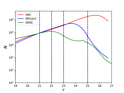
Figure 1: Number counts of all photometric sources in HSC, DECaLS and SDSS, as functions of $r$-band apparent magnitudes. Vertical dashed lines mark a few typical values of apparent magnitudes, i.e., $r=21,22,23$ and 24.

2.3 HSC photometric sources

The HSC survey (Aihara et al., 2018a) is based on the prime-focus camera, the Hyper Suprime-Cam (Miyazaki et al., 2012, 2018; Komiyama et al., 2018; Furusawa et al., 2018) on the 8.2-m Subaru telescope. It is a three-layered survey, aiming for a wide field of 1,400 deg² with a depth of $r\sim 26$, a deep field of 26 deg² with a depth of $r\sim 27$ and an ultra-deep field of 3.5 deg² with one magnitude fainter. In this work we use the wide field data. HSC photometry covers five bands, namely HSC-$grizy$. The transmission and wavelength range for each of the HSC $gri$-bands are almost the same as those of SDSS (Kawanomoto et al., 2018).

The HSC data reduction pipeline is an specialised version of the LSST (Jurić et al., 2017; Ivezić et al., 2019) pipeline code. Details about the HSC pipeline are available in the pipeline paper (Bosch et al., 2018), and we just briefly introduce the main steps in the following.

Data reduction is at first achieved on individual exposure basis. The sky background is estimated and subtracted before source detections, and the detected sources are used to calibrate the zero point and a gnomonic world coordinate system for each CCD by matching to external SDSS and Pan-STARRS1 (PS1; Schlafly et al., 2012; Tonry et al., 2012; Magnier et al., 2013; Chambers et al., 2016) sources. A secure sample of non-blended stars are used to construct the PSF model. Then a step called joint calibration is run to refine the astrometric and photometric calibrations, requiring that the same source appearing on different locations of the focal plane during different visits should give consistent positions and fluxes (Bosch et al., 2018). The HSC pipeline then resamples images to the pre-defined output skymap using a 5th-order Lanczos kernel(e.g. Jee & Tyson, 2011; Turkowski, 1990). All resampled images are combined together (coaddition).

From the coadd images, objects are detected, deblended and measured. A maximum-likelihood detection algorithm is run independently on the coadd image for each band. Background is estimated and subtracted in this step once again. The detected footprints and peaks of sources are merged across different bands to remove spurious peaks and maintain detections that are consistent over different bands. These detected peaks are deblended and a full suite of source measurement algorithm is run on all objects, yielding independent measurements of position and source parameters in each band. A reference band of detection is then defined for each object based on both the signal-to-noise and the purpose of maximising the number of objects in the reference band. Finally, the measurements of sources are run again with the position and shape parameters fixed to the values in the reference band to achieve the “forced” measurements, which brings consistency across bands and enables computing object colours using the magnitude difference in different bands.

In this paper, we use detected photometric galaxies from the S19A internal data release. The HSC database provides the extendedness flag to classify whether a detected source is more likely to be a point source or an extended galaxy. We thus use primary sources which are classified as extended. The type of magnitude for these extended HSC sources is the so-called cModel magnitude, based on fitting composite model combining Exponential and de Vaucouleurs profiles to source images. We exclude sources with any of the following pixel flags set as true in $g$, $r$ and $i$-bands: bad, crcenter, saturated, edge, interpolatedcenter or suspectcenter. We also limit ourselves to footprints which have reached full depth in $g$ and $r$-bands, i.e., number of exposures in $g$ and $r$ greater than or equal to four. The S19A bright star masks are created based on stars from Gaia DR2, and sources within the ghost, halo and blooming masks of bright stars in $i$-band have been excluded. The total area is a bit more than 450 square degrees.

As shown by Figure 1, the number counts of HSC sources keep rising to $r\sim 25$. In fact, as have been pointed out by Aihara et al. (2018b), the completeness of photometric sources in HSC is very close to 1 at $r\sim 25$. Thus throughout this paper, unless otherwise specified, we adopt a flux limit of $r<25$ for HSC photometric galaxies. However, also according to Aihara et al. (2018b), the quality of star-galaxy separation is very good at $r\sim 23$, but the completeness fraction of galaxies can drop to as low as 60–70% at $r\sim 25$, which depends on seeing. Note we do not worry about cases when stars are mis-classified as galaxies, because stars are not correlated with our sample of central primary galaxies, and thus are not expected to bias our results, though the contamination by stars might increase the level of foreground contamination and hence make the results noisier. On the other hand, if galaxies are mis-classified as stars, our results might be affected. Hence for results based on HSC in this study, we will also try a few different cuts in flux, including $r<21$, $r<23$ and $r<25$, to ensure the robustness of our results.

2.4 DECaLS photometric sources

The DESI Legacy Imaging Surveys are imaging the sky in three optical bands ($g$, $r$ and $z$) and four infrared bands, which comprise 14,000 deg² of sky area, bounded by $-18\deg<\mathrm{Dec.}<84\deg$ in celestial coordinates and $|b|>18\deg$ in Galactic coordinates (Dey et al., 2019). The surveys are comprised of 3 imaging projects, the Beijing-Arizona Sky Survey (BASS; Zou et al., 2017), the Mayall $z$-band Legacy Survey (MzLS) and the Dark Energy Camera Legacy Survey (DECaLS). The survey footprints are observed at least once, while most fields are observed twice or more times. In fact, the depth varies over the sky. In this paper, we mainly focus on the sky region with $\mathrm{Dec.}<33\deg$, i.e., the DECaLS footprint, which covers $\sim$9,000 deg². This southern footprint also includes data from the Dark Energy Survey (DES; Rossetto et al., 2011), which covers $\sim$5,000 deg² and is based on the same instrument as DECaLS, i.e., the Dark Energy Camera (DECam; Flaugher et al., 2015) at the 4-m Blanco telescope at the Cerro Tololo Inter-American Observatory.

Data used in this study are downloaded from the eighth data release of the DESI Legacy surveys. All data from the Legacy Surveys are first processed through the NOAO Community Pipelines (Dey et al., 2019). Briefly, after processing raw CCD images, the astrometric calibration is achieved against sources with known coordinates from external reference star samples. The world stars are from Gaia DR1 for data releases made later than the third release of the DESI Legacy surveys. A word coordinate system is determined for each CCD using these reference stars. The photometric calibration is based on PS1 DR1 sources. The zero point for each CCD is determined independently.

The photometric source product is constructed by tractor. tractor generates an inference-based model of the sky which best fits the real data. Here we briefly introduce the main post-processing steps. Basically, the survey footprint is divided into 0.25$\times$0.25$\deg^{2}$ regions, which is referred to as “bricks”. For a given brick, all CCDs overlapping with it can be found, and for each CCD, an initial sky background is estimated without masking sources. After subtracting the initial sky, sources are detected and masked, and the sky background is estimated again based on remaining pixels. The PSF for each CCD is determined using PSFEx (Bertin, 2011). Five independent stacks using sky subtracted and PSF convolved CCD images are then made for source detections, which include weighted sums of all CCDs in $g$, $r$ and $z$-bands, i.e., a weighted sum of all three bands to optimise a “flat” SED with zero AB magnitude colour and a weighted sum of all three bands to optimise a “red” SED with $g-r=1$ and $r-z=1$. Sources are then detected using the five stacks with a threshold of $6\sigma$. For each detected source, tractor models its pipeline-reduced images from different exposures and in multiple bands simultaneously. This is achieved by fitting parametric profiles including a delta function (for point sources), a de Vaucouleurs law, an exponential model or de Vaucouleurs plus exponential to each image simultaneously. The model is assumed to be the same for all images and is convolved with the corresponding PSF in different exposures and bands before fitting to each image. The best fit is achieved by minimising the residuals of all images. tractor also outputs the quantity which can be used to distinguish extended sources (galaxies) from point sources (stars).

Starting from the DESI Legacy Survey database sweep files, we remove all sources with TYPE classified as “PSF”, and require BITMASK not containing any of the following: BRIGHT, SATUR_G (saturated), SATUR_R, SATUR_I, ALLMASK_G, ALLMASK_R, ALLMASK_I. According to Figure 1, the average number counts of DECaLS sources keep rising to $r\sim 23$. However, given the variation of the depth over the sky, unless otherwise specified, we adopt a flux cut of $r<22.5$ to define a safe flux limited sample throughout our analysis in this study. We only use the regions with depth deeper than 22.5 in $r$. This is achieved by at first selecting bricks with at least three exposures in both $g$ and $r$-bands, and we also require the $r$-band GALdepth of the bricks to be deeper than 22.5. We only include galaxies within these selected bricks. For each galaxy, its GALdepth is additionally required to be deeper than $r=22.5$, otherwise this galaxy is excluded. In addition, to ensure the robustness of our results, we will test another two different choices of flux limits, $r<21$ and $r<23$. For DECaLS, the completeness of objects classified as extended galaxies is above 90% at $r<22.5$.

2.5 SDSS photometric sources

SDSS used a dedicated wide-field 2.5m telescope (York et al., 2000; Gunn et al., 2006) to image the sky in the drift scan mode with five optical filters, $ugriz$ (Fukugita et al., 1996; Gunn et al., 1998). The sample of SDSS photometric galaxies used to construct satellite counts in this study is exactly the same as those used in Wang & White (2012) and Wang et al. (2014). As have been discussed extensively in the Appendix of Wang & White (2012), by using internal tests based on the data itself, external tests using mock catalogues based on both directly projecting the simulation box and light-cone mocks considering a series of realistic observational effects, the measured satellite luminosity and stellar mass functions are robust against sample completeness, star-galaxy separation, projection effects, background subtraction and K-corrections. In this study, we repeat our analysis with our new primaries, and we will make detailed comparisons among results based on SDSS, DECaLS and HSC, to validate the robustness of our results based on surveys with different observing strategy, data reduction, resolution and depth.

The sample of photometric galaxies is downloaded from Casjobs of SDSS DR8. Specifically, we downloaded sources which are classified as galaxies in the survey’s primary object list, and that do not have any of the flags: BRIGHT, SATURATED, SATURCENTER or NOPETROBIG set. This follows the selection for the DR7 photoz2 catalogue used above when selecting primary galaxies. SDSS DR8 has included an improved algorithm of background subtraction than previous releases, and has eliminated the number of spurious sources which exist in DR7 (e.g. Mandelbaum et al., 2005; Aihara et al., 2011). We only use the sources within the acception masks of the DR7 VAGC catalogue, which are stored as spherical polygons. Note using later data releases will not increase the signal, because our spectroscopic primary galaxies are selected from the DR7 Main galaxies, and the overlapping footprints with releases later than DR8 are not increased. Throughout the paper, we use the Petrosian magnitude for SDSS, which self-consistently defines the colour of galaxies within the same aperture size crossing different bands. The flux limit we adopt for SDSS is the same as Wang & White (2012), i.e., $r<21$. As the readers can also see from Figure 1, number counts of SDSS sources keep rising to $r\sim 21$, and as has been shown in the Appendix of Wang & White (2012), the completeness of SDSS extended galaxies is very close to 1 above this flux limit.

Table 2: Galactocentric positions and $V$-band absolute magnitudes of six MW satellites brighter than $M_{V}\sim-10$. Riley et al. (2019) defined the spherical coordinate system in the following way. The $x$-axis points from the Sun to the Galactic centre, the $y$-axis points towards the direction of Galactic longitude, $l=90$ deg, and the $z$-axis points towards the north Galactic pole. $\theta$ is defined from the $z$-axis, and $\phi$ is defined from the $x$-axis so that the Galactic rotation is in the $-\phi$ direction.

Satellite	$r_{\mathrm{GC}}$ [kpc]	$\theta$ [deg]	$\phi$ [deg]	$M_{V}$
Sagittarius I	$18.3_{-2.0}^{+2.0}$	$110.6_{-0.6}^{+0.8}$	$8.2_{-0.3}^{+0.3}$	$-$13.5
LMC	$50.3_{-1.9}^{+2.0}$	$123.3_{-0.0}^{+0.0}$	$-90.7_{-0.5}^{+0.4}$	$-$18.1
SMC	$61.3_{-3.8}^{+4.2}$	$136.9_{-0.1}^{+0.1}$	$-66.8_{-0.7}^{+0.6}$	$-$16.8
Sculptor	$84.0_{-1.5}^{+1.5}$	$172.5_{-0.1}^{+0.1}$	$-119.7_{-0.1}^{+0.9}$	$-$11.1
Fornax	$149.5_{-9.0}^{+8.6}$	$153.9_{-0.1}^{+0.1}$	$-129.1_{-0.4}^{+0.3}$	$-$13.4
Leo I	$261.9_{-9.3}^{+9.2}$	$41.7_{-0.0}^{+0.0}$	$-135.8_{-0.1}^{+0.1}$	$-$12.03

2.6 Milky Way satellites

The $V$-band luminosity, R.A., Dec. and distances of the MW satellites are taken from Newton et al. (2018), Riley et al. (2019) and Li et al. (2020). As the readers will see, the MW satellites which can be used to compare with extra-galactic satellites from HSC, DECaLS and SDSS photometric sources introduced above are all brighter than $M_{V}\sim-10$. These include LMC, SMC, Fornax, Leo I, Sculptor and Sagittarius-I. We provide in Table LABEL:tbl:MWsat the Galactocentric distances, positions and $V$-band absolute magnitudes of these satellites.

2.7 Illustris TNG-100 and L-Galaxies

We will use the hydro-dynamical Illustris TNG-100 simulation, and the L-Galaxies semi-analytical mock galaxy catalogue to aid our analysis. In the following we briefly introduce them.

The TNG series of simulations include a comprehensive model for galaxy formation under the standard cosmological context. The fiducial cosmological parameters are the 2015 Planck cosmology (Planck Collaboration et al., 2016) ($H_{0}=67.74\ \mathrm{km~{}s^{-1}/Mpc}$, $\Omega_{m}=0.3089$ and $\Omega_{\Lambda}=0.6911$). It self-consistently solves for the coupled evolution of dark matter, gas, stars, and black holes from early times to $z=0$ (Nelson et al., 2019; Marinacci et al., 2018), which produced reasonable and quantitative agreement with the colour distribution, clustering, satellite abundance and stellar mass distribution of observed galaxies (e.g. Nelson et al., 2018; Springel et al., 2018; Pillepich et al., 2018). The box size of TNG-100 is 75 $h^{-1}$Mpc, and the particle mass of dark matter is $7.5\times 10^{6}M_{\odot}$, which corresponds to a resolution limit of about $7.5\times 10^{8}M_{\odot}$ in halo mass. The satellite LFs of TNG-100 tend to be incomplete beyond $M_{V}\sim-16$ due to the resolution limit.

The semi-analytical galaxy formation code, L-Galaxies, describes the physical processes of galaxy formation analytically, by tracing the halo merger histories of the Millennium (Springel et al., 2005) and Millennium-II (Boylan-Kolchin et al., 2009) simulations. The 2015 L-galaxies mock galaxy catalogue (Henriques et al., 2015) rescales (Angulo & White, 2010) the original simulation to the first-year Planck cosmology (Planck Collaboration et al., 2014) ($H_{0}=67.3\ \mathrm{km~{}s^{-1}/Mpc}$, $\Omega_{m}=0.315$ and $\Omega_{\Lambda}=0.685$). Compared with early versions of the Munich semi-analytical models (Guo et al., 2011a, 2013), it has included a few modifications in the treatment of baryonic processes, in order to reproduce observations on the abundance and passive fractions of galaxies from $z=3$ to $z=0$. In this study, we use the L-Galaxies mock galaxy catalogue based on Millennium-II, which has a higher resolution limit than Millennium, a simulation box size of 100 $h^{-1}$Mpc, and the dark matter particle mass of $6.9\times 10^{6}h^{-1}M_{\odot}$. In addition, L-Galaxies models the evolution of orphan galaxies whose dark matter haloes have been entirely disrupted, by tracing the most bound dark matter particles after disruption. Over the luminosity range probed in this paper ($M_{V}<-10$), the L-Galaxies satellite LFs based on Millennium-II agree well with real observations.

3 Methodology

3.1 Satellite luminosity function

Our methods of counting photometric satellites around spectroscopic primary galaxies and computing the intrinsic luminosities of satellites are based on the approach of Wang & White (2012). For each primary galaxy in a given stellar mass bin, we at first count all its photometric companion galaxies down to a certain flux limit and projected within the halo virial radius, $R_{200}$ (see Table LABEL:tbl:r200). The physical scale is calculated based on the redshift and angular diameter distance of the central primary. However, without redshift information and accurate distance measurements for these photometric companions, the companion counts can only be recorded as a function of apparent magnitude and observed-frame colour. In addition, the total companion counts not only include true satellites, but also include contamination by fore/background sources.

We obtain the intrinsic luminosities and rest-frame colours for companions in the following way. For each companion, we employ the empirical K-correction of Westra et al. (2010) to estimate its rest-frame colour by using the observed colour and also assuming that the companion is at the same redshift as the primary. This is a reasonable approximation, because physically associated satellite galaxies are expected to share very similar redshifts as the central primary. For fore/background galaxies, their K-correction is wrong, but we will subtract the fore/background counts later. The distance modulus correction is also based on the redshift of the central primary. After obtaining the absolute magnitudes and rest-frame colours. A conservative red end cut of ${}^{0.1}(g-r)<0.065\log_{10}M_{\ast}/M_{\odot}+0.35$ is made to the companions to reduce the number of background sources which are too red to be at the same redshift of the primary, and hence increase the signal. The colour cut is drawn from the colour distribution of SDSS spectroscopic Main galaxies.

To ensure the completeness of satellite number counts in different luminosity bins, for each primary, we convert the corresponding flux limit of a given survey to a K-corrected absolute magnitude, $M_{r,{\rm lim}}$, using the redshift of the primary and a colour chosen to be on the red envelope of the intrinsic colour distribution for galaxies at that redshift. For a given luminosity bin, primaries are allowed to contribute to the final companion counts only if $M_{\mathrm{r,lim}}$ is fainter than the fainter bin boundary. As a result, the numbers of actual central primaries contributing to different luminosity bins can vary. The fainter the luminosity, the less number of primaries can contribute the counts, and their redshifts are lower. In the end, the total counts are divided by the total number of primaries which actually contribute to the satellite counts in each bin, which provides the averaged and complete satellite LF per primary galaxy.

To subtract fore/background contamination, we repeat exactly the same procedures using a sample of random primaries, which are assigned the same redshift and stellar mass distributions as true central primaries, but their coordinates have been randomised within the survey footprint. The averaged companion counts per primary around these random primaries are subtracted from the counts around real primaries.

Due to the survey boundary and masks of bad pixels and bright stars, we should estimate the completeness of the projected area around primaries. For HSC and DECaLS, this is achieved by using their photometric random samples provided in the database. We apply exactly the same selection and masks to random points. The completeness of the projected area is estimated as

$$f_{\mathrm{complete}}=\frac{\mathrm{number\ of\ actual\ random\ points}}{\mathrm{area}\times\mathrm{(surface\ density\ of\ random\ points)}}.$$ (1)

For SDSS, the completeness fraction is estimated through the acception masks/spherical polygons of the DR7 VAGC catalogue. Around each primary, we generate random points by ourselves, and $f_{\mathrm{complete}}$ is defined as the ratio between the number of random points within the spherical polygons and all random points in the projected area around each primary. Our actual companion counts around both real and random primaries are divided by $f_{\mathrm{complete}}$ for incompleteness corrections.

3.2 Inner radius cut and projection effects

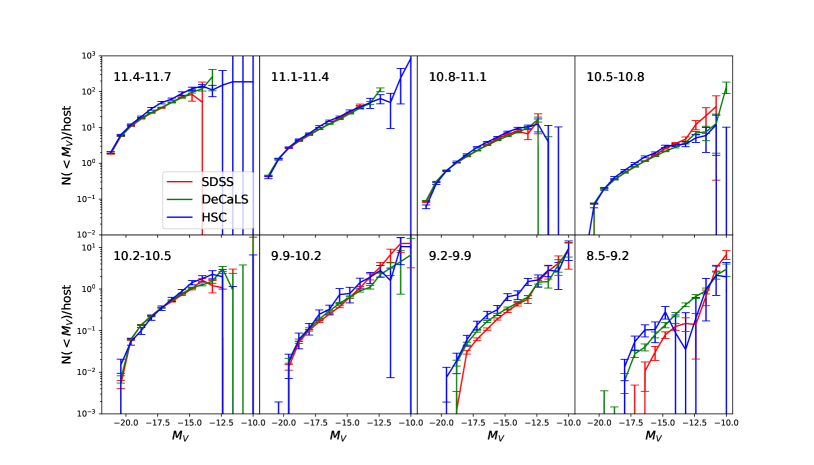
Figure 2: Cumulative $V$-band luminosity functions (LFs) for satellite galaxies projected within the halo virial radius to isolated central galaxies (ICG1s) in HSC, DECaLS and SDSS (see the legend). In addition, an inner radius cut of $r_{p}>30$ kpc has been adopted for all three surveys to avoid failures in source deblending. Flux limits are adopted to be $r<21$, $r<22.5$ and $r<25$ for SDSS, DECaLS and HSC, respectively. The text in each panel indicates the log stellar mass range of primaries. Errorbars are 1-$\sigma$ scatters based on 100 boot-strap subsamples.

As have been introduced in Section 2, HSC, DECaLS and SDSS have very different survey depth and resolution. The deeper a survey is, the more fainter sources and the more extended low surface brightness structures can be detected, and thus the observed field is more crowded. As a result, deep surveys such as HSC suffer from more serious source blending issues than other shallower surveys. Details about direct comparisons among the three surveys are provided in Appendix A. As the readers can see from Figure 13, there are far more faint sources detected in HSC and around the central primary galaxies. Some sources are real, which are failed to be detected in both SDSS and DECaLS. However, some sources are in fact fake detections, which are in the photometric region of the central galaxy itself and are mistakenly deblended to be companions.

To avoid such deblending failures on small scales to the central primaries, we adopt an inner radius cut of $r_{p}>30$ kpc for all the results in the main text of this paper. We also provide results in Appendix A showing the evidences supporting the choice of $r_{p}>30$ kpc. We also found that failures of source deblending is more frequent around blue primaries, because blue galaxies have rich substructures such as star-forming regions along the spiral arms, which are more easily to be mistakenly deblended as companion sources. Thus the inner radius cut is very important in order to properly avoid the deblending failures and ensure consistencies among HSC, DECaLS and SDSS.

The inner radius cut not only excludes fake sources, but real sources within $r_{p}\sim$30 kpc are also excluded. This, however, does not affect the fair comparison among different surveys if we adopt the same cut for all of them. In addition, to ensure fair comparison with the MW satellite LF, we need to properly consider the projection effect. This is because extra-galactic satellites are observed in projection, whereas the MW satellites are observed in 3-D. We choose to project the observed 3-D positions of MW satellites along 600 randomly selected “line-of-sight” directions. For each direction of projection, we calculate the satellite LF after excluding satellites projected within 30 kpc. In the end, we calculate the mean MW satellite LF based on all 600 projections, and the 1-$\sigma$ scatter among these different projections is adopted to represent the uncertainties. The inner radius cut of 30 kpc always excludes Sagittarius-I in Table LABEL:tbl:MWsat from our analysis, due to its short Galactocentric distance of $r_{\rm GC}=18.3\pm 2.0$ kpc. The other MW satellites we use for the comparison are at distances greater than 30 kpc, although the projection would make satellites appear to be closer than this distance cut in some cases.

In the end, we note that the MW satellite LF is measured in $V$-band. However, we do not have $V$-band data for any of the three surveys used in this study. To ensure fair comparisons, we convert the $r$-band magnitudes to $V$-band based on the transformations provided by Blanton & Roweis (2007) and by using the $g-r$ colours of satellites.

4 Results

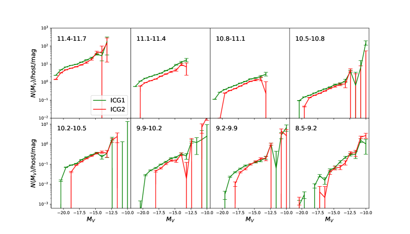
Figure 3: Differential $V$-band LFs for satellite galaxies projected between 30 kpc and the halo virial radius, and centred on two different populations of isolated central galaxies (ICG1 and ICG2). The results are based on DECaLS. Companions of ICG1s are required to be fainter than ICG1s, while companions of ICG2s are at least one magnitude fainter. Due to the selection, ICG2s have less satellites, which could be an indication of smaller host halo mass. Errorbars are 1-$\sigma$ scatters based on 100 boot-strap subsamples.

In this section we present our satellite LF measurements. First, we show results for all primary galaxies grouped into eight stellar mass bins, and we investigate whether the satellite LF depends on the magnitude gap between the central primary galaxy and its satellites, using ICG1s and ICG2s. Then we move on to present results focusing on isolated central galaxies (or galaxy pairs) sharing similar properties as our MW (or as the MW and M31), and compare the measurements with the MW satellite LF.

4.1 Satellites of all primary galaxies

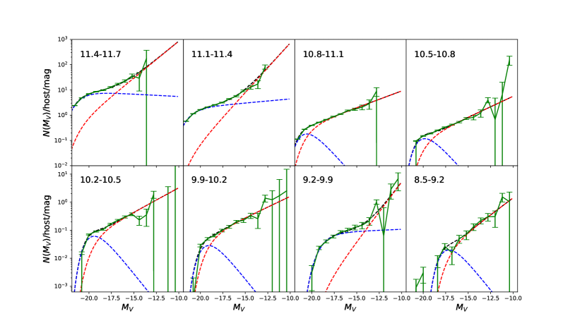
Figure 4: Differential $V$-band LFs for satellite galaxies projected between 30 kpc and the halo virial radius to ICG1s in DECaLS. Errorbars are 1-$\sigma$ scatters based on 100 boot-strap subsamples. Double Schecter functions are fit to the LFs. Black dashed curves show the best fits, while the two components are plotted as blue and red dashed curves.

Table 3: The best-fit double Schecter function parameters to satellite LFs around ICG1s in Figure 3.

$\log M_{\ast}/M_{\odot}$	$M_{0}$	$\Phi_{\ast,1}$	$\Phi_{\ast,2}$	$\alpha$	$\beta$
11.4-11.7	$-$21.27$\pm$0.10	9.662$\pm$0.567	0.477$\pm$0.703	$-$0.953$\pm$0.111	$-$1.730$\pm$0.251
11.1-11.4	$-$21.42$\pm$0.10	2.038$\pm$0.163	0.026$\pm$0.035	$-$1.081$\pm$0.064	$-$1.979$\pm$0.444
10.8-11.1	$-$20.56$\pm$0.05	0.532$\pm$0.045	0.393$\pm$0.017	$-$0.000$\pm$0.251	$-$1.332$\pm$0.018
10.5-10.8	$-$19.83$\pm$0.04	0.346$\pm$0.024	0.141$\pm$0.012	$-$0.000$\pm$0.028	$-$1.416$\pm$0.034
10.2-10.5	$-$19.42$\pm$0.06	0.180$\pm$0.021	0.080$\pm$0.010	$-$0.000$\pm$0.040	$-$1.437$\pm$0.047
9.9-10.2	$-$19.06$\pm$0.19	0.084$\pm$0.028	0.072$\pm$0.013	$-$0.000$\pm$0.287	$-$1.381$\pm$0.071
9.2-9.9	$-$18.81$\pm$0.29	0.088$\pm$0.026	0.001$\pm$0.002	$-$-1.035$\pm$0.121	$-$2.064$\pm$0.138
8.5-9.2	$-$17.15 $\pm$0.38	0.058$\pm$0.036	0.029$\pm$0.015	$-$0.000$\pm$0.144	$-$1.601$\pm$0.159

Figure 2 shows the LFs for satellite galaxies projected between 30 kpc and the halo virial radius to ICG1s in HSC, DECaLS and SDSS, and ICG1s are grouped into eight stellar mass bins (see the text in different panels). Throughout this paper, the errorbars for extra-galactic satellite LFs are based on the 1-$\sigma$ scatters of 100 boot-strap subsamples, which reflect the errors on the mean satellite population of different primaries. We are able to measure the satellite LFs around primaries as small as $8.5<\log M_{\ast}/M_{\odot}<9.2$. The satellite LFs based on HSC, DECaLS and SDSS are very similar to each other in all of the panels. Considering the very different observational mode, data reduction, depth and image resolution, the consistency among these surveys is very encouraging.

There are, however, still some very small and delicate differences. At the bright end, the difference might be partly due to the small number of bright galaxies and hence relatively large sample variance. At fainter magnitudes, the difference could be caused by many reasons. First of all, different flux limits are adopted for the three surveys. In fact, we have explicitly tested that after adopting the same flux limit of $r<21$ for all surveys, the results in in Figure 2 remain almost unchanged. We avoid repeatedly showing the figure with $r<21$, but the readers can still find part of the tests based on a stellar mass bin similar to our MW in Section 4.2.

Secondly, we can see HSC measurements tend to show slightly higher amplitudes than both SDSS and DECaLS in almost all of the panels. This is at least partly due to the deeper surface brightness depth of HSC, and thus more low surface brightness satellites can be detected. While the integrated flux of a faint satellite is still above the survey flux limit, it might not have been detected because it is diffuse and has low surface brightness (e.g. Danieli et al., 2018; Carlsten et al., 2020c). We provide more evidences in Appendix A.

In addition, given the different image resolution or PSF size, the ability for different survey pipelines to deblend sources can vary. HSC is able to disentangle multiple sources which have very small angular separations, whereas SDSS might treat them as one single source. This could cause some very delicate differences in both satellite number counting and magnitudes.

Moreover, the photometric system, data reduction steps and depth of different surveys are not the same, and the magnitudes are defined and calculated in different ways. As a result, even for the same source, its magnitudes in HSC, DECaLS and SDSS can differ. However, the filter system between SDSS and HSC is very similar, and as have been checked in Qiu et al. (2020), the mean magnitude difference between the same source in SDSS and HSC is negligible, and thus we do not expect the difference in magnitudes can significantly affect our results. We provide in Appendix A (Figure 16) more detailed comparisons by using matched sources between different surveys.

Lastly, we have excluded photometric sources with a few bad-quality photometric flags setting up to be true, including bad pixels, saturated, edge, cosmic rays and so on (see Section 2 for details). However, it is difficult to have exactly the same selection by photometric flags for different surveys. We have tested that after removing the selection by photometric flags, and the change in measured satellite LFs is smaller than 1%.

For primaries more massive than $\log M_{\ast}/M_{\odot}\sim 10.8$, we can robustly push down to $M_{V}\sim-14$ or $-13$. Results based on HSC can push even fainter (close to $M_{V}\sim-10$ in the two most massive bins), but the measurements are quite noisy due to the small HSC footprint. For smaller primaries, we can push close to $M_{V}\sim-10$. This is because massive bright primaries are biased to have higher redshifts, but for fainter luminosity bins, only those satellites around more nearby primaries are complete and are allowed to contribute to the satellite counts (see Section 3 for details). Thus we do not have enough number of nearby massive bright primaries contributing to the number counts of intrinsically faint satellites. On the contrary, smaller and fainter primaries have lower redshift distributions, and thus we are able to push down to even fainter magnitudes for satellites around them.

Previous measurements of satellite LFs based on SDSS can go as faint as $M_{r}\sim-14$ (e.g. Wang & White, 2012) or about $M_{V}\sim-14$ as well (e.g. Guo et al., 2011b), i.e., at most $\sim$8 magnitudes fainter than the central primaries. Very recently, after carefully considering the varying survey depths, new measurements of satellite LFs based on DECaLS can also reach $M_{r}\sim-14$ (Tinker et al., 2019). Note the measured satellite LFs in Wang & White (2012) stopped at the stellar mass of $\log_{10}M_{\ast}/M_{\odot}=10.2$ for primaries. In this study, we have managed to extend the previous measurements down to much fainter satellites ($M_{V}\sim-10$) and around smaller primaries ($9.9<\log_{10}M_{\ast}/M_{\odot}<10.2$, $9.2<\log_{10}M_{\ast}/M_{\odot}<9.9$ and $8.5<\log_{10}M_{\ast}/M_{\odot}<9.2$).

The stellar mass of the LMC is likely to be in between the two lowest stellar mass bins in our analysis. The LMC should have its own satellites before merging into our Galaxy. Many efforts have been devoted to potentially determine how many satellites does the LMC have before infall (e.g. Deason et al., 2015; Jethwa et al., 2016; Sales et al., 2017; Shao et al., 2018a), which still tend to show large uncertainties. As have been pointed out by Dooley et al. (2017), it is useful to look at the population of satellites around isolated galaxies with LMC stellar mass, and these isolated LMC-like systems are also important for the study of environmental effects on the evolution of dwarf galaxies (e.g. Wetzel et al., 2015). Our measurements predict an average number of 3–8 satellites brighter than $M_{V}\sim-10$ of LMC-mass ICGs.

Unfortunately, despite the much deeper survey depths of $r<25$, HSC does not seem to be able to push significantly fainter than DECaLS ($r<22.5$) or SDSS ($r<21$). This is mainly due to the much smaller footprint of HSC (a bit more than 450 square degrees) than the other two surveys. The footprints of SDSS and DECaLS are above 8,000 and 9,000 square degrees, respectively. However, it is still very encouraging that even given the more than ten times smaller footprint, HSC is still able to achieve comparable or slightly better performance. Hence it is promising to wait for the completion of the HSC mission and use the full 1,400 square degrees of the planned footprint to push even fainter. Besides, our results based on HSC can be regarded as a pioneer study of the future LSST survey, which is designed to have similar depth but much larger footprint (about 23,000 sq. deg.) than HSC. Our results based on HSC have demonstrated the power of such deep surveys to help revolutionise our understanding towards faint extra-galactic satellites.

Compared with ICG1s, ICG2s are selected with more strict criteria, i.e., its companions should be at least one magnitude fainter. Now we move on to compare satellite LFs measured around ICG1s and ICG2s. The results are shown in Figure 3. We only show the differential LFs based on DECaLS, because of its larger footprint than HSC and greater depth than SDSS, though we have explicitly checked that HSC and SDSS show very similar results. Green curves are based on ICG1s, while red curves are based on ICG2s, and due to the larger magnitude gap between the primaries and their companions, the bright end cut off of satellite LFs around ICG2s becomes more significant by definition. In addition, we also see that the LFs around ICG2s tend to have lower amplitudes than those around ICG1s, and this is true over the wide luminosity range probed here.

The difference between ICG1s and ICG2s is very interesting. Although we have only changed the magnitude gap between primaries and their companions in our selection, the magnitude gap affects not only the bright end, but also the overall abundance of satellite galaxies at different magnitudes. Many previous studies have tried to link satellite abundance or total satellite luminosity to host halo mass (e.g. Wang & White, 2012; Sales et al., 2013; Wang et al., 2014; Tinker et al., 2019), and such links have been proved by Mandelbaum et al. (2016) through direct weak lensing measurements. Thus the lower amplitudes for ICG2s in Figure 3 imply that ICG2s are likely hosted by less massive haloes. This is also supported by studies based on numerical simulations, which claim that the host halo mass depends on the magnitude gap between central and satellite galaxies (e.g. Lu et al., 2015). About the nature of why such magnitude gaps can be linked to satellite abundance or halo mass, it might be related to the assembly history of haloes, which we will investigate in future studies.

We fit the following double Schecter functions to satellite LFs in DECaLS (green curves in Figure 2 and 3)

$$\Phi(L)\mathrm{d}L=\left\{\Phi_{\ast,1}\left[\frac{L}{L_{0}}\right]^{\alpha}+\Phi_{\ast,2}\left[\frac{L}{L_{0}}\right]^{\beta}\right\}\exp{\left(-\frac{L}{L_{0}}\right)}\mathrm{d}L,$$ (2)

and because the relation between luminosity and absolute magnitude is $\frac{L}{L_{0}}=10^{-0.4(M-M_{0})}$, Equation 2 can be expressed in terms of absolute magnitude $M$ as

$$\Phi(M)\mathrm{d}M =0.4\ln{10}$$

$$\times\left[\Phi_{\ast,1}10^{-0.4(M-M_{0})(\alpha+1)}+\Phi_{\ast,2}10^{-0.4(M-M_{0})(\beta+1)}\right]$$

$$\times\exp{\left[-10^{-0.4(M-M_{0})}\right]}\mathrm{d}M.$$ (3)

The best fits are shown in Figure 4, in which we present the differential satellite LFs instead of cumulative ones. The best-fit parameters are provided in Table LABEL:tbl:LFpara. Except for the stellar mass bin of $9.2<\log_{10}M_{\ast}/M_{\odot}<9.9$, which has a faint end slope slightly steeper than $-2$, the best-fit faint end slopes of all the other panels are shallower than $-2$. In addition, there are some indications in the top right panel that the faint end tends to show some signs of up-turning. The measurements at the faint end are quite noisy, and thus we avoid drawing a very strong conclusion in this paper. However, the faint end slopes of satellite LFs have very important cosmological implications. For example, the predicted number of substructures by warm and cold dark matter models only vary at the small mass end (e.g. Lovell et al., 2014), and if the satellite LF continues to rise sharply at the faint end, the rich number of small satellites can provide important clues to distinguish different dark matter models. In addition, the faint end slopes of satellite LFs contain information about the formation history of galaxies at the early Universe and can be used to constrain models of galaxy formation (e.g., Lim et al., 2017; Lan et al., 2016). Future deep and wide photometric surveys such as LSST, combined with our method of counting photometric satellites around spectroscopic primaries, is thus very promising and powerful to help improving the statistics at the faint end and hence can potentially revolutionise our understanding towards the nature of extremely faint and small satellites, though one has to very carefully deal with possible systematics at such faint magnitudes.

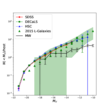
Figure 5: Cumulative $V$-band LFs for satellite galaxies projected between 30 and 260 kpc to MW-mass ICG1s ($10.63<\log_{10}M_{\ast}/M_{\odot}<10.93$). Results based on SDSS, DECaLS and HSC are overplotted with each other for comparisons (see the legend). Flux limits are adopted to be $r<21$, $r<22.5$ and $r<25$ for SDSS, DECaLS and HSC, respectively. Black solid histogram shows the cumulative LF for MW satellites after projection and with the same inner radius cut of $r_{p}>30$ kpc. Errorbars for HSC, DECaLS and SDSS results are 1-$\sigma$ scatters based on 100 boot-strap subsamples, which reflect the error on the averaged satellite LF. Errorbars for the MW satellite LF are calculated from the 1-$\sigma$ scatters among 600 different projections. Green triangles show predictions by the 2015 L-Galaxies model, and the green shaded region associated with it shows the scatter, i.e. 16th 84th percentiles, in the LFs of individual systems.

4.2 Satellites of Milky-Way-like primary galaxies

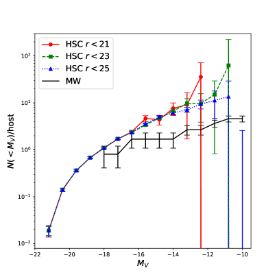
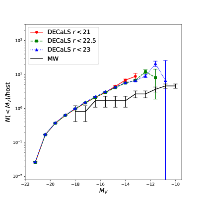
Figure 6: Left: Cumulative $V$-band LFs for satellite galaxies projected between 30 and 260 kpc to MW-mass ICG1s ($10.63<\log_{10}M_{\ast}/M_{\odot}<10.93$). The results are based on HSC. Three different flux limits of $r<21$, $r<23$ and $r<25$ are adopted. LFs based on different flux limits show very good agreement with each other, which validates our method and the sample completeness of HSC. Right: Similar to the left panel, but shows results based on DECaLS. Three different flux limits of $r<21$, $r<22.5$ and $r<23$ are adopted. In both panels, the black solid histogram shows the cumulative LF for MW satellites after projection and with the same inner radius cut of $r_{p}>30$ kpc. Errorbars are calculated in the same way as Figure 5.

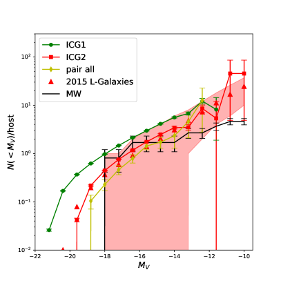
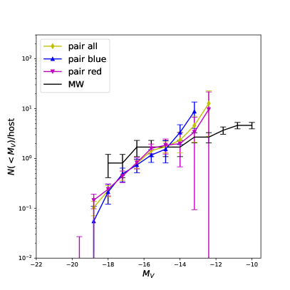
Figure 7: Left: Cumulative $V$-band LFs for satellite galaxies projected between 30 and 260 kpc to ICG1s, ICG2s and primary galaxies in pair (see the legend). All different types of primary galaxies are required to have similar stellar mass as our MW, i.e., $10.63<\log_{10}M_{\ast}/M_{\odot}<10.93$. In addition, although upon selecting galaxy pairs, the mass ratio between the two galaxies in pair is required to be smaller than a factor of two, the stellar mass of the companion is not necessarily in the range of $10.63<\log_{10}M_{\ast}/M_{\odot}<10.93$. For such cases, only one galaxy in the pair is used for this plot, while the other is not. This maximises our sample size. Red triangles show the predicted satellite LFs of ICG2s by the 2015 L-Galaxies model, and the red shaded region associated with it shows the scatter, i.e. 16th 84th percentiles in the LFs of individual systems. Right: Similar to the left plot, but shows the satellite LFs of all, red and blue primary galaxies in pair (see the legend). The yellow curve is exactly the same in both plots. For red or blue central galaxies in pair, no restrictions are made to the colour of the other companion. Results in both plots are are based on DECaLS. The black solid histogram shows the cumulative LF for MW satellites after projection and with the same inner radius cut of $r_{p}>30$ kpc. Errorbars are calculated in the same way as Figure 5.

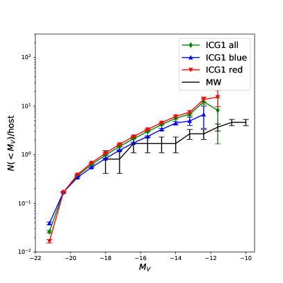
Figure 8: Cumulative $V$-band LFs for satellite galaxies projected between 30 and 260 kpc to all, red and blue ICG1s with stellar mass in the range of $10.63<\log_{10}M_{\ast}/M_{\odot}<10.93$. Errorbars are calculated in the same way as Figure 5.

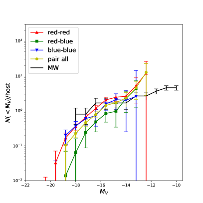
Figure 9: Cumulative $V$-band LFs for satellite galaxies projected between 30 and 260 kpc to primary galaxies in pair. A few different colour combinations are adopted for the two primary galaxies, i.e., “red-red”, “blue-blue” and “red-blue”. “pair all” is exactly the same as the yellow curve in Figure 7. Primaries are required to have similar stellar mass to our MW, i.e., $10.63<\log_{10}M_{\ast}/M_{\odot}<10.93$, but the stellar mass of the other companion is not necessarily in this range and hence might not be used for this plot. All results are based on DECaLS. The black solid histogram shows the cumulative LF for MW satellite galaxies after projection and with the same inner radius cut of $r_{p}>30$ kpc. Errorbars are calculated in the same way as Figure 5.

According to the recent study by Licquia & Newman (2015), the total stellar mass of our MW is about $(6.08\pm 1.14)\times 10^{10}M_{\odot}$. Centred on this value, Figure 5 shows satellite LFs around ICG1s in the stellar mass range of $10.63<\log_{10}M_{\ast}/M_{\odot}<10.93$. Results based on HSC, DECaLS and SDSS show very good agreement with each other, though HSC tends to show slightly higher amplitudes, and as have been discussed in the previous section, this is likely real (more details can be found in Appendix A).

All results tend to have higher amplitudes and steeper slopes than the MW satellite LF, and the tension with the MW satellite LF is much more significant than the errorbars. The errors of the MW satellite LF are based on the 1-$\sigma$ scatters of 600 random projections, and thus the errors are smaller at the faint end, where the cumulative number of satellites becomes larger and less sensitive to the projected inner radius cut. Besides, it is very important to remember that the boot-strap errors cannot be used to quantify the intrinsic scatter.

With our statistical satellite counting and background subtraction methodology, it is difficult to directly infer the scatter, but we can estimate the scatter through the satellite LFs from numerical simulations. To select ICG1s in simulations, we project the simulation box along the $z$ direction, and assign each galaxy a “redshift” based on its coordinate and velocity along the projected direction. ICG1s can then be selected using the same isolation criteria as for real data. For each ICG1, its satellites are counted within a 3-dimensional sphere with radius of 260 kpc. Besides, we apply an inner radius cut of $r_{p}>30$ kpc perpendicular to the $z$ direction.

The green triangles and the shaded region in Figure 5 show the averaged satellite LF and the scatter for ICG1s selected from the 2015 L-Galaxies mock galaxy catalogue. At the bright end, the numbers of satellites around most primaries are either zero or one, and thus the scatter is not shown. The green triangles are slightly lower in amplitudes than the results based on real data, which is partly due to the difference between satellite counts made in projection and in 3-dimensional coordinates, but the overall agreement at fainter magnitudes is very good. The scatter, however, is very large. Despite the fact that the discrepancy between the MW satellite LF and our measurements of extra-galactic satellite LFs is significantly larger than the boot-strap errorbars, the discrepancy is much smaller than the scatter at $M_{V}<-14$, and is still marginally consistent with the scatter at $M_{V}\sim-13$.

Figure 6 shows results based on HSC (left) and DECaLS (right), and we have tried a few different flux limits for each survey. Despite the difference in flux limits, the agreement is extremely good, indicating our satellite counting methodology works very well. The good agreement also proves the completeness of both surveys. However, we note that at $M_{V}>-15$, results based on fainter flux cuts tend to have slightly lower amplitudes than those with brighter cuts, though the differences are mostly smaller than the errors. This might indicate some small amount of incompleteness, due to, for example, failures in detecting low surface brightness satellites or mis-classifications of galaxies as stars. These small differences at the faint end, however, cannot violate the conclusions of this paper.

Now we start to compare MW satellites with the satellites around central primary galaxies selected in different ways. We will only show results based on DECaLS. This is because its footprint is larger than HSC and thus can include more galaxy pairs. Besides, the flux limit is deeper than SDSS, and thus the signal is better at faint ends. As we have explicitly checked, results based on HSC and SDSS are consistent. The left plot of Figure 7 shows the satellite LFs measured around ICG1s, ICG2s and primary galaxies in pairs. The green curve (ICG1s) is exactly the same as the one in Figure 5. As we have already investigated in Figure 3, the amplitude of satellite LFs around ICG2s is lower. The bright end cutoff also becomes more significant. As a result, the agreement with the MW satellite LF at the bright end is better, while the tension at fainter luminosities is smaller but still remains.

Similar to Figure 5, the prediction by the 2015 L-Galaxies model for satellite LF of ICG2s agrees very well with the real data. At $M_{V}<-12$, the discrepancy between the MW satellite LF and the L-Galaxies model prediction is within the scatter. This is consistent with previous studies (e.g. Guo et al., 2015a; Shao et al., 2018a), which also show that the mean/median satellite LFs predicted by simulations tend to have higher amplitudes than the MW satellite LF, while they still agree within the scatter. However, at the faint end ($M_{V}>-12$), our measurements show that the difference between the averaged extra-galactic and the MW satellite LFs is larger than the scatter. In fact this is also revealed in Figure 2 of Guo et al. (2015a) and Figure 1 of Shao et al. (2018a), that the MW satellite LF is below those for most of the MW-mass systems in the simulation at $M_{V}>-12$. We will come back discussing the tension between extra-galactic and the MW satellite LF in Section 5.3.

The yellow curve in Figure 7 shows the result for primary galaxies in pairs similar to the MW and M31. The LF shows stronger bright end cutoff. Compared with the MW satellite LF, the yellow curve has slightly lower amplitudes at the bright end, and higher amplitudes at $M_{V}>-15$. In fact, for primaries selected in these different ways, their averaged satellite LFs all tend to have steeper slopes and higher amplitudes at $M_{V}>-15$ than the MW satellite LF.

It has been shown in previous studies that red isolated primaries have more satellites and are hosted by more massive dark matter haloes than blue primaries with the same stellar mass (e.g. Wang & White, 2012; Wang et al., 2014; Mandelbaum et al., 2016; Man et al., 2019), and thus we further split our sample of primaries in pairs into red and blue populations. As has been mentioned in Section 2, this is achieved by a stellar mass dependent division of ${}^{0.1}(g-r)=0.065\log_{10}M_{\ast}/M_{\odot}+0.1$ over the colour-magnitude diagram of SDSS spectroscopic galaxies. The readers can find more details in Wang & White (2012). The satellite LFs of red and blue primaries in pair are shown as magenta and cyan curves in the right plot of Figure 7. There is no significant difference between the satellite LFs around red or blue primary galaxies in pair, and the tension with the MW satellite LF is still present. Note that when cumulating satellite counts around one of the primary galaxies in the pair, we did not include any additional requirements on the colour of the other primary.

As a comparison, we also show in Figure 8 the satellite LFs around all, red and blue ICG1s. The number of red and blue MW-mass ICG1s (46352 and 33488) is significantly larger than the number of red and blue primary galaxies in pair (893 and 738). Thus the errorbars are much smaller. Red ICG1s in Figure 8 tend to have more satellites, which is consistent with conclusions in previous studies.

While the small sample size and large errorbars probably have prevented us from tracking any significant differences between red and blue primaries in pair, we now move on to investigate satellite LFs for galaxy pairs with different colour combinations. This is shown in Figure 9 for red-red (red curve), blue-blue (blue curve) and red-blue (green curve) pairs. We also overplot the yellow curve for all primary galaxies in pair from Figure 7. The numbers of galaxies in red-red, blue-blue and red-blue pairs are 524, 341 and 766, respectively. There are two interesting features. First of all, different colour curves all have steeper slopes than that of the MW satellite LF, and are lower in amplitudes at the bright end and higher in amplitudes beyond $M_{V}\sim-15$ than the MW satellite LF. Moreover, despite the large errorbars and the failure of tracking down any significant difference in the previous Figure 7, now we can clearly see that red-red and blue-blue pairs both have more satellites than red-blue pairs (see Section 5.2 for more details about the significance).

Under the standard framework of cosmic structure formation, red galaxies formed early and grew fast at early stages, which then triggered feedback prohibiting late-time star formation activities, while their host dark matter halo and satellite populations keep growing through accretion. As a result, at fixed halo mass, the stellar mass of red galaxies tends to be smaller than that of blue galaxies, because red galaxies have stopped forming stars.

Therefore, red galaxies having more satellites can be explained under the standard cosmological model, and as have been checked by Wang & White (2012) (also see, e.g., Wang et al., 2014; Man et al., 2019), the trend can be reproduced by modern galaxy formation models. It is thus straight-forward to understand why red-red galaxy pairs can have more satellites than primaries in pair with other colour combinations. However, it is still puzzling why galaxies in blue-blue pairs tend to have more satellites than red-blue pairs in Figure 9, given the fact that blue isolated galaxies do not show such a trend. In Section 5, we provide more discussions, including a comparison with the prediction by Illustris TNG-100.

5 Discussions

5.1 Comparison with Illustris TNG-100

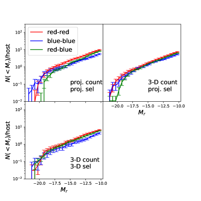
Figure 10: Cumulative $r$-band LFs for satellite galaxies around MW-mass primary galaxies in pair from Illustris TNG-100. Top Left: Primaries are selected in projection, and satellite counts are made in projection (30 kpc $<r_{p}<$ 260 kpc), with statistical fore/background subtractions. Top Right: Primaries are selected in projection, and satellite counts are made in 3-D (30 kpc $<r<$ 260 kpc). Bottom Left: Primaries are selected in 3-D, and satellite counts are made in 3-D as well. Errorbars are the 1-$\sigma$ scatters of 100 boot-strap subsamples.

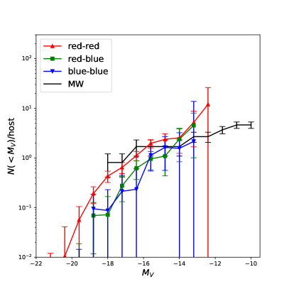
Figure 11: Cumulative $V$-band LFs for satellite galaxies projected between 30 and 260 kpc to MW-mass primary galaxies in pair. Galaxy pairs are selected in the same way as those in previous figures, but the flux limit is chosen as $r<16.7$. Black solid histogram shows the cumulative LF for detected MW satellite galaxies after projection and with the same inner radius cut of $r_{p}>30$ kpc. Errorbars are calculated in the same way as Figure 5.

We have shown that the averaged satellite LF of blue-blue primary galaxies in pair have higher amplitudes than that of primaries in pair with red-blue colour combinations. Here we start our investigation by checking whether modern numerical simulations can reproduce such a trend. We use the publically released Illustris TNG-100 halo and subhalo catalogues for the analysis. We choose to use TNG-100 instead of the L-Galaxies model for our purpose here, because the colour distribution predicted by TNG-100 is in better agreement with real data, and there are not enough blue-blue MW-mass galaxy pairs in the 2015 L-Galaxies model.

To select primary galaxies in pair and in analogy to those in SDSS/DR7, we project the simulation box along $x$, $y$ and $z$-directions, and each galaxy can be assigned a “redshift” based on its coordinate and velocity along the projected direction. Galaxy pairs are then selected with exactly the same isolation criteria as those introduced in Section 2. Besides, we also select galaxy pairs in 3-dimensional coordinates, by applying the selection along the direction perpendicular to the line of sight to the 3-dimensional distance separations of galaxies in the simulation. We denote the two selections by “proj. sel” and “3-D sel”.

Satellites counts are made in projection or in 3-dimensional coordinates. The counts made in projection is analogous to real observation. For each projection, we first count companions projected within a cylinder, including those fore/background galaxies. The fore/background counts are then subtracted statistically through the counts around random points. The counts of all primaries and in all three projected directions ($x$, $y$ and $z$) are cumulated and averaged in the end. On the other hand, when counting satellites in 3-dimensional coordinates, we simply draw a sphere centred on each primary and count companions within the sphere. Satellites counted in the two different ways are denoted as “proj. count” and “3-D count”.

The satellite LFs are calculated directly from the absolute magnitudes of galaxies in TNG-100. We did not construct and use light-cone mock catalogues, and thus the direct projection of simulation box cannot fully represent the depth in background counts of a given flux limit. However, as we have very carefully checked and explicitly shown in the Appendix of Wang & White (2012), results based on directly projecting the simulation box and based on full light-cone mock catalogues are very similar to each other, though the latter is nosier due to its much larger background level.

Figure 10 shows the satellite LFs of primary galaxies in pair from TNG-100. Similar to Figure 9, we try different colour combinations for the galaxy pair. The methods of primary selection and satellite counting are indicated by the text in each panel. Note that due to the resolution limit of TNG-100, the satellite LFs beyond $M_{V}\sim-16$ tend to be flattened, but we think this will not affect our comparison unless the satellite distributions around red and blue primaries are affected differently.

In all three panels of Figure 10, satellite LFs around blue-blue galaxy pairs do not show higher amplitudes than other colour combinations at $M_{r}>-17.5$. At the bright end, the blue curves tend to show higher or comparable amplitudes as the green curve, which is more similar to what we see in real data. Except for the bright end, TNG-100 does not reproduce similar trends as the real observation.

When the selection is made in projection, the number of primary galaxies in red-red, blue-blue and red-blue pairs are about 61, 46 and 91 (for $x$, $y$ and $z$ directions added together), out of which 53, 44 and 89 are true halo central galaxies, respectively. The numbers are small, but is already enough for us to check the trend, and at least in the simulation, the purity of galaxy pairs is high, and our results seem unlikely to have been affected by contamination of satellites in our sample of primary galaxies.

5.2 Why are there more satellites around blue-blue primary galaxy pairs?

We estimate the significance of the difference between satellite LFs around blue-blue and red-blue galaxy pairs by assuming a $\chi^{2}$ distribution

$$\chi^{2}=\sum_{i,j}D_{i}\times[C^{-1}]_{ij}\times D_{j},$$ (4)

where $D_{i}$ means the difference between the $i$-th data point of the blue and green curves in Figure 9. $C^{-1}$ is the inverse of the covariance matrix, and is contributed by the covariance of both measurements, i.e., $C=C_{\mathrm{blue-blue}}+C_{\mathrm{red-blue}}$. The estimated significance is 2.70-$\sigma$. If the detection is genuine and robust, some new physical mechanisms beyond the merging origin of satellites under the standard cosmological context have to be proposed, for example, tidal dwarf galaxies.

It has been discovered and reported as the 1-halo “Galactic Conformity” phenomenon that blue galaxies also tend to have bluer satellites with stronger star formation and more cold gas supplies, mainly because they are hosted by less massive dark matter haloes than red galaxies with the same stellar mass(e.g. Weinmann et al., 2006; Yang et al., 2006; Kauffmann et al., 2010; Wang & White, 2012). The richer cold gas supplies seem to support the formation of tidal dwarf galaxies. However, it is hard to explain why in Figure 7, if we do not include any restriction on the colour of the other primary galaxy in the pair, blue primaries do not have more satellites. It is thus still puzzling why there are more satellites around blue-blue galaxy pairs than red-blue galaxy pairs in real data. The mechanism might be related to the large scale environment, based on the fact that we only see such signals when both galaxies in the pair are blue.

We have also checked the robustness of our results by repeating the calculation using galaxy pairs selected with different criteria. In the previous figures, galaxy pairs are selected by requiring that, centred on the middle point of the pair, all other companions projected within 800 kpc and within seven times virial velocity of the more massive galaxy in the pair and along the line of sight should be at least one magnitude fainter. We have tried to vary the projected separation to 1,500 kpc and the magnitude gap to 0.5. With the new selection, the sample size is decreased by about 1/3, and the measurements still show that there are more satellites around blue-blue galaxy pairs than red-blue pairs, but the significance drops to 1.79-$\sigma$.

However, when we fix the selection to be the same as that of Figure 9, but change the flux limit from $r<17.7$ to $r<16.7$, we fail to see significant difference between the amplitudes of blue and green curves. This is shown in Figure 11. Thus the detection does not seem to be robust against the variation in the flux limit or redshift range of primaries, as a brighter flux limit leads to a lower redshift range. This indicates our results are likely affected by large cosmic variations for the small number of galaxy pairs at low redshifts. Therefore, we avoid drawing a strong conclusion that blue-blue galaxy pairs have more satellites than red-blue pairs. Our results await more detailed follow-up studies by looking at, for example, galaxies pairs, their satellites and the evolution at higher redshifts.

5.3 Is our MW special?

As have been introduced, a few so-called challenges to the standard cosmological model were claimed, based on the observed properties of satellite galaxies in our MW (e.g. Klypin et al., 1999; Moore et al., 1999; Boylan-Kolchin et al., 2011b). However, conclusions relying on the population of satellites in a single host galaxy might be unfair, as we don’t know whether our MW is typical among galaxies of its type. This is why we looked at extra-galactic satellite systems in this study. Our investigations show that the averaged satellite LFs around MW-mass central primary galaxies selected in different ways tend to have more similar amplitudes to the MW satellite LF at the bright end, but the slopes at fainter magnitudes are significantly steeper, and the amplitudes beyond $M_{V}\sim-15$ are higher.

Explicitly, at the bright end, ICG1s and ICG2s on average tend to have comparable number of satellites as our MW, while primary galaxies in pair tend to have a bit stronger bright end cutoff and lower amplitudes at $M_{V}<-16$ than the MW satellite LF. The average number of satellites with $M_{V}<-16$ are about 1.5 and 2.5 around ICG1s and ICG2s. This is consistent with our MW, which has the LMC and SMC. It seems our results at the bright end are not quite consistent with the estimates by Liu et al. (2011), in which the probability for isolated galaxies with luminosities similar to our MW and having two satellites about $\Delta M_{V}=2$ and $=4$ magnitudes fainter is reported to be only 3.5%.

Liu et al. (2011), however, adopted slightly more strict isolation criteria to select central primaries, and they counted satellites within a projected distance of 150 kpc. Their sample of MW-like primaries are selected according to luminosity. To ensure a fair comparison, we repeat our analysis by adopting the same selection of primaries as Liu et al. (2011), and we use primaries with $-21.05<M_{V}<-20.75$ (or $M_{{}^{0.1}r}\sim-21.2$) and the same projected separation of 150 kpc to count satellites. Compared with ICG1s, the amplitude indeed drops, but the cumulative LF is still comparable to that of ICG2s at $-17<M_{V}<-15$, i.e., there are on average $\sim$1.5 such bright satellites with $M_{V}<-16$.

The fraction of dark matter haloes smaller than $M_{200}\sim 1.25\times 10^{12}M_{\odot}$ and hosting both LMC and SMC-like satellites is also reported to be very low by Boylan-Kolchin et al. (2011a), while the probability for more massive dark matter haloes hosting LMC and SMC-like satellites is significantly increased. According to recent studies, the virial mass of our MW is about $M_{200}\sim 1\times 10^{12}M_{\odot}$ (e.g. Callingham et al., 2019; Li et al., 2020), and the readers can check Wang et al. (2020) for a review. Thus although the predicted probability of hosting both LMC and SMC-like satellites by numerical simulations is rare, it actually happens with our MW, unless the best-fit virial mass of our MW is under-estimated. On the other hand, the fact that we found 1.5–2.5 satellites with $M_{V}<-16$ perhaps indicate that the mean host halo mass for other MW-mass central primaries is larger than that of our MW. This likely implies that our MW deviates from the mean stellar mass versus halo mass relation of other galaxies, which have been pointed out in previous studies (e.g. Guo et al., 2015a; Cautun et al., 2020).

Guo et al. (2011b) and Jiang et al. (2012) both reported a factor of two less extra-galactic satellites than the average of MW and M31 satellites with $M_{V}<-15$, which seem to be inconsistent with our results. This is, however, mainly because the satellite LF averaged over MW and M31 (Koposov et al., 2008) is boosted by the number of M31 satellites. M31 has 6 satellites with $M_{V}<-15$, while our MW only has two. This reflects the large diversity in the satellite LFs of different galaxies, and in the next subsection we will present the averaged satellite LF of more MW-mass systems in the Local Volume. Also note both Guo et al. (2011b) and Jiang et al. (2012) detected $\sim$2 satellites with $M_{V}<-15$ of MW-luminosity primaries on average, consistent with our results. Given our careful analysis in this paper and the consistency and cross checks with Guo et al. (2011b) and Jiang et al. (2012), we think our results are robust.

The other four satellites contributing to the MW satellite LF between $M_{V}\sim-14$ and $M_{V}\sim-10$ are Fornax, Leo I, Sculptor and Sagittarius I, among which Sagittarius I is always excluded due to the 30 kpc inner radius cut. The MW satellite LF contributed by these objects has a much shallower slope than those extra-galactic satellite systems, which leads to significantly lower amplitudes at $-15<M_{V}<-12$. Though faint satellite candidates of the MW are continuously being discovered (e.g. Homma et al., 2018, 2019), and future surveys, such as LSST, are predicted to increase the number of faint MW satellites by a factor of two to ten, depending on model assumptions (Newton et al., 2018; Simon, 2019), the number of such bright MW satellites with $M_{V}<-10$ is very unlikely to be significantly increased to match our measurements. Note the numbers of satellites around ICG1s and ICG2s with $M_{V}<-13$ are about ten and five, respectively. In addition, the extrapolated number of satellites with $M_{V}<-10$ around ICGs through the best-fit double Schecter function is about 33. Even if there is one more such bright satellite which sits behind the disc and is not yet discovered, the significance level can drop, but the discrepancy at the faint end cannot vanish.

The readers may wonder whether our satellite counts made in projection with statistical background subtraction may have been over-estimated, compared with the counts made in 3-dimensional coordinates. This is true because along the line-of-sight direction, the correlation between halo central galaxies and distant companions can persist out to very large distances, and companions with line-of-sight separations larger than the halo virial radius can still contribute to the signal. This explains why in Figure 10, the satellite LFs in the top left panel show slightly higher amplitudes than those in the top right panel. However, as have been carefully investigated in the Appendix of Wang & White (2012), by comparing results based on 3-dimensional coordinates and a full light-cone mock catalogue of galaxies, satellite counts made in projection are $\sim$30% more than those made in 3-dimensional coordinates for MW-mass primaries, and the fraction is almost independent of the luminosity of satellites. This is thus far from enough to explain the difference between the averaged extra-galactic satellite LFs and the MW satellite LF we see in this study.

Table 4: The probabilities quantifying how common is the MW satellite LF compared with the satellite LFs of ICGs, based on the assumption of the Poisson distribution ($P_{\mathrm{Poisson}}$) or on the predictions by the 2015 L-Galaxies model ($P_{\mathrm{sim}}$).

central primary	$P_{\mathrm{Poisson}}$ (30% decrease)	$P_{\mathrm{sim}}$
ICG1	$<$0.1%	1.2%
ICG2	$<$0.1%	1.5%

While the averaged extra-galactic satellite LFs show significant tensions with MW satellites, it is important to quantify how common is our MW compared with other MW-mass systems by accounting for the intrinsic scatter. We cannot directly calculate the satellite LF for each individual primary galaxy with our method. Instead, we choose to estimate the percentile fractions of extra-galactic satellite systems which are more atypical than our MW with two alternative approaches: i) assuming the underlying distribution of individual systems is Poissonian; ii) investigating the underlying scatter in satellite LFs using numerical simulations.

In the first approach, we assume that the averaged extra-galactic satellite LFs are representative of the underlying true LF, and that the MW satellite system is a random draw from the parent distribution, which is Poissonian. We can estimate the probability in each luminosity bin assuming the Poisson distribution as

$$P(k)=\frac{\lambda^{k}\exp{(-\lambda})}{k!},$$ (5)

where $\lambda$ is the average number of extra-galactic satellites in a given luminosity bin, and $k$ is the number of MW satellites in the same bin. $k$ is required to be integers. The number of MW satellites might not be integers after accounting for the projection effect by averaging over 600 random directions for projection, and thus we calculate the probability for each direction at first and take the median probability in the end. The MW satellite counts are either zero or one in each differential luminosity bin. If assuming the satellite counts in different luminosity bins are independent from each other, i.e., ignoring the error correlation, we can estimate the joint probability of MW satellites under the assumption of Poisson distribution as

$$P_{\mathrm{total}}=\prod_{i}P.CDF(k_{i}),$$ (6)

where $k_{i}$ refers to the satellite counts in the $i$-th luminosity bin, which are either zero or one, and $CDF$ means the cumulative probability function value of $P(k)$ up to $k_{i}$.

We then generate $10^{5}$ realisations by drawing from the random Poisson distribution of each magnitude bin, again assuming the averaged extra-galactic satellite LFs are the truth. The fractions of realisations that have a smaller probability than $P_{\mathrm{total}}$ are provided in Table LABEL:tbl:significance for ICG1s and ICG2s, which we denote as $P_{\mathrm{Poisson}}$. $P_{\mathrm{Poisson}}$ are much smaller than 0.1%. In this analysis, we have extrapolated the differential satellite LFs of ICG1s and ICG2s down to $M_{V}=-10.4$, based on the best-fit double Schecter functions. Note the data points in the three faintest bins are not used for the extrapolation because they are noisy, and the best-fit values are used instead to estimate $P_{\mathrm{Poisson}}$. We have also manually decreased the amplitude of the satellite LFs for ICG1s and ICG2s by 30%, to account for the difference between the global background subtraction and local or annular background subtractions (the over-estimates of satellite counts due to the correlated signal out to large distances, as discussed above).

$P_{\mathrm{Poisson}}$ depends on the extrapolations to the faint end, and as have been pointed out in previous studies, even at fixed halo mass, the true intrinsic scatter in satellite LFs can be larger than Poisson errors (e.g. Boylan-Kolchin et al., 2010; Cautun et al., 2014b). Thus in the second approach, we try to estimate the scatter and percentile fraction based on the satellite LFs from the 2015 L-Galaxies model. We choose to use L-Galaxies instead of TNG-100, because TNG-100 does not have enough resolution beyond $M_{V}\sim-16$.

The predicted satellite LFs around ICG1s and ICG2s, and the associated scatters, have been shown in Figures 5 and 7. Note instead of counting satellites in projection, the satellite counts are made within 3-dimensional spheres with radius of 260 kpc, to include the true intrinsic scatters without contamination by fluctuations in background counts. This is analogous to how MW satellite counts are made, and thus the L-Galaxies predictions can be directly compared with the MW satellite LF, without accounting for the slight over-estimates of satellite counts due to projection and global background subtraction. Also note the satellite LFs of ICGs based on real data, after being manually decreased by 30% in amplitude, agree very well with the prediction by the L-Galaxies model, and thus we choose to ignore the small residual difference between the real data and simulation predictions.

At a given luminosity bin, $i$, we can estimate the fraction of systems in the model which have less or equal number of satellites than our MW, $f_{i}$. Again by assuming the satellite counts in each differential luminosity bins are independent from each other, the joint probability can be estimated as

$$f_{\mathrm{total}}=\prod_{i}{f_{i}}.$$ (7)

Then for each system in the model, we can estimate the same probability. The fractions of systems which have lower such probabilities than that of our MW are provided in Table LABEL:tbl:significance for ICG1s and ICG2s, which we denote as $P_{\mathrm{sim}}$. $P_{\mathrm{sim}}$ values are 1.2% and 1.5% for ICG1s and ICG2s, respectively, which are still quite low but are more likely to happen. Such low possibilities, in fact, are dominated by the few faintest luminosity bins. If we stop at the second faintest magnitude bin, $P_{\mathrm{sim}}$ would be 6.9% and 8.0% for ICG1s and ICG2s. Similarly, if stopping at the third faintest bin, $P_{\mathrm{sim}}$ would be 11.1% and 12.7% for ICG1s and ICG2s. If only including measurements at $M_{V}<-14$, $P_{\mathrm{sim}}$ can be as high as 24% and 27%. This is consistent with Figures 5 and 7, i.e., the tension and the significance are dominated by the measurements at the faint end.

The estimated probabilities based on the L-Galaxies model seem to suggest that although our MW system can be predicted by numerical simulations, it is not very common. At $-12<M_{V}<-10$, the number of satellites in our MW is less than those in most of the systems in numerical simulations. As have been mentioned in Section 2, the completeness of ICG1s is close to 90%. This seems to suggest that among $\sim$90% of central galaxies with stellar mass similar to our MW, only $\sim$1.2% systems are more atypical than our MW. Of course, we should also bear in mind that the exact fraction can be model dependent. Despite the model dependence, our results are consistent with previous studies (e.g. Guo et al., 2015a; Shao et al., 2018b) that at $M_{V}>-12$, the MW satellite LF is below most of the predicted satellite LFs of MW-mass systems by numerical simulations.

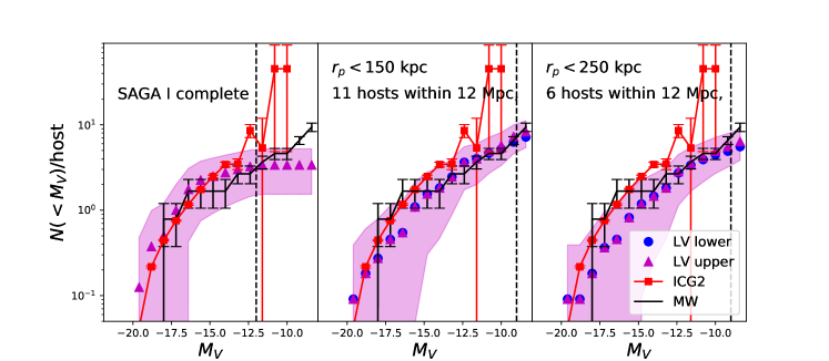
Figure 12: A comparison between the MW satellite LF and the satellite LFs of other MW-mass galaxies within 40 Mpc in the Local Volume (LV). Left: The comparison with the averaged satellite LF of eight MW-mass galaxies between 20 and 40 Mpc and from the SAGA survey (magenta triangles). Satellites are all confirmed and are complete out to $r_{p}\sim 300$ kpc to their central galaxies and down to $M_{V}\sim-12$. Middle: The comparison with the averaged satellite LF of eleven galaxies within 12 Mpc. Satellites are complete out to $r_{p}\sim 150$ kpc and down to $M_{V}\sim-9$. The blue dots and magenta triangles show the lower and upper limits when all unconfirmed satellites are treated as fore/background objects or as true satellites, respectively. Right: Similar to the middle panel, but shows a subset of six systems whose satellites are complete out to $r_{p}\sim 250$ kpc. In all panels, the black histograms are the MW satellite LF, whose errorbars are calculated in the same way as in previous plots. The magenta shaded regions are the Poisson errors for satellite LFs in the Local Volume, and this is not shown for blue dots, which have very similar errors. Red curves with errors are the averaged satellite LF of ICG2s, which is exactly the same as in Figure 7, and the errorbars are the 1-$\sigma$ scatters of 100 boot-strap subsamples, which reflect the errors on the averaged LF. An inner radius cut of 30 kpc has been adopted for all. The vertical black dashed lines mark the magnitudes beyond which the LV satellites are incomplete. By going down to $M_{V}\sim-9$, five more MW satellites (Carina, Leo II, Sextans, Draco I and Ursa Minor) are included, in addition to those summarised in Table LABEL:tbl:MWsat.

Table 5: A sample of MW-mass galaxies in the Local Volume and their properties, including the distance, projected separation out to which satellites are complete, stellar mass, halo mass estimated from satellite dynamics or abundance matching, number of satellites between 30 and 150 kpc in projection, and the reference from which we take the information of their satellites.

Name	$D$	1  $r_{\mathrm{comp}}$	$M_{V}$	$M_{\ast}$	$M_{\mathrm{halo}}$	2 $N_{\mathrm{sat}}(<M_{\mathrm{lim}},$	Source of
	[Mpc]	[kpc]		[$10^{10}M_{\odot}$]	[$10^{12}M_{\odot}$]	$30<r_{p}<150$ kpc)	satellites
3    M51	8.6	150	$-$21.38	$\sim$6	–	0–3	Carlsten et al. (2020c, a)
3    M64	5.3	300	$-$20.20	4.9	–	2	in preparation
3,8    M81	3.69	250	$-$21.10	$\sim$5	4.9$\pm$1.4	13	Chiboucas et al. (2013)
3,8    M101	6.52	300	$-$21.10	$\sim$4	1.5$\pm$0.7	8	Bennet et al. (2019, 2020)
							Javanmardi et al. (2016)
							Danieli et al. (2017)
							Carlsten et al. (2020b)
4    NGC4565	11.9	150	$-$21.80	7.6	–	3–8	Carlsten et al. (2020c, a)
3,8    NGC4258	7.2	150	$-$20.94	5.1	3.2$\pm$1.0	5	Carlsten et al. (2020c, a)
5,8    Centaurus A$\star$	3.77	200	$-$21.04	8.13	6.7$\pm$2.1	15	Müller et al. (2019)
							Karachentsev et al. (2007)
							Crnojević et al. (2019)
							Carlsten et al. (2020a)
3    NGC253	3.56	300	$-$20.10	7.2	–	1	in preparation
6,9    NGC1023	10.4	200	$-$20.90	7.7	$\sim$6	10–12	Carlsten et al. (2020c, a)
3    NGC5055	8.87	300	$-$21.10	4.9	–	7	in preparation
7    NGC6744	8.95	300	$-$21.62	6.6	–	5–6	in preparation
10    NGC5962	28.0	300	–	3.31	1.35	1	Geha et al. (2017)
10    NGC6181	34.3	300	–	3.72	1.86	3	Geha et al. (2017)
10    NGC5750	25.4	300	–	3.39	1.20	1	Geha et al. (2017)
10    NGC7716	34.8	300	–	5.01	1.02	1	Geha et al. (2017)
10    NGC1015	37.2	300	–	3.72	1.12	1	Geha et al. (2017)
10    PGC068743	39.2	300	–	3.63	1.51	2	Geha et al. (2017)
10    NGC2543	37.7	300	–	4.37	1.07	1	Geha et al. (2017)
10    NGC7541	37.0	300	–	5.13	3.55	5	Geha et al. (2017)

• Projected separation out to which the observed satellites are complete.

• We provide the number of satellites brighter than the limiting magnitude ($M_{V}\sim-12$ for SAGA galaxies and $M_{V}\sim-9$ for other more nearby galaxies) and projected between 30 and 150 kpc. In some systems, there are unconfirmed companions, and thus we provide the lower and upper boundaries.

• Stellar masses of M51, M64, M81, M101, NGC4258, NGC253 and NGC5055 are taken from the Spitzer Local Volume Legacy (LVL) Survey (Cook et al., 2014).

• Stellar mass of NGC4565 is taken from the Spitzer Survey of Stellar Structure in Galaxies (Sheth et al., 2010).

• Stellar mass of Centaurus A$\star$ is taken from Karachentsev & Kudrya (2014).

• Stellar mass of NGC1023 is estimated from the $K$-band absolute magnitude.

• Stellar mass of NGC6744 is taken from Yew et al. (2018).

• Halo mass computed from orbital motions of satellites (Karachentsev & Kudrya, 2014).

• Halo mass computed from satellite distribution (Trentham & Tully, 2009).

• Halo mass calculated from the $k$-band absolute magnitude and abundance matching.

While our MW is the Galaxy which we can study in the most detail, it is not straight-forward to measure its exact position on the colour-magnitude diagram, due to the fact that we are within the MW and is difficult to directly observe its global properties, and the observation is often strongly affected by dust reddening. A study by Licquia et al. (2015) picked up SDSS galaxies with similar stellar mass and star formation rates to our MW. After carefully correcting for Eddington bias and dust reddening, the photometric properties of these galaxies indicate that our MW locates at the “green valley”, which is a region sparsely populated by galaxies between the bimodel red and blue clouds of galaxies in the colour-magnitude diagram. Though a few earlier studies provide bluer colour estimates, the measurement by Licquia et al. (2015) is in good agreement with the novel measurement made by van der Kruit (1986) using the Galactic background light taken by the Pioneer 10 spacecraft. Similar to our MW, the colour of M31 also locates at the green valley region (e.g. Mutch et al., 2011).

Licquia et al. (2015) estimated the rest-frame colour of our MW as ${}^{0}(g-r)=0.682_{-0.056}^{+0.066}$. If the K-correction is made to $z=0.1$, which is the standard adopted in this paper, the rest-frame colour of our MW is about ${}^{0.1}(g-r)=0.822$. Therefore, the colour of our MW indeed almost lies on the line of colour division for red and blue galaxies, i.e., ${}^{0.1}(g-r)=0.065\log_{10}M_{\ast}/M_{\odot}+0.1$. For our sample of primaries, we have repeated the calculation for primaries with $0.722<^{0.1}(g-r)<0.922$ and with concentration, $C=R_{90}/R_{50}$, smaller than 2.6. Here the concentration parameter is adopted for a selection in morphology, so that the sample is dominated by low-concentration spiral galaxies. $R_{90}$ and $R_{50}$ are the 90% and 50% Petrosian radius, respectively. More details about the division by galaxy concentration can be found in D’Souza et al. (2014) and Wang et al. (2019). The averaged satellite LF of primaries selected in this way, though quite noisy due to the small number of galaxies in the green valley region, still tends to have steeper slopes and higher amplitudes at the faint end than the MW satellite LF.

A few early studies have investigated whether the global properties and scaling relations of our MW fits those of other galaxies, such as the Tully-Fisher relation (e.g. Flynn et al., 2006), the luminosity-velocity-radius relation (e.g. Licquia et al., 2016), star formation rate (e.g. Yin et al., 2009), [Fe/H] abundance, angular momentum (e.g. Hammer et al., 2007) and so on. Most of these studies report more than 1-$\sigma$ of deviation from the main relation, and thus the global properties of our MW are also uncommon compared with the majority of other spiral galaxies.

We conclude that the MW satellite LF is statistically atypical among other MW-mass galaxies. This is true unless the total stellar mass of our MW estimated by Licquia & Newman (2015), as used in our analysis, is much higher than the true value, or the stellar mass of other primary galaxies estimated from their photometric colours is significantly wrong. Due to the difficulties of measuring the global properties of our MW from inside, we cannot rule out such possibilities, but so far this is the best estimate we can have. As we have mentioned before, another independent study by McMillan (2011) provides a slightly larger value of MW stellar mass, $(6.43\pm 0.63)\times 10^{10}M_{\odot}$, which will lead to even higher amplitudes of extra-galactic satellite LFs at the faint end than that of our MW.

Therefore, we comment that it is dangerous to use satellites within our MW to represent the entire satellite population around galaxies with similar properties, as our MW is special compared with not only the average properties of other MW-mass galaxies, but is also statistically uncommon if taking into account the scatter. Comparing the averaged satellite property distributions from numerical simulations only with our MW is unfair, and we cannot draw strong cosmological implications without quoting the statistical uncertainties.

5.4 Satellite luminosity functions in the local volume

As we have mentioned in Section 1, despite the fact that the satellite LFs of other host galaxies within 40 Mpc tend to show large diversities, it was found in previous studies that our MW satellite LF is typical among other MW-mass galaxies in the local Universe. Thus in this subsection, we further make a detailed comparison between the satellite LF of our MW and of other MW-mass galaxies in the Local volume (LV).

A sample of 19 MW-mass galaxies in the LV is provided in Table LABEL:tbl:LVhost. Eight systems are taken from the first stage paper of the SAGA survey (Geha et al., 2017) out to $\sim$40 Mpc, and the satellites are complete down to $M_{V}\sim-12$. Eleven systems are within 12 Mpc, and the satellites are complete down to $M_{V}\sim-9$. Table LABEL:tbl:LVhost includes a few rich systems, such as M81, Centaurus A$\star$ and NGC1023. Their dark matter haloes, as estimated from satellite dynamics, tend to be more massive than that of our MW ($\sim 1\times 10^{12}M_{\odot}$, check Wang et al. (2020) for a review). Their stellar masses, on the other hand, are mostly within the mass range we adopt to select MW-mass galaxies ($10.63<\log_{10}M_{\ast}/M_{\odot}<10.93$), except for a few SAGA systems with $\log_{10}M_{\ast}<4\times 10^{10}M_{\odot}$. The magnitude gaps between central primaries and the brightest satellites of these galaxy systems satisfy our selection of ICG2s.

Figure 12 shows the comparison between the averaged satellite LFs of these LV systems and of our MW. Those observed by the SAGA survey and complete down to $M_{V}\sim-12$ are shown in the left panel. Those more nearby eleven systems within 12 Mpc are complete down to $M_{V}\sim-9$, while their satellites are complete out to different projected distances, $r_{\mathrm{comp}}$, but all systems are complete to 150 kpc. Thus in the middle panel we show the averaged satellite LF of all the eleven systems out to 150 kpc, and in the right panel, we show the averaged satellite LF for six out of the eleven systems, whose satellites are counted out to $r_{p}\sim$250 kpc. We also overplot the averaged satellite LF of ICG2s. The averaged LV satellite LFs tend to be more similar to the MW satellite LF, which is consistent with the recently submitted second stage SAGA results (Mao et al., 2020).

It seems the LF of satellites in our MW is more typical amongst the averaged satellite LF of MW-mass LV systems within 40 Mpc, but is more statistically uncommon amongst satellites of more distant MW-mass galaxies at redshift $z\sim 0.1$. Such an inconsistency might be connected to the so-called “local void”, that a large volume in the local Universe was reported to be deficient of galaxies (e.g. Tully, 1988; Peebles & Nusser, 2010). The local void can be predicted by numerical simulations, but is not extremely common, as Xie et al. (2014) reported that 11 out of 77 LG-like systems in the Millennium-II simulation have nearby low-density regions.

Guo et al. (2015b) reported that there are more satellites in filaments, and thus we can straight-forwardly think that central primary galaxies in over-dense regions tend to have more satellites. Similarly, we expect there are on average less satellites around central primaries in under-dense regions (or voids). Because the LV tends to be a “void” region, this can possibly explain why our MW satellites tend to be more typical in the LV, but the number of MW satellites with $M_{V}<-10$ tends to be less than the average of those around more distant galaxies.

However, we note that our statistical satellite counting methodology is quite different from that for the LV satellites, which confirms satellites through the line-of-sight distances. In addition, though the magnitude gaps between primaries and their secondary satellites of the LV systems satisfy our selection of ICG2s, the projected and line-of-sight separations adopted in the selection of ICG2s might not exactly fit the condition of these LV systems. Thus although as have been checked by Wang & White (2012) that the statistical satellite counts made in projection are $\sim$30% more than those made in 3-dimensional coordinates for MW-mass primaries, more detailed comparisons of the two satellite counting methodologies, including a careful investigation on the selection effects of spectroscopically confirmed satellites in the LV, and possible differences in the selection of primaries are still necessary. We leave them to future studies.

6 conclusion

In this study, we have measured the averaged satellite LFs of isolated central primary galaxies and galaxy pairs. Primary galaxies are selected from the SDSS spectroscopic Main galaxy sample. Satellites are constructed from the photometric source catalogues of HSC, DECaLS and SDSS. We compute the intrinsic luminosities of satellites following the method of Wang & White (2012), and fore/background source contaminations are statistically subtracted using the companion counts around random points.

Despite the very different depth, resolution, footprint, mode of observation and steps of data reduction, satellite LFs based on the three surveys agree very well with each other. Our measurements are also robust against the change in flux limits. We are not only able to extend previous measurements based on SDSS further down to the faint end by at most four magnitudes, but also we can measure the satellite LF around isolated central galaxies as small as $9.2<\log_{10}M_{\ast}/M_{\odot}<9.9$ and $8.5<\log_{10}M_{\ast}/M_{\odot}<9.2$, which are smaller than most of the previous studies based on similar methods. Our measurements can thus reach isolated central galaxies as small as the LMC, which predict an average number of 3–8 satellites brighter than $M_{V}\sim-10$ of LMC-mass systems.

We find both the bright end cutoff and the amplitude of satellite LFs over the whole luminosity range are sensitive to the magnitude gap between the central primary galaxy and its companions. A larger magnitude gap leads to more significant bright end cutoff by definition and also a decrease in the overall amplitude (or satellite abundance), indicating central primaries which have larger magnitude gaps than their secondary companions are hosted by less massive dark matter haloes.

In previous studies, it was reported that red central galaxies tend to have more satellites and are hosted by more massive dark matter haloes than blue central galaxies with the same stellar mass (e.g. Wang & White, 2012; Wang et al., 2014; Mandelbaum et al., 2016; Man et al., 2019). We fail to see such differences for red and blue primaries in pair, probably due to the small sample size and large errors, but by looking at galaxy pairs with different colour combinations, we find indications showing that galaxy pairs with red-red or blue-blue colour combinations have more satellites than red-blue galaxy pairs. However, such a trend for blue-blue pairs does not seem to be robust against changes in flux limits and might be affected by the sample variation at low redshifts, where the volume is small. And we fail to see similar trends in Illustris TNG-100.

By selecting central primary galaxies having similar stellar mass to our MW ($10.63<\log_{10}M_{\ast}/M_{\odot}<10.96$), we find at the bright end ($M_{V}<-16$), isolated central galaxies have on average 1.5–2.5 satellites, consistent with our MW. Satellite LFs around galaxies in pairs similar to the MW-M31 system tend to have slightly lower amplitudes at the bright end than the MW satellite LF.

We discover that the slopes of the averaged satellite LFs of both isolated central galaxies and galaxy pairs are steeper than that of MW satellites, and the amplitudes at $-15<M_{V}<-10$ are higher. The scatter of the satellite LFs predicted by numerical simulations can be quite large. Despite such a large scatter, the MW satellite LF at $M_{V}>-12$ still tends to be statistically uncommon. At such a bright magnitude range of MW satellites ($M_{V}<-10$), it is unlikely that there are other MW satellites remain undetected.

Therefore, we conclude that the LF of our MW satellites is atypical compared with those extra-galactic satellites around MW-mass central primaries. Interestingly, a comparison with 19 MW-mass systems in the Local Volume ($<$40 Mpc) reveals that the MW satellite LF is more typical among other systems in the LV, possibly implying the LV is an under-dense region (e.g. Tully, 1988; Peebles & Nusser, 2010). However, more detailed investigations on possible differences in the selection of primaries and the difference in satellite counting between systems in the nearby and the more distant Universe are still necessary in future studies.

Despite the much better agreement with LV systems, in order to have fair comparisons between real observations and theoretical predictions by modern numerical simulations, we can not use our MW to represent other MW-mass galaxies in the Universe, and thus the observation of faint satellites in extra-galactic systems are crucial for proper cosmological implications. Future deep and wide photometric surveys, such as the LSST survey (Ivezić et al., 2008) and the Chinese Space Station Optical Survey Telescope (CSST) is very promising to further extend the study of extra-galactic satellites down to much fainter magnitudes, and our statistical approach of studying faint photometric satellites around spectroscopic central primaries can be straight-forwardly applied to these future observations.

Data availability

The data in plots of this paper can be shared on reasonable request to the corresponding author.

Appendix A An inner radius cut to avoid source deblending mistakes

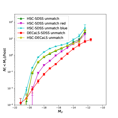
Figure 13: Green upper triangles connected by solid lines show the satellite LF based on extended sources detected in HSC but not in SDSS, and projected within 260 kpc to ICG1s with $11.63<\log_{10}M_{\ast}/M_{\odot}<11.93$. No inner radius cuts have been made. Magenta lower triangles/line and cyan stars/line show similar results, but are around red and blue ICG1s in the same stellar mass range separately. We also show satellite LF based on extended sources detected in DECaLS but not in SDSS as red dots/line, and the satellite LF using extended sources in HSC but not in DECaLS as yellow plus symbols/line. These sources which are detected in one survey but not in the other show very strong positive signals. Errorbars are based on the 1-$\sigma$ scatters of 100 boot-strap subsamples.

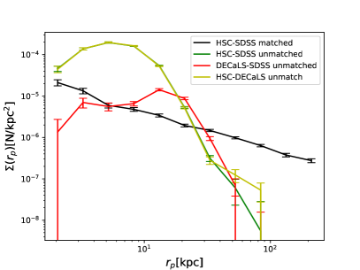
Figure 14: Green, red and yellow curves are the projected radial density profiles of extended sources detected in HSC but not in SDSS, in DECaLS but not in SDSS, and in HSC but not in DECaLS, respectively. The profiles are centred on ICG1s with $11.63<\log_{10}M_{\ast}/M_{\odot}<11.93$, and thus can be used to compare with symbols and lines with the same colour in Figure 13. The black curve shows the profile for extended sources which are detected in both HSC and SDSS. Extended sources in both DECaLS and SDSS (or in both HSC and DECaLS) have very similar projected radial density profiles as the black curve, and thus are not shown. The sources existing in one survey but not in the other tend to peak in the inner 20–30 kpc region. Errorbars are the 1-$\sigma$ scatters of 100 boot-strap subsamples.

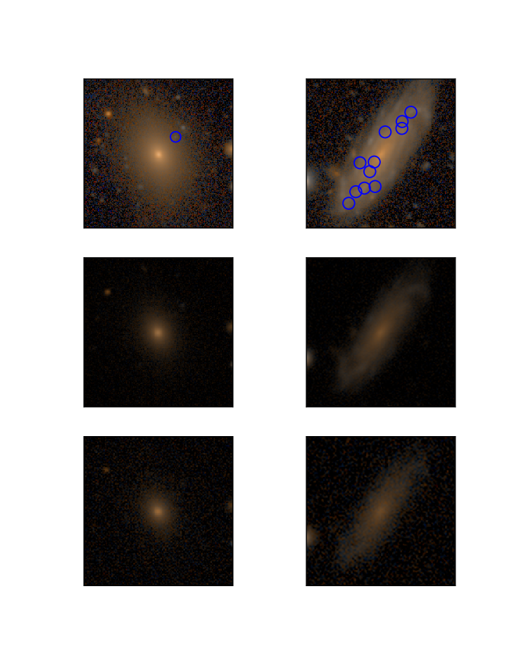
Figure 15: Image cutouts in RGB from HSC (top), DECaLS (middle) and SDSS (bottom), and centred on two example galaxies (two columns). In the top panels, blue circles mark extended sources which are not detected in DECaLS and SDSS. The half edge lengths of these image cutouts are 40 kpc. The colour mapping is exactly the same for all six panels. Because DECaLS does not have $i$-band observations, we choose $r$, ($g+r$)/2 and $g$ as inputs for the RGB mapping.

For results in the main text of this paper, we have applied an inner radius cut of $r_{p}>30$ kpc. In this Appendix we demonstrate the importance and the reason of choosing this inner radius cut by cross matching extended sources among HSC, DECaLS and SDSS. The matching also helps us to understand the difference among the three surveys.

We match extended sources with $r<21$ in one of the deeper surveys (HSC, DECaLS and HSC) correspondingly to all extended sources in another shallower surveys (SDSS, SDSS and DECaLS). The matching is based on a searching radius of 1$\arcsec$. Figure 13 shows the satellite LFs based on sources in a deeper survey, which do not have a match within 1$\arcsec$ in a corresponding shallower survey. For the plot, all companions within 260 kpc to the central primaries are included without any inner radius cut. The signals are clearly positive.

In order to investigate whether these sources detected in a deeper survey but not in another shallower survey are real, Figure 14 shows their projected radial density profiles after fore/background counts estimated from random points are subtracted. Compared with the profile of sources which exist in both HSC and SDSS, unmatched sources tend to peak in very inner regions. The signals are still positive beyond 30 kpc, but drop very quickly with the increase in $r_{p}$.

We further show the colour images containing such unmatched sources on small scales and centred on two example primary galaxies in Figure 15. The RGB figures are based on coadd images in $r$, ($g+r$)/2 and $g$-bands, and mapped to the RGB colour following the colour mapping of Lupton et al. (2004). It is very clear that with the greater depth and higher image resolution, HSC reveals more extended low surface brightness emissions around the central galaxy and resolves more substructures, such as the spiral arms and star forming regions along the arms. In the top right panel, we mark the extended sources which are failed to be detected in both HSC and DECaLS. These sources clearly trace the spiral arms, indicating they are not real satellite galaxies, but instead, they are part of the central primary galaxy, which are mistakenly deblended as companion sources. Such deblending mistakes are more frequently happening in HSC than those in SDSS and DECaLS. However, there are also examples showing that HSC is able to detect some more real sources. For example, in the top left panel, the source which exists in HSC but not in the other two surveys does look like a real one.

In fact, we have looked at many image cutouts centred on our primary galaxies, and with different image sizes. Most of the sources close to the central galaxy, in a deeper survey but not in another shallower survey are faked detections due to deblending mistakes, and this often happens around bluer spiral galaxies, though there are also examples of real detections such as the one in the top left panel of Figure 15.

Magenta lower triangles/line and cyan stars/line in Figure 13 can prove and summarise what we have seen. The cyan stars connected by lines show satellite LFs based on extended sources in HSC but not in SDSS and around blue primaries. On the other hand, the magenta triangles connected by lines show similar results around red primaries. The amplitude of the cyan curve is much higher than the magenta one, indicating there are more such sources around blue galaxies. Blue star forming galaxies have more rich substructures, which are more likely to be mistakenly deblended as companions sources.

Because such faked sources mostly exist within $r_{p}\sim$30 kpc according to Figure 14, we choose an inner radius cut of 30 kpc for all the results in the main text of this paper. Such an inner radius cut, of course, would also exclude real sources on small scales, but by applying this cut to all of the three surveys and also to MW satellites after accounting for the projection effect (see Section 3 for details), we can ensure that our comparisons among different surveys and the comparison with MW satellites are fair. Beyond 30 kpc, such sources still exist, but as the readers can see form Figure 14, even if all these sources are faked, they are subdominant and are unlikely to significantly affect our results. In fact, we have looked into such sources in HSC on larger distances to the central primaries, and have found examples that look like real galaxies. This can at least partly explain why satellite LFs based on HSC tend to have slightly higher amplitudes than those based on SDSS or DECaLS in the main text.

Besides, the central primary may have another apparent massive companion galaxy close to it in projection, but it is in fact not physically associated because they have very different spectroscopic redshifts. There can be some faked sources around this massive companion galaxy, which are detected due to deblending mistakes, contributing to the number of unmatched sources. We expect the probabilities for such cases to happen are equivalent around real central primaries and around random points. As a result, they should have been subtracted by using satellite counts around random points and thus are not expected to affect our results. However, if a true late-type satellite galaxy, that has a projected separation larger than 30 kpc to the central primary and is mistakenly deblended into multiple sources, the amplitude of our measured satellite LFs can be increased in a wrong way. We cannot rule out such possibilities and it is not trivial to estimate the exact fractions, but we believe our conclusions are unlikely to have been significantly affected, based on the fact that HSC is only slightly higher in amplitude than both DECaLS and SDSS.

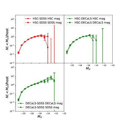
Figure 16: Satellite LFs based on matched extended sources between HSC and SDSS, between HSC and DECaLS, and between DECaLS and SDSS. For each set, two different types of magnitudes taken from either of the two surveys are used.

In addition to the unmatched sources, we also use the matched sources between different surveys to investigate whether the different magnitudes and filter systems defined in HSC, DECaLS and SDSS can lead to significant discrepancies. This is shown in Figure 16. The three panels correspond to matched extended sources in HSC-SDSS, HSC-DECaLS and DECaLS-SDSS, respectively. In each panel, the solid and dashed curves are results based on magnitudes from either of the two surveys. We can see some small differences at faint magnitudes, but the differences are far from being large enough to affect the conclusions of this paper.

References

- Abazajian et al. (2009) Abazajian K. N., et al., 2009, ApJS, 182, 543
- Aihara et al. (2011) Aihara H., et al., 2011, ApJS, 193, 29
- Aihara et al. (2018a) Aihara H., Arimoto N., Armstrong R., Arnouts S., Bahcall N. A., Bickerton S., Bosch J., Bundy K., 2018a, PASJ, 70, S4
- Aihara et al. (2018b) Aihara H., Armstrong R., Bickerton S., Bosch J., Coupon J., Furusawa H., Hayashi Y., Ikeda H., 2018b, PASJ, 70, S8
- Angulo & White (2010) Angulo R. E., White S. D. M., 2010, MNRAS, 405, 143
- Bechtol et al. (2015) Bechtol K., et al., 2015, ApJ, 807, 50
- Belokurov et al. (2010) Belokurov V., et al., 2010, ApJ, 712, L103
- Bennet et al. (2019) Bennet P., Sand D. J., Crnojević D., Spekkens K., Karunakaran A., Zaritsky D., Mutlu-Pakdil B., 2019, ApJ, 885, 153
- Bennet et al. (2020) Bennet P., Sand D. J., Crnojević D., Spekkens K., Karunakaran A., Zaritsky D., Mutlu-Pakdil B., 2020, ApJ, 893, L9
- Benson et al. (2002a) Benson A. J., Lacey C. G., Baugh C. M., Cole S., Frenk C. S., 2002a, MNRAS, 333, 156
- Benson et al. (2002b) Benson A. J., Frenk C. S., Lacey C. G., Baugh C. M., Cole S., 2002b, MNRAS, 333, 177
- Bertin (2011) Bertin E., 2011, in Evans I. N., Accomazzi A., Mink D. J., Rots A. H., eds, Astronomical Society of the Pacific Conference Series Vol. 442, Astronomical Data Analysis Software and Systems XX. p. 435
- Blakeslee et al. (2009) Blakeslee J. P., et al., 2009, ApJ, 694, 556
- Blanton & Roweis (2007) Blanton M. R., Roweis S., 2007, AJ, 133, 734
- Blanton et al. (2005) Blanton M. R., et al., 2005, AJ, 129, 2562
- Bosch et al. (2018) Bosch J., et al., 2018, PASJ, 70, S5
- Boylan-Kolchin et al. (2009) Boylan-Kolchin M., Springel V., White S. D. M., Jenkins A., Lemson G., 2009, MNRAS, 398, 1150
- Boylan-Kolchin et al. (2010) Boylan-Kolchin M., Springel V., White S. D. M., Jenkins A., 2010, MNRAS, 406, 896
- Boylan-Kolchin et al. (2011a) Boylan-Kolchin M., Besla G., Hernquist L., 2011a, MNRAS, 414, 1560
- Boylan-Kolchin et al. (2011b) Boylan-Kolchin M., Bullock J. S., Kaplinghat M., 2011b, MNRAS, 415, L40
- Bullock et al. (2000) Bullock J. S., Kravtsov A. V., Weinberg D. H., 2000, ApJ, 539, 517
- Busha et al. (2011) Busha M. T., Wechsler R. H., Behroozi P. S., Gerke B. F., Klypin A. A., Primack J. R., 2011, ApJ, 743, 117
- Callingham et al. (2019) Callingham T. M., et al., 2019, MNRAS, 484, 5453
- Cantiello et al. (2018) Cantiello M., et al., 2018, ApJ, 856, 126
- Carlsten et al. (2019) Carlsten S. G., Beaton R. L., Greco J. P., Greene J. E., 2019, ApJ, 879, 13
- Carlsten et al. (2020a) Carlsten S. G., Greene J. E., Peter A. H. G., Beaton R. L., Greco J. P., 2020a, arXiv e-prints, p. arXiv:2006.02443
- Carlsten et al. (2020b) Carlsten S. G., Greene J. E., Peter A. H. G., Greco J. P., Beaton R. L., 2020b, arXiv e-prints, p. arXiv:2006.02444
- Carlsten et al. (2020c) Carlsten S. G., Greco J. P., Beaton R. L., Greene J. E., 2020c, ApJ, 891, 144
- Cautun et al. (2014a) Cautun M., Frenk C. S., van de Weygaert R., Hellwing W. A., Jones B. J. T., 2014a, MNRAS, 445, 2049
- Cautun et al. (2014b) Cautun M., Hellwing W. A., van de Weygaert R., Frenk C. S., Jones B. J. T., Sawala T., 2014b, MNRAS, 445, 1820
- Cautun et al. (2015) Cautun M., Wang W., Frenk C. S., Sawala T., 2015, MNRAS, 449, 2576
- Cautun et al. (2019) Cautun M., Deason A. J., Frenk C. S., McAlpine S., 2019, MNRAS, 483, 2185
- Cautun et al. (2020) Cautun M., et al., 2020, MNRAS, 494, 4291
- Chabrier (2003) Chabrier G., 2003, PASP, 115, 763
- Chambers et al. (2016) Chambers K. C., et al., 2016, arXiv e-prints, p. arXiv:1612.05560
- Chiboucas et al. (2013) Chiboucas K., Jacobs B. A., Tully R. B., Karachentsev I. D., 2013, AJ, 146, 126
- Cook et al. (2014) Cook D. O., et al., 2014, MNRAS, 445, 899
- Crnojević et al. (2019) Crnojević D., et al., 2019, ApJ, 872, 80
- Cunha et al. (2009) Cunha C. E., Lima M., Oyaizu H., Frieman J., Lin H., 2009, MNRAS, 396, 2379
- D’Onghia & Lake (2008) D’Onghia E., Lake G., 2008, ApJ, 686, L61
- D’Souza et al. (2014) D’Souza R., Kauffman G., Wang J., Vegetti S., 2014, MNRAS, 443, 1433
- Danieli et al. (2017) Danieli S., van Dokkum P., Merritt A., Abraham R., Zhang J., Karachentsev I. D., Makarova L. N., 2017, ApJ, 837, 136
- Danieli et al. (2018) Danieli S., van Dokkum P., Conroy C., 2018, ApJ, 856, 69
- Deason et al. (2015) Deason A. J., Wetzel A. R., Garrison-Kimmel S., Belokurov V., 2015, MNRAS, 453, 3568
- Dey et al. (2019) Dey A., et al., 2019, AJ, 157, 168
- Dooley et al. (2017) Dooley G. A., Peter A. H. G., Carlin J. L., Frebel A., Bechtol K., Willman B., 2017, MNRAS, 472, 1060
- Drlica-Wagner et al. (2015) Drlica-Wagner A., et al., 2015, ApJ, 813, 109
- Eadie et al. (2015) Eadie G. M., Harris W. E., Widrow L. M., 2015, ApJ, 806, 54
- Flaugher et al. (2015) Flaugher B., et al., 2015, AJ, 150, 150
- Flynn et al. (2006) Flynn C., Holmberg J., Portinari L., Fuchs B., Jahreiß H., 2006, MNRAS, 372, 1149
- Fukugita et al. (1996) Fukugita M., Ichikawa T., Gunn J. E., Doi M., Shimasaku K., Schneider D. P., 1996, AJ, 111, 1748
- Furusawa et al. (2018) Furusawa H., et al., 2018, PASJ, 70, S3
- Garrison-Kimmel et al. (2019) Garrison-Kimmel S., et al., 2019, MNRAS, 487, 1380
- Geha et al. (2017) Geha M., et al., 2017, ApJ, 847, 4
- Gnedin et al. (2010) Gnedin O. Y., Brown W. R., Geller M. J., Kenyon S. J., 2010, ApJ, 720, L108
- González et al. (2013) González R. E., Kravtsov A. V., Gnedin N. Y., 2013, ApJ, 770, 96
- Gunn et al. (1998) Gunn J. E., et al., 1998, AJ, 116, 3040
- Gunn et al. (2006) Gunn J. E., et al., 2006, AJ, 131, 2332
- Guo et al. (2010) Guo Q., White S., Li C., Boylan-Kolchin M., 2010, MNRAS, 404, 1111
- Guo et al. (2011a) Guo Q., et al., 2011a, MNRAS, 413, 101
- Guo et al. (2011b) Guo Q., Cole S., Eke V., Frenk C., 2011b, MNRAS, 417, 370
- Guo et al. (2013) Guo Q., White S., Angulo R. E., Henriques B., Lemson G., Boylan-Kolchin M., Thomas P., Short C., 2013, MNRAS, 428, 1351
- Guo et al. (2015a) Guo Q., Cooper A. P., Frenk C., Helly J., Hellwing W. A., 2015a, MNRAS, 454, 550
- Guo et al. (2015b) Guo Q., Tempel E., Libeskind N. I., 2015b, ApJ, 800, 112
- Hammer et al. (2007) Hammer F., Puech M., Chemin L., Flores H., Lehnert M. D., 2007, ApJ, 662, 322
- Hargis et al. (2014) Hargis J. R., Willman B., Peter A. H. G., 2014, ApJ, 795, L13
- Henriques et al. (2015) Henriques B. M. B., White S. D. M., Thomas P. A., Angulo R., Guo Q., Lemson G., Springel V., Overzier R., 2015, MNRAS, 451, 2663
- Homma et al. (2018) Homma D., et al., 2018, PASJ, 70, S18
- Homma et al. (2019) Homma D., et al., 2019, PASJ, 71, 94
- Irwin et al. (2007) Irwin M. J., et al., 2007, ApJ, 656, L13
- Ivezić et al. (2008) Ivezić Ž., et al., 2008, preprint, (arXiv:0805.2366)
- Ivezić et al. (2019) Ivezić Ž., et al., 2019, ApJ, 873, 111
- Javanmardi et al. (2016) Javanmardi B., et al., 2016, A&A, 588, A89
- Jee & Tyson (2011) Jee M. J., Tyson J. A., 2011, PASP, 123, 596
- Jethwa et al. (2016) Jethwa P., Erkal D., Belokurov V., 2016, MNRAS, 461, 2212
- Jiang et al. (2012) Jiang C. Y., Jing Y. P., Li C., 2012, ApJ, 760, 16
- Jurić et al. (2017) Jurić M., et al., 2017, in Lorente N. P. F., Shortridge K., Wayth R., eds, Astronomical Society of the Pacific Conference Series Vol. 512, Astronomical Data Analysis Software and Systems XXV. p. 279 (arXiv:1512.07914)
- Kallivayalil et al. (2006) Kallivayalil N., van der Marel R. P., Alcock C., 2006, ApJ, 652, 1213
- Karachentsev & Kudrya (2014) Karachentsev I. D., Kudrya Y. N., 2014, AJ, 148, 50