Recent scaling properties of Bitcoin price returns

Abstract

While relevant stylized facts are observed for Bitcoin markets, we find a distinct property for the scaling behavior of the cumulative return distribution. For various assets, the tail index $\mu$ of the cumulative return distribution exhibits $\mu\approx 3$, which is referred to as ”the inverse cubic law.” On the other hand, that of the Bitcoin return is claimed to be $\mu\approx 2$, which is known as ”the inverse square law.” We investigate the scaling properties using recent Bitcoin data and find that the tail index changes to $\mu\approx 3$, which is consistent with the inverse cubic law. This suggests that some properties of the Bitcoin market could vary over time. We also investigate the autocorrelation of absolute returns and find that it is described by a power-law with two scaling exponents. By analyzing the absolute returns standardized by the realized volatility, we verify that the Bitcoin return time series is consistent with normal random variables with time-varying volatility.

1 Introduction

In 2008, Nakamoto[1] proposed Bitcoin as the first practical cryptocurrency based on the blockchain technology. His proposal was quickly accepted, and in 2009, the Bitcoin network was launched as a peer-to-peer payment network. Since then, a number of digitized cryptocurrencies have been proposed and created, and growing cryptocurrency markets have a strong impact on contemporary financial markets. Bitcoin has recently attracted the interest of researchers and various properties and aspects of Bitcoin have been investigated. For example, volatility analysis [2, 3], price clustering[4, 5], adaptive market hypothesis [6], transaction activity [7], multifractality[8], liquidity and efficiency[9], Taylor effect[10], structural breaks [11], long memory effects[12], rough volatility[13], power-law cross-correlation[14], asymmetric multifractal analysis[15], and so forth.

Universal properties across various financial time series are classified as stylized facts[16], which include (i) fat-tailed distributions, (ii) volatility clustering, and (iii) slow decay of autocorrelation in absolute returns, among others. While stylized facts are also observed in Bitcoin, for example, [17, 8], a distinct property has been observed for the tail index of return distributions. For other assets such as stocks, it is known that the tail of the cumulative return distribution is described by a power-law function and its tail index $\mu$ is obtained as $\mu\approx 3$, known as ”the inverse cubic law”[18, 19, 20, 21]. For the Bitcoin market before 2014, the tail index is estimated to be $\mu\approx 2$, which differs from the known stylized fact for other assets and is referred to as ”the inverse square law”[22]. Similar tail indices have also been reported in Ref.[23]. Since this is a newly emerging market, market properties of Bitcoin could change as trading activity increases over time. In fact, the market efficiency measured by the Hurst exponent of the return time series varies over time and at the early stage of the Bitcoin market, the Hurst exponent is observed to be less than 1/2, which indicates that the time series is anti-persistent[24]. This anti-persistent behavior could be related to the illiquidity of the Bitcoin market[9, 25]. As the liquidity of the Bitcoin market improves, the Hurst exponent moves to 1/2[24, 25].

We investigate the possible change in scaling properties of the return distribution for the recent Bitcoin market. We also investigate the cumulative distributions and autocorrelation of the absolute returns and the return standardized by the realized volatility.

2 Data set

The data are Bitcoin tick data (in dollars) traded on Bitstamp from September 11, 2011 to June 21, 2020 and downloaded from Bitcoincharts. We construct 1-min price data from the Bitcoin tick data and then calculate 1-min returns $R_{t},t=1,2,...,N$ as

$$R_{t}=\log p_{t}-\log p_{t-1},$$ (1)

where $p_{t}$ is the 1-min price at $t$ (min). We further standardize the returns data using

$${\bar{R_{t}}}=\frac{R_{t}-\nu}{\sigma}.$$ (2)

where $\nu$ and $\sigma$ represent the average and standard deviation of returns $R_{t}$, respectively. We select the following two data periods from the data, which separate low and high liquidity periods: I) September 11, 2011-December 31, 2013 and II) January 1, 2015-June 21, 2020. Dataset I (II) contains low (high) liquidity data[25].

3 Results

First, we show the cumulative distributions of returns in Figure 1(a): positive tail and (b): negative tail, in a log-log plot, and recognize that the tail behavior is described by a power law. While there is no significant difference between positive and negative tails, a considerable difference is seen between data periods, that is, a heavier tail is observed for the cumulative distribution of dataset (II), which contains high liquidity data. We obtain tail indices of the cumulative distributions by a regression fit to a power-law function of $\kappa\bar{R}^{-\mu}$, where $\kappa$ and $\mu$ are fitting parameters. The results of the tail indices are reported in Table 1. The tail index for dataset I is $\mu\approx 2$, which is consistent with the previous results obtained for earlier periods[22]. On the other hand, the tail index for II is $\mu\approx 3$, which is consistent with the tail index obtained for other assets such as stocks. For the entire data set, we find a tail index between I and II. Our findings suggest that the scaling properties of the return distributions of the Bitcoin market could change over time, For the recent liquidity of the Bitcoin market, the tail index is in agreement with the well-known stylized facts for other assets.

Table 1: Results of tail index.

	(I) 2011-2013	(II) 2015-2020	2011-2020
Fitting region	[2,20]	[2,20]	[1,10]
positive tail index $\mu$	-2.06	-3.33	-2.35
negative tail index $\mu$	-2.08	-3.23	-2.38

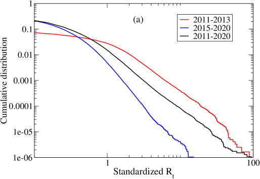
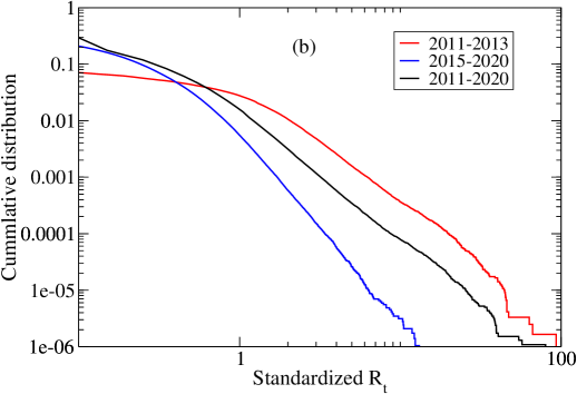
Figure 1: (a) Cumulative distribution for positive tail. (b) Cumulative distribution for negative tail.

Next, we show the autocorrelation function (ACF) of the absolute returns. The ACF of a time series $x_{i}:i=1,...,N$ is defined by

$$ACF(t)=\frac{\langle(x_{i}-\rho)(x_{i+j}-\rho)\rangle}{\sigma_{x}^{2}}.$$ (3)

where $\rho$ and $\sigma_{x}^{2}$ represent the average and variance of $x_{i}$, respectively, and $\langle O_{i}\rangle$ means taking an average over $O_{i}$. Figure 2 displays the ACF of the absolute returns in the log-log plot and we see that the ACF is also well described by a power law. A remarkable characteristic of the ACF is that the power-law exponent seems to change at $t\sim 1000$. The power-law exponent for $t>1000$ is found to be larger than that for $t<1000$. There is no clear explanation for this change. The results of the power-law exponents are reported in Table 2. Furthermore, we find that there is no substantial difference for the power-law exponents between the three data sets. Thus, the long-memory property of Bitcoin remains unchanged over time.

Table 2: Results of the power-law exponent.

	(I) 2011-2013	(II) 2015-2020	2011-2020
fitting region	[3,500]	[3,500]	[3,500]
exponent $\mu$	-0.121	-0.116	-0.120
fitting region	[15000,10000]	[1500,10000]	[1500,10000]
exponent $\mu$	-0.197	-0.235	-0.206

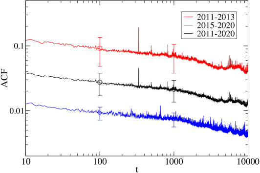
Figure 2: ACF of absolute returns. The symbols at t=100 and 1000 show typical one-sigma errors calculated using the jackknife method.

The power law observed in the absolute return means that the time series of the absolute return has long memory, which sharply contrasts to returns for which the ACF of the return time series is short ranged. The long memory in the absolute returns is considered to be related to the time correlation of volatility. Let us assume that the return time series is described by $R_{t}\equiv\sigma_{t}\epsilon_{t}$, where $\sigma_{t}$ is the volatility at $t$ and $\epsilon_{t}$ is the standard normal random variable. Namely, the return $R_{t}$ is assumed to behave as a normal random variable with time-varying volatility. This assumption of returns automatically satisfies no autocorrelation in returns. On the other hand, the autocorrelation of absolute returns depends on the time structure of $\sigma_{t}$. If we standardize the (observed) returns $R_{t}$ by $\sigma_{t}$, that is, $R_{t}/\sigma_{t}\equiv\tilde{R_{t}}$, we expect to obtain the standard normal random time series $\epsilon_{t}$. To test whether $\tilde{R_{t}}$ satisfies this expectation we need to estimate the volatility $\sigma_{t}$ of returns in the proper manner because volatility is not observable in the financial markets.

In empirical finance, the standard technique to estimate volatility is to use volatility models such as GARCH-type models[26, 27, 28, 29, 30, 31, 32, 33]. The drawback of using such models is that volatility estimates are model-dependent, and which estimate is better is not well defined. Recent availability of high-frequency financial data enable us to obtain a model-free estimate known as ”realized volatility (RV)”[34, 35] constructed by the sum of the square of intraday returns. The returns standardized by the RV are examined for the exchange rate[36, 37] and return[38], and the normality of the standardized return $\tilde{R_{t}}$ is established. However, detailed studies report the existence of deviation from the normality caused by the low sampling frequency in the RV[39, 40, 41, 42, 43]. Furthermore because $\tilde{R_{t}}$ is expected to be a random variable, we should observe no autocorrelation not only for $\tilde{R_{t}}$ but also for the absolute $\tilde{R_{t}}$, that is, $|\tilde{R_{t}}|$. The autocorrelation of the absolute $\tilde{R_{t}}$ is examined for Japanese stocks[44], and it is verified that no autocorrelation is observed for the absolute $\tilde{R_{t}}$. We examine the nonexistence of autocorrelation in the absolute $\tilde{R_{t}}$ of Bitcoin. Figure 3 shows the autocorrelation of the absolute $\tilde{R_{t}}$ standardized by the RV at a 5-min sampling frequency, and we confirm that there is no significant autocorrelation in the absolute $\tilde{R_{t}}$.

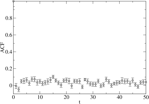
Figure 3: ACF of the absolute returns standardized by RV. For the calculation of the ACF, we take the data from January 10, 2015 to June 21, 2020.

4 Conclusions

We investigate the scaling properties of the Bitcoin market and find that the tail index $\mu$ of the cumulative return distribution changes from $\mu\approx 2$ to $\mu\approx 3$, which indicates that the recent Bitcoin market exhibits the well-established scaling law, that is, the inverse cubic law. Our findings suggest that some properties of the Bitcoin market could change over time.

We find that the autocorrelation of absolute returns shows a power law with two scaling exponents separated at approximately $t=1000$min. The ACF of the absolute returns standardized by RV shows no autocorrelation, which indicates that the return time series is consistent with a normal random variable with time-varying volatility.

References

References

- [1] Nakamoto S 2008 Bitcoin: A peer-to-peer electronic cash system https://bitcoin.org/bitcoin.pdf
- [2] Bouoiyour J and Selmi R 2016 Economics Bulletin 36 1430–1440
- [3] Dyhrberg A H 2016 Finance Research Letters 16 85–92
- [4] Urquhart A 2017 Economics Letters 159 145–148
- [5] Li X, Li S and Xu C 2018 Finance Research Letters
- [6] Khuntia S and Pattanayak J 2018 Economics Letters 167 26–28
- [7] Koutmos D 2018 Economics Letters 167 81–85
- [8] Takaishi T 2018 Physica A 506 507–519
- [9] Wei W C 2018 Economics Letters 168 21–24
- [10] Takaishi T and Adachi T 2018 Economics Letters 172 5–7
- [11] Thies S and Molnár P 2018 Finance Research Letters 27 223–227
- [12] Phillip A, Chan J and Peiris S 2019 Finance Research Letters 28 95–100
- [13] Takaishi T 2020 Finance Research Letters 32 101379
- [14] Takaishi T 2020 EPL (Europhysics Letters) 129 28001
- [15] Kristjanpoller W, Bouri E and Takaishi T 2020 Physica A 545 123711
- [16] Cont R 2001 Quantitative Finance 1 223–236
- [17] Chu J, Chan S, Nadarajah S and Osterrieder J 2017 Journal of Risk and Financial Management 10 17
- [18] Gopikrishnan P, Meyer M, Amaral L N and Stanley H E 1998 The European Physical Journal B-Condensed Matter and Complex Systems 3 139–140
- [19] Gopikrishnan P, Plerou V, Amaral L A N, Meyer M and Stanley H E 1999 Physical Review E 60 5305
- [20] Plerou V, Gopikrishnan P, Amaral L A N, Meyer M and Stanley H E 1999 Physical review E 60 6519
- [21] Pan R K and Sinha S 2007 EPL (Europhysics Letters) 77 58004
- [22] Easwaran S, Dixit M and Sinha S 2015 Econophysics and data driven modelling of market dynamics (Springer) pp 121–128
- [23] Begušić S, Kostanjčar Z, Stanley H E and Podobnik B 2018 Physica A 510 400–406
- [24] Urquhart A 2016 Economics Letters 148 80–82
- [25] Takaishi T and Adachi T 2020 Asia-Pacific Financial Markets 27 145–154
- [26] Engle R F 1982 Econometrica: Journal of the Econometric Society 987–1007
- [27] Bollerslev T 1986 Journal of Econometrics 31 307–327
- [28] Glosten L, Jaganathan R and Runkle D 1993 Journal of Finance 48 1779–1801
- [29] Nelson D 1991 Econometrica 59 347–370
- [30] Sentana E 1995 Review of Economic Studies 62 639–661
- [31] Takaishi T 2017 Physica A 473 451–460
- [32] Takaishi T 2018 Quantitative Finance and Economics 2 127–36
- [33] Bollerslev T, Chou R Y and Kroner K F 1992 Journal of econometrics 52 5–59
- [34] Andersen T G and Bollerslev T 1998 International economic review 885–905
- [35] McAleer M and Medeiros M C 2008 Econometric Reviews 27 10–45
- [36] Andersen T G, Bollerslev T, Diebold F X and Labys P 2000 Multinational Finance Journal 4 159–179
- [37] Andersen T G, Bollerslev T, Diebold F X and Labys P 2001 Journal of the American statistical association 96 42–55
- [38] Andersen T G, Bollerslev T, Diebold F X and Ebens H 2001 Journal of financial economics 61 43–76
- [39] Andersen T G, Bollerslev T and Dobrev D 2007 Journal of Econometrics 138 125–180
- [40] Takaishi T 2012 Procedia-Social and Behavioral Sciences 65 968–973
- [41] Takaishi T 2014 JPS Conf. Proc. 1 019007
- [42] Takaishi T and Watanabe T 2016 Journal of Physics: Conference Series 710 012010
- [43] Takaishi T 2018 Physica A 500 139–154
- [44] Takaishi T, Chen T T and Zheng Z 2012 Progress of Theoretical Physics Supplement 194 43–54
- [45] Takaishi T 2013 Journal of Physics: Conference Series 454 012041
- [46] Bandi F M and Russell J R 2006 Journal of Financial Economics 79 655–692
- [47] Liu L Y, Patton A J and Sheppard K 2015 Journal of Econometrics 187 293–311