Solitary wave solutions of the 2+1 and 3+1 dimensional nonlinear Dirac equation constrained to planar and space curves

Abstract

We study the effect of curvature and torsion on the solitons of the nonlinear Dirac equation considered on planar and space curves. Since the spin connection is zero for the curves considered here, the arc variable provides a natural setting to understand the role of curvature and then we can obtain the transformation for the 1+1 dimensional Dirac equation directly from the metric. Depending on the curvature, the soliton profile either narrows or expands. Our results may be applicable to yet-to-be-synthesized curved quasi-one dimensional Bose condensates.

I Introduction

Recently there has been renewed interest in the nonlinear Dirac equation (NLDE) because it arises in Bose condensation in honeycomb optical lattices where confining potentials allow for quasi-one dimensional (Q1D) confinement Haddad . Here we show that one can find exact solitary wave solutions for the Dirac equation confined to various space curves by using either the arc variable representation or the vierbein formalism of Weyl Weyl . The latter is elucidated in the Appendix. We find that since the curves are only in the spatial part of the metric, one can transform the NLDE on the curved surface to another flat space NLDE by a coordinate transformation. This allows us to obtain the solutions of the Dirac equation analytically for the conic surfaces such as a hyperbola or parabola as well as helical (space) curves in 3+1 dimensions in terms of the spatial arc length parameter s. One can furthermore analytically obtain the connection between the parametric description of the curve and the spatial arc length variable s.

To our knowledge there are no studies of NLD solitons in curved geometries either experimentally or theoretically. However, one could envision constructing curved QID Bose condensates, which serves as one of our motivations. In contrast, solitons and breathers have been studied on curves in the context of the nonlinear Schrödinger (NLS) equation Gaididei ; Tsironis with an interesting interplay of curvature and nonlinearity through the soliton/breather solutions. The study of nonlinear waves on curves and closed surfaces is important in its own right ludu .

This paper is structured as follows. In the next section we study the NLD equation on conic sections such as a hyperbola, parabola and ellipse. In section III we show how the normalized charge density of a soliton is modified due to the curvature. In section IV we consider Jacobi elliptic and other parameterizations of the various curves. Section V deals with space curves (i.e. with finite torsion) such as a helix, an elliptic helix and the helix of the hyperboloid of revolution. Finally in section VI we provide our main conclusions.

II Nonlinear Dirac equation constrained to space curves in $2+1$ dimensions

First let us consider the solutions of the Nonlinear Dirac Equation (NLD equation) in $2+1$ dimensions (often called the Gross-Neveu model ref:GN ) when it is confined to a conic section which is a hyperbola, ellipse or parabola. The NLD equation including a mass term is given by:

$$-i(\gamma^{\mu}\partial_{\mu}+m)\Psi-g^{2}(\bar{\Psi}\Psi)\Psi=0\,,$$ (1)

where $\gamma^{\mu}$ are Dirac matrices. It will be convenient in studying the transformation properties of this equation to introduce the quantity $\sigma$

$$\sigma\equiv-i{g^{2}}\bar{\Psi}\Psi,$$ (2)

so that we can rewrite the NLD equation in the suggestive form often used in the large-N type expansions of the quantum version of this theory

$$-i[\gamma^{\mu}\partial_{\mu}+(m+\sigma)]\Psi=0.$$ (3)

The fact that $\sigma$ transforms as a scalar is what will be important in what follows.

II.1 Hyperbola

First let us consider the hyperbola defined by $y^{2}-x^{2}=a^{2}$. Here $\eta$ is an azimuthal angle. The parametrization

$$y=a\sec u,~{}~{}~{}x=a\tan u,$$ (4)

with $-\pi/2<u<\pi/2$, fulfills this condition. We have that

$$ds^{2}=dx^{2}+dy^{2}=\left[a^{2}\sec^{2}(u)\left(\tan^{2}(u)+\sec^{2}(u)\right)\right]du^{2}.$$ (5)

If we introduce a new coordinate via $d\textbf{s}=ds=a\sec(u)\sqrt{\tan^{2}(u)+\sec^{2}(u)}du$, which is the arc length along the curve, we can solve the usual Dirac equation in terms of s and then use the relationship:

$$\textbf{s}[a,u]=a(\sec(u)\sqrt{\tan^{2}(u)+\sec^{2}(u)}-1)$$ (6)

to obtain the solutions as a function of $u,t$, The resulting 1+1 dimensional NLD equation is

$$(\gamma^{0}\partial_{t}+\gamma^{1}\partial_{\textbf{s}}+\sigma+m)\Psi[\textbf{s},t]=0.$$ (7)

We see that because the spin connection is zero, one could have obtained this answer by realizing that the metric

$$(ds)^{2}=-(dt)^{2}+(dx)^{2}+(dy)^{2}=-(dt)^{2}+a^{2}\sec^{2}(u)\left(\tan^{2}(u)+\sec^{2}(u)\right)du^{2}\,.$$ (8)

The 2+1 dimensional metric can be transformed to a $1+1$ dimensional Minkowski metric by the transformation

$$ds=a\sec(u)\sqrt{\tan^{2}(u)+\sec^{2}(u)}du$$ (9)

Then we would obtain the solutions of the NLD equation as a function of $\textbf{s},t$ and then obtain the result in terms of $u$ using $\textbf{s}[u]$. The 1+1 dimensional resulting NLDE is translationally invariant under $\textbf{s}\rightarrow\textbf{s}-\textbf{s}_{0}$, so there are solitary wave solutions centered at any value of the arc length $\textbf{s}_{0}$.

Note that if the transformation would have mixed space and time, such as in the light cone transformation performed in studying a scale invariant initial condition on the NLDE discussed in cooper1 this simple result would not have been possible. Then we need to resort to a more general formulation, namely that of vierbeins discussed in the Appendix.

For $a=1$ we get the curve shown in Fig. 1.

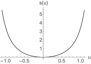
Figure 1: The curve s vs $u$ for $a=1$ for the hyperbola parametrized by circular functions.

II.2 NLD equation constrained to an ellipse

For the other conical sections the formalism is the same, just the parametric representation is changed. Since the spin connection is zero for these transformations, one can obtain the transformation to the 1+1 dimensional Dirac equation directly from the metric. For the ellipse centered at the coordinate origin

$$x=a\cos\theta\,,~{}~{}~{}y=b\sin\theta\,,$$ (10)

so that

$$ds^{2}=-dt^{2}+dx^{2}+dy^{2}=-dt^{2}+(a^{2}\sin^{2}\theta+b^{2}\cos^{2}\theta)d\theta^{2}\,.$$ (11)

We see that we can reduce the metric to a $1+1$ dimensional Minkowski form by the transformation:

$$d\textbf{s}=\sqrt{a^{2}\sin^{2}\theta+b^{2}\cos^{2}\theta}~{}d\theta\,.$$ (12)

Explicitly

$$\textbf{s}[\theta]=bE\left(\theta\left|1-\frac{a^{2}}{b^{2}}\right.\right)\,,$$ (13)

where $E(x,m)$ is the incomplete elliptic integral of the second kind with modulus $m$ AS . When $a=1,b=2$ we get the transformation shown in Fig. 2. For a circle ($a=b$) the above equation reduces to $s(\theta)=a\theta$.

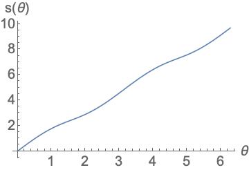
Figure 2: The arc variable curve s vs $\theta$ for $a=1,~{}~{}b=2$ for the ellipse.

II.3 NLD equation constrained to a parabola

For the parabola $x^{2}=4ay$, the parametric equations are

$$x=2a\eta\,,~{}~{}~{}y=a\eta^{2}\,.$$ (14)

Then

$$ds^{2}=-dt^{2}+dx^{2}+dy^{2}=-dt^{2}+4a^{2}(1+\eta^{2})d\eta^{2}\,.$$ (15)

Here changing variables to

$$d\textbf{s}=2a~{}\int\sqrt{1+\eta^{2}}~{}d\eta$$ (16)

brings the metric back into the Minkowski form. Explicitly

$$\textbf{s}[\eta]=a\left(\eta~{}\sqrt{\eta^{2}+1}+\sinh^{-1}(\eta)\right)\,.$$ (17)

When $a=1$ we obtain the curve shown in Fig. 3.

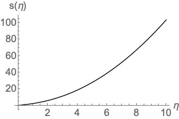
Figure 3: The arc variable curve s vs $\eta$ for $a=1$ for the parabola.

III Normalized Charge Density

What we have shown for the NLD equation in $2+1$ dimensions constrained to the three conic sections, that we can reduce the $2+1$ dimensional NLDE to the flat space $1+1$ dimensional NLDE if we use the arc length variable. The static solutions of the NLDE in 1+1 dimensions can be written in the form:

$$\psi(x) =\left(\begin{array}[]{cc}u(x)\\ i~{}v(x)\\ \end{array}\right)=R(x)\left(\begin{array}[]{c}\cos\theta\\ i\sin\theta\end{array}\right),$$ (22)

where

$$u^{2} =R^{2}\cos^{2}\theta=\frac{2}{g^{2}}\frac{(m^{2}-\omega^{2})(m+\omega)\cosh^{2}\beta x}{(m+\omega\cosh 2\beta x)^{2}},$$

$$v^{2} =R^{2}\sin^{2}\theta=\frac{2}{g^{2}}\frac{(m^{2}-\omega^{2})(m-\omega)\sinh^{2}\beta x}{(m+\omega\cosh 2\beta x)^{2}},$$ (23)

as discussed in ref:numerical and more recently for arbitrary nonlinearity in NLD . As a function of $\omega/m$ the shape of the solitary wave changes from single humped to double humped as one lowers $\omega/m$. As a function of the arc length s the density of the solitary wave is given by $\rho(\textbf{s})=R^{2}(\textbf{s})$

$$\rho(\textbf{s})=\Psi^{{\dagger}}\Psi=\frac{2\beta^{2}}{g^{2}(m+\omega)}\frac{1+\alpha^{2}\tanh^{2}\beta\textbf{s}}{(1-\alpha^{2}\tanh^{2}\beta\textbf{s})^{2}}{\rm sech}^{2}\beta\textbf{s}\,.$$ (24)

Here (with frequency $\omega$)

$$\beta=\sqrt{m^{2}-\omega^{2}}\,,~{}~{}~{}\alpha^{2}=\frac{m-\omega}{m+\omega}\,,$$ (25)

and the total charge is

$$Q=\int d\textbf{s}\Psi^{{\dagger}}\Psi=\frac{2\beta}{g^{2}\omega}\,.$$ (26)

In Fig. 4 we plot $\rho/Q[\omega]$ vs. $s$ for two values, $\omega=0.9$ which is single humped and $\omega=1/4$ which is double humped.

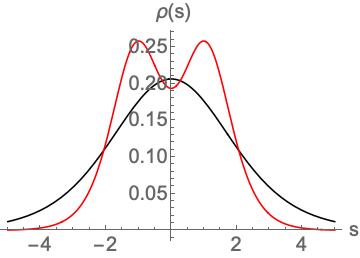
Figure 4: Normalized charge density vs. the arc length $s$ for $\omega=0.9$ (black) and $\omega=1/4$ (red) for NLD on a straight line.

III.1 Hyperbola

We now wish to discuss the change in shape of the solitary wave as we go from the arc variable s to the parametric representation of the curve variable $u$ when the two dimensional motion is confined to a hyperbola. The arc length in terms of $u$ is given by

$$\textbf{s}[a,u]=a(\sec(u)\sqrt{\tan^{2}(u)+\sec^{2}(u)}-1)\,.$$ (27)

In what follows we will always choose the mass $m=1$ , and take $g=1$. Later on we will use the symbol $m$ to describe the modulus of Jacobi elliptic functions. This is not to be confused with the Dirac mass $m$ which we set to one. In Fig. 5 we plot $\rho/Q[\omega]$ vs. $u$ for the same two values $\omega=0.9$ which is single humped and $\omega=1/4$ which is double humped. We see that the solitary wave shape is quite different (i.e. contracted, see the horizontal axis) when the solitary wave is plotted vs. $u$

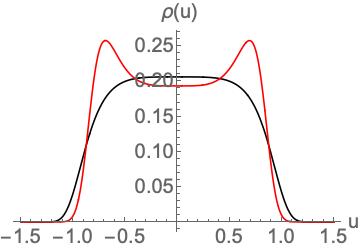
Figure 5: Normalized charge density for a soliton constrained to a hyperbola vs. $u$ for $,\omega=0.9$ (black) and $\omega=1/4$ (red).

III.2 Ellipse

Choosing for the parameters of the ellipse $a=1,b=2$, we have that the arc length is given by

$$s[\theta]=2E\left(\theta\left|\frac{3}{4}\right.\right)\,.$$ (28)

The curve for the normalized charge densities for the curve constrained to the ellipse with $b=2,a=1$ is shown in Fig. 6 and is contracted.

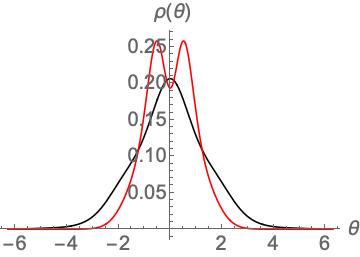
Figure 6: Normalized charge density for a soliton constrained to an ellipse with $a=1,b=2$ vs. $\theta$ for $\omega=0.9$ (black) and $\omega=1/4$ (red).

III.3 Parabola

Choosing for the parameters of the parabola $a=1$, we have that the arc length is given by

$$\textbf{s}[\eta]=\eta\sqrt{\eta^{2}+1}+\sinh^{-1}(\eta)\,.$$ (29)

The curve for the normalized charge densities for the curve constrained to a parabola is shown in Fig. 7. It is even more contracted.

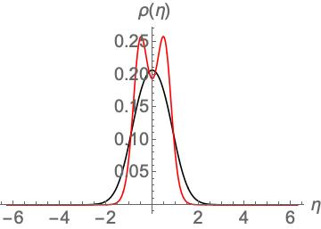
Figure 7: Normalized charge density for the soliton constrained to a parabola vs. $\eta$ for $\omega=0.9$ (black) and $\omega=1/4$ (red).

IV Other parameterizations of the conic sections

Of course there are other parameterizations of the conic sections which give different expressions for the arc length in terms of these parameters. For example, we can parametrize the ellipse, using doubly periodic functions–namely the Jacobi elliptic functions and we can parametrize the hyperbola and the parabola using hyperbolic functions.

IV.1 Jacobi elliptic parametrization of the ellipse

In the simplest case we can let

$$x=a\text{cn}(\theta,m)\,,~{}~{}~{}y=b\text{sn}(\theta,m)\,,$$ (30)

when the modulus $m\rightarrow 0$ the Jacobi elliptic functions $\text{cn}(x,k)$ and $\text{sn}(x,k)$ AS become the circular functions $\cos(u)$ and $\sin(u)$, respectively. The spatial part of the metric is

$$dx^{2}+dy^{2}=\text{dn}(\theta|m)^{2}\left(a^{2}\text{sn}(\theta|m)^{2}+b^{2}\text{cn}(\theta|m)^{2}\right)(d\theta)^{2}\,,$$ (31)

so that the change of variables is:

$$d\textbf{s}=\text{dn}(\theta|m)\sqrt{a^{2}\text{sn}(\theta|m)^{2}+b^{2}\text{cn}(\theta|m)^{2}}d\theta\,.$$ (32)

Integrating we get:

$$\textbf{s}=bE\left(\text{am}(\theta|m)\left|1-\frac{a^{2}}{b^{2}}\right.\right)\theta\,,$$ (33)

which simplifies to our previous result when $b=2a$. Here ${\rm am}(\theta,m)$ is the Jacobi amplitude function AS . The Jacobi ellipse is shown, with $a=3$, $b=5$, $m=1/3$ in Fig. 8.

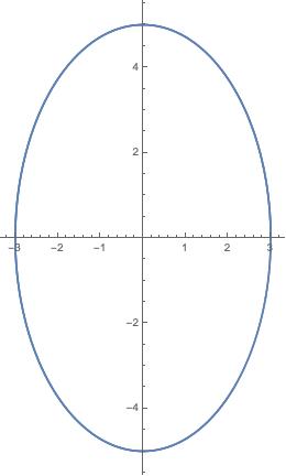
Figure 8: The Jacobi elliptic curve $\{x[\theta],y[\theta]\}$ for $a=3,b=5,m=1/3$ .

For the densities parametrized as a function of $\theta$ of the Jacobi elliptic function we find the results shown in Fig. 9

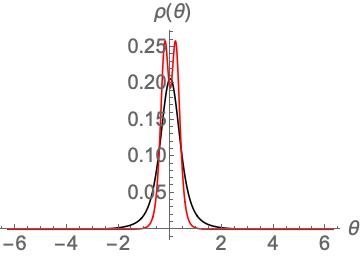
Figure 9: Normalized charge density for the soliton constrained to an ellipse vs. $\theta$ for $\omega=0.9$ (black) and $\omega=1/4$ (red) for the Jacobi elliptic function parametrization with $b=5,a=3,m=1/3$. It is contracted compared to Fig. 6.

IV.2 A different hyperbolic function parametrization of the hyperbola

Let us consider the following parametrization of the hyperbola in terms of hyperbolic functions

$$x=a\sinh(\theta)\,,~{}~{}y=a\cosh(\theta)\,.$$ (34)

For this alternative parametrization of the hyperbola we find

$$ds^{2}=a^{2}\cosh(2\theta)d\theta^{2}\,,$$ (35)

and

$$s=-iaE(iu|2)\,.$$ (36)

In terms of this parameterization we get the densities shown in Fig. 10 when we choose $a=2$.

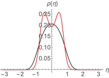
Figure 10: Normalized charge density for the soliton constrained to a hyperbola vs. $\theta$ for $\omega=0.9$ (black) and $\omega=1/4$ (red) for the hyperbolic function parametrization with $a=2$.

IV.3 Hyperbolic function parametrization of a parabola

Instead of the parametrization given above of the parabola we could have used a parametrization in terms of hyperbolic functions:

$$x=2a\sinh(\eta)\,,~{}~{}y=a\sinh^{2}(\eta)\,,$$ (37)

so that again $x^{2}=4ay$. Note that for small $\eta$ this parametrization goes over to the parametrization used earlier. The spatial part of the metric then becomes

$$dx^{2}+dy^{2}=4a^{2}\cosh^{4}(\eta)~{}d\eta^{2}\,.$$ (38)

Thus the appropriate change of variables to a $1+1$ dimensional metric is captured in

$$ds=2a\cosh^{2}(\eta)d\eta\,.$$ (39)

In this way, we obtain

$$s(\eta)=a[\eta+\sinh(2\eta)/2]\,.$$ (40)

One obtains for the normalized densities in the two cases studied before the results shown in Fig. 11.

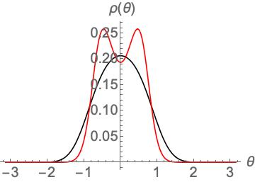
Figure 11: Normalized charge density for the soliton constrained to a parabola vs. $\eta$ for $,\omega=0.9$ (black) and $\omega=1/4$ (red) for the hyperbolic function parametrization with $a=1$.

V Solitary wave solutions for the $3+1$ dimensional NLDE confined to a space curve

V.1 Helix

The helix is a space curve with parametric equations:

$$x=r\cos\theta\,,~{}~{}~{}y=r\sin\theta\,,~{}~{}~{}z=c\theta\,.$$ (41)

Here $r$ is the radius of the helix and $2\pi c$ gives the vertical separation of the helix’s hoops, i.e. pitch. The curvature of the helix $\kappa$ is given by

$$\kappa=\frac{r}{r^{2}+c^{2}}\,,$$ (42)

which is constant and the torsion $\tau$ is given by

$$\tau=\frac{c}{r^{2}+c^{2}}\,,$$ (43)

which is also constant. For this problem we find the metric is given by

$$ds^{2}=-d\tau^{2}+dx^{2}+dy^{2}+dz^{2}=-d\tau^{2}+(r^{2}+c^{2})d\theta^{2}\,.$$ (44)

Therefore, for this problem, the simple transformation to the 1+1 Minkowski metric is again in terms of the arc length

$$d\textbf{s}=\sqrt{r^{2}+c^{2}}d\theta\,.$$ (45)

So again in the $1+1$ dimensional space the transformation is given by

$$d\textbf{s}=\sqrt{-g}d\theta\,.$$ (46)

V.2 Elliptic helix

The elliptic helix, i.e. a helix with an elliptic cross-section on projection, is defined by

$$x=a\cos\theta\,,~{}~{}~{}y=b\sin\theta\,,~{}~{}~{}z=k\int\sqrt{a^{2}\sin^{2}\theta+b^{2}\cos^{2}\theta}d\theta\,.$$ (47)

Note that $dz^{2}$ = $k^{2}(dx^{2}+dy^{2})$ so that the 3D arc length is proportional to the 2D arc length. The curvature is variable in this case. Performing the integral we get

$$z=aE\left(\theta\left|1-\frac{b^{2}}{a^{2}}\right.\right)\,.$$ (48)

The metric is given by

$$ds^{2}=-d\tau^{2}+dx^{2}+dy^{2}+dz^{2}=-d\tau^{2}+(1+k^{2})(a^{2}\cos^{2}(\theta)+b^{2}\sin^{2}(\theta))d\theta^{2}\,,$$ (49)

so that again one can transform this to a Minkowski metric with the transformation utilizing the arc length

$$d\textbf{s}=\sqrt{-g}d\theta=\sqrt{1+k^{2}}\sqrt{a^{2}\cos^{2}(\theta)+b^{2}\sin^{2}(\theta)}~{}d\theta\,.$$ (50)

Thus, the explicit transformation is (for $a>b>0$)

$$\textbf{s}=\sqrt{1+k^{2}}aE\left(\theta\left|1-\frac{b^{2}}{a^{2}}\right.\right)\,.$$ (51)

V.3 Jacobi elliptic helix

The Jacobi elliptic helix can be parametrized as follows:

$$x=a\text{cn}(\theta~{}|m)\,,~{}~{}~{}y=b\text{sn}(\theta~{}|m)\,,~{}~{}~{}z=k\int d\theta~{}\text{dn}(\theta|m)\sqrt{\left(a^{2}\text{sn}(\theta|m)^{2}+b^{2}\text{cn}(\theta|m)^{2}\right)}\,.$$ (52)

Performing the integral we have

$$z=kbE\left(\text{am}(\theta|m)\left|1-\frac{a^{2}}{b^{2}}\right.\right)\,.$$ (53)

The space curve is shown in Fig. 12, and

$$dx^{2}+dy^{2}+dz^{2}=(1+k^{2})(\text{dn}(\theta|m))^{2}\left(a^{2}\text{sn}(\theta|m)^{2}+b^{2}\text{cn}(\theta|m)^{2}\right)\,.$$ (54)

So we see that we can transform this to a 1D Dirac equation by letting

$$d\textbf{s}=\sqrt{1+k^{2}}\text{dn}(\theta|m)\sqrt{\left(a^{2}\text{sn}(\theta|m)^{2}+b^{2}\text{cn}(\theta|m)^{2}\right)}d\theta\,.$$ (55)

Integrating, we get the arc variable

$$\textbf{s}=\sqrt{1+k^{2}}bE\left(\text{am}(\theta|m)\left|1-\frac{a^{2}}{b^{2}}\right.\right)\,.$$ (56)

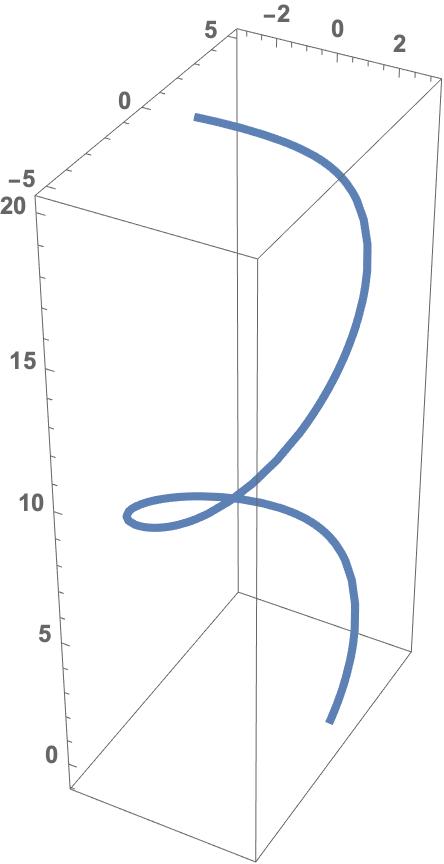
Figure 12: The Jacobi elliptic helix curve $\{x[\theta],y[\theta],z[\theta]\}$ for $a=3,b=5,m=1/3,k=1$.

V.4 Helix of the hyperboloid of revolution

The hyperboloid of revolution is defined by

$$\frac{x^{2}+y^{2}}{a^{2}}-\frac{z^{2}}{b^{2}}=1.$$ (57)

The helix of the one-sheeted hyperboloid of revolution can be parametrized as follows:

$$x=a\cosh\eta\cos{f(\eta)}\,,~{}~{}~{}y=a\cosh\eta\sin{f(\eta)}\,,~{}~{}~{}z=b\sinh\eta\,,$$ (58)

where

$$\frac{df}{d\eta}=\sqrt{\left(\frac{b}{a\tan\alpha}\right)^{2}-\tanh^{2}\eta}\,.$$ (59)

The curve $f[\eta]$ depends on whether

$$\beta=\frac{b}{a\tan\alpha}$$ (60)

is less than one or greater than or equal to one. In the latter case $f[\eta]$ is a straight line. In our plot, Fig. 13, we consider the cases $\beta=1/2,1,10$ to exemplify the possibilities.

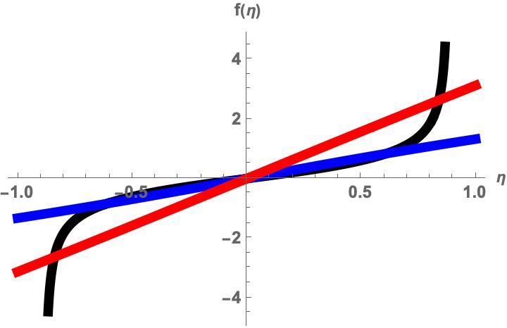
Figure 13: The curves $f[\eta]$ for $\beta=1/2,1,10$, drawn in black, blue and red. Here we have chosen $a=1$, $b=1/2$.

Explicitly,

$$f_{1/2}(\eta) =\frac{\cosh(\eta)\left(\sqrt{6-2\cosh(2\eta)}\sin^{-1}(\sinh(\eta))-2\sqrt{\cosh(2\eta)-3}\tanh^{-1}\left(\frac{2\sinh(\eta)}{\sqrt{\cosh(2\eta)-3}}\right)\right)}{\cosh(2\eta)-3}\,,$$

$$f_{1}(\eta) =\frac{\cosh(\eta)\sqrt{4-2\tanh^{2}(\eta)}\left(\sinh^{-1}\left(\frac{\sinh(\eta)}{\sqrt{2}}\right)+\tan^{-1}\left(\frac{\sqrt{2}\sinh(\eta)}{\sqrt{\cosh(2\eta)+3}}\right)\right)}{\sqrt{\cosh(2\eta)+3}}\,,$$

$$f_{10}(\eta) =\frac{\cosh(\eta)\sqrt{20-2\tanh^{2}(\eta)}\left(3\sinh^{-1}\left(\frac{3\sinh(\eta)}{\sqrt{10}}\right)+\tan^{-1}\left(\frac{\sqrt{2}\sinh(\eta)}{\sqrt{9\cosh(2\eta)+11}}\right)\right)}{\sqrt{9\cosh(2\eta)+11}}\,.$$ (61)

From Eq. (58) one can show that the differential arc length is

$$d\textbf{s}=b\csc(\alpha)\cosh(\eta)\,.$$ (62)

Since

$$dz=b\cosh(\eta)\,,$$ (63)

therefore the parameter $\alpha$ has the meaning

$$\frac{dz}{d\textbf{s}}=\sin\alpha$$ (64)

and the arc length is given by

$$\textbf{s}=b\csc(\alpha)\sinh(\eta)\,.$$ (65)

The helices for $\beta=1/2,1,10$ are shown in Fig. 14.

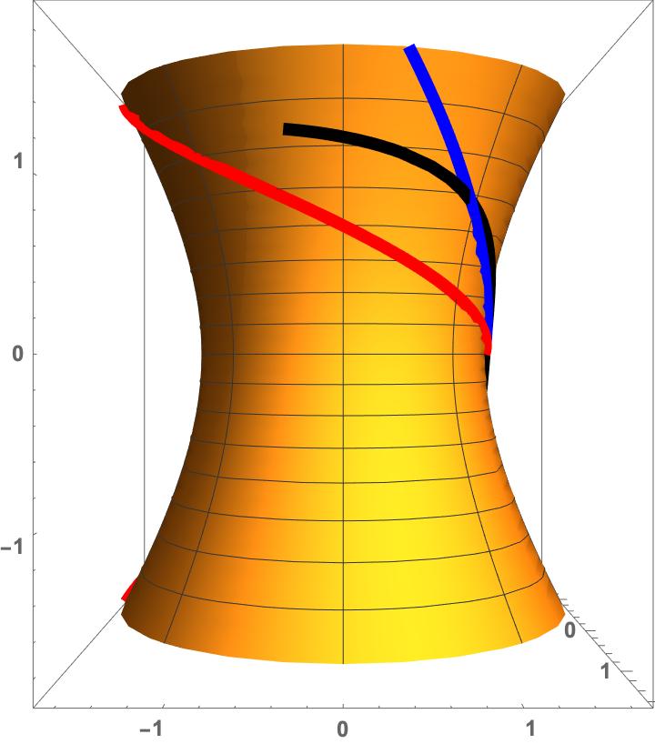
Figure 14: The helices for $\beta=1/2,1,10$, are drawn in black, blue and red on a one-sheeted hyperboloid of revlution. Here we have chosen $a=1$, $b=1/2$.

VI Conclusions

We have studied the behavior of the nonlinear Dirac equation ref:numerical ; NLD on planar and space curves. We have shown here how the arc length variable is the relevant choice to study the nonlinear Dirac equation on planar and space curves. We studied different parameterizations of various curves including those involving Jacobi elliptic functions AS and studied the charge density in the presence of a soliton. We found the change in soliton shape in terms of narrowing or broadening of the soliton profile in the curved region. These results illustrate an insightful interplay between solitons of the nonlinear Dirac equation and the curvature (and torsion) of a variety of curves. Our results are relevant to curved Q1D Bose condensates assuming they can be realized experimentally. It would be instructive to (numerically) study collisions of NLD solitons on various curves to explore how curvature (and torsion) affect their interaction and collision dynamics including bounce windows.

VII Acknowledgment

A.K. is grateful to Indian National Science Academy (INSA) for the award of INSA Senior Scientist position at Savitribai Phule Pune University. This work was supported in part by the U.S. Department of Energy.

VIII Appendix: The viebein formalism applied to a hyperbola

The vierbein introduced by Hermann Weyl Weyl is also called a tetrad or a frame field (in general relativity). We shall use the metric convention $(-++)$ for the $2+1$ space-time which is commonly used in the curved-space literature. In what follows, we use Greek indices for the curvilinear coordinates $\eta$ or $\theta$, and Latin indices for the Minkowski coordinates $x,y$ and $t$. To obtain the fermion evolution equations in the new coordinate system it is simplest to use a coordinate covariant action such as that used in field theory in curved spaces, even though here the actual curvature is zero. For the constrained system, the $2+1$ dimensional Minkowski line element

$$(ds)^{2} =-(dt)^{2}+(dx)^{2}+(dy)^{2}$$ (66)

$$=-(dt)^{2}+a^{2}\cosh 2\eta(d\eta)^{2}\equiv-(dt)^{2}+(d\textbf{s})^{2}\,,$$

so that the original Minkowski metric

$$g_{\alpha\beta}={\rm diag}\{-1,1,1\}$$ (67)

reduces to an effective curved space $1+1$ dimensional metric tensor:

$$g_{\mu\nu}={\rm diag}\{-1,a^{2}\cosh 2\eta\}$$ (68)

with inverse

$$g^{\mu\nu}={\rm diag}\{-1,\frac{1}{a^{2}\cosh 2\eta}\}.$$ (69)

Vierbeins transform the curved 1+1 dimensional space to a locally Minkowski 1+1 dimensional space via. $g_{\mu\nu}=V^{a}_{\mu}V^{b}_{\nu}\eta_{ab},$ where $\eta_{ab}=(-1,1)$ is the flat Minkowski metric. A convenient choice for the vierbein is

$$V_{\mu}^{a}={\rm diag}\{1,a\sqrt{\cosh 2\eta}\}~{},$$ (70)

so that

$$V^{\mu}_{a}={\rm diag}\left\{1,\frac{1}{a\sqrt{\cosh 2\eta}}\right\}\,.$$ (71)

The determinant of the metric tensor is given by

$$\det V=\sqrt{-g}=a\sqrt{\cosh 2\eta}\,.$$ (72)

The action for our model in general curvilinear coordinates is

$$S[\Psi,\sigma]=\int d^{3}x~{}\det V\bigg{(}{-i\over 2}\bar{\Psi}\tilde{\gamma}^{\mu}\nabla_{\mu}\Psi+{i\over 2}(\nabla_{\mu}^{\dagger}\bar{\Psi})\tilde{\gamma}^{\mu}\Psi-i(m\bar{\Psi}\Psi)-\frac{g^{2}}{2}(\bar{\Psi}\Psi)^{2}\bigg{)}\,.$$ (73)

The coordinate dependent gamma matrices $\tilde{\gamma}^{\mu}$ are obtained from the usual Dirac gamma matrices $\gamma^{a}$ via

$$\tilde{\gamma}^{\mu}=\gamma^{a}V_{a}^{\mu}(x)\ .$$ (74)

The coordinate independent Dirac matrices $\gamma^{a}$ satisfy the usual gamma matrix algebra:

$$\{\gamma^{a},\gamma^{b}\}=2\eta^{ab}~{}.$$ (75)

From the action Eq. (73) we obtain the Heisenberg field equation for the fermions,

$$\left(\tilde{\gamma}^{\mu}\nabla_{\mu}+\sigma+m\right)\Psi=0\,,$$ (76)

where it is to be understood:

$$\sigma=-ig^{2}\bar{\Psi}\Psi\,.$$ (77)

This can be generalized easily to the case where the nonlinear term in the NLDE is of the form NLD

$$-g^{2}(\bar{\Psi}\Psi)^{\kappa}\Psi\,,$$ (78)

with $\kappa$ denoting arbitrary nonlinearity. This is done by letting

$$\sigma=-ig^{2}(\bar{\Psi}\Psi)^{\kappa}$$ (79)

in the equation of motion. This again is space and time dependent mass, but a scalar as we will show below.

Here $\tilde{\gamma}^{\mu}=\gamma^{a}V_{a}^{\mu}$, $\nabla_{\mu}=\partial_{\mu}+\Gamma_{\mu}$, and $\Gamma_{\mu}$ is the spin connection given by Birrell_Davies ; Weinberg

$$\Gamma_{\mu}={1\over 2}\Sigma^{ab}V_{a\nu}(\partial_{\mu}V_{b}^{\nu}+\Gamma^{\nu}_{\mu\lambda}V_{b}^{\lambda})\,,~{}~{}~{}\Sigma^{ab}={1\over 4}[\gamma^{a},\gamma^{b}].$$ (80)

We have

$$\tilde{\gamma}^{0}=\gamma^{0};~{}~{}\tilde{\gamma}^{1}=\frac{1}{a\sqrt{\cosh 2\eta}}\gamma^{1}\,.$$ (81)

We will choose for convenience the following representation for the matrices $\gamma^{0}$ and $\gamma^{1}$ in the transformed local Minkowski 1+1 dimensional Dirac equation.

$$i\gamma^{0}=\left(\matrix{1&0\cr 0&-1\cr}\right)\,,$$ (82)

$$\gamma^{1}=\left(\matrix{0&1\cr 1&0\cr}\right)\,.$$

We have that the scalar field $\sigma$ is unchanged in form

$$\sigma=-ig^{2}(\Psi^{\dagger}\tilde{\gamma}^{0}\ \Psi)=-ig^{2}(\Psi^{\dagger}{\gamma}^{0}\ \Psi)\,,$$ (83)

if we used Eq. (79) to define $\sigma$, it would again be unchanged in form.

The Christoffel symbols have the usual definition, $\Gamma^{\sigma}_{\mu\lambda}=\frac{1}{2}g^{\nu\sigma}(\partial_{\lambda}g_{\nu\mu}+\partial_{\mu}g_{\nu\lambda}-\partial_{\nu}g_{\mu\lambda})$. Since the only non-zero derivative is

$$\frac{\partial g_{22}}{\partial x^{2}}=2a^{2}\sinh 2\eta,$$ (84)

we find the only nonzero Christoffel symbol is

$$\Gamma_{222}=a^{2}\sinh 2\eta$$ (85)

so that

$$\Gamma^{2}_{22}=\tanh 2\eta\,.$$ (86)

We find the spin connection is zero for the following reason. If we consider

$$F_{\mu,b}^{\nu}=\partial_{\mu}V_{b}^{\nu}+\Gamma^{\nu}_{\mu\lambda}V_{b}^{\lambda}\,,$$ (87)

only $F_{22}^{2}$ could have a non-zero contribution but we find

$$\partial_{\nu}V_{2}^{2}=-\frac{\tanh 2\eta}{a\sqrt{\cosh 2\eta}};~{}~{}\Gamma_{2}^{22}V_{2}^{2}=+\frac{\tanh 2\eta}{a\sqrt{\cosh 2\eta}}\,,$$ (88)

so that $F_{22}^{2}=0$ which implies that the spin connection is zero.

From Eq. (76), and the fact that the spin connection is zero we find that the equation of motion for $\Psi$ is

$$(\tilde{\gamma}^{\mu}\partial_{\mu}+\sigma+m)\Psi=0.$$ (89)

Writing this out more explicitly, we obtain

$$\left(\gamma^{0}\partial_{t}+\frac{1}{a\sqrt{\cosh 2\eta}}\gamma^{1}\partial_{\eta}+\sigma+m\right)\Psi[\eta,t]=0.$$ (90)

References

- (1) See e.g., L. H. Haddad and L. D. Carr, New J. Phys. 17, 113011 (2015).
- (2) H. Weyl, Zeitschrift Physik 56, 330 (1929).
- (3) Y. B. Gaididei, S. F. Mingaleev, and P. Christiansen, Phys. Rev. E 62, R53 (2000).
- (4) M. Ibanes, J. M. Sancho, and G. P. Tsironis, Phys. Rev. E 65, 041902 (2002).
- (5) A. Ludu, Nonlinear Waves and Solitons on Contours and Closed Surfaces (Springer Series in Synergetics, Second edition, Berlin 2012).
- (6) D. J. Gross and A. Neveu, Phys. Rev. D10, 3235 (1974).
- (7) A. Chodos, F. Cooper, W. Mao, and A. Singh Phys. Rev. D 63 096010 (2001); hep-ph/0011211.
- (8) M. Abamowitz and I. A. Stegun, Eds. Handbook of Mathematical Functions (Dover Publications, Mineola, New York, 1965).
- (9) A. Alvarez and B. Carreras, Phys. Lett. 86A, 327, (1981).
- (10) F. Cooper, A. Khare, B. Mihaila, and A. Saxena, Phys. Rev. E 82, 036604 (2010).
- (11) N. D. Birrell and P. C. W. Davies Quantum Fields in Curved Space (Cambridge University Press, Cambridge, 1982).
- (12) S. Weinberg, Gravitation and Cosmology: Principles and Applications of the General Theory of Relativity (Wiley, New York, 1972).