Time fractional stochastic differential equation with random jumps

Abstract.

We prove the well-posedness of variable-order time fractional stochastic differential equations with jumps. Using a truncating argument, we do not assume any condition on the initial distribution and the integrability of the large jump term even though the solution is non-Markovian. To get moment estimates, some extra assumptions are needed. As an application of moment estimates, we prove the Hölder regularity of the solutions.

Keywords: variable-order time fractional stochastic differential equation, stochastic Volterra equation, Lévy noise, well-posedness, moment estimates, regularity.

1. Introduction

1.1. Background and outline of the paper

Stochastic differential equations (abbreviated as SDE) are used to describe phenomena such as particle movements with a random forcing, often modeled by Brownian motion noise (continuous)[13, 18, 26] or Lévy noise (jump type) [2, 30].
The classical Langevin equation describes the random motion of a particle immersed in a liquid due to the interaction with the surrounding liquid molecules. Let $m$ be the mass of the particle, and $x(t)$ and $u(t)$ be the instantaneous position and velocity of the particle. Then Newton’s equation of motion for the Brownian particle is given by the Langevin equation

$$m\frac{du}{dt}=-\gamma u+\xi(t).$$ (1)

Here $\gamma$ is the friction coefficient per unit mass, and $\xi(t)$ is the random force that accounts for the effect of background noise and is usually described by a white noise, i.e., the correlation function satisfies

$$\langle\xi(t)\rangle=0,\ \langle\xi(t_{1}),\xi(t_{2})\rangle=2D\delta(t_{1}-t_{2}).$$

It is well known that (1) is equivalent to the following SDE:

$$du=-\frac{\gamma}{m}u(t)dt+\frac{1}{m}dW_{t}.$$ (2)

where $W_{t}$ is Brownian motion, and which generalizes to the general SDE:

$$du=f(t,u(t))dt+g(t,u(t))dW_{t}.$$ (3)

However, when the particle is immersed in viscoelastic liquids, the temporal moments of the random force has memory effect and is often a power function of time $t$

$$\langle\eta(t)\rangle=0,\ \langle\eta(0),\eta(t)\rangle=\Gamma(\alpha)t^{-\alpha},$$

leading to the generalized Langevin equation [19]

$$\frac{du}{dt}+\int_{0}^{t}K(t-s)u(s)ds=\eta(t)$$ (4)

with $K$ being the kernel, which is equivalent to the following stochastic Volterra equation driven by fractional Brownian motion:

$$du=\int_{0}^{t}\kappa(t,s)u(s)ds+dW^{H}(t)$$ (5)

where $W^{H}(t)$ is a fractional Brownian motion with Hurst index $H$. We refer the reader to [17] for the modeling, and [9] for the well-posedness of (5).

Different fractional Langevin equations were derived via the Laplace transform based on the generalized Langevin equation (4). For example, in [7, 22], the fractional Langevin equation of the form

$$\frac{du}{dt}+\gamma D_{t}^{\alpha}u=\eta(t),\quad 0<\alpha<1.$$ (6)

was derived. In [33], they similarly derived a fractional Langevin equation that assumes different forms at different time scales. Namely,

$$\frac{du}{dt}+u=\eta(t),~{}~{}0<t\ll\tau\qquad\frac{du}{dt}+\gamma D_{t}^{1/2}u=\eta(t),~{}~{}t\gg\tau$$ (7)

where $\tau$ is the mean collision time of the liquid molecules with the particle.
Moreover, the surrounding medium of the particle may change with time, which leads to the change of the fractional dimension of the media that in turns leads to the change of the order of the fractional Langevin equation via the Hurst index [11, 23] and yields a variable-order fractional Langevin equation of the form

$$du=-\gamma D_{t}^{\alpha(t)}udt+dW^{H}(t)$$ (8)

All of the above examples focus on fractional Langevin equation with (fractional) Brownian noise. However, when the surrounding medium of the particle exhibits strong heterogeneity, the particle may experience large jumps and lead to an additional Lévy driven noise [3]. In this paper, we will focus on pure jump noise. Our model can be expressed as the following variable-order time fractional SDE driven by a multiplicative Lévy noise which also includes a large jump term:

$$du(t) =\big{(}\lambda\cdot{}_{0}^{R}D_{t}^{\alpha(t)}u(t)+f(t,u(t))\big{)}dt+\int_{|z|<1}g\big{(}t,u(t-),z\big{)}\widetilde{N}(dt,dz)$$ (9)

$$\quad+\int_{|z|\geq 1}h\big{(}t,u(t-),z\big{)}N(dt,dz),u(0)=u_{0},\qquad t\in[0,T],$$

where $T>0,\lambda\in\mathbb{R}$, ${}_{0}^{R}D_{t}^{\alpha(t)}u(t)$ represents friction with memory effect, $f(t,u(t))$ is the external force and the random terms represent the jump type noise. Here the variable-order Riemann-Liouville derivative is given by

$$_{0}^{R}D_{t}^{\alpha(t)}u(t):=\frac{d}{dt}\int_{0}^{t}\frac{u(s)}{\Gamma(1-\alpha(t))(t-s)^{\alpha(t)}}ds,$$ (10)

where $\alpha,f,g,h$ are functions in proper classes which make the integrals meaningful. One can see similar definitions of fractional derivatives from [14, 15, 23, 24, 28, 32, 35, 39].
As we will see in (12), our equation can be seen as a special form of stochastic Volterra equation, with no memory effect on the random noise. For the properties of general stochastic Volterra equation, with memory effect on the random noise, we refer the reader to [6, 27, 38] for white noise driven stochastic Volterra equation and [1, 4, 8, 12, 29] for Lévy driven noise.
The reason why we do not consider memory effect on the random noise is that it can be treated similarly once we apply the moment inequalities, see Lemma 3.7. Also, the memory effect on the drift term already makes the equation essentially different from the usual SDE because the solution will be non-Markovian. Therefore, it is not easy to argue that the equation has a unique solution with any initial distribution which is used to add the large jump noise.
In our paper, we aim to prove that our equation has a unique solution with any initial distribution, even though we do not have Markov property. Using this fact, with extra analysis, we show that without any condition on the large jump term, existence and uniqueness of (9) holds. According to the authors’ knowledge, this is the first time showing that fact in non-Markovian setting.
Moreover, since the kernel function is given by fractional derivative, which is special in that it has some scaling properties, we discover that the decaying speed in the approximating procedure of the solution is slower than the usual SDE, and it can be given explicitly by the fractional order of the derivative, see Theorem 2.2. Also, the explicit relation between the regularity of the solution and the regularity of the fractional order is also derived, see Theorem 2.5.

Outline of the paper: The rest of this paper is organized as follows: In the remaining of Section 1, we will talk about an illustrative example. Also, some preliminaries and notations will be mentioned. In Section 2, we will formulate the assumptions and main theorems. In Section 3, we prove the well-posedness of (9). Indeed, we will prove a stronger result Proposition 3.9 which implies the well-posedness. In Section 4, we prove the moment estimates of the solution and as an application, we prove the Hölder regularity of the solution. In Section 5, we discuss some further questions, including some questions which are interesting but are outside the scope of this paper.

1.2. An illustrative example

Before we formulate our main problem, we consider the following illustrative example.

$$du(t)=\big{(}\lambda\cdot{}_{0}^{R}D_{0}^{\alpha(t)}u(t)+f(t,u(t))\big{)}dt+h(t,u(t-))\delta_{t_{0}}(t),t\in[0,T],u(0)=u_{0}\in\mathbb{R},$$

where $t_{0}\in(0,T)$ is a fixed time and $\delta_{t_{0}}$ is the Dirac measure supported at $\{t_{0}\}$. Then the above equation can be understood as the following Volterra equation with a jump at time $t_{0}$:

$$u(t)=u_{0}+\lambda\int_{0}^{t}\frac{u(s)}{\Gamma(1-\alpha(t))(t-s)^{\alpha(t)}}ds+\int_{0}^{t}f(s,u(s))ds+\int_{0}^{t}h(s,u(s-))\delta_{t_{0}}(ds).$$

Due to the memory of the term ${}_{0}^{R}D_{t}^{\alpha(t)}u(t)$, solving the above deterministic equation is not as easy as the memoryless case. The reason is that after the jump, the solution not only depends on the behavior at the jump time, but also depends on the past. Thus we need a finer piecewise analysis as below:
If $t<t_{0}$, the equation reduces to the Volterra equation with no jump:

$$u(t)=u_{0}+\lambda\int_{0}^{t}\frac{u(s)}{\Gamma(1-\alpha(t))(t-s)^{\alpha(t)}}ds+\int_{0}^{t}f(s,u(s))ds,$$

and the solution is denoted as $v_{0}(t),t<t_{0}$.
If $t=t_{0}$, the solution is given by

$$u(t_{0})=u_{0}+\lambda\int_{0}^{t_{0}}\frac{v_{0}(s)}{\Gamma(1-\alpha(t))(t_{0}-s)^{\alpha(t_{0})}}ds+\int_{0}^{t_{0}}f(s,v_{0}(s))ds+h(t_{0},v_{0}(t_{0}-)),$$

If $t>t_{0}$, the solution is given by the following equation

$$u(t) =u_{0}+\lambda\int_{0}^{t_{0}}\frac{v_{0}(s)}{\Gamma(1-\alpha(t))(t-s)^{\alpha(t)}}ds+\int_{0}^{t_{0}}f(s,v_{0}(s))ds+h(t_{0},v_{0}(t_{0}-))$$

$$\quad+\lambda\int_{t_{0}}^{t}\frac{u(s)}{\Gamma(1-\alpha(t))(t-s)^{\alpha(t)}}ds+\int_{t_{0}}^{t}f(s,u(s))ds.$$

If we define

$$k(t):=u_{0}+\lambda\int_{0}^{t_{0}}\frac{v_{0}(s)}{\Gamma(1-\alpha(t))(t-s)^{\alpha(t)}}ds+\int_{0}^{t_{0}}f(s,v_{0}(s))ds+h(t_{0},v_{0}(t_{0}-)),$$

then the solution for $t>t_{0}$ is given by the following Volterra equation:

$$u(t)=k(t)+\lambda\int_{t_{0}}^{t}\frac{u(s)}{\Gamma(1-\alpha(t))(t-s)^{\alpha(t)}}ds+\int_{t_{0}}^{t}f(s,u(s))ds.$$ (11)

Under some conditions on $k(t)$, which means we need some conditions on $\alpha,f,h$, the above equation (11) has a unique solution denoted as $v_{1}(t),t>t_{0}$. Thus the global solution on $[0,T]$ can be given by

$$u(t)=\begin{cases}v_{0}(t),&t<t_{0}\\ v_{0}(t_{0}-)+h(t_{0},v_{0}(t_{0}-)),&t=t_{0}\\ v_{1}(t),&t_{0}<t\leq T\end{cases}$$

In order to show the differences between ordinary differential equation and the variable-order fractional differential equation, we plot the

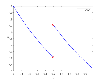
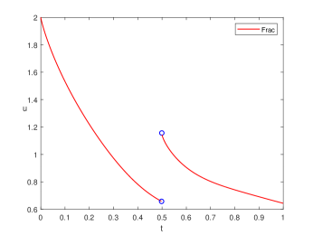
Figure 1. Plots of solutions: ordinary differential equation solutions (‘blue color’ or ‘left one’) and the variable-order fractional differential equation (‘red color’ or ‘right one’) with a same jump at $t=t_{0}=0.5$. As we can see, after the jump, the solution of the variable-order fractional differential equation depends on the past.

In this paper, we actually deal with a random analog of the above example. We will use a Poisson random measure to model jumps. There are two types of jumps, the first type are the “small jumps” and there are infinitely many of them in any finite time interval. We deal with the small jumps by compensating the jumps and the procedure is similar to the white noise case. For large jumps, we use the interlacing procedure, see chapter 2 of [2]. However, due to the memory term, we need a finer analysis as the above example.

1.3. Preliminaries and notation

Let $\big{(}\Omega,\mathcal{F},\{\mathcal{F}_{t}\}_{\geq 0},\mathbb{P}\big{)}$ be a filtered probability space and $N(dt,dz)$ be an $\mathcal{F}_{t}$-adapted Poisson random measure on $\mathbb{R}_{+}\times\mathbb{R}^{d}\backslash\{0\}$ with $N(0,\cdot)=0$ and with intensity measure $dt\nu(dx)$, where $\nu$ is a Lévy measure which means $\nu\{0\}=0$ and $\int_{\mathbb{R}^{d}}(1\wedge|x|^{2})\nu(dx)<\infty.$ The compensated Poisson random measure is defined as

$$\widetilde{N}(dt,dz):=N(dt,dz)-\nu(dz)dt$$

which is a martingale measure, see chapter 4 of [2] for the definition of martingale measure. Without loss of generality, for any $t\geq 0$, $\mathcal{F}_{t}$ can be chosen as the completion and augmentation of the filtration generated by the Poisson random measure.

The argument of this paper also works for $\mathbb{R}^{d}$-valued SDEs. Since we are mainly interested in the interplay of the memory term and the random noise, we concentrate on scalar SDEs.
Denote $\mathbb{R}_{+}:=[0,+\infty)$. We call the mappings $f:\mathbb{R}_{+}\times\mathbb{R}\rightarrow\mathbb{R},g:\mathbb{R}_{+}\times\mathbb{R}\times\mathbb{R}^{d}\backslash\{0\}\rightarrow\mathbb{R},h:\mathbb{R}_{+}\times\mathbb{R}\times\mathbb{R}^{d}\backslash\{0\}\rightarrow\mathbb{R}$ the drift, small jump, large jump coefficients, which are measurable functions. To ensure the predictability of the jump coefficients, we always have the following assumption:

Assumption (A0): For fixed $t\geq 0,z\in\mathbb{R}^{d}\backslash\{0\}$,

$$x\mapsto g(t,x,z)\mbox{ and }x\mapsto h(t,x,z),$$

are continuous functions.

The above assumption ensures the predictability of the jump coefficients. For any càdlàg process $\{U(t)\}_{t\geq 0}$, the following classes of functions will make the stochastic integral meaningful:

1. $\mathcal{L}:=\{\varphi:\mathbb{R}_{+}\times\mathbb{R}\times\mathbb{R}^{d}\backslash\{0\}\rightarrow\mathbb{R}:\forall t>0,\int_{0}^{t}\int_{\mathbb{R}^{d}\backslash\{0\}}|\varphi(s,U(s-),z)|N(ds,dz)<\infty,\ a.s.\}$

2. $\mathcal{L}^{p,loc}:=\{\varphi:\mathbb{R}_{+}\times\mathbb{R}\times\mathbb{R}^{d}\backslash\{0\}\rightarrow\mathbb{R}:\forall t>0,\int_{0}^{t}\int_{\mathbb{R}^{d}\backslash\{0\}}|\varphi(s,U(s-),z)|^{p}\nu(dz)ds<\infty,\ a.s.\}$, where $1\leq p\leq 2$.

See chapter 4 of [2] for a complete definition of the stochastic integral when the jump coefficients are in $\mathcal{L}$ and $\mathcal{L}^{i,loc},i=1,2$. For the case $1<p<2$, we use the standard truncating technique $\varphi=\varphi 1_{|\varphi|>1}+\varphi 1_{|\varphi|\leq 1}$ to define the integral.

For the variable-order time fractional integral operator defined by (10), if we integrate both sides of (9), we have the following integral form:

$$\begin{split}u(t)=&\ u_{0}+\int_{0}^{t}\kappa(t,s)u(s)ds+\int_{0}^{t}f\big{(}s,u(s)\big{)}ds\\ &\int_{0}^{t}\int_{|z|<1}g\big{(}s,u(s-),z\big{)}\widetilde{N}(ds,dz)+\int_{0}^{t}\int_{|z|\geq 1}h\big{(}s,u(s-),z\big{)}N(ds,dz),\end{split}$$ (12)

where

$$\kappa(t,s):=\frac{\lambda}{\Gamma(1-\alpha(t))(t-s)^{\alpha(t)}}.$$ (13)

Thus we have the following definition of (strong) solution to (9):

Definition 1.1.

We say an $\mathcal{F}_{t}-$adapted càdlàg process $\{u(t)\}_{t\geq 0}$ is a strong solution of (9) if for each $t>0$,

$$\int_{0}^{t}|\kappa(t,s)u(s)|ds,\int_{0}^{t}|f(s,u(s))|ds,\ \int_{0}^{t}\int_{|z|<1}g\big{(}s,u(s-),z\big{)}\widetilde{N}(ds,dz),$$

$$\int_{0}^{t}\int_{|z|\geq 1}|h(s,u(s-),z)|N(ds,dz).$$

are well-defined and finite $\mathbb{P}$-almost surely, and (12) holds $\mathbb{P}$ a.s.

We say the strong solution of (9) is (pathwise) unique if two solutions $\tilde{u}(t),u(t)$ with $u(0)=\tilde{u}(0)$ a.s. satisfy

$$\mathbb{P}(\tilde{u}(t)=u(t),\forall t\geq 0)=0.$$

In this paper, we always deal with strong solutions in the sense above. For simplicity, we will only speak of solutions from now on.

Notational convention: Throughout the paper, we use capital letters $C_{1}(\cdot),C_{2}(\cdot),\cdots$ to denote different constants in the statement of the results, the arguments inside the brackets are the parameters the constant depends on. The lowercase letters $c_{1}(\cdot),c_{2}(\cdot),\cdots$ will denote constants used in the proof, and we do not care about their values and they may be different from one appearance to another. They will start anew in every proof. The dependence of the integral coefficients $\alpha,\lambda,f,g,h$ will not be mentioned. Indeed, only the dependence on the power $p$ and time $T>0$ will be mentioned explicitly. $g$ is the small jump coefficient and is defined on $\mathbb{R}_{+}\times\mathbb{R}\times\{z:0<|z|<1\}$, we understand $g:\mathbb{R}_{+}\times\mathbb{R}\times\mathbb{R}^{d}\backslash\{0\}\rightarrow\mathbb{R}$ as $g(s,x,z)1_{\{z:0<|z|<1\}}(z)$. $h$ is the large jump coefficient and we understand it in a similar manner. The integral with respect to time $\int_{0}^{t}$ will always be understood as $\int_{(0,t]}$ in this paper.

2. Assumptions and statement of the theorem

Before we give the formal assumptions, we introduce the definition of $L^{p}$ Lipschitz continuity and $L^{p}$ linear growth condition for the jump coefficients.

Definition 2.1.

Let $p>0$. We say that the small jump coefficient $g:\mathbb{R}_{+}\times\mathbb{R}\times\{z\in\mathbb{R}^{d}:0<|z|<1\}\rightarrow\mathbb{R}$ is $L^{p}$ Lipschitz continuous if there is a locally bounded function $L(\cdot)$ defined on $[0,\infty)$ such that for any $t\geq 0,u\in\mathbb{R}$,

$$\int_{|z|<1}|g(t,u,z)-g(t,\tilde{u},z)|^{p}\nu(dz)\leq L(t)|u-\tilde{u}|^{p}.$$

We say that g satisfies the $L^{p}$ linear growth condition if there is a locally bounded function $L(\cdot)$ defined on $[0,\infty)$ such that for any $t\geq 0,u\in\mathbb{R}$,

$$\int_{|z|<1}|g(t,u,z)|^{p}\nu(dz)\leq L(t)(1+|u|^{p}).$$

We remark that $L^{2}$-Lipschitz continuity and $L^{2}$-linear growth condition are the same as the usual sense. Our assumptions on the coefficients are:
Assumption (A1) (Fractional order condition): The fractional order function $\alpha:\mathbb{R}_{+}\rightarrow[0,1)$ is a continuous function. Thus we can define its maximal function

$$\alpha^{*}(t):=\sup_{0\leq s\leq t}\alpha(s)\in[0,1),\ \forall t\geq 0.$$ (14)

Assumption (A2) (Lipschitz condition):
For some $p\in[1,2]$, the small jump coefficient $g$ is $L^{p}$-Lipschitz continuous, i.e., there is a locally bounded function $L(\cdot)$ defined on $[0,\infty)$ such that

$$\int_{|z|<1}|g(t,u,z)-g(t,\tilde{u},z)|^{p}\nu(dz)\leq L(t)|u-\tilde{u}|^{p},\quad t\geq 0,u,\tilde{u}\in\mathbb{R}.$$

The drift coefficient $f$ is also Lipschitz continuous, i.e., for the same locally bounded function $L(\cdot)$ above, it holds that

$$|f(t,u)-f(t,\tilde{u})|\leq L(t)|u-\tilde{u}|,\quad t\geq 0,u,\tilde{u}\in\mathbb{R}.$$

Assumption (A3) (Linear growth condition):
For the same $p\in[1,2]$ as in (A2), the small jump coefficient $g$ satisfies $L^{p}$-linear growth condition, i.e., there is a locally bounded function $L(\cdot)$ defined on $[0,\infty)$ such that for any $t\geq 0,u\in\mathbb{R}$,

$$\int_{|z|<1}|g(t,u,z)|^{p}\nu(dz)\leq L(t)(1+|u|^{p}).$$

The drift coefficient $f$ satisfies the linear growth condition, i.e., for the same locally bounded function $L(\cdot)$ above, it holds that

$$|f(t,u)|\leq L(t)(1+|u|),\quad t\geq 0,u\in\mathbb{R}.$$

Under the above assumptions, the well-posedness of the solution can be established: Under the above assumptions, we can prove the well-posedness of (9).

Theorem 2.2.

If Assumptions (A1)–(A3) hold, then there exists a unique solution to (9) for any given initial distribution $u_{0}\in\mathcal{F}_{0}$.

Remark 2.3.

(A2) can be weakened to non-Lipschitz coefficients as in [34]. However, the trick is also based on the classical approximating procedure, which is standard so we only consider the Lipschitz case. The non-trivial part is due to the presence of the memory term. Unlike in [12], we do not need any condition on the large jump term and the initial distribution.

If the initial distribution $u_{0}$ does not have finite moment, then we can not expect the solution to have finite moment. Thus to get $L^{p}$ moment estimates for the solution to (9), first we need to assume $\mathbb{E}(|u_{0}|^{p})<\infty$. Apart from that, we also need some assumptions on the large jump coefficients. The moment estimates of the solution to (9) are as follows:

Theorem 2.4.

Let $u(t)$ be a solution to (9).
Case 1: Suppose $1\leq p\leq 2$, $u_{0}\in L^{p}$ (i.e., $||u_{0}||_{p}^{p}:=\mathbb{E}|u_{0}|^{p}<\infty$), the drift coefficient $f$ satisfies the linear growth condition and the jump coefficients $g,h$ satisfy $L^{p}$ linear growth condition, i.e., there is a locally bounded function $L(\cdot)$ defined on $[0,\infty)$ such that for any $t\geq 0$ and $u\in\mathbb{R}$,

$$\begin{split}&|f(t,u)|\leq L(t)(1+|u|)\\ &\int_{|z|<1}|g(t,u,z)|^{p}\nu(dz)\leq L(t)(1+|u|^{p})\\ &\int_{|z|\geq 1}|h(t,u,z)|^{p}\nu(dz)\leq L(t)(1+|u|^{p})\end{split}$$

Then for any $T>0$, we have

$$\mathbb{E}\big{[}\sup_{0\leq t\leq T}|u(t)|^{p}\big{]}\leq C_{1}(p,T,||u_{0}||_{p})<\infty,$$ (15)

where

$$C_{1}(p,T,||u_{0}||_{p}):=c(p,T,||u_{0}||_{p})E_{1-\alpha^{*}(T),1}(c(p,T)\Gamma(1-\alpha^{*}(T))T^{1-\alpha^{*}(T)})<\infty,$$

and $E_{p,q}$ is the Mittag-Leffler function defined in Lemma 3.5.

Case 2: Suppose that $p\geq 2$, and that, in addition to the assumptions in Case 1, the small jump coefficient $g$ satisfies $L^{2}$ linear growth condition. Then (15) holds.

As an application of the moment estimates, we can establish the Hölder regularity of the solution $u(t)$ to (9). Hölder regularity means that for any two times $t_{1}\leq t_{2}$, usually $t_{2}-t_{1}$ is small, we have for some $p>0,\beta>0$,

$$\mathbb{E}|u(t_{2})-u(t_{1})|^{p}\leq c(p)|t_{2}-t_{1}|^{\beta}.$$

To establish the Hölder regularity of the solution to (9), we first need a more restrictive condition on the fractional order $\alpha(t)$:

Assumption (A1’): The fractional order function $\alpha:\mathbb{R}_{+}\rightarrow(0,1)$ is locally Hölder continuous with order $\gamma>0$, i.e., for any $T>0$, there exists $C_{2}(T)$, such that for any $0\leq t_{1}<t_{2}\leq T$,

$$|\alpha(t_{2})-\alpha(t_{1})|\leq C_{2}(T)|t_{2}-t_{1}|^{\gamma}.$$

Theorem 2.5.

Suppose $u(t)$ is a solution to (9) and that for some $p\geq 1$

$$\mathbb{E}\big{[}\sup_{0\leq t\leq T}|u(t)|^{p}\big{]}\leq C_{1}:=C_{1}(p,T,||u_{0}||_{p})<\infty.$$

We further assume that (A1’) holds, $f$ satisfies the linear growth condition and $g,h$ satisfy the $L^{p}$ linear growth condition. If $p\geq 2$, we also assume that $g$ satisfies the $L^{2}$ linear growth condition. Then for any $T>0$, there exists $C_{3}:=C_{3}(p,T)>0,C_{4}:=C_{4}(p,T)>0$ such that

$$\mathbb{E}|u(t_{2})-u(t_{1})|^{p}\leq C_{3}|t_{2}-t_{1}|^{C_{4}},0\leq t_{1}<t_{2}\leq T.$$ (16)

3. Existence and uniqueness of the solution

3.1. Some lemmas

Before we prove the existence and uniqueness, we summarize some frequently used results which are either easy to prove or already known. We will either give a quick proof or the reference to interested readers.

Lemma 3.1.

(Discrete Jesens’s inequality [21]) For any $a_{i}\in\mathbb{R}$ and $p>0$,

$$\Big{|}\sum_{i=1}^{m}a_{i}\Big{|}^{p}\leq\max\{m^{p-1},1\}\sum_{i=1}^{m}|a_{i}|^{p}.$$ (17)

We denote by $\mathbb{D}[0,\infty)$ the space of all càdlàg functions defined on $[0,+\infty)$ with values in $\mathbb{R}$. The natural topology is the Skorohod topology. We will not dig into that topology and only need the following simple lemma:

Lemma 3.2.

Let $f$ be a function on $[0,\infty)$. If $f_{n}(\cdot)$ is a sequence of càdlàg functions such that for all $T>0$, we have

$$\lim_{n\rightarrow\infty}\sup_{0\leq t\leq T}|f_{n}(t)-f(t)|=0,$$

then $f(\cdot)\in\mathbb{D}[0,\infty)$.

Proof.

Without loss of generality, we only prove the case for $t>0$. We would like to show that

$$\lim_{s\rightarrow t,s\geq t}f(s)=f(t)\mbox{ and }\lim_{s\rightarrow t,s<t}f(s)\mbox{ exists}.$$

We will only prove that $\lim_{s\rightarrow t,s<t}f(s)$ exists, because the proof of right continuity is similar. Indeed, for any $\varepsilon>0$ and fixed $t>0$, we have $N:=N(\varepsilon,t)>0$, such that

$$\sup_{0\leq s\leq t}|f_{N}(s)-f(s)|<\frac{\varepsilon}{2}.$$

For this $N$, there exists a $\delta:=\delta(\varepsilon,t)>0$, such that if $0\leq s_{1}<s_{2}<t$ and $t-s_{1}<\delta$,

$$|f_{N}(s_{2})-f_{N}(s_{1})|<\frac{\varepsilon}{2},|f_{N}(t-)-f_{N}(s)|<\frac{\varepsilon}{2}.$$

Thus

$$|f(s_{2})-f(s_{1})|\leq|f(s_{2})-f_{N}(s_{2})|+|f_{N}(s_{2})-f(s_{1})|<\varepsilon.$$

The proof is now complete. ∎

Lemma 3.3.

(Continuity of the Gamma function $\Gamma(x)$) Given $0<a<1<b$, for $x_{1},x_{2}\in(a,b)$, we have the local Lipschitz continuity of the Gamma function

$$|\Gamma(x_{2})-\Gamma(x_{1})|\leq L|x_{2}-x_{1}|.$$ (18)

Here $L:=L(a,b)$ is a constant.

Proof.

First, by the mean value theorem, there exists $\eta\in(x_{1},x_{2})$ such that

$$t^{x_{2}-1}-t^{x_{1}-1}=(\log t)t^{\eta-1}(x_{2}-x_{1}).$$

Then we have

$$|t^{x_{2}-1}-t^{x_{1}-1}|\leq|(\log t)(t^{a-1}+t^{b-1})|x_{2}-x_{1}|.$$ (19)

Using (19) we have

$$\begin{split}&|\Gamma(x_{2})-\Gamma(x_{1})|\leq\int_{0}^{\infty}|t^{x_{2}-1}-t^{x_{1}-1}|e^{-t}dt\leq|x_{2}-x_{1}|\int_{0}^{\infty}|(\log t)(t^{a-1}+t^{b-1})|e^{-t}dt\\ &\hskip 14.45377pt=|x_{2}-x_{1}|\Big{(}\int_{0}^{1}|(\log t)(t^{a-1}+t^{b-1})|e^{-t}dt+\int_{1}^{\infty}|(\log t)(t^{a-1}+t^{b-1})|e^{-t}dt\Big{)}\\ &\hskip 14.45377pt=:|x_{2}-x_{1}|\Big{(}G_{1}+G_{2}\Big{)}.\end{split}$$ (20)

By the fact that

$$\Big{|}\int_{0}^{1}t^{\gamma}\log t\ dt\Big{|}<\infty,\quad\gamma>-1,$$ (21)

we have

$$G_{1}=\int_{0}^{1}|(\log t)(t^{a-1}+t^{b-1})|e^{-t}dt\leq-\int_{0}^{1}\log t(t^{1-a}+t^{b-1})dt=\frac{1}{(2-a)^{2}}+\frac{1}{b^{2}}.$$ (22)

Let $\zeta:=\sup_{1\leq t<\infty}\{(\log t)(t^{a-1}+t^{b-1})|e^{-t/2}\}$, it is easy to see that $\zeta<+\infty$. Then by the definition of $\zeta$ we have

$$\begin{split}G_{2}&=\int_{1}^{\infty}|(\log t)(t^{a-1}+t^{b-1})|e^{-t}dt=\int_{1}^{\infty}|(\log t)(t^{a-1}+t^{b-1})|e^{-t/2}e^{-t/2}dt\\ &\leq\zeta\int_{1}^{\infty}e^{-t/2}dt=\frac{2\zeta}{\sqrt{e}}.\end{split}$$ (23)

Plugging (22) and (23) into (LABEL:Gamma:e2), we get

$$\begin{split}|\Gamma(x_{2})-\Gamma(x_{1})|\leq\Big{(}\frac{1}{(2-a)^{2}}+\frac{1}{b^{2}}+\frac{2\zeta}{\sqrt{e}}\Big{)}|x_{2}-x_{1}|=:L|x_{2}-x_{1}|.\end{split}$$ (24)

∎

Lemma 3.4.

Under (A1), for any $T>0$, there exist a constant $C_{5}(T)>0$ such that for any $0\leq s<t\leq T$,

$$|\kappa(t,s)|\leq C_{5}(T)(t-s)^{-\alpha^{*}(T)}.$$ (25)

Proof.

Recall the definition (10), and that $\Gamma(\cdot)$ is locally Lipschitz continuous on $(0,\infty)$, we have for $t-s\leq 1$,

$$|\kappa(t,s)|=\bigg{|}\frac{\lambda}{\Gamma(1-\alpha(t))}\bigg{(}\frac{1}{t-s}\bigg{)}^{\alpha(t)}\bigg{|}\leq c(T)(t-s)^{-\alpha^{*}(T)}.$$

For $t-s\geq 1$, we have

$$|\kappa(t,s)|\leq c_{1}(T)\leq c_{2}(T)(t-s)^{-\alpha^{*}(T)}$$

because $t-s\leq T$ and $(t-s)^{-\alpha^{*}(T)}\geq c_{3}(T)$. Taking $C_{5}(T)=\max\{c(T),c_{2}(T)\}$, we arrive at the desired assertion. ∎

Lemma 3.5.

(Gronwall type inequality) Suppose $\varphi(\cdot),\varphi_{0}(\cdot)$ are non-negative locally bounded function on $[0,\infty)$. If for any $0\leq a<b<\infty$, there exists $C_{6}\geq 0,0<\beta<1$, such that

$$\varphi(t)\leq\varphi_{0}(t)+C_{6}\int_{a}^{t}\varphi(s)(t-s)^{\beta-1}ds,\ \forall t\in[a,b)$$

then

$$\varphi(t)\leq\varphi_{0}(t)+\int_{a}^{t}\sum_{n=1}^{\infty}\frac{(C_{6}\Gamma(\beta))^{n}}{\Gamma(n\beta)}(t-s)^{n\beta-1}\varphi_{0}(s)ds,\ \forall t\in[a,b).$$ (26)

In particular, if $\varphi_{0}(\cdot)$ is non-decreasing, then

$$\varphi(t)\leq\varphi_{0}(t)E_{\beta,1}\big{(}C_{6}\Gamma(\beta)(t-a)^{\beta}\big{)},~{}~{}~{}\forall t\in[a,b),$$ (27)

where $E_{p,q}(z)$ is the Mittag-Leffler function defined by (see [10, 20, 28])

$$E_{p,q}(z):=\sum_{k=0}^{\infty}\frac{z^{k}}{\Gamma(pk+q)},\qquad z\in\mathbb{R},~{}~{}p\in\mathbb{R}^{+},~{}~{}q\in\mathbb{R}.$$

Proof.

See [31] for detailed proof. Or one can prove the result directly by iteration, and the computation in the proof Proposition 3.9. ∎

Lemma 3.6.

If $\theta:[0,+\infty)\rightarrow\mathbb{R}$ locally bounded and $\alpha^{*}\in[0,1)$, then for all $t>0$,

$$\sup_{0\leq s\leq t}\int_{0}^{s}\frac{|\theta(r)|}{(s-r)^{\alpha^{*}}}dr\leq\int_{0}^{t}\frac{\sup_{0\leq r\leq\tilde{u}}|\theta(r)|}{(t-\tilde{u})^{\alpha^{*}}}d\tilde{u}.$$ (28)

Proof.

For any $s\in[0,t]$, by the change of variables $u=r/s$, we have

$$\int_{0}^{s}\frac{|\theta(r)|}{(s-r)^{\alpha^{*}}}dr=s^{1-\alpha^{*}}\int_{0}^{1}\frac{|\theta(us)|}{(1-u)^{\alpha^{*}}}du\leq t^{1-\alpha^{*}}\int_{0}^{1}\frac{\sup_{0\leq r\leq ut}|\theta(r)|}{(1-u)^{\alpha^{*}}}du.$$

By the change of variable $\tilde{u}=ut$, the above is equal to

$$\int_{0}^{t}\frac{\sup_{0\leq r\leq\tilde{u}}|\theta(r)|}{(t-\tilde{u})^{\alpha^{*}}}d\tilde{u}.$$

∎

Lemma 3.7.

(Moment identities and estimates) Fix $T>0$. Suppose $g:\Omega\times[0,T]\times\{z:0<|z|<1\}\rightarrow\mathbb{R}$ and $h:\Omega\times[0,T]\times\{z:|z|\geq 1\}\rightarrow\mathbb{R}$ are predictable. Then we have the following:

1. (Itô’s isometry) If for any finite stopping time $\tau$, we have

   $$\mathbb{E}\big{[}\int_{0}^{\tau\wedge T}\int_{|z|<1}|g(s,z)|^{2}\nu(dz)ds\big{]}<\infty,$$

   then

   $$\mathbb{E}\Big{[}\int_{0}^{\tau\wedge T}\int_{|z|<1}|g(s,z)|^{2}ds\nu(dz)\Big{]}=\mathbb{E}\Big{[}\big{|}\int_{0}^{\tau\wedge T}\int_{|z|<1}g(s,z)\widetilde{N}(ds,dz)\big{|}^{2}\Big{]}.$$ (29)

2. For any $p\geq 2$, if

   $$\int_{0}^{T}\int_{|z|<1}|g(s,z)|^{2}ds\nu(dz)<\infty,\quad a.s.$$

   then there exists a $C_{7}(p)>0$ such that

   $$\mathbb{E}\sup_{0\leq t\leq T}\bigg{|}\int_{0}^{t}\int_{|z|<1}g(s,z)\widetilde{N}(ds,dz)\bigg{|}^{p}$$ (30)

   $$\leq C_{7}(p)\Bigg{[}\mathbb{E}\Big{(}\int_{0}^{T}\int_{|z|<1}|g(s,z)|^{2}ds\nu(dz))^{p/2}\Big{)}+\mathbb{E}\Big{(}\int_{0}^{T}\int_{|z|<1}|g(s,z)|^{p}ds\nu(dz)\Big{)}\bigg{]}.$$

3. For any $p\in[1,2]$, if

   $$\int_{0}^{T}\int_{|z|<1}|g(s,z)|^{p}ds\nu(dz)<\infty\quad a.s.$$

   then there exists a $C_{8}(p)>0$ such that

   $$\mathbb{E}\sup_{0\leq t\leq T}\big{|}\int_{0}^{t}\int_{|z|<1}g(s,z)\widetilde{N}(ds,dz)\big{|}^{p}\leq C_{8}(p)\mathbb{E}\int_{0}^{T}\int_{|z|<1}|g(s,z)|^{p}ds\nu(dz).$$ (31)

4. For any $p\geq 1$, if

   $$\int_{0}^{T}\int_{|z|\geq 1}|h(s,z)|^{p}ds\nu(dz)<\infty\quad a.s.$$

   then there exists a $C_{9}(p,T)>0$ such that

   $$\mathbb{E}\sup_{0\leq t\leq T}\big{|}\int_{0}^{t}\int_{|z|\geq 1}h(s,z)N(ds,dz)\big{|}^{p}\leq C_{9}(p,T)\mathbb{E}\int_{0}^{T}\int_{|z|\geq 1}|h(s,z)|^{p}ds\nu(dz).$$ (32)

Proof.

The above estimates are essentially due to [25]. To see the detailed proof of the above version, see [36]. ∎

Lemma 3.8.

(Structure of large jumps, [2, Chap. 2]) If $u(t)$ is an adapted càdlàg process, then

$$\int_{0}^{T}\int_{|z|\geq 1}h(t,u(t-),z)N(dt,dz)=\sum_{t=T_{j}\wedge T,j\geq 1}h(t,u(t-),P(t)),$$

where $P(t):=\int_{0}^{t}\int_{|z|\geq 1}zN(ds,dz)$ is an $\mathbb{R}^{d}$-valued compound Poisson process and $\{T_{n}\}_{n\geq 0}$ is defined by $T_{0}=0$, and for $n\geq 1$,

$$T_{n}:=\inf\{t>T_{n-1}:P(t)\neq P(t-)\}.$$

3.2. Proof of the existence and uniqueness

The outline of the proof is as follows:
Step I: First we assume the large coefficient$h(t,x,z)$ is 0, then the existence and uniqueness can be derived similarly as in the case of the classical fractional SDE if we assume $\mathbb{E}[|u_{0}|^{p}]<\infty$, where $p\in[1,2]$ is the constant in (A2). Indeed, we will prove a stronger version which implies the above result.

Step II: We show that the moment condition for $u_{0}$ can be dropped using a localization trick.

Step III: We use the interlacing procedure to glue together the large jumps.

Before we prove Theorem 2.2, we prove the following result which implies Step I, Step II and is needed in Step III.

Proposition 3.9.

Suppose that Assumptions (A1)–(A3) hold and $p\in[1,2]$ is as in (A2). Suppose also that $\{k(t)\}_{t\geq 0}$ is an adapted càdlàg process such that $\forall T>0$, we have

$$\mathbb{E}(\sup_{0\leq t\leq T}|k(t)|^{p})<\infty,$$

then the following stochastic integral equation

$$u(t)=\ k(t)+\int_{0}^{t}\kappa(t,s)u(s)ds+\int_{0}^{t}f\big{(}s,u(s)\big{)}ds+\int_{0}^{t}\int_{|z|<1}g\big{(}s,u(s-),z\big{)}\widetilde{N}(ds,dz)$$ (33)

has a unique strong solution, which is an adapted càdlàg process satisfying

$$\mathbb{E}\big{[}\sup_{0\leq t\leq T}|u(t)|^{p}\big{]}\leq C_{10}(p,T)\mathbb{E}\big{[}\sup_{0\leq t\leq T}|k(t)|^{p}\big{]}.$$

Moreover, if $\forall t\in[0,T],k(t)\in\mathcal{F}_{0}$, then the moment condition for $k(t)$ can be dropped, i.e., (33) has a unique solution even if

$$\mathbb{E}\big{[}\sup_{0\leq t\leq T}|k(t)|^{p}\big{]}=\infty.$$

Proof.

Fix an arbitrary $T>0$. We first prove the first assertion of the proposition.

Part I: Suppose $K(T,p):=\mathbb{E}\sup_{0\leq t\leq T}|k(t)|^{p}<\infty$. Define a sequence of approximation processes $\{u_{n}(t)\}_{n\geq 0}$ by $u_{0}(t):=k(t),\forall t\in[0,T]$ and for $n\geq 1$,

$$\begin{split}u_{n}(t):=&\ k(t)+\int_{0}^{t}\kappa(t,s)u_{n-1}(s)ds+\int_{0}^{t}f(s,u_{n-1}(s))ds+\int_{0}^{t}\int_{|z|<1}g(s,u_{n-1}(s-),z)\tilde{N}(ds,dz).\end{split}$$ (34)

By definition, each $u_{n}(t)$ is an adapted càdlàg process on $[0,T]$. Our goal is to establish a good decay rate as $n$ tends to infinity for

$$\mathbb{E}\big{[}\sup_{0\leq s\leq t}|u_{n}(s)-u_{n-1}(s)|^{p}\big{]}.$$

To establish the estimate for $\mathbb{E}(\sup_{0\leq s\leq t}|u_{n}(s)-u_{n-1}(s)|^{p})$, $n\geq 1$, we apply the discrete Jensen’s inequality,

$$\mathbb{E}\big{[}\sup_{0\leq s\leq t}|u_{n+1}(s)-u_{n}(s)|^{p}\big{]}$$

$$\leq c_{1}(p)\mathbb{E}\bigg{[}\sup_{0\leq s\leq t}\Big{(}\big{|}\int_{0}^{s}\kappa(s,r)(u_{n}(r)-u_{n-1}(r))dr\big{|}^{p}$$

$$+\big{|}\int_{0}^{s}f(r,u_{n}(r))-f(r,u_{n-1}(r))dr\big{|}^{p}$$

$$+\big{|}\int_{0}^{s}\int_{|z|<1}(g(r,u_{n}(r-),z)-g(r,u_{n-1}(r-),z))\tilde{N}(dr,dz)\big{|}^{p}\Big{)}\bigg{]}$$

$$=:(i)+(ii)+(iii).$$

Applying Hölder’s inequality, (25) and (28), we get

$$(i) =c_{1}(p)\mathbb{E}\Big{[}\sup_{0\leq s\leq t}\big{|}\int_{0}^{s}\kappa(s,r)(u_{n}(r)-u_{n-1}(r))dr\big{|}^{p}\Big{]}$$

$$=c_{1}(p)\mathbb{E}\Big{[}\sup_{0\leq s\leq t}\big{|}\int_{0}^{s}\kappa(s,r)^{1/p^{\prime}}\kappa(s,r)^{1/p}(u_{n}(r)-u_{n-1}(r))dr\big{|}^{p}\Big{]}$$

$$\leq c_{1}(p)(\int_{0}^{t}|\kappa(t,s)|ds)^{p/p^{\prime}}\mathbb{E}\Big{[}\sup_{0\leq s\leq t}\int_{0}^{s}|\kappa(s,r)||u_{n}(r)-u_{n-1}(r)|^{p}dr\Big{]}$$

$$\leq c_{2}(p,T)(\int_{0}^{t}\frac{1}{|t-s|^{\alpha^{*}(T)}}ds)^{p/p^{\prime}}\mathbb{E}\Big{[}\sup_{0\leq s\leq t}\int_{0}^{s}\frac{|u_{n}(r)-u_{n-1}(r)|^{p}}{(s-r)^{\alpha^{*}(T)}}dr\Big{]}$$

$$\leq c_{3}(p,T)\int_{0}^{t}\frac{\mathbb{E}\big{[}\sup_{0\leq r\leq s}|u_{n}(r)-u_{n-1}(r)|^{p}\big{]}}{(t-s)^{\alpha^{*}(T)}}ds.$$

For $(ii)$, by Hölder’s inequality and the Lipschitz condition (A2), we have

$$(ii) =c_{1}(p)\mathbb{E}\Big{[}\sup_{0\leq s\leq t}\big{|}\int_{0}^{s}f(r,u_{n}(r))-f(r,u_{n-1}(r))dr\big{|}^{p}\Big{]}$$

$$\leq c_{4}(p,T)\int_{0}^{t}\mathbb{E}\Big{[}\sup_{0\leq r\leq s}|u_{n}(r)-u_{n-1}(r)|^{p}\Big{]}ds.$$

For $(iii)$, by applying the $L^{p}$ Lipschitz condition (A2), we have

$$\int_{0}^{T}\int_{|z|<1}|g(r,u_{n}(s),z)-g(r,u_{n-1}(s),z)|^{p}\nu(dz)ds\leq c_{5}(T)\int_{0}^{T}|u_{n}(s)-u_{n-1}(s)|^{p}ds<\infty,\ a.s.$$

because $\{u_{n}(t)\}_{0\leq t\leq T}$ are all càdlàg processes thus locally bounded a.s.. Then we apply (31) and the $L^{p}$ Lipschitz condition (A2) to get

$$(iii) =c_{1}(p)\mathbb{E}\Big{[}\sup_{0\leq s\leq t}\big{|}\int_{0}^{s}\int_{|z|<1}(g(r,u_{n}(r-),z)-g(r,u_{n-1}(r-),z))\tilde{N}(dr,dz)\big{|}^{p}\Big{]}$$

$$\leq c_{6}(p)\mathbb{E}\int_{0}^{t}\int_{|z|<1}|g(r,u_{n}(r-),z)-g(r,u_{n-1}(r-),z)|^{p}\nu(dz)ds$$

$$\leq c_{7}(p)\int_{0}^{t}\mathbb{E}\big{[}\sup_{0\leq r\leq s}|u_{n}(r)-u_{n-1}(r)|^{p}\big{]}ds.$$

Since for any $t\in[0,T]$ and $0\leq s\leq t$, we have $1\leq\frac{T^{\alpha^{*}(T)}}{(t-s)^{\alpha^{*}(T)}}$. Combining the estimates for $(i),(ii),(iii)$, we get

$$\mathbb{E}\big{[}\sup_{0\leq s\leq t}|u_{n+1}(s)-u_{n}(s)|^{p}\big{]}\leq c_{8}(p,T)\int_{0}^{t}\frac{\mathbb{E}\big{[}\sup_{0\leq r\leq s}|u_{n}(r)-u_{n-1}(r)|^{p}\big{]}}{(t-s)^{\alpha^{*}(T)}}ds.$$ (35)

Following the same argument, using the linear growth condition (A3) instead of the Lipschitz condition, we have

$$\mathbb{E}\big{[}\sup_{0\leq s\leq t}|u_{1}(s)-u_{0}(s)|^{p}\big{]}\leq c_{9}(p,T)\int_{0}^{t}\frac{\mathbb{E}\big{[}\sup_{0\leq r\leq s}|k(r)|^{p}\big{]}}{(t-s)^{\alpha^{*}(T)}}ds.$$ (36)

Now we define

$$K(t,p):=\mathbb{E}\big{[}\sup_{0\leq s\leq t}|k(s)|^{p}\big{]},\ 0\leq t\leq T,$$ (37)

$$g_{n}(t):=\mathbb{E}\big{[}\sup_{0\leq s\leq t}|u_{n}(s)-u_{n-1}(s)|^{p}\big{]},n\geq 1.$$

It follows from (36) that

$$g_{1}(t)\leq c_{9}(p,T)K(T,p)\int_{0}^{t}\frac{1}{(t-s)^{\alpha^{*}(T)}}ds=c_{10}(p,T)K(T,p)t^{1-\alpha^{*}(T)}.$$ (38)

For simplicity, we set $c_{11}:=c_{11}(p,T):=\max\{c_{8}(p,T),c_{10}(p,T)\},\alpha^{*}:=\alpha^{*}(T)$. Then by (35), we have for all $n\geq 1$,

$$g_{n+1}(t)\leq c_{11}\int_{0}^{t}\frac{g_{n}(s)}{(t-s)^{\alpha^{*}}}ds.$$ (39)

Plugging (38) into (39), we get

$$g_{2}(t)\leq c_{11}^{2}K(T,p)\int_{0}^{t}\frac{s^{1-\alpha^{*}}}{(t-s)^{\alpha^{*}}}ds=c_{11}^{2}t^{2(1-\alpha^{*})}B(2-\alpha^{*},1-\alpha^{*})K(T,p),$$

where $B$ is the Beta function defined as

$$B(x,y):=\int_{0}^{1}s^{x-1}(1-s)^{y-1}ds,\quad x,y>0.$$

Suppose that for $n\geq 2$, we have

$$g_{n}(t)\leq c_{11}^{n}t^{n(1-\alpha^{*})}\prod_{i=2}^{n}B(i-(i-1)\alpha^{*},1-\alpha^{*})K(T,p),$$

then by induction, we have

$$g_{n+1}(t) \leq c_{11}\int_{0}^{t}\frac{g_{n}(s)}{(t-s)^{\alpha^{*}}}ds$$

$$\leq c_{11}^{n+1}\prod_{i=2}^{n}B(i-(i-1)\alpha^{*},1-\alpha^{*})K(T,p)\int_{0}^{t}\frac{s^{n(1-\alpha^{*})}}{(t-s)^{\alpha^{*}}}ds$$

$$=c_{11}^{n+1}\prod_{i=2}^{n}B(i-(i-1)\alpha^{*},1-\alpha^{*})K(T,p)t^{(n+1)(1-\alpha^{*})}\int_{0}^{1}s^{n+1-n\alpha^{*}-1}(1-s)^{1-\alpha^{*}-1}ds$$

$$=c_{11}^{n+1}t^{(n+1)(1-\alpha^{*})}\prod_{i=2}^{n+1}B(i-(i-1)\alpha^{*},1-\alpha^{*})K(T,p).$$

Recall that

$$B(x,y)=\frac{\Gamma(x)\Gamma(y)}{\Gamma(x+y)}.$$

Then for $n\geq 2$,

$$\prod_{i=2}^{n}B(i-(i-1)\alpha^{*},1-\alpha^{*})=\frac{\Gamma(2-\alpha^{*})\Gamma(1-\alpha^{*})^{n-1}}{\Gamma(n+1-n\alpha^{*})}=\frac{(1-\alpha^{*})\Gamma(1-\alpha^{*})^{n}}{\Gamma(1+n(1-\alpha^{*}))}.$$

In summary, the estimate for $g_{n}(t),n\geq 1$ is given as

$$g_{n}(t):=\mathbb{E}\big{[}\sup_{0\leq s\leq t}|u_{n}(s)-u_{n-1}(s)|^{p}\big{]}\leq\frac{[c_{11}\Gamma(1-\alpha^{*})t^{1-\alpha^{*}}]^{n}}{\Gamma(1+n(1-\alpha^{*}))}(1-\alpha^{*})K(T,p).$$ (40)

By Chebyshev’s inequality, we have

$$\sum_{n\geq 1}\mathbb{P}(\sup_{0\leq s\leq t}|u_{n}(s)-u_{n-1}(s)|>2^{-n})$$

$$\leq\sum_{n\geq 1}\frac{[2^{p}c_{11}\Gamma(1-\alpha^{*})t^{1-\alpha^{*}}]^{n}}{\Gamma(1+n(1-\alpha^{*}))}(1-\alpha^{*})K(T,p)<\infty.$$

The finiteness of the sum follows from the asymptotic behavior of $\Gamma$:

$$\Gamma(1+n(1-\alpha^{*}))\sim\sqrt{n(1-\alpha^{*})}\big{(}\frac{n(1-\alpha^{*})}{e}\big{)}^{n(1-\alpha^{*})}.$$

It follows from the Borel-Cantelli lemma and a standard limiting argument that there exists an adapted càdlàg process $u(t),0\leq t\leq T$, such that

$$\lim_{n\rightarrow\infty}\sup_{0\leq t\leq T}|u_{n}(t)-u(t)|=0,\mathbb{P}-a.s..$$

To show that $u(t)$ is actually a solution, we also need $L^{p}$ convergence. To this end, we define a norm on all the adapted càdlàg processes defined on $[0,T]$ as follows:

$$||v||_{p,T}:=\big{(}\mathbb{E}[\sup_{0\leq t\leq T}|v(t)|^{p}]\big{)}^{1/p}.$$

Denote

$$L^{p}([0,T]):=\{v:||v||_{p,T}<\infty\}.$$

It is easy to check that $L^{p}([0,T])$ is a Banach space. By (40), $\{u_{n}(t)\}$ form a Cauchy sequence in $L^{p}([0,T])$ because

$$\sum_{n\geq 1}\bigg{(}\frac{[c_{11}\Gamma(1-\alpha^{*})T^{1-\alpha^{*}}]^{n}}{\Gamma(1+n(1-\alpha^{*}))}\bigg{)}^{1/p}<\infty.$$

The limit coincides with the a.s. limit $u(t)$ and the convergence rate is given as

$$||u_{n}-u||_{p,T}\leq\sum_{k\geq n+1}\bigg{(}\frac{[c_{11}\Gamma(1-\alpha^{*})T^{1-\alpha^{*}}]^{k}}{\Gamma(1+k(1-\alpha^{*}))}(1-\alpha^{*})K(T,p)\bigg{)}^{1/p}\rightarrow 0.$$

To show that $u(t)$ is the solution, we define

$$\tilde{u}(t):=k(t)+\int_{0}^{t}\kappa(t,s)u(s)ds+\int_{0}^{t}f\big{(}s,u(s)\big{)}ds+\int_{0}^{t}\int_{|z|<1}g\big{(}s,u(s-),z\big{)}\widetilde{N}(ds,dz).$$

If we can show that

$$||u_{n}-\tilde{u}||_{p,T}\rightarrow 0,$$

then we have

$$\sup_{0\leq t\leq T}|\tilde{u}(t)-u(t)|=0,a.s.$$

which implies that $u(t)$ is a strong solution. To show $||u_{n}-\tilde{u}||_{p,T}\rightarrow 0$, by a similar argument as above, we have the following:

$$||u_{n}-\tilde{u}||_{p,T}^{p}=\mathbb{E}\big{[}\sup_{0\leq t\leq T}|u_{n}(t)-\tilde{u}(t)|^{p}\big{]}\leq c_{12}(p,T)\int_{0}^{T}\frac{||u_{n-1}-u||_{p,T}^{p}}{(T-t)^{\alpha^{*}}}dt\rightarrow 0,$$

because $||u_{n-1}-u||_{p,T}^{p}$ tends to $0$ as $n\to\infty$. Thus we showed that $u(t)$ is actually a strong solution of (9).
A by-product of the argument above is that we can directly get the moment estimate of $u$:

$$\mathbb{E}\big{[}\sup_{0\leq t\leq T}|u(t)|^{p}\big{]}=||u||_{p,T}^{p}$$

$$\leq\big{(}\sum_{n\geq 1}||u_{n}-u_{n-1}||_{p,T}+||u_{0}||_{p,T}\big{)}^{p}$$

$$\leq\bigg{\{}\sum_{n\geq 1}\bigg{(}\frac{[c_{11}\Gamma(1-\alpha^{*})T^{1-\alpha^{*}}]^{n}}{\Gamma(1+n(1-\alpha^{*}))}(1-\alpha^{*})K(T,p)\bigg{)}^{1/p}+K(T,p)^{1/p}\bigg{\}}^{p}$$

$$:=c_{13}(p,T)K(T,p)<\infty.$$

To finish the first part, it remains to show that if $u,v$ are two strong solutions with the same initial condition, then they must be the same. Indeed, if we denote $h(t):=||u-v||_{p,t}^{p}$, then by a similar argument,

$$h(T):=||u-v||_{p,T}^{p}\leq c_{14}(p,T)\int_{0}^{T}\frac{h(t)}{(T-t)^{\alpha^{*}}}dt.$$

then by the generalized Gronwall’s inequality (27), we have $u=v,a.s.$, i.e., the solution is unique. Thus we have finished the first part of the proposition under the assumption

$$K(T,p):=\mathbb{E}\sup_{0\leq t\leq T}|k(t)|^{p}<\infty.$$

Part II: $K(T,p):=\mathbb{E}\sup_{0\leq t\leq T}|k(t)|^{p}=\infty$, but we have $\forall t\geq 0,k(t)\in\mathcal{F}_{0}$
Denote

$$\Omega_{N}:=\{\sup_{0\leq t\leq T}|k(t)|\leq N\}\in\mathcal{F}_{0},\quad N\geq 1.$$

We have

$$\Omega=\bigcup_{N\geq 1}\Omega_{N},\mathbb{P}-a.s.$$

Indeed, since $k(t)$ is a càdlàg process, for almost all $\omega\in\Omega$, $k(t)(\omega)$ is a càdlàg function, which is bounded on $[0,T]$, and we must have $\omega$ is in some $\Omega_{N}$, which implies $\Omega\subset\bigcup_{N\geq 1}\Omega_{N},\mathbb{P}-a.s.$. The other direction is obvious.
From Part I, we know that for any $N\geq 1$, the following stochastic integral equation

$$w(t)=k(t)1_{\Omega_{N}}+\int_{0}^{t}\kappa(t,s)w(s)ds+\int_{0}^{t}f\big{(}s,w(s)\big{)}ds+\int_{0}^{t}\int_{|z|<1}g\big{(}s,w(s-),z\big{)}\widetilde{N}(ds,dz)$$ (41)

has a unique solution which is càdlàg and adapted, and we denote it as $u^{N}(t),t\in[0,T]$. Thus we can define $u(t)(\omega):=u^{N}(t)(\omega)$ if $\omega\in\Omega_{N},\forall t\in[0,T]$. First we need to show that $u(t)$ is well-defined. It is equivalent to show that if $M>N$, for $\mathbb{P}$-almost all $\omega\in\Omega_{N}\subset\Omega_{M}$, we have $u^{N}(t)(\omega)=u^{M}(t)(\omega),\forall t\in[0,T]$. Indeed, we have

$$\mathbb{E}\big{[}\sup_{0\leq t\leq T}|u^{N}(t)-u^{M}(t)|^{p}1_{\Omega_{N}}\big{]}$$

$$\leq c_{1}(p)\mathbb{E}\bigg{[}\sup_{0\leq t\leq T}\Big{(}\big{|}\int_{0}^{t}\kappa(t,s)(u^{N}(s)-u^{M}(s))ds\big{|}^{p}1_{\Omega_{N}}$$

$$+\big{|}\int_{0}^{t}\big{(}f(s,u^{N}(s))-f(s,u^{M}(s))\big{)}ds\big{|}^{p}1_{\Omega_{N}}$$

$$+\big{|}\int_{0}^{t}\int_{|z|<1}\big{(}g(s,u^{N}(s-),z)-g(s,u^{M}(s-),z)\big{)}\widetilde{N}(ds,dz)\big{|}^{p}1_{\Omega_{N}}\Big{)}\bigg{]}.$$

For the first two integrals, the indicator function $1_{\Omega_{N}}$ can be put inside because the integral is pathwisely defined. For the stochastic integral, we use the following “stopping time argument”: Define a stopping time (it is a stopping time because $k(t)\in\mathcal{F}_{0},\ \forall t\geq 0$)

$$T_{N}(\omega)=\begin{cases}0,&\omega\notin\Omega_{N},\\ \infty,&\omega\in\Omega_{N}.\end{cases}$$

Then we have $\forall t\in(0,T]$,

$$1_{\Omega_{N}}=1_{\{T_{N}=\infty\}}=1_{\{T_{N}\geq t\}}.$$ (42)

Now we use the following lemma, whose proof will be given later, to put the indicator function inside the integral:

Lemma 3.10.

Suppose $g$ is in $\mathcal{L}^{p,loc}$ for the above $p\in[1,2]$, i.e.,

$$\int_{0}^{T}\int_{\{z:|z|<1\}}|g(s,z)|^{p}\nu(dz)ds<\infty,\ a.s.$$

Then we have for any $t\in[0,T]$,

$$\int_{0}^{t}\int_{|z|<1}g(s,z)\widetilde{N}(ds,dz)1_{\Omega_{N}}=\int_{0}^{t}\int_{|z|<1}g(s,z)1_{\Omega_{N}}\widetilde{N}(ds,dz).$$ (43)

By the lemma above,

$$\big{|}\int_{0}^{t}\int_{|z|<1}\big{(}g(s,u^{N}(s-),z)-g(s,u^{M}(s-),z)\big{)}\widetilde{N}(ds,dz)\big{|}^{p}1_{\Omega_{N}}$$

$$=\big{|}\int_{0}^{t}\int_{|z|<1}\big{(}g(s,u^{N}(s-),z)-g(s,u^{M}(s-),z)\big{)}1_{\Omega_{N}}\widetilde{N}(ds,dz)\big{|}^{p}.$$

As argued in the proof of the first assertion, we have

$$\mathbb{E}\Big{[}\sup_{0\leq t\leq T}|u^{N}(t)-u^{M}(t)|^{p}1_{\Omega_{N}}\Big{]}\leq c_{2}(p,T)\int_{0}^{T}\sup_{0\leq r\leq s}\frac{\mathbb{E}\big{[}|u^{N}(r)-u^{M}(r)|^{p}1_{\Omega_{N}}\big{]}}{(T-s)^{\alpha^{*}}}ds.$$

Thus by the generalized Gronwall’s inequality we have

$$\sup_{0\leq t\leq T}\big{|}u^{N}(t)-u^{M}(t)\big{|}1_{\Omega_{N}}=0,\mathbb{P}-a.s.$$

which shows that $u(t)$ is well-defined.

It remains to show that $u(t)$ is the unique solution to (33). First we show that it is actually a solution. Indeed, for any $N\geq 1$, using (43) twice, we have

$$u(t)1_{\Omega_{N}}= \ u^{N}(t)1_{\Omega_{N}}=k(t)1_{\Omega_{N}}+\big{\{}\int_{0}^{t}\kappa(t,s)u^{N}(s)ds+\int_{0}^{t}f\big{(}s,u^{N}(s)\big{)}ds$$

$$+\int_{0}^{t}\int_{|z|<1}g\big{(}s,u^{N}(s-),z\big{)}\widetilde{N}(ds,dz)\big{\}}1_{\Omega_{N}}$$

$$= \ k(t)1_{\Omega_{N}}+\int_{0}^{t}\kappa(t,s)u^{N}(s)1_{\Omega_{N}}ds+\int_{0}^{t}f\big{(}s,u^{N}(s)\big{)}1_{\Omega_{N}}ds$$

$$+\int_{0}^{t}\int_{|z|<1}g\big{(}s,u^{N}(s-),z\big{)}1_{\Omega_{N}}\widetilde{N}(ds,dz)$$

$$= \ \Big{[}k(t)+\int_{0}^{t}\kappa(t,s)u(s)ds+\int_{0}^{t}f\big{(}s,u(s)\big{)}ds$$

$$\ +\int_{0}^{t}\int_{|z|<1}g\big{(}s,u(s-),z\big{)}\widetilde{N}(ds,dz)\Big{]}1_{\Omega_{N}}.$$

Thus (33) holds on every $\Omega_{N}$ thus on $\Omega=\bigcup_{N\geq 1}\Omega_{N}$ which implies that $u(t)$ is actually a solution.

Step II would be finished if we can show the solution of (33) is unique. Indeed, suppose $v(t)$ is also a solution with the same initial condition, then we claim that for all $N\geq 1$, $v(t)=u^{N}(t)$, $\mathbb{P}-$a.s. on $\Omega_{N},\forall t\in[0,T]$. If the claim is true, we know that $v(t)$ coincides with $u(t)$, $\mathbb{P}-$a.s. and the proof would be complete.

Now we prove by contradiction: suppose the claim is not true. In other words, there exists an $N\geq 1$, such that $v(t)$ and $u^{N}(t)$ are not the same on $\Omega_{N}$. Then we can construct another càdlàg process $\widetilde{v}(t)$ defined as

$$\widetilde{v}(t)=v(t)1_{\Omega_{N}}+u^{N}(t)1_{\Omega_{N}^{c}}.$$ (44)

$\widetilde{v}(t)$ is adapted because $1_{\Omega_{N}}\in\mathcal{F}_{0}$. We claim that $\widetilde{v}(t)$ is a solution to (41), which contradicts the fact that (41) has only one solution.

Indeed, if $\omega\in\Omega_{N}$, we have $1_{\Omega_{N}}(\omega)=1$. From our assumption that $v(t)$ is a solution to (33), we have $\mathbb{P}-a.s.$

$$\widetilde{v}(t)(\omega)= v(t)(\omega)=k(t)1_{\Omega_{N}}(\omega)+\int_{0}^{t}\kappa(t,s)v(s)ds1_{\Omega_{N}}(\omega)+\int_{0}^{t}f\big{(}s,v(s)\big{)}ds1_{\Omega_{N}}(\omega)$$

$$+\int_{0}^{t}\int_{|z|<1}g\big{(}s,v(s-),z\big{)}\widetilde{N}(ds,dz)1_{\Omega_{N}}(\omega)$$

$$= \ k(t)1_{\Omega_{N}}(\omega)+\int_{0}^{t}\kappa(t,s)v(s)1_{\Omega_{N}}ds(\omega)+\int_{0}^{t}f\big{(}s,v(s)\big{)}1_{\Omega_{N}}ds(\omega)$$

$$+\int_{0}^{t}\int_{|z|<1}g\big{(}s,v(s-),z\big{)}1_{\Omega_{N}}\widetilde{N}(ds,dz)(\omega)$$

$$= \ k(t)1_{\Omega_{N}}(\omega)+\int_{0}^{t}\kappa(t,s)\widetilde{v}(s)ds(\omega)+\int_{0}^{t}f\big{(}s,\widetilde{v}(s)\big{)}ds(\omega)$$

$$+\int_{0}^{t}\int_{|z|<1}g\big{(}s,\widetilde{v}(s-),z\big{)}\widetilde{N}(ds,dz)(\omega),$$

where in the last equality, we used (43) and (44):

$$\int_{0}^{t}\int_{|z|<1}g\big{(}s,\widetilde{v}(s-),z\big{)}\widetilde{N}(ds,dz)(\omega)$$

$$=\int_{0}^{t}\int_{|z|<1}g\big{(}s,v(s-),z\big{)}1_{\Omega_{N}}\widetilde{N}(ds,dz)(\omega)+\int_{0}^{t}\int_{|z|<1}g\big{(}s,u^{N}(s-),z\big{)}1_{\Omega_{N}^{c}}\widetilde{N}(ds,dz)(\omega)$$

$$=\int_{0}^{t}\int_{|z|<1}g\big{(}s,v(s-),z\big{)}1_{\Omega_{N}}\widetilde{N}(ds,dz)(\omega)+\int_{0}^{t}\int_{|z|<1}g\big{(}s,u^{N}(s-),z\big{)}\widetilde{N}(ds,dz)1_{\Omega_{N}^{c}}(\omega)$$

$$=\int_{0}^{t}\int_{|z|<1}g\big{(}s,v(s-),z\big{)}1_{\Omega_{N}}\widetilde{N}(ds,dz)(\omega)$$

If $\omega\in\Omega_{N}^{c}$, following the same argument with $1_{\Omega_{N}}$ replaced by $1_{\Omega_{N}^{c}}$, we get

$$\widetilde{v}(t)(\omega) =k(t)1_{\Omega_{N}}(\omega)+\int_{0}^{t}\kappa(t,s)\widetilde{v}(s)ds(\omega)+\int_{0}^{t}f\big{(}s,\widetilde{v}(s)\big{)}ds(\omega)$$

$$+\int_{0}^{t}\int_{|z|<1}g\big{(}s,\widetilde{v}(s-),z\big{)}\widetilde{N}(ds,dz)(\omega)$$

Thus $\widetilde{v}(t)$ is a solution to (41), a contradiction! The proof of the proposition is now complete. ∎

Proof of Lemma 3.10. We only need to deal with the case $t>0$. First we use the standard approximation in chapter 4 of [2]: suppose $A_{n}$ increases to $\{z:|z|<1\}$, and $\nu(A_{n})<\infty,\forall n\geq 1$. Then we have

$$\int_{0}^{t}\int_{A_{n}}g(s,z)\widetilde{N}(ds,dz)1_{\Omega_{N}}\rightarrow\int_{0}^{t}\int_{|z|<1}g(s,z)\widetilde{N}(ds,dz)1_{\Omega_{N}}$$

in probability. The right-hand side of (43) can be dealt with similarly. Thus we only need to show the following for any $n\geq 1$:

$$\int_{0}^{t}\int_{A_{n}}g(s,z)\widetilde{N}(ds,dz)1_{\Omega_{N}}=\int_{0}^{t}\int_{A_{n}}g(s,z)1_{\Omega_{N}}\widetilde{N}(ds,dz)$$ (45)

To prove (45), we use the definition of the integral. Recall $\nu(A_{n})<\infty$, by applying Lemma 3.8, we can define $P^{n}(t)=\int_{0}^{t}\int_{A_{n}}zN(ds,dz)$, which is a compound Poisson process. Define $\{T_{j}^{n}\}_{j\geq 1}$ by $T_{0}^{n}=0$ and for $j\geq 1$,

$$T_{j}^{n}:=\inf\{t>T_{j-1}^{n}:P^{n}(t)\neq P^{n}(t-)\}$$

Then the left-hand side of (45) is equal to

$$\int_{0}^{t}\int_{A_{n}}g(s,z)\widetilde{N}(ds,dz)1_{\Omega_{N}} =\big{[}\sum_{s\leq t\wedge T_{j}^{n},j\geq 1}g(s,\Delta P(s))\big{]}1_{\Omega_{N}}-\int_{0}^{t}\int_{A_{n}}g(s,z)\nu(dz)ds1_{\Omega_{N}}$$

$$=\big{[}\sum_{s\leq t\wedge T_{j}^{n},j\geq 1}g(s,\Delta P(s))\big{]}1_{\{T_{N}\geq t\}}-\int_{0}^{t}\int_{A_{n}}g(s,z)1_{\Omega_{N}}\nu(dz)ds$$

$$=\sum_{s\leq t\wedge T_{j}^{n}\wedge T_{N},j\geq 1}g(s,\Delta P(s))-\int_{0}^{t}\int_{A_{n}}g(s,z)1_{\Omega_{N}}\nu(dz)ds$$

$$=\sum_{s\leq t\wedge T_{j}^{n},j\geq 1}\big{[}g(s,\Delta P(s))1_{T_{N}\geq s}\big{]}-\int_{0}^{t}\int_{A_{n}}g(s,z)1_{\Omega_{N}}\nu(dz)ds$$

$$=\sum_{s\leq t\wedge T_{j}^{n},j\geq 1}\big{[}g(s,\Delta P(s))1_{\Omega_{N}}\big{]}-\int_{0}^{t}\int_{A_{n}}g(s,z)1_{\Omega_{N}}\nu(dz)ds$$

$$=\int_{0}^{t}\int_{A_{n}}g(s,z)1_{\Omega_{N}}\widetilde{N}(ds,dz)$$

where we used (42) several times. Here we remark that $1_{\Omega_{N}}\in\mathcal{F}_{0}$ thus $g(s,z)1_{\Omega_{N}}$ is still predictable. Thus (45) is true, and the proof of the lemma is complete. ∎

Now we prove the existence and uniqueness.

Proof of Theorem 2.2. Taking $k(t)\equiv u_{0}$ in Proposition 3.9, we immediately get Step I and Step II.
Step III: Suppose $h\neq 0$.
From Lemma 3.8 we have a sequence of strictly increasing stopping times $\{T_{n}\}_{n\geq 0}$, we can construct the solution inductively. From Step II, define $v_{0}(t)$ to be the unique solution to

$$v(t)=u_{0}+\int_{0}^{t}\kappa(t,s)v(s)ds+\int_{0}^{t}f(s,v(s))ds+\int_{0}^{t}\int_{|z|<1}g(s,v(s-),z)\widetilde{N}(ds,dz),$$

then we define $u(t),t\in[0,T_{1}]$ as

$$u(t)=\begin{cases}v_{0}(t),&t<T_{1},\\ v_{0}(T_{1}-)+h(T_{1},v_{0}(T_{1}-),\Delta P(T_{1})),&t=T_{1}.\end{cases}$$

After the first jump, the memory term comes into play. Since

$$T_{1},P(T_{1})\in\mathcal{F}_{T_{1}},\sigma\{v_{0}(t):0\leq t<T_{1}\}\subset\mathcal{F}_{T_{1}},$$

we have

$$k_{1}(t) :=u_{0}+\int_{0}^{T_{1}}\kappa(t,s)v_{0}(s)ds+\int_{0}^{T_{1}}f(s,u(s))ds$$

$$+\int_{0}^{T_{1}}\int_{|z|<1}g(s,u(s-),z)\widetilde{N}(ds,dz)+h(T_{1},v_{0}(T_{1}-),\Delta P(T_{1}))$$

is $\mathcal{F}_{T_{1}}$-measurable for any $t\geq T_{1}$. Then applying Proposition 3.9, replacing $\mathcal{F}_{0}$ by $\mathcal{F}_{T_{1}}$ in our case, the following equation

$$v(t)=k_{1}(t)+\int_{T_{1}}^{t}\kappa(t,s)v(s)ds+\int_{T_{1}}^{t}f(s,v(s))ds+\int_{T_{1}}^{t}\int_{|z|<1}g(s,v(s-),z)\widetilde{N}(ds,dz)$$

has a unique solution $v_{1}(t)$ on $[T_{1},\infty)$. Define $u(t)$ on $[T_{1},T_{2}]$ as

$$u(t)=\begin{cases}v_{1}(t),&T_{1}\leq t<T_{2},\\ v_{1}(T_{2}-)+h(T_{2},v_{1}(T_{2}-),\Delta P(T_{2})),&t=T_{2}.\end{cases}$$

Suppose we already defined the solution $u(t)$ on $[0,T_{n}],n\geq 2$, and $v_{i}(t),1\leq i\leq n-1$, then we define

$$k_{n}(t):= u_{0}+\int_{0}^{T_{n}}\kappa(t,s)u(s)ds+\int_{0}^{T_{n}}f(s,u(s))ds$$

$$+\int_{0}^{T_{n}}\int_{|z|<1}g(s,u(s-),z)\widetilde{N}(ds,dz)+\sum_{i=1}^{n}h(T_{i},v_{i-1}(T_{i}-),\Delta P(T_{i})).$$

The following equation

$$v(t)=k_{n}(t)+\int_{T_{n}}^{t}\kappa(t,s)v(s)ds+\int_{T_{n}}^{t}f(s,v(s))ds+\int_{T_{n}}^{t}\int_{|z|<1}g(s,v(s-),z)\widetilde{N}(ds,dz)$$

has a unique solution $v_{n}(t)$ on $[T_{n},\infty)$. Now we can define $u(t)$ on $[T_{n},T_{n+1}]$ as

$$u(t)=\begin{cases}v_{n}(t),&T_{n}\leq t<T_{n+1},\\ v_{n}((T_{n+1}-)+h(T_{n+1},v_{n}(T_{n+1}-),\Delta P(T_{n+1})),&t=T_{n+1}.\end{cases}$$

Since $\lim_{n\rightarrow\infty}T_{n}=\infty,\mathbb{P}$- a.s., the solution is defined on the whole $[0,\infty)$.
Now from Step II and Lemma 3.8, $u(t)$ is indeed a solution to (9) and piecewisely unique thus unique on the whole $[0,\infty)$. ∎

4. Proof of moment estimates and Hölder regularity

Proof of Theorem 2.4: Since $u(t)$ is a solution to (9). If $1\leq p\leq 2$, by the linear growth condition of $f,g,h$, we can apply the inequalities in (31) and (32). Then by Jensen’s inequality, the moment estimate can be derived as follows:

$$\mathbb{E}\Big{[}\sup_{0\leq t\leq T}|u(t)|^{p}\Big{]}$$

$$\leq c_{1}(p)\bigg{\{}\mathbb{E}\big{[}|u_{0}|^{p}\big{]}+\mathbb{E}\Big{[}\sup_{0\leq t\leq T}|\int_{0}^{t}\kappa(t,s)u(s)ds|^{p}\Big{]}+\mathbb{E}\Big{[}\sup_{0\leq t\leq T}|\int_{0}^{t}f\big{(}s,u(s)\big{)}ds|^{p}\Big{]}$$

$$+\mathbb{E}\Big{[}\sup_{0\leq t\leq T}\big{|}\int_{0}^{t}\int_{|z|<1}g\big{(}s,u(s-),z\big{)}\widetilde{N}(ds,dz)\big{|}^{p}\Big{]}$$

$$+\mathbb{E}\Big{[}\sup_{0\leq t\leq T}\big{|}\int_{0}^{t}\int_{|z|\geq 1}h\big{(}s,u(s-),z\big{)}N(ds,dz)\big{|}^{p}\Big{]}\bigg{\}}$$

$$\leq c_{2}(p,T)\bigg{(}\mathbb{E}|u_{0}|^{p}+1+\int_{0}^{T}\frac{\mathbb{E}\big{[}\sup_{0\leq s\leq t}|u(s)|^{p}\big{]}}{(T-t)^{\alpha^{*}}}dt\bigg{)}.$$

Then by the generalized Gronwall inequality Lemma 3.5, we have

$$\mathbb{E}\big{[}\sup_{0\leq t\leq T}|u(t)|^{p}\big{]}\leq c_{3}(p,T,||u_{0}||_{p})E_{1-\alpha^{*},1}(c_{2}(p,T)\Gamma(1-\alpha^{*})T^{1-\alpha^{*}})<\infty,$$

where $E_{p,q}$ is the Mittag-Leffler function defined in Lemma 3.5.
For the case $p\geq 2$, since we assume in addition $g$ satisfies $L^{2}$ linear growth condition, we have the desired result by applying (30) instead of (31). ∎

Proof of Theorem 2.5: First we assume $1\leq p\leq 2$. Since $u(t)$ is a solution to (9), for $0\leq t_{1}<t_{2}\leq T$, we have

$$u(t_{2})-u(t_{1}) =\int_{0}^{t_{2}}\kappa(t_{2},s)u(s)ds-\int_{0}^{t_{1}}\kappa(t_{1},s)u(s)ds+\int_{t_{1}}^{t_{2}}f(s,u(s))ds$$

$$+\int_{t_{1}}^{t_{2}}\int_{\{z:|z|<1\}}g(s,u(s))\widetilde{N}(ds,dz)+\int_{t_{1}}^{t_{2}}\int_{\{z:|z|\geq 1\}}h(s,u(s))N(ds,dz).$$

The using an argument similar to the above and applying Theorem 2.4, we get

$$\mathbb{E}\bigg{|}\int_{t_{1}}^{t_{2}}f(s,u(s))ds+\int_{t_{1}}^{t_{2}}\int_{\{z:|z|<1\}}g(s,u(s))\widetilde{N}(ds,dz)+\int_{t_{1}}^{t_{2}}\int_{\{z:|z|\geq 1\}}h(s,u(s))N(ds,dz)\bigg{|}^{p}$$

$$\leq c_{1}(p,T)(t_{2}-t_{1}).$$

Therefore, we only need to deal with the memory term

$$I:=\mathbb{E}\bigg{|}\int_{0}^{t_{2}}\kappa(t_{2},s)u(s)ds-\int_{0}^{t_{1}}\kappa(t_{1},s)u(s)ds\bigg{|}^{p}.$$ (46)

Using elementary analysis and (13), we can rewrite $I$ as

$$I =\mathbb{E}\bigg{|}\int_{0}^{t_{1}}\big{(}\kappa(t_{2},s)-\kappa(t_{1},s)\big{)}u(s)ds-\int_{t_{1}}^{t_{2}}\kappa(t_{2},s)u(s)ds\bigg{|}^{p}$$

$$\leq c_{2}(p)\bigg{\{}\mathbb{E}\bigg{|}\int_{0}^{t_{1}}\bigg{(}\frac{1}{\Gamma(1-\alpha(t_{2}))}-\frac{1}{\Gamma(1-\alpha(t_{1}))}\bigg{)}\frac{u(s)}{(t_{1}-s)^{\alpha(t_{1})}}ds\bigg{|}^{p}$$

$$+\mathbb{E}\bigg{|}\int_{0}^{t_{1}}\frac{1}{\Gamma(1-\alpha(t_{2}))}\bigg{(}\frac{1}{(t_{2}-s)^{\alpha(t_{2})}}-\frac{1}{(t_{1}-s)^{\alpha(t_{1})}}\bigg{)}u(s)ds\bigg{|}^{p}$$

$$+\mathbb{E}\bigg{|}\int_{t_{1}}^{t_{2}}\frac{1}{\Gamma(1-\alpha(t_{2}))}\frac{1}{(t_{2}-s)^{\alpha(t_{2})}}u(s)ds\bigg{|}^{p}\bigg{\}}$$

$$=:c_{2}(p)(I_{1}+I_{2}+I_{3}).$$

Since $\Gamma$ is locally Lipschitz on $(0,\infty)$ (see Lemma 3.3), we have

$$\sup_{0\leq t\leq T}\frac{1}{\Gamma(1-\alpha(t))}\leq c(T)$$ (47)

and

$$|\Gamma(1-\alpha(t_{2}))-\Gamma(1-\alpha(t_{1}))|\leq c(T)|\alpha(t_{2})-\alpha(t_{1})|.$$ (48)

For $I_{1}$, by Hölder inequality, moment estimates, (47), (48) and (A1’), we have

$$I_{1} \leq\bigg{(}\int_{0}^{t_{1}}\bigg{|}\frac{1}{\Gamma(1-\alpha(t_{2}))}-\frac{1}{\Gamma(1-\alpha(t_{1}))}\bigg{|}\frac{1}{(t_{1}-s)^{\alpha(t_{1})}}ds\bigg{)}^{p/p^{\prime}}$$

$$\cdot\mathbb{E}\int_{0}^{t_{1}}\bigg{|}\frac{1}{\Gamma(1-\alpha(t_{2}))}-\frac{1}{\Gamma(1-\alpha(t_{1}))}\bigg{|}\frac{|u(s)|^{p}}{(t_{1}-s)^{\alpha(t_{1})}}ds$$

$$\leq c_{3}(p,T)(t_{2}-t_{1})^{p\gamma}.$$

For $I_{3}$, by Hölder inequality, moment estimates, (47) and a direct computation, we have

$$I_{3} \leq\bigg{(}\int_{t_{1}}^{t_{2}}\frac{1}{\Gamma(1-\alpha(t_{2}))}\frac{1}{(t_{2}-s)^{\alpha(t_{2})}}\bigg{)}^{p/p^{\prime}}\mathbb{E}\int_{t_{1}}^{t_{2}}\frac{1}{\Gamma(1-\alpha(t_{2}))}\frac{|u(s)|^{p}}{(t_{2}-s)^{\alpha(t_{2})}}ds$$

$$\leq c_{4}(p,T)(t_{2}-t_{1})^{(p-1)(1-\alpha^{*}(T))}(t_{2}-t_{1})^{1-\alpha^{*}(T)}=c_{4}(p,T)(t_{2}-t_{1})^{p(1-\alpha^{*}(T))}.$$

The hard part is to estimate $I_{2}$, first we do a change of variables $\tilde{s}=t_{1}-s$ to the integral,

$$I_{2} =\mathbb{E}\bigg{|}\int_{0}^{t_{1}}\frac{1}{\Gamma(1-\alpha(t_{2}))}\bigg{(}\frac{1}{(t_{2}-s)^{\alpha(t_{2})}}-\frac{1}{(t_{1}-s)^{\alpha(t_{1})}}\bigg{)}u(s)ds\bigg{|}^{p}$$

$$=\mathbb{E}\bigg{|}\int_{0}^{t_{1}}\frac{1}{\Gamma(1-\alpha(t_{2}))}\bigg{(}\frac{1}{(t_{2}-t_{1}+s)^{\alpha(t_{2})}}-\frac{1}{s^{\alpha(t_{1})}}\bigg{)}u(t_{1}-s)ds\bigg{|}^{p}.$$

If $t_{1}\leq t_{2}-t_{1}$, then by Hölder’s inequality, moment estimates, (47) and a direct computation, we have

$$I_{2} \leq\mathbb{E}\int_{0}^{t_{1}}\frac{1}{\Gamma(1-\alpha(t_{2}))}\bigg{(}\frac{1}{(t_{2}-t_{1}+s)^{\alpha(t_{2})}}+\frac{1}{s^{\alpha(t_{1})}}\bigg{)}|u(t_{1}-s)|^{p}ds$$

$$\cdot\bigg{(}\int_{0}^{t_{1}}\frac{1}{\Gamma(1-\alpha(t_{2}))}\bigg{(}\frac{1}{(t_{2}-t_{1}+s)^{\alpha(t_{2})}}+\frac{1}{s^{\alpha(t_{1})}}\bigg{)}ds\bigg{)}^{p/p^{\prime}}$$

$$\leq c_{5}(p,T)(t_{2}-t_{1})^{p(1-\alpha^{*}(T))}.$$

If $t_{1}>t_{2}-t_{1}$, we rewrite $I_{2}$ as

$$I_{2} =\mathbb{E}\bigg{|}\bigg{(}\int_{0}^{t_{2}-t_{1}}+\int_{t_{2}-t_{1}}^{t_{1}}\bigg{)}\frac{1}{\Gamma(1-\alpha(t_{2}))}\bigg{(}\frac{1}{(t_{2}-t_{1}+s)^{\alpha(t_{2})}}-\frac{1}{s^{\alpha(t_{1})}}\bigg{)}u(t_{1}-s)ds\bigg{|}^{p}$$

$$\leq c_{6}(p)\bigg{\{}\mathbb{E}\bigg{|}\int_{0}^{t_{2}-t_{1}}\frac{1}{\Gamma(1-\alpha(t_{2}))}\bigg{(}\frac{1}{(t_{2}-t_{1}+s)^{\alpha(t_{2})}}-\frac{1}{s^{\alpha(t_{1})}}\bigg{)}u(t_{1}-s)ds\bigg{|}^{p}$$

$$+\mathbb{E}\bigg{|}\int_{t_{2}-t_{1}}^{t_{1}}\frac{1}{\Gamma(1-\alpha(t_{2}))}\bigg{(}\frac{1}{(t_{2}-t_{1}+s)^{\alpha(t_{2})}}-\frac{1}{s^{\alpha(t_{2})}}\bigg{)}u(t_{1}-s)ds\bigg{|}^{p}$$

$$+\mathbb{E}\bigg{|}\int_{t_{2}-t_{1}}^{t_{1}}\frac{1}{\Gamma(1-\alpha(t_{2}))}\bigg{(}\frac{1}{s^{\alpha(t_{2})}}-\frac{1}{s^{\alpha(t_{1})}}\bigg{)}u(t_{1}-s)ds\bigg{|}^{p}\bigg{\}}$$

$$:=c_{6}(p)(I_{21}+I_{22}+I_{23}).$$

For $I_{21}$, it can be bounded similarly as $I_{2}$ when $t_{1}\leq t_{2}-t_{1}$, so we have

$$I_{21}\leq c_{7}(p,T)(t_{2}-t_{1})^{p(1-\alpha^{*}(T))}.$$

For $I_{22}$, observe that for any $s$,

$$\big{|}\frac{1}{(t_{2}-t_{1}+s)^{\alpha(t_{2})}}-\frac{1}{s^{\alpha(t_{2})}}\big{|}=\frac{1}{s^{\alpha(t_{2})}}-\frac{1}{(t_{2}-t_{1}+s)^{\alpha(t_{2})}}.$$

then by Hölder’s inequality, moment estimates, (47) and direct computation, we have

$$I_{22} \leq c_{8}(p,T)\bigg{(}\int_{t_{2}-t_{1}}^{t_{1}}\frac{1}{s^{\alpha(t_{2})}}-\frac{1}{(t_{2}-t_{1}+s)^{\alpha(t_{2})}}ds\bigg{)}^{1+p/p^{\prime}}$$

$$=\frac{c_{8}(p,T)}{(1-\alpha(t_{2}))^{p}}\bigg{(}(2^{1-\alpha(t_{2})}-1)(t_{2}-t_{1})^{1-\alpha(t_{2})}-(t_{2}^{1-\alpha(t_{2})}-t_{1}^{1-\alpha(t_{2})})\bigg{)}^{p}$$

$$\leq c_{9}(p,T)(t_{2}-t_{1})^{p(1-\alpha^{*}(T))},$$

where we used the elementary fact: for $x,y\in\mathbb{R}_{+},\alpha\in[0,1]$, we have

$$|x^{\alpha}-y^{\alpha}|\leq|x-y|^{\alpha}.$$

For $I_{23}$, by Hölder’s inequality, moment estimates, (47) and a direct computation, we have

$$I_{23} \leq c_{10}(p,T)\bigg{(}\int_{t_{2}-t_{1}}^{t_{1}}\bigg{|}\frac{1}{s^{\alpha(t_{2})}}-\frac{1}{s^{\alpha(t_{1})}}\bigg{|}ds\bigg{)}^{p}.$$

To proceed, we need the following elementary fact: For any $0\leq x\leq 1$, $0\leq\alpha\leq 1$, it holds that

$$|x^{\alpha}-1|\leq\alpha|\log x|.$$ (49)

Without loss of generality, we assume $t_{1}>1$, otherwise we will only have one term in the following estimate. Also assume $\alpha(t_{2})\geq\alpha(t_{1})$. Then apply (49),

$$I_{23} \leq c_{11}(p,T)\bigg{(}\int_{t_{2}-t_{1}}^{1}\bigg{|}\frac{1}{s^{\alpha(t_{2})}}-\frac{1}{s^{\alpha(t_{1})}}\bigg{|}ds\bigg{)}^{p}+c_{11}(p,T)\bigg{(}\int_{1}^{t_{1}}\bigg{|}\frac{1}{s^{\alpha(t_{2})}}-\frac{1}{s^{\alpha(t_{1})}}\bigg{|}ds\bigg{)}^{p}$$

$$\leq c_{11}(p,T)\bigg{(}\int_{t_{2}-t_{1}}^{1}s^{-\alpha(t_{2})}\bigg{|}s^{\alpha(t_{2})-\alpha(t_{1})}-1\bigg{|}ds\bigg{)}^{p}+c_{11}(p,T)\bigg{(}\int_{1}^{t_{1}}s^{-\alpha(t_{1})}\bigg{|}\frac{1}{s^{\alpha(t_{2})-\alpha(t_{1})}}-1\bigg{|}ds\bigg{)}^{p}$$

$$\leq c_{12}(p,T)(t_{2}-t_{1})^{p\gamma}\bigg{\{}\bigg{(}\int_{t_{2}-t_{1}}^{1}s^{-\alpha(t_{2})}|\log s|ds\bigg{)}^{p}+\bigg{(}\int_{1}^{t_{1}}s^{-\alpha(t_{1})}|\log s|ds\bigg{)}^{p}\bigg{\}}$$

$$\leq c_{13}(p,T)(t_{2}-t_{1})^{p\gamma}.$$

where in the last inequality, we used (21) for the boundedness of the first integral.
Combining all the estimates above, we have

$$\mathbb{E}|u(t_{2})-u(t_{1})|^{p}\leq C_{3}(p,T)(t_{2}-t_{1})^{C_{4}(p,T)},$$ (50)

where $C_{4}(p,T):=\min\{1,p\gamma,p(1-\alpha^{*}(T))\}$.
Now for the case $p\geq 2$, the estimates for the memory term are the same. Since we assume the $L^{2}$ linear growth condition for $g$, our result follows easily by applying (30). In fact, the result is exactly of the form (50). ∎

Remark 4.1.

If we replace the Lévy noise by white noise, then for any $p\geq 2$, using the well-known Burkholder-Davis-Gundy inequality, we can show that the solution $u(t)=u_{0}+\int_{0}^{t}\kappa(t,s)u(s)ds+\int_{0}^{t}f\big{(}s,u(s)\big{)}ds+\int_{0}^{t}g(s,u(s))dB_{s}$ satisfies

$$\mathbb{E}|u(t_{2})-u(t_{1})|^{p}\leq c_{1}(p,T)(t_{2}-t_{1})^{c_{2}(p,T)}$$

where

$$c_{2}(p,T):=\min\{2-\frac{2}{p},p\gamma,p(1-\alpha^{*}(T))\}$$

Then from the well-known Kolmogorov continuity theorem, if we take $p$ large enough such that $c_{2}(p,T)>1$, then the above solution has a Hölder continuous version.(Recall that we need the power of the time to be greater than 1)
However, in our case, if one of the jump terms

$$\int_{\{z:|z|<1\}}g(s,u(s))\widetilde{N}(ds,dz),\ \int_{t_{1}}^{t_{2}}\int_{\{z:|z|\geq 1\}}h(s,u(s))N(ds,dz)$$

appears, then from our moment inequalities, the best constant of the power of the difference of time is

$$C_{4}(p,T):=\min\{1,p\gamma,p(1-\alpha^{*}(T))\}\leq 1$$

Then we can not expect the solution to have a continuous version, which is natural because we have random jumps.

5. Further discussions

5.1. General kernel function $\kappa(t,s)$

Though we are dealing with a special kernel function, which is given as (13), our method definitely applies to more general kernel functions, as in [38]. Indeed, to establish Theorem 2.2, if we take a closer look at the proof, the essential ingredients are two fold. We need the Gronwall type inequality Lemma 3.5, and also Lemma 3.6 to get the desired estimate.
Suppose the kernel function $\kappa(t,s)$ in (12) is a general one, i.e., $\kappa:\{(s,t):0\leq s<t\}\rightarrow(0,\infty)$ is a measurable function. We want $\kappa(t,s)$ to satisfy Lemma 3.5, 3.6. Indeed, for Gronwall type inequality, we need the following: For any $T>0$, we have a constant $c_{1}(T)>0$, another kernel function $\widetilde{\kappa}:\{(s,t):0\leq s<t\}\rightarrow(0,\infty)$ such that

$$\kappa(t,s)\leq c_{1}(T)\widetilde{\kappa}(t,s),\ 0\leq s<t\leq T$$

and $\widetilde{\kappa}(t,s)$ satisfies

$$\sup_{0\leq t\leq T}\int_{0}^{t}\widetilde{\kappa}(t,s)ds<+\infty,\ \forall T>0,$$ (51)

$$\overline{\lim_{\varepsilon\rightarrow 0}}\sup_{0\leq t\leq T}\int_{t}^{t+\varepsilon}\widetilde{\kappa}(t+\varepsilon,s)ds<1,\ \forall T>0$$

Then we have(see [38] for details) the following results:

Lemma 5.1.

Define

$$\begin{cases}r_{1}(t,s):=\widetilde{\kappa}(t,s)\\ r_{n}(t,s):=\int_{s}^{t}\widetilde{\kappa}(t,u)r_{n-1}(u,s)du,\ n\geq 1.\end{cases}$$

Then $\forall T>0$, there exists $C_{10}(T)>0$ and $0<C_{11}(T)<1$, we have

$$\sup_{0\leq t\leq T}\int_{0}^{t}r_{n}(t,s)ds\leq C_{10}(T)nC_{11}(T)^{n}\quad\forall n\geq 1.$$ (52)

Moreover, we have

$$r(t,s):=\sum_{n\geq 1}r_{n}(t,s)$$ (53)

satisfies

$$r(t,s)-\widetilde{\kappa}(t,s)=\int_{s}^{t}\widetilde{\kappa}(t,u)r(u,s)du=\int_{s}^{t}r(t,u)\widetilde{\kappa}(u,s)du.$$

Using the above result, [38] showed the following Volterra type Gronwall inequality:

Lemma 5.2.

Suppose $\varphi(\cdot),\varphi_{0}(\cdot)$ are two non-negative locally bounded functions defined on $[0,\infty)$ and for any $0\leq a<b$,

$$\varphi(t)\leq\varphi_{0}(t)+\int_{a}^{t}\widetilde{\kappa}(t,s)\varphi(s)ds,\ \forall t\in[a,b).$$

Then we have

$$\varphi(t)\leq\varphi_{0}(t)+\int_{a}^{t}r(t,s)\varphi_{0}(s)ds,\ \forall t\in[a,b).$$

where $r(t,s)$ is defined as in (53).

Apart from Gronwall type inequality, we also need a lemma as Lemma 3.6. Indeed, the following lemma gives a sufficient condition:

Lemma 5.3.

If for any $u\in(0,1)$, the function

$$t\mapsto t\widetilde{\kappa}(t,tu)$$ (54)

is an increasing function. Then for any $\theta:[0,+\infty)\rightarrow\mathbb{R}$ locally bounded and $\alpha^{*}\in[0,1)$, we have for all $T>0$,

$$\sup_{0\leq t\leq T}\int_{0}^{t}\widetilde{\kappa}(t,s)|\theta(s)|ds\leq\int_{0}^{T}\sup_{0\leq u\leq t}|\theta(u)|\widetilde{\kappa}(T,t)dt.$$

Proof.

We can use exactly the same change of variable technique as in the proof of Lemma 3.6 to complete the proof. ∎

Then using the above two lemmas, we can show that Theorem 2.2 and Theorem 2.4 hold under the condition (51), (54). However, for the regularity Theorem 2.5, we need the special form (13) of the kernel function to proceed.

5.2. Further questions

To get the well-posedness of the solution, can the Lipschitz condition (A2) be weakened to an integrability condition as in the case of ordinary SDE, e.g. [37]? Here we remark that the non-Lipschitz condition in [34] applies here, and what we want is the condition as in [37]. In our proof, we essentially used Lipschitz condition of the small jump coefficient twice.

First, in our approximating procedure, we need the Lipschitz condition to bound the error so that it decays fast. In our case, it decays slower than the case of ordinary SDE, but still summable, see (40). Also, it works for general kernel function using Lemma 5.2. In the case of SDE [37], they do not need the Lipschitz condition to bound the error. Indeed, they need a priori estimate of the Kolmogorov forward equation. Then by applying Zvonkin’s transform, they can bound the error. However, in our case, we have the memory term and we may not have that correspondence.

Second, we need the Lipschitz condition to make sure that we can add the large jump term. Recall that in case of ordinary SDE, once we get the well-posedness of the solution without large jumps, we can automatically add the large jump term. The reason is that the solution is a Markov process and the transition function is measurable with respect to the initial point. However, in our case, the stochastic process is non-Markovian. To apply interlacing procedure to add the large jump term, we use the stopping time argument, see the proof of Proposition 3.9, where we essentially used the Lipschitz condtition.

The second question is what about some other properties of the solution to (9)? As the proof of Theorem 2.5 shows, if the fractional order function $\alpha(\cdot)$ does not have good regularity property, then the regularity the solution will be worse. What about some other properties if we weaken the regularity of $\alpha(\cdot)$? For example, long time behavior of the solution [16, 38], density of the solution, etc. [5].

Peixue Wu
Department of Mathematics, University of Illinois, Urbana, IL 61801, USA

E-mail: peixuew2@illinois.edu

Zhiwei Yang
School of Mathematics, Shandong University, Jinan, Shandong 250100, China

Email: zwyang@mail.sdu.edu.cn

Hong Wang
Department of Mathematics, University of South Carolina, Columbia, SC 29208, USA

E-mail: hwang@math.sc.edu

Renming Song
Department of Mathematics, University of Illinois, Urbana, IL 61801, USA

E-mail: rsong@illinois.edu

References

- [1] N. Agram, B. Øksendal and S. Yakhlef, New approach to optimal control of stochastic Volterra integral equations. Stochastics, 91(6), 2019, pp.873-894.
- [2] D. Applebaum, Lévy processes and stochastic calculus. Cambridge university press. 2009.
- [3] D. Benson, R. Schumer, M.M. Meerschaert and S.W. Wheatcraft, Fractional dispersion, Lévy motions, and the MADE tracer tests. Transport in Porous Media 42 (2001), 211–240.
- [4] F.E. Benth, N. Detering, P. Kruehner. Stochastic Volterra integral equations and a class of first order stochastic partial differential equations.arXiv preprint arXiv:1903.05045 (2019).
- [5] M. Besalú, D. Márquez-Carreras, E. Nualart. Existence and smoothness of the density of the solution to fractional stochastic integral Volterra equations. Stochastics, 2020: 1-27.
- [6] H. Brunner, Volterra integral equations: an introduction to theory and applications. Vol. 30. Cambridge University Press, 2017.
- [7] S. Burov and E. Barkai, Critical exponent of the fractional Langevin equation. Phys. Rev. Lett. 100 (2008), 070601.
- [8] C. Chong. Lévy-driven volterra equations in space and time. Journal of Theoretical Probability, 30(3): 1014–1058, 2017.
- [9] Deya. A, Tindel. S. Rough Volterra equations 1: the algebraic integration setting. Stochastics and Dynamics. 2009 Sep;9(03):437-77.
- [10] K. Diethelm, The Analysis of Fractional Differential Equations, Ser. Lecture Notes in Mathematics, Vol. 2004, Springer-Verlag, Berlin, 2010.
- [11] P. Embrechts and M. Maejima, Self similar Processes. Princeton Series in Applied Mathematics, Princeton University Press, Princeton, New Jersey, 2002.
- [12] E. Hausenblas, M. Kovaćs, Global solutions to stochastic Volterra equations driven by Lévy noise, Fractional Calculus and Applied Analysis, Vol. 21, Issue 5, Pages 1170–1202, 2018.
- [13] L.C. Evans, An Introduction to Stochastic Differential Equations, American Mathematical Society, Rhode Island, 2014.
- [14] M. Gunzburger, B. Li, J. Wang. Sharp convergence rates of time discretization for stochastic time-fractional PDEs subject to additive space-time white noise. Math. Comput., 88 (2019), 1715–1741.
- [15] M. Gunzburger, B. Li, J. Wang. Convergence of finite element solutions of stochastic partial integro-differential equations driven by white noise. Numerische Mathematik., 141(2019), 1043–1077.
- [16] A. Jacquier, A. Pannier. Large and moderate deviations for stochastic Volterra systems. arXiv preprint arXiv:2004.10571 (2020).
- [17] J. Jeon, M. Ralf. Fractional Brownian motion and motion governed by the fractional Langevin equation in confined geometries. Physical Review E 81, no. 2 (2010): 021103.
- [18] I. Karatzas, S. Shreve. Brownian Motion and Stochastic Calculus. Springer, New York, NY, 1998
- [19] S. Kou, X. Xie. Generalized Langevin equation with fractional Gaussian noise: subdiffusion within a single protein molecule. Phys. Rev. Lett., 93(18), 180603, 2004.
- [20] A. Kilbas, H. Srivastava and J. Trujillo, Theory and applications of fractional differential equations, Elsevier, 2006.
- [21] G.J. Lord, C.E. Powell and T. Shardlow, An introduction to computational stochastic PDEs, Cambridge University Press, 2014.
- [22] E. Lutz, Fractional Langevin equation. Phys. Rev. E. 64 (2001), 051106.
- [23] M.M. Meerschaert and A. Sikorskii, Stochastic Models for Fractional Calculus, De Gruyter Studies in Mathematics, 2011.
- [24] R. Metzler and J. Klafter, The random walk’s guide to anomalous diffusion: A fractional dynamics approach, Phys. Rep., 339 (2000), 1–77.
- [25] A.A. Novikov, On discontinuous martingales. Theor. Probab. Appl., 20 (1975), 11–26.
- [26] B. Øksendal, Stochastic Differential Equations: An Introduction with Applications, Springer, Heidelberg, 2010.
- [27] E. Pardoux, P. Protter. Stochastic volterra equations with anticipating coefficients. The Annals of Probability, 1990, 18(4):1635-55.
- [28] I. Podlubny, Fractional Differential Equations, Academic Press, 1999.
- [29] P. Protter, Volterra equations driven by semimartingales. The Annals of Probability. 1985, 13(2):519-30.
- [30] S. Rong, Theory of stochastic differential equations with jumps and applications: mathematical and analytical techniques with applications to engineering. Springer Science, 2006.
- [31] J. Shao, New integral inequalities with weakly singular kernel for discontinuous functions and their applications to impulsive fractional differential systems. J. Appl. Math., 2014 (2014), 1–5.
- [32] K. Shi, Y. Wang. On a stochastic fractional partial differential equation driven by a Lévy space-time white noise. J. Math. Anal. Appl., 364 (2010), 119–129.
- [33] G.B. Suffritti, A. Taloni, and P. Demontis, Some considerations about the modeling of single file diffusion. Diffusion Fundamentals 7(14) (2007), 1–2.
- [34] Z. Wang, Existence and uniqueness of solutions to stochastic Volterra equations with singular kernels and non-Lipschitz coefficients, Statistics and Probability Letters, 78 (2008), 1062–1071.
- [35] H. Wang and X. Zheng, Nonlinear variable-order fractional differential equations and their numerical approximations: Wellposedness, regularity and error estimates, submitted.
- [36] P. Wu, Moment estimates of jump processes and applications. In preparation.
- [37] L. Xie, X. Zhang, Ergodicity of stochastic differential equations with jumps and singular coefficients, Ann. Inst. H. Poincaré Probab. Statist. Volume 56, Number 1 (2020), 175-229.
- [38] X. Zhang, Stochastic Volterra equations in Banach spaces and stochastic partial differential equation. Journal of Functional Analysis, 258(4), 2010, pp.1361-1425.
- [39] Z. Zhang and G. E. Karniadakis. Numerical methods for stochastic partial differential equations with white noise, Springer, 2017.