Structural time series grammar over variable blocks

Abstract.

A structural time series model additively decomposes into generative, semantically-meaningful components, each of which depends on a vector of parameters. We demonstrate that considering each generative component together with its vector of parameters as a single latent structural time series node can simplify reasoning about collections of structural time series components. We then introduce a formal grammar over structural time series nodes and parameter vectors. Valid sentences in the grammar can be interpreted as generative structural time series models. An extension of the grammar can also express structural time series models that include changepoints, though these models are necessarily not generative. We demonstrate a preliminary implementation of the language generated by this grammar. We close with a discussion of possible future work.

1. Introduction

Structural time series (STS) are interpretable time series models that are widely used in economics (Choi and Varian, 2012), finance (Dossche and Everaert, 2005), marketing (Brodersen et al., 2015), and climate science (Rodionov, 2006). These models posit an additive decomposition of observed time series into multiple latent time series, each of which often has a simple interpretation. Each latent time series depends on a vector of parameters, optimal values of which are learned during inference. STS model expressiveness can be increased by adding more latent components or by replacing static parameter vectors with vectors of time-dependent latent components.

Here, we explore a method for reasoning about STS models by grouping each latent time series together with its vector of parameters into a single variable block. This method corresponds to a choice of joint density factorization and can simplify graphical displays of STS models. We then define a grammar that formalizes the process of addition and function composition of STS variable blocks. An extension to the grammar allows for expression of changepoint models. We outline a preliminary implementation of the resulting language using a small, diverse set of variable blocks, and demonstrate the variety of dynamic behavior generated by models corresponding to strings in the grammar. We close with suggestions for future work. We propose the formalization of the grammars introduced here and the creation of a domain-specific structural time series language (STSL), along with extensions to multiple observed time series.

2. Structural time series

We define a structural time series (STS) as a time series model of the form (Moore and Burnim, 2019; Choi and Varian, 2012)

(1) $$y(t)=\varepsilon(t;\sigma)+\sum_{k=1}^{K}f_{k}(t;\theta_{k}),$$

where $\theta_{k}\in\mathbb{R}^{N_{k}}$ is the vector of parameters of the function $f_{k}$. The noise term $\varepsilon(t;\sigma)$ is a draw from a zero-mean location-scale-family probability distribution $p(\varepsilon|0,\sigma)$. Usually $p(\varepsilon|0,\sigma)$ is taken to be a normal distribution. We will follow this convention because it has the convenient property that $\sum_{n}\varepsilon_{n}(t;\sigma)$ is again normally distributed. The only observed random variable is $y(t)$; all other random variables (rvs) are latent.

We now outline two illustrative examples of STS models and describe how they can be modified through the operations of addition and function composition.

STS models can be extended through addition of multiple components. A simple time series model is a linear regression in time, $f(t)=a_{0}+a_{1}t+\varepsilon(t;\sigma)$, known as a global trend model. A model similar to Facebook’s “Prophet” (Taylor and Letham, 2018) extends this simple model by adding seasonality and irregularity terms to the global trend,

$$f(t)=\varepsilon(t)+a_{0}+a_{1}t+\sum_{s=1}^{S}\gamma_{s}\mathbb{I}_{s\text{ mod }t\ =\ 0}(t)+v(t),$$

where $v(t)$ is defined by an order-1 autoregression, $v(t)=\beta v(t-1)+\xi(t;\nu)$ with $\xi(t;\nu)\sim\text{Normal}(0,\nu^{2})$. More terms could be added to this model to capture other temporal phenomena, e.g., a term $h(t)$ that specifically captures holiday effects (Taylor and Letham, 2018).

STS models can also be extended through function composition. The simplest STS model is pure white noise, $y(t)=\varepsilon(t;\sigma)$, where $\varepsilon(t;\sigma)\sim\text{Normal}(0,\sigma^{2})$. In financial applications $y(t)$ can represent the instantaneous “return” on an asset, or log difference (roughly equivalent to percent change) in asset price (Black and Scholes, 1973). It is established that this naive model does not accurately describe observed asset return dynamics (Gatheral, 2006). A modified version of this model allows the standard deviation of $y(t)$, also called volatility, to change in time:

(2a) $$\log\sigma(t) =\log\sigma(t-1)+\xi(t;\nu)$$

(2b) $$y(t) =\varepsilon(t;\sigma(t)),$$

where $\xi(t;\nu)\sim\text{Normal}(0,\nu^{2})$ and $\nu>0$. Other parameters such as $\nu$ could also be replaced with time dependent components to increase model expressiveness.

3. Block structure

It is useful to group the parameters and variables of an STS component into a semantically-meaningful “block” that can be reasoned about as a single entity. Causal relationships between STS components can be reasoned about more clearly using these groupings and the induced block structure can provide a cleaner graphical display, e.g., in a plate diagram. We now introduce the block structure with a motivating example. Consider the STS model defined by a basic autoregressive state-space process:

(3a) $$f(t) =\beta f(t-1)+\xi(t;\nu)$$

(3b) $$y(t) =\varepsilon(0;\sigma)+f(t)$$

A usual plate diagram would represent Eq. 3a as an unrolled set of nodes each causally influencing the value of the next as demonstrated in panel (a) of Fig. 1. However, we could instead group the recursive definition of $f(t)$, along with the parameters $\beta$ and $\nu$, into a single object called $\text{AR1}(\beta,\nu)$. This object, which we refer to as an AR1 block, describes both the process that generates the latent time series $f(t)$ and the vector of parameters $\theta=(\beta,\nu)$ that are used in the data generating process. We demonstrate this grouping in panels (a) and (b) of Fig. 1.

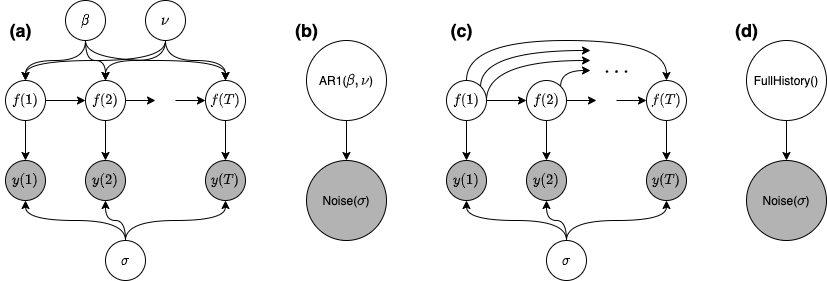
Figure 1. An STS block can simplify the graphical representation of model structure. Panel (a) displays the graphical representation of an autoregressive process, while panel (b) displays an alternate “block-based” representation of the same process. In the block-based representation, the recursive structure of the latent AR1 process has been rolled up into a single latent node. In panel (c) we display a graphical representation of a full-history latent process. This process is non-Markov and difficult to represent using typical graphical notation. However, if there exists an explicit algorithm to compute the latent process, it can again be represented in a single latent node, as displayed in panel (d).

The block notation corresponds to an explicit way of factoring of the joint density function. Let $x(t)$be the single scalar observed time series, $z(t)=(z_{1}(t),z_{2}(t),...,z_{K}(t))$ the vector of all latent time series at time $t$, and $u$ the vector of all global rvs. The usual graphical representation of a model, as in Fig. 1 panels (a) and (c), corresponds to a factoring of the joint density as

$$p(x,z,u)=p(u)\prod_{t}p(x(t)|x(t^{\prime}<t),z(t^{\prime}\leq t),u)\prod_{i}p(z_{i}(t)|z_{\lnot i}(t^{\prime}<t),u).$$

By $z(t^{\prime}<t)$ we mean the time series of rvs $z(1),z(2),...,z(t^{\prime}-1)$. The notation $z_{\lnot i}(t)$ represents the vector $(z_{1}(t),...,z_{i-1}(t),z_{i+1}(t),...)$. In this factorization, each random variable at each timestep is explicitly represented by a likelihood or prior term and corresponds to a unique node in the graphical representation. The block notation instead corresponds to the factorization

(4) $$p(x,z,u)=p(x|z,u)p(u)\prod_{i}p(z_{i}|z_{\lnot i}).$$

The temporal relationships between $z_{i}(t)$ and $z_{i}(t^{\prime})$ for $t^{\prime}<t$ are now implicit and defined within the prior terms $p(z_{i}|z_{\lnot i})$. Similarly the dynamic structure of the likelihood function is now implicit in $p(x|z,u)$ and is absent from the graphical representation. The choice to use block notation thus shifts model complexity from edge space to node space: the relationship between a pair of time series is represented by a single edge in the graph, but the definition of the multivariate random variable defining each node is more complicated.

4. STS grammar

We introduce a grammar over STS models, $G=(V,\Sigma,R,S)$, where $V=\{S,Q,p\}$, $\Sigma=\{f,\theta\}$, and the production rules $R$ are

(5a) $$S \rightarrow Q\ |\ Q+S$$

(5b) $$Q \rightarrow f(p)$$

(5c) $$p \rightarrow\theta\ |\ (S\ |\ p,...,S\ |\ p)$$

The nonterminal symbols $S$, $Q$, and $p$ represent an STS model, a block object, and a parameter-like object respectively. The symbol $Q$ is redundant but we include it because it makes a later expansion of $G$ to include changepoints easier. The terminal symbols $f$ and $\theta$ represent the generative component of a block and the parameters of the generative component of a block respectively. Production rules 5a and 5b jointly state that any STS can be extended by adding another block. Production rule 5c states that $p$ can be replaced with either an $N$-dimensional parameter vector $\theta$ or by any combination of STSs and parameter-like objects that satisfy the constraints imposed by the associated block. The dimensionality $N$ is equal to the dimensionality of the parameter space of the associated generative block component.

We can extend $G$ to express changepoint models using an augmented grammar $G^{\prime}=(V,\Sigma,R^{\prime},S)$. We define $R^{\prime}$ by replacing the second rule of $R$ with

(6) $$Q\rightarrow f(p)\ |\ C(S,f(p))\ |\ C(f(p),S).$$

The symbol $C$ is the changepoint operation; $C(x,y)$ yields a new block defined by the concatenation of $(x(1),...,x(t^{*}-1))$ and $(y(t^{*}),...,y(T))$ at a random time point $t^{*}\sim\text{DiscreteUniform}(\{2,...,T~{}-~{}1\})$. Models corresponding to sentences in $G^{\prime}$ are not generative because the existence of changepoints means that an end time must be imposed and all values of the observed time series must be known between the start and end times.

This grammar could be used to define a domain specific language (DSL). This DSL would be an interface to easily describe STS models and express relationships between latent and observed time series (for a discussion of extending the definition of STS models to include multiple observed time series, see Sec. 6).

5. Implementation

We have implemented the basic functionality of the language generated by grammar $G^{\prime}$ in the host PPL Pyro (Bingham et al., 2019). Our implementation is available online. There is a large range of dynamic behaviors expressible through the small number of operations and STS blocks that we have implemented, though our implementation is preliminary.

We have implemented a small set of fundamental blocks (corresponding to $f$ in grammars $G$ and $G^{\prime}$) that capture a range of potential time series phenomena: random walk and geometric random walk, $f(t)=f(t-1)+\varepsilon(t;\sigma)$ and $f(t)=\exp g(t)$ with $g(t)$ a random walk; first order autoregression, $f(t)=\beta f(t-1)+\varepsilon(t;\sigma)$; seasonality, $f(t)=\cos(2\pi t/\rho)$; global trend, $f(t)=a_{0}+a_{1}t$; a zero model, $f(t)=0$; and a non-Markov block, $f(t)=F[f(t-1),f(t-2),...,f(1);\varepsilon(t,\sigma)]$. The function $F$ in the non-Markov block is an arbitrary user-defined function of all past values of the latent time series $f(t)$, the current time value $t$, another time argument $s<t$ (which could be used for, e.g., constructing convolution operations); and a noise rv $\varepsilon(t;\sigma)$.

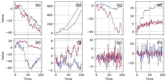
Figure 2. We display draws from prior predictive distributions for various STS models expressible using grammar $G^{\prime}$. The models are: random walk (panel a); local linear trend (panel b); semi-local linear trend (SLLT) (panel c); full-history non-Markov model (panel d); changepoint model with SLLT generative components (panel e); seasonal-global trend (panel f); stochastic volatility (panel g); and additive seasonality model with changepoint (panel h). These models can be generated using the library at https://gitlab.com/daviddewhurst/stsb.

Description	Expression
⬇ rw = Noise( RandomWalk(t1=t1), t1=t1 )
⬇ llt = Noise( RandomWalk( loc=RandomWalk(t1=t1), t1=t1, ), t1=t1 )
⬇ sllt1 = RandomWalk(loc=AR1(t1=t1), t1=t1) sllt2 = RandomWalk(loc=AR1(t1=t1), t1=t1) changepoint_sllt = Noise( changepoint_op(sllt1, sllt2), t1=t1 )
⬇ stoch_vol = Noise( Zero(t1=t1), t1=t1, scale=GeometricRandomWalk(t1=t1) )
Multiple seasonality
⬇ s = [Seasonal(t1=t1) for _ in range(4)] random_seasonal = Noise( s[0] + s[1] + changepoint_op(s[2], s[3]), t1=t1 )
Stochastic optimization
⬇ fn = lambda t, s, y, noise: torch.cat(( y.max().view((1,)), y.median() + noise.view((1,)) )).max() model_improvement = NonMarkov(t1=t1, fn=fn) optim_null_model = Noise(model_improvement, t1=t1)

Table 1. We display example implementations of various STS models described using grammar $G^{\prime}$. The current host language is Python and host PPL is Pyro. It is possible to express multi-part or full-history models, such as the multiple seasonality model or stochastic optimization null model, in very few lines of code. A minimal implementation of the language generated by $G^{\prime}$ is at https://gitlab.com/daviddewhurst/stsb.

In Table 1 we display sample Python code implementing multiple STS models expressed using the syntax of $G^{\prime}$: a latent random walk model (panel a); a local linear trend, which is a random walk with mean given by another random walk process (panel b); a nonstationary changepoint model (panel e); the stochastic volatility model represented by Eqs. 2a and 2b (panel g); a model incorporating multiple added seasonal components and a changepoint (panel h); and a full-history non-Markov model that could be used as a null model of objective function value during stochastic optimization (panel d). In Fig. 2 we display sample draws from the prior predictive distributions of each of these STS models and also display sample draws from two additional models: a semi-local linear trend, which is a random walk with mean given by an AR1 process (panel c); and a seasonal-global trend model similar to that described in Sec. 2 (panel f).

6. Future work

Future work should proceed in multiple directions.

• The grammars $G$ and $G^{\prime}$ should be formalized and a DSL should be created to implement the language generated by $G^{\prime}$.

• Ideally, the DSL would support more blocks than we have currently implemented. Useful blocks include: discrete seasonality; other non-Markov processes (e.g., self-exciting point processes, pantograph processes); discrete-valued processes; and switching processes.

• The definition of an STS to include only one observed time series and the restriction of the observed and latent time series to be one-dimensional are unnecessarily restrictive. The implementation of the DSL should allow for multiple observed time series and multivariate time series.

• We envision the DSL being used in the task of latent time series structure search: finding the DAG defined on STS block nodes that best describes the observed time series. This task will be difficult because of the large, growing search space. It may be possible to map this task onto a combinatorial multi-armed bandit problem and find an approximately optimal solution (Chen et al., 2013).

- (1)
- Bingham et al. (2019) Eli Bingham, Jonathan P Chen, Martin Jankowiak, Fritz Obermeyer, Neeraj Pradhan, Theofanis Karaletsos, Rohit Singh, Paul Szerlip, Paul Horsfall, and Noah D Goodman. 2019. Pyro: Deep universal probabilistic programming. The Journal of Machine Learning Research 20, 1 (2019), 973–978.
- Black and Scholes (1973) Fischer Black and Myron Scholes. 1973. The pricing of options and corporate liabilities. Journal of political economy 81, 3 (1973), 637–654.
- Brodersen et al. (2015) Kay H Brodersen, Fabian Gallusser, Jim Koehler, Nicolas Remy, Steven L Scott, et al. 2015. Inferring causal impact using Bayesian structural time-series models. The Annals of Applied Statistics 9, 1 (2015), 247–274.
- Chen et al. (2013) Wei Chen, Yajun Wang, and Yang Yuan. 2013. Combinatorial multi-armed bandit: General framework and applications. In International Conference on Machine Learning. 151–159.
- Choi and Varian (2012) Hyunyoung Choi and Hal Varian. 2012. Predicting the present with Google Trends. Economic record 88 (2012), 2–9.
- Dossche and Everaert (2005) Maarten Dossche and Gerdie Everaert. 2005. Measuring inflation persistence: a structural time series approach. National Bank of Belgium Working Paper 70 (2005).
- Gatheral (2006) Jim Gatheral. 2006. The volatility surface: a practitioner’s guide. Vol. 357. John Wiley & Sons.
- Moore and Burnim (2019) Dave Moore and Jacob Burnim. 2019. Structural Time Series modeling in TensorFlow Probability. https://blog.tensorflow.org/2019/03/structural-time-series-modeling-in.html
- Rodionov (2006) Sergei N Rodionov. 2006. Use of prewhitening in climate regime shift detection. Geophysical Research Letters 33, 12 (2006).
- Taylor and Letham (2018) Sean J Taylor and Benjamin Letham. 2018. Forecasting at scale. The American Statistician 72, 1 (2018), 37–45.