B₁B_s0K and B₁B_s1K strong couplings in three-point QCD sum rules

Abstract

An improved calculation of the strong coupling constants of B₁B_s0K and B₁B_s1K vertices is presented in the framework of the three-point QCD sum rules. The coupling constants are calculated, when both the $B_{s0}(B_{s1})$ and $K$ states are off-shell. Considering the $SU_{f}(3)$ symmetry, the results are compared with the existing predictions.

Key words: Strong Coupling Constant, Meson, QCD Sum Rules, $SU_{f}(3)$, Off-shell, Quark.

I Introduction

There are various applications for the strong form factors and coupling constants associated with vertices that involve mesons in the QCD, which describe the low-energy interaction among heavy mesons and light mesons, are of great importance to understand the QCD long-distance dynamics. The coupling is a fundamental parameter of the effective Lagrangian of heavy meson chiral perturbative theory (HM$\chi$PT) Cheng123 ; Burdman123 , which plays an important role in studying heavy meson physics. At high-energy physics, it is imperative to know the exact functional form of the strong form factors in meson vertices to investigate meson interactions. More accurate determination of these coupling constants plays an important role in the understanding of the interactions of the final states in the hadronic decays of the heavy mesons. The following coupling constants have been determined by different research groups:$D^{*}D^{*}\rho$MEBracco , $D^{*}D\pi$ FSNavarra ; MNielsen , $DD\rho$MChiapparini , $D^{*}D\rho$Rodrigues3 , $DDJ/\psi$ RDMatheus , $D^{*}DJ/\psi$ RRdaSilva , $D^{*}D_{s}K$, $D^{*}_{s}DK$, $D^{*}_{0}D_{s}K$, $D^{*}_{s0}DK$ SLWang , $D^{*}D^{*}P$, $D^{*}DV$, $DDV$ ZGWang , $D^{*}D^{*}\pi$ FCarvalho , $D_{s}D^{*}K$, $D_{s}^{*}DK$ ALozea , $DD\omega$ LBHolanda , $D_{s}^{*}D_{s}\phi$ Guo123 $D_{s}D_{s}V$, $D^{*}_{s}D^{*}_{s}V$ KJ ; KJ2 , $D_{1}D^{*}\pi,D_{1}D_{0}\pi,D_{1}D_{1}\pi$ Janbazi1 , $D_{s1}D^{*}K$ and $D_{s1}D^{*}K_{0}^{*}$ Janbazi2 , $D_{s}DK^{*}$ and $D_{s}D^{*}K^{*}$ Janbazi3 , $K^{*}K\pi$, $KK\phi$, $K^{*}K^{*}\phi$, $K^{*}K^{*}\rho$ Kazemi , $D_{s}^{*}D^{*}K^{*}$ and $D_{s1}D_{1}K^{*}$ Janbazi4 , and $D^{*}D^{*}_{s}K$ and $D^{*}D_{s}K$ Janbazi5 , in the framework of three-point QCD sum rules. It is very important to know the precise functional form of the form factors in these vertices and even to know how this form changes when one or the other (or both) mesons are off-shell Janbazi3 .

This review is focus on the method of three-point QCD sum rules to calculate, the strong form factors and coupling constants associated with the $B_{1}B_{s0}K$ and $B_{1}B_{s1}K$ vertices, for both the $B_{s0}(B_{s1})$ and $K$ states being off-shell. The three-point correlation function is investigated in two phenomenological and theoretical sides. In the physical or phenomenological part, the representation is in terms of hadronic degrees of freedom, which is responsible for the introduction of the form factors, decay constants, and masses. In QCD or theoretical part, which consists of two, perturbative and non-perturbative contributions (In the present work the calculations contributing the quark-quark and quark-gluon condensate diagrams are considered as non-perturbative effects), we evaluate the correlation function in quark-gluon language and in terms of QCD degrees of freedom such as, quark condensate, gluon condensate, etc, by the help of the Wilson operator product expansion(OPE). Equating two sides and applying the double Borel transformations, with respect to the momentum of the initial and final states, to suppress the contribution of the higher states and continuum, the strong form factors are estimated.

The outline of the paper is as follows. In section II, by introducing the sufficient correlation functions, we obtain QCD sum rules for the strong coupling constant of the considered $B_{1}B_{s0}K$ and $B_{1}B_{s1}K$ vertices. In obtaining the sum rules for physical quantities, both light quark-quark and light quark-gluon condensate diagrams are considered as non-perturbative contributions. In section III, the derived sum rules for the considered strong coupling constants are numerically analyzed with and without $SU_{f}(3)$ symmetry. We will obtain the numerical values for each coupling constant when both the $B_{s0}(B_{s1})$ and $K$ states are off-shell. Then taking the average of the two off-shell cases, we will obtain final numerical values for each coupling constant. In this section, we also compare our results in $SU_{f}(3)$ with the existing predictions of the other works.

II THE THREE-POINT QCD SUM RULES METHOD

To evaluate the strong coupling constants, it is necessary to know the effective Lagrangians of the interaction which, for the vertices $B_{1}B_{s0}K$ and $B_{1}B_{s1}K$, areSong12 ; 123 :

$${\cal L}_{B_{1}B_{s0}K} = -ig_{B_{1}B_{s0}K}B_{1}^{\alpha}(\partial_{\alpha}B_{s0}^{-}K^{+}-B_{s0}^{-}\partial_{\alpha}K^{+})+H.c.,$$

$${\cal L}_{B_{1}B_{s1}K} = -g_{B_{1}B_{s1}K}\epsilon^{\alpha\beta\gamma\sigma}\partial_{\alpha}B_{1\beta}(K^{+}\partial_{\gamma}B^{-}_{s1\sigma}+\partial_{\gamma}B_{{s1}\sigma}^{+}K^{-}),$$ (1)

From these Lagrangians, we can extract elements associated with the $B_{1}B_{s0}K$ and $B_{1}B_{s1}K$ momentum dependent vertices, that can be written in terms of the form factors:

$$\langle B_{1}(p^{\prime},\epsilon^{\prime})|B_{s0}(q)K(p)\rangle = g_{B_{1}B_{s0}K}(q^{2})\epsilon^{\prime}.q,$$

$$\langle B_{1}(p^{\prime},\epsilon^{\prime})|B_{s1}(q,\epsilon)K(p)\rangle = ig_{B_{1}B_{s1}K}(q^{2})\epsilon^{\alpha\beta\gamma\sigma}\epsilon^{\prime}_{\gamma}(p^{\prime})\epsilon_{\sigma}(p)p^{\prime}_{\beta}q_{\alpha},$$ (2)

where $q=p^{\prime}-p$, $g_{B_{1}B_{s0}K}(q^{2})$, and $g_{B_{1}B_{s1}K}(q^{2})$ are the strong form factor $\epsilon$ and $\epsilon^{\prime}$ are the polarization vector of the $B_{s1}$ and $B_{1}$ mesons. We study the strong coupling constants $B_{1}B_{s0}K$ and $B_{1}B_{s1}K$ vertices when both $K$ and $B_{s0}(B_{s1})$ can be off-shell. The interpolating currents $j^{K}=\bar{d}\gamma_{5}s$, $j^{B_{s0}}=\bar{s}b$, $j_{\nu}^{B_{s1}}=\bar{s}\gamma_{\nu}\gamma_{5}b$ and $j_{\mu}^{B_{1}}=\bar{d}\gamma_{\mu}\gamma_{5}b$ are interpolating currents of $K$, $B_{s0}$, $B_{s1}$, and $B_{1}$ mesons, respectively. We write the three-point correlation function associated with the $B_{1}B_{s0}K$ and $B_{1}B_{s1}K$ vertices. For the off-shell $B_{s0}(B_{s1})$ meson, Fig.1 (left), these correlation functions are given by:

$$\Pi^{B_{s0}}_{\mu}(p,p^{\prime})=i^{2}\int d^{4}xd^{4}ye^{i(p^{\prime}x-py)}\langle 0|\mathcal{T}\left\{{j^{K}}^{\dagger}(x){j^{B_{s0}}}^{\dagger}(0)j_{\mu}^{B_{1}}(y)\right\}|0\rangle,$$ (3)

$$\Pi^{B_{s1}}_{\nu\mu}(p,p^{\prime})=i^{2}\int d^{4}xd^{4}ye^{i(p^{\prime}x-py)}\langle 0|\mathcal{T}\left\{{j^{K}}^{\dagger}(x){j_{\nu}^{B_{s1}}}^{\dagger}(0)j_{\mu}^{B_{1}}(y)\right\}|0\rangle,$$ (4)

and for the off-shell $K$ meson, Fig.1 (right), these quantities are:

$$\Pi^{K}_{\mu}(p,p^{\prime})=i^{2}\int d^{4}xd^{4}ye^{i(p^{\prime}x-py)}\langle 0|\mathcal{T}\left\{{j^{B_{s0}}}^{\dagger}(x){j^{K}}^{\dagger}(0)j_{\mu}^{B_{1}}(y)\right\}|0\rangle,$$ (5)

$$\Pi^{K}_{\nu\mu}(p,p^{\prime})=i^{2}\int d^{4}xd^{4}ye^{i(p^{\prime}x-py)}\langle 0|\mathcal{T}\left\{{j_{\nu}^{B_{s1}}}^{\dagger}(x){j^{K}}^{\dagger}(0)j_{\mu}^{B_{1}}(y)\right\}|0\rangle,$$ (6)

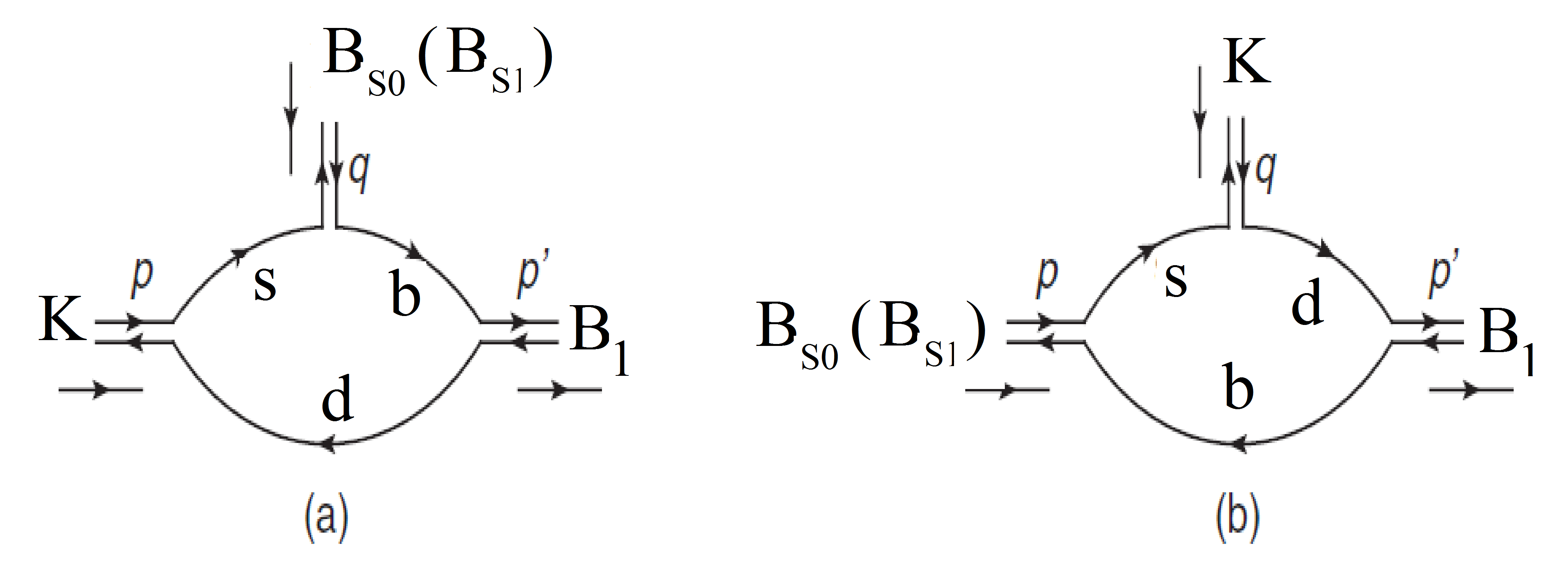
Figure 1: perturbative diagrams for off-shell $B_{s0}(B_{s1})$ (left) and off-shell $K$ (right).

Correlation function in (Eqs. (3 - 6)) in the OPE and in the phenomenological side can be written in terms of several tensor structures. We can write a sum rule to find the coefficients of each structure, leading to as many sum rules as structures. In principle, all the structures should yield the same final results but, the truncation of the OPE changes different structures in different ways. Therefore some structures lead to more stable sum rules. In the $B_{1}B_{s0}K$ vertex, we have two structures $p^{\prime}_{\mu}$ and $p_{\mu}$. Two structures give the same result for $B_{1}B_{s0}K$. We have chosen the $p^{\prime}_{\mu}$ structure. In the $B_{1}B_{s0}K$ vertex, we have only one structure $\epsilon^{\alpha\beta\mu\nu}p_{\alpha}p^{\prime}_{\beta}$.

With the help of the operator product expansion (OPE) in the Euclidean region, where $p^{2},p^{\prime 2}\to-\infty$, we calculate the QCD side of the correlation function (Eqs. (3 - 6)) containing perturbative and non-perturbative parts. In practice, only the first few condensates contribute significantly, the most important ones being the 3-dimension, $\langle\bar{d}d\rangle$, and the 5-dimension, $\langle\bar{d}\sigma_{\alpha\beta}T^{a}G^{a\alpha\beta}d\rangle$, condensates. For each invariant structure, i, we can write

$$\Pi^{(theor)}_{i}(p^{2},p^{\prime 2},q^{2}) = -\frac{1}{4\pi^{2}}\int_{(m_{d}+m_{b})^{2}}^{\infty}ds^{\prime}\int_{s_{1(2)}}^{\infty}ds\frac{\rho_{i}(s,s^{\prime},q^{2})}{(s-p^{2})(s^{\prime}-p^{\prime 2})}$$ (7)

$$+ C^{3}_{i}\langle\bar{d}d\rangle+C_{i}^{5}\langle\bar{d}\sigma_{\alpha\beta}T^{a}G^{a\alpha\beta}d\rangle+\cdots,$$

where $\rho_{i}(s,s^{\prime},q^{2})$ is spectral density, $C_{i}$ are the Wilson coefficients and $G^{a\alpha\beta}$ is the gluon field strength tensor. We take for the strange quark condensate $\langle\overline{d}d\rangle=-(0.24\pm 0.01)^{3}~{}GeV^{3}$ Ioffe and for the mixed quark-gluon condensate $\langle\bar{d}\sigma_{\alpha\beta}T^{a}G^{a\alpha\beta}d\rangle=m_{0}^{2}\langle\overline{d}d\rangle$ with $m_{0}^{2}=(0.8\pm 0.2)GeV^{2}$ Dosch .

Furthermore, we make the usual assumption that the contributions of higher resonances are well approximated by the perturbative expression

$$-\frac{1}{4\pi^{2}}\int_{s^{\prime}_{0}}^{\infty}ds^{\prime}\int_{s_{0}}^{\infty}ds\frac{\rho_{i}(s,s^{\prime},q^{2})}{(s-p^{2})(s^{\prime}-p^{\prime 2})},$$ (8)

with appropriate continuum thresholds $s_{0}$, and $s^{\prime}_{0}$.

The Cutkosky’s rule allows us to obtain the spectral densities of the correlation function for the Lorentz structures appearing in the correlation function. The leading contribution comes from the perturbative term, shown in Fig.1.

(i) For the related to the $B_{1}B_{s0}K$ vertex:

$$\rho^{B_{s0}(K)}_{B_{1}B_{s0}K} = 4N_{c}I_{0}\left[A_{2}\left(m_{2}m_{3}-km_{1}m_{2}+km_{1}m_{3}-m_{3}^{2}+\Delta-\frac{u}{2}\right)+km_{3}^{2}-m_{3}m_{1}-k\frac{\Delta}{2}\right],$$

(ii) For the $\epsilon^{\alpha\beta\mu\nu}p_{\alpha}p^{\prime}_{\beta}$ structure related to the $B_{1}B_{s1}K$ vertex:

$$\rho^{B_{s1}(K)}_{B_{1}B_{s1}K} = 4iN_{c}I_{0}\left[A_{1}\left(m_{3}-km_{1}\right)+A_{2}\left(m_{2}+m_{3}\right)+m_{3}\right],$$

The explicit expressions of the coefficients in the spectral densities entering the sum rules are given as:

$$I_{0}(s,s^{\prime},q^{2}) = \frac{1}{4\lambda^{\frac{1}{2}}(s,s^{\prime},q^{2})},$$

$$\Delta = (s+m_{3}^{2}-m_{1}^{2}),$$

$$\Delta^{\prime} = (s^{\prime}+m_{3}^{2}-m_{2}^{2}),$$

$$u = s+s^{\prime}-q^{2},$$

$$\lambda(s,s^{\prime},q^{2}) = s^{2}+s^{\prime 2}+q^{4}-2sq^{2}-2s^{\prime}q^{2}-2ss^{\prime},$$

$$A_{1} = \frac{1}{\lambda(s,s^{\prime},q^{2})}\left[2s^{\prime}\Delta-\Delta^{\prime}u\right],$$

$$A_{2} = \frac{1}{\lambda(s,s^{\prime},q^{2})}\left[2s\Delta^{\prime}-\Delta u\right],$$

Where $k=1$, $m_{1}=m_{s}$, $m_{2}=m_{b}$, $m_{3}=m_{d}$ for $B_{s0}(B_{s1})$ meson off-shell and $k=-1$, $m_{1}=m_{s}$, $m_{2}=m_{d}$, $m_{3}=m_{b}$ for $K$ meson off-shell, $N_{c}=3$ represents the color factor.

We proceed to calculate the non-perturbative contributions in the QCD side that contain the quark-quark and quark-gluon condensate. The quark-quark and quark-gluon condensate is considered when the light quark is a spectator Khodjamirian12 ; therefore only three relevant diagrams of dimension 3 and 5 remain from the non-perturbative part contributions when the $B_{s0}(B_{s1})$ meson are off-shell. These diagrams named quark-quark and quark-gluon condensate are depicted in Fig.2. For the $K$ off-shell, there is no quark-quark and quark-gluon condensate contribution.

After some straightforward calculations and applying the double Borel transformations with respect to the $p^{2}(p^{2}\rightarrow M_{1}^{2})$ and $p^{\prime 2}(p^{\prime 2}\rightarrow M_{2}^{2})$ as:

$${{B}}_{p^{2}}(M_{1}^{2})(\frac{1}{p^{2}-m^{2}_{u}})^{m}=\frac{(-1)^{m}}{\Gamma(m)}\frac{e^{-\frac{m_{u}^{2}}{M_{1}^{2}}}}{(M_{1}^{2})^{m}},$$

$${{B}}_{{p^{{}^{\prime}}}^{2}}(M_{2}^{2})(\frac{1}{{p^{{}^{\prime}}}^{2}-m^{2}_{b}})^{n}=\frac{(-1)^{n}}{\Gamma(n)}\frac{e^{-\frac{m_{b}^{2}}{M_{2}^{2}}}}{(M_{2}^{2})^{n}},$$ (9)

where $M_{1}^{2}$ and $M_{2}^{2}$ are the Borel parameters, the contributions of the quark-quark and quark-gluon condensate for the $B_{s0}(B_{s1})$ meson off-shell case, are given by:

$$\Pi_{(non-per)}^{B_{s0}(B_{s1})} = \langle\overline{d}d\rangle~{}\frac{C^{B_{s0}(B_{s1})}}{M_{1}^{4}M_{2}^{4}},$$ (10)

The explicit expressions for $C_{B_{1}B_{s0}K(B_{1}B_{s1}K)}^{B_{s0}(B_{s1})}$ associated with the $B_{1}B_{s0}K$ and $B_{1}B_{s1}K$ vertices are given in the appendix.

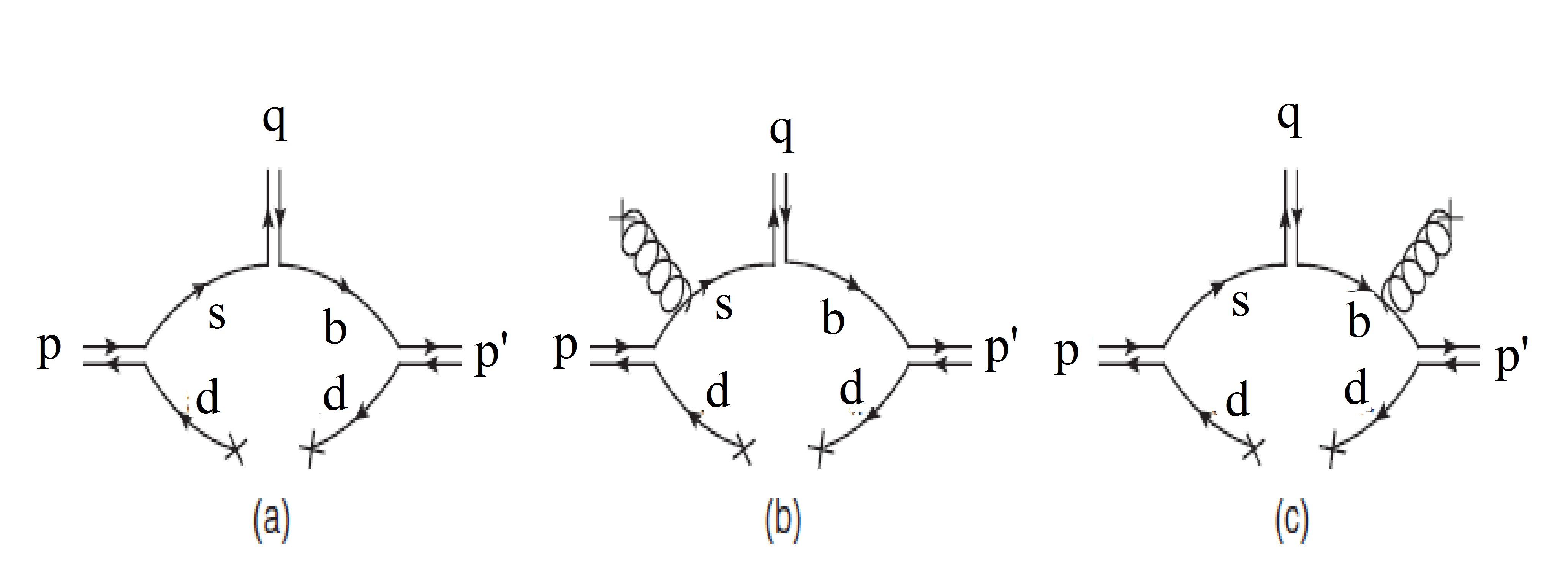
Figure 2: Contribution of the quark-quark and quark-gluon condensate for the $B_{s0}(B_{s1})$ off-shell.

The gluon-gluon condensate is considered when the heavy quark is a spectator Likhoded , and the $B_{s0}(B_{s1})$ mesons are off-shell, and there is no gluon-gluon condensate contribution. Our numerical analysis shows that the contribution of the non-perturbative part containing the quark-quark and quark-gluon diagrams is about $13\%$ and the gluon-gluon contribution is about $3\%$ of the total, and the main contribution comes from the perturbative part of the strong form factors, and we can ignore gluon-gluon contribution in our calculationGuo123 ; Janbazi3 .

The phenomenological side of the vertex function is obtained by considering the contribution of three complete sets of intermediate states with the same quantum number that should be inserted in Eqs. (3 - 6). We use the standard definitions for the decay constants $f_{M}$ ($f_{K}$, $f_{B_{s0}}$, $f_{B_{s1}}$, and $f_{B_{1}}$) and are given by:

$$\langle 0|j^{K}|K(p)\rangle = \frac{m_{K}^{2}f_{K}}{m_{s}+m_{d}},$$

$$\langle 0|j^{B_{s0}}|B_{s0}(p)\rangle = m_{B_{s0}}f_{B_{s0}},$$

$$\langle 0|j_{\nu}^{B_{s1}}|{B_{s1}}(p,\epsilon)\rangle = m_{B_{s1}}f_{B_{s1}}\epsilon_{\nu}(p),$$

$$\langle 0|j_{\mu}^{B_{1}}|{B_{1}}(p^{\prime},\epsilon^{\prime})\rangle = m_{B_{1}}f_{B_{1}}\epsilon^{\prime}_{\mu}(p^{\prime}),$$ (11)

The phenomenological part for the $p^{\prime}_{\mu}$ structure related to the $B_{1}B_{s0}K$ vertex, when $B_{s0}(K)$ is off-shell meson is:

$$\Pi^{B_{s0}(K)}_{\mu} = -g_{B_{1}B_{s0}K}^{B_{s0}(K)}(q^{2})\frac{m_{K}^{2}m_{B_{s0}}m_{B_{1}}f_{K}f_{B_{s0}}f_{B_{1}}(m_{B_{1}}^{2}+m_{K(B_{s0})}^{2}-q^{2})}{2(q^{2}-m_{B_{s0}(K)}^{2})(p^{2}-m_{K(B_{s0})}^{2})(p^{\prime 2}-m_{B_{1}}^{2})(m_{s}+m_{d})}p^{\prime}_{\mu}+h.r,$$

The phenomenological part for the $\epsilon^{\alpha\beta\mu\nu}p_{\alpha}p^{\prime}_{\beta}$ structure related to the $B_{1}B_{s1}K$ vertex, when $B_{s1}(K)$ is off-shell meson is:

$$\Pi^{B_{s1}(K)}_{\mu\nu} = -ig_{B_{1}B_{s1}K}^{B_{s1}(K)}(q^{2})\frac{m_{K}^{2}m_{B_{1}}m_{B_{s1}}f_{K}f_{B_{1}}f_{B_{s1}}}{(q^{2}-m_{B_{s1}(K)}^{2})(p^{2}-m_{K(B_{s1})}^{2})(p^{\prime 2}-m_{B_{1}}^{2})(m_{s}+m_{d})}\epsilon^{\alpha\beta\mu\nu}p_{\alpha}p^{\prime}_{\beta}+h.r,$$

In the Eqs.(II - II), h.r. represents the contributions of the higher states and continuum.

The QCD sum rules for the strong form factors are obtained after performing the Borel transformation with respect to the variables $p^{2}(B_{p^{2}}(M_{1}^{2}))$ and $p^{\prime 2}(B_{p^{\prime}}^{2}(M_{2}^{2}))$ on the physical (phenomenological) and QCD parts and equating these two representations of the correlations, we obtain the corresponding equations for the strong form factors as follows.

$\bullet$ For the $g_{B_{1}B_{s0}K}(Q^{2})$ form factors:

$$g^{B_{s0}}_{B_{1}B_{s0}K}(Q^{2}) = \frac{2(Q^{2}+m^{2}_{B_{s0}})(m_{s}+m_{d})}{m_{K}^{2}m_{B_{s0}}m_{B_{1}}f_{K}f_{B_{s0}}f_{B_{1}}(m_{B_{1}}^{2}+m_{K}^{2}+Q^{2})}~{}e^{\frac{m_{K}^{2}}{M_{1}^{2}}}e^{\frac{m_{B_{1}}^{2}}{M_{1}^{2}}}\left\{-\frac{1}{4\pi^{2}}\int^{s^{\prime}_{0}}_{(m_{b}+m_{d})^{2}}ds^{\prime}\right.$$ (14)

$$\left.\times\int^{s_{0}}_{s_{1}}ds\rho^{B_{s0}}(s,s^{\prime},Q^{2})e^{-\frac{s}{M_{1}^{2}}}e^{-\frac{s^{\prime}}{M_{2}^{2}}}+\langle d\bar{d}\rangle\frac{C_{B_{1}B_{s0}K}^{B_{s0}}}{M_{1}^{2}M_{2}^{2}}\right\},$$

$$g^{K}_{B_{1}B_{s0}K}(Q^{2}) = \frac{2(Q^{2}+m^{2}_{K})(m_{s}+m_{d})}{m_{K}^{2}m_{B_{s0}}m_{B_{1}}f_{K}f_{B_{s0}}f_{B_{1}}(m_{B_{1}}^{2}+m_{B_{s0}}^{2}+Q^{2})}~{}e^{\frac{m_{B_{s0}}^{2}}{M_{1}^{2}}}e^{\frac{m_{B_{1}}^{2}}{M_{2}^{2}}}\left\{-\frac{1}{4\pi^{2}}\int^{s^{\prime}_{0}}_{(m_{b}+m_{d})^{2}}ds^{\prime}\right.$$ (15)

$$\left.\times\int^{s_{0}}_{s_{2}}ds\rho^{K}(s,s^{\prime},Q^{2})e^{-\frac{s}{M_{1}^{2}}}e^{-\frac{s^{\prime}}{M_{2}^{2}}}\right\},$$

$\bullet$ For the $g_{B_{1}B_{s1}K}(Q^{2})$ form factors:

$$g^{B_{s1}}_{B_{1}B_{s1}K}(Q^{2}) = -i\frac{(Q^{2}+m^{2}_{B_{s1}})(m_{s}+m_{d})}{m_{K}^{2}m_{B_{1}}m_{B_{s1}}f_{K}f_{B_{1}}f_{B_{s1}}}~{}e^{\frac{m_{K}^{2}}{M_{1}^{2}}}e^{\frac{m_{B_{1}}^{2}}{M_{2}^{2}}}\left\{-\frac{1}{4\pi^{2}}\int^{s^{\prime}_{0}}_{(m_{b}+m_{d})^{2}}ds^{\prime}\right.$$ (16)

$$\left.\times\int^{s_{0}}_{s_{1}}ds\rho^{B_{s1}}(s,s^{\prime},Q^{2})e^{-\frac{s}{M_{1}^{2}}}e^{-\frac{s^{\prime}}{M_{2}^{2}}}+\langle d\bar{d}\rangle\frac{C_{B_{1}B_{s1}K}^{B_{s1}}}{M_{1}^{2}M_{2}^{2}}\right\},$$

$$g^{K}_{B_{1}B_{s1}K}(Q^{2}) = -i\frac{(Q^{2}+m^{2}_{K})(m_{s}+m_{d})}{m_{K}^{2}m_{B_{1}}m_{B_{s1}}f_{\pi}f_{B_{1}}f_{B_{s1}}}~{}e^{\frac{m_{B_{s1}}^{2}}{M_{1}^{2}}}e^{\frac{m_{B_{1}}^{2}}{M_{2}^{2}}}\left\{-\frac{1}{4\pi^{2}}\int^{s^{\prime}_{0}}_{(m_{b}+m_{d})^{2}}ds^{\prime}\right.$$ (17)

$$\left.\times\int^{s_{0}}_{s_{2}}ds\rho^{K}(s,s^{\prime},Q^{2})e^{-\frac{s}{M_{1}^{2}}}e^{-\frac{s^{\prime}}{M_{2}^{2}}}\right\},$$

where $Q^{2}=-q^{2}$, $s_{0}$ and $s^{\prime}_{0}$ are the continuum thresholds, and $s_{1}$ and $s_{2}$ are the lower limits of the integrals over $s$ as:

$$s_{1(2)}=\frac{(m_{d(b)}^{2}+q^{2}-m_{s}^{2}-s^{\prime})(m_{s}^{2}s^{\prime}-q^{2}m_{d(b)}^{2})}{(m_{s}^{2}-q^{2})(m_{d(b)}^{2}-s^{\prime})}~{}.$$ (18)

III NUMERICAL ANALYSIS

In this section, numerical analysis for the expressions of the strong coupling constant is presented. The values of masses for quarks and mesons are given in Table 1. The leptonic decay constants used in these calculations are shown in Table 2.

Table 1: The values of quark and meson masses in $\rm GeV$ PDG2012 .

$m_{s}$	$m_{b}$	$m_{K}$	$m_{B_{s0}}$	$m_{B_{s1}}$	$m_{B_{1}}$
$0.14\pm 0.01$	$4.67\pm 0.1$	$0.493$	$5.70$	$5.72$	$5.72$

Table 2: The leptonic decay constants in $\rm MeV$.

$f_{K}$fmeson	$f_{B_{1}}$Bazavov	$f_{B_{0}}$THuang	$f_{B_{s1}}$Wang
$156.1\pm 8$	$196.9\pm 8.9$	$280\pm 31$	$240\pm 20$

There are four auxiliary parameters containing the Borel mass parameters M${}_{1}^{2}$ and M${}_{2}^{2}$, and continuum thresholds $s^{K}_{0}$, $s_{0}^{B_{1}}$, $s_{0}^{B_{s0}}$ and $s_{0}^{B_{s1}}$ in Eqs.(14-17). The coupling constants and strong form factors as physical quantities should be independent of the auxiliary parameters. Howeve, the continuum thresholds are not arbitrary entirely; these are related to the energy of the first excited state. The values of the continuum thresholds are taken to be $s^{K}_{0}=(m_{K}+\delta)^{2}$, $s_{0}^{B_{s0}}=(m_{B_{s0}}+\delta^{\prime})^{2}$, $s_{0}^{B_{s1}}=(m_{B_{s1}}+\delta^{\prime})^{2}$ and $s_{0}^{B_{1}}=(m_{B_{1}}+\delta^{\prime})^{2}$. We use $0.50~{}\rm GeV^{2}\leq\delta\leq 0.90~{}\rm\rm GeV^{2}$ and $0.30~{}\rm GeV^{2}\leq\delta^{\prime}\leq 0.70~{}\rm\rm GeV^{2}$ Janbazi3 .

Our results should be almost insensitive to the Borel parameters intervals. On the other hand, the intervals of the Borel mass parameters must suppress the higher states, continuum, and contributions of the highest-order operators. In other words, the sum rule for the strong form factors must converge and the stability of our results Guo123 ; Bracco123 . This interval is called the “Borel window.” In this work, the following relations between the Borel masses $M_{1}^{2}$ and $M_{2}^{2}$ is $\frac{M_{1}^{2}}{M_{2}^{2}}=\frac{m_{K}^{2}}{m_{B_{1}}^{2}-m_{b}^{2}}$ when $B_{s0}(B_{s1})$ meson is off-shell and $M_{1}^{2}=M_{2}^{2}$ when $K$ meson is off-shell. We have illustrated the form factors of $B_{1}B_{s0}K$ and $B_{1}B_{s1}K$ vertices for $K$ off-shell respect to the Borel parameter $M_{1}^{2}$ for three values of the continuum thresholds $s^{K}_{0}$ and $s_{0}^{B_{1}}$ are shown in Figure 3. In Figure 4, we also show the pole-continuum analysis for the strong form factors $g^{K}_{B_{1}B_{s0}K}$ and $g^{K}_{B_{1}B_{s1}K}$. As it can be seen, for $M_{1}^{2}<9~{}{\rm GeV^{2}}$ the sum rule is dominated by the pole contribution for the strong form factors $g^{K}_{B_{1}B_{s0}K}$ and $g^{K}_{B_{1}B_{s1}K}$. Thus, we choose a Borel window where the pole contribution is between $20\%$ and $80\%$ of the QCDSR total contribution what we choose the interval $6~{}{\rm GeV^{2}}<M_{1}^{2}<11~{}{\rm GeV^{2}}$ for the strong form factors $g^{K}_{B_{1}B_{s0}K}$ and $g^{K}_{B_{1}B_{s1}K}$. According to the same analysis with $K$ off-shell, we choose the Borel window $8~{}{\rm GeV^{2}}<M_{1}^{2}<12~{}{\rm GeV^{2}}$ ($Q^{2}=3.0GeV^{2}$) for the strong form factors $g^{B_{s0}}_{B_{1}B_{s0}K}$ and $g^{B_{s1}}_{B_{1}B_{s1}K}$.

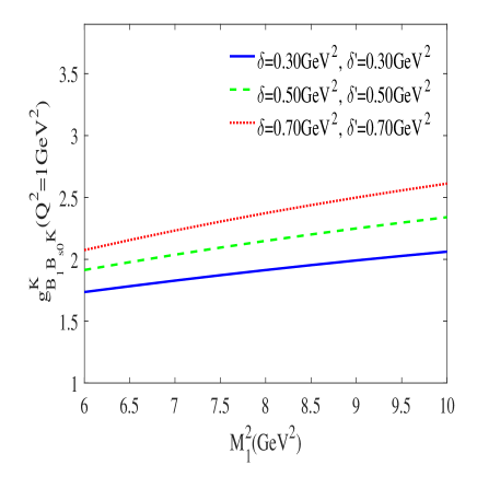
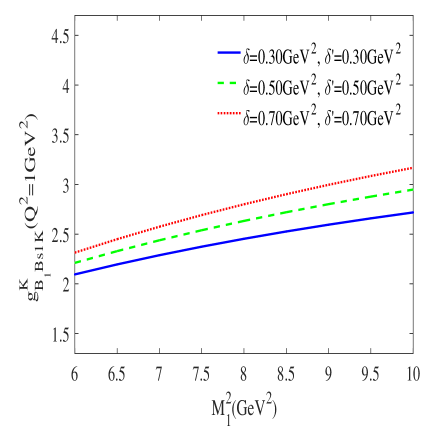
Figure 3: The strong form factors $g^{K}_{B_{1}B_{s0}K}$ (left) and $g^{K}_{B_{1}B_{s1}K}$ (right) as functions of the Borel mass parameter $M_{1}^{2}$.

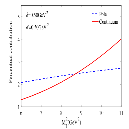
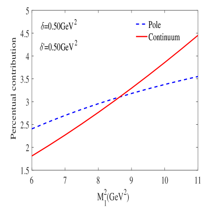
Figure 4: Pole and continuum contributions for the strong form factors $g^{K}_{B_{1}B_{s0}K}$ (left) and $g^{K}_{B_{1}B_{s1}K}$ (right) as functions of the Borel mass parameter $M_{1}^{2}$.

We have chosen the Borel mass to be $M_{1}^{2}=7~{}GeV^{2}$ and $M_{1}^{2}=9~{}GeV^{2}$ for off-shell $K$ and $B_{s0}(B_{s1})$, respectively. Having determined $M_{1}^{2}$, we calculated the $Q^{2}$ dependence of the form factors. We present the results in Fig.5 for the $g_{B_{1}B_{s0}K}$ and $g_{B_{1}B_{s1}K}$ vertices. In these figures, the small circles and boxes correspond to the form factors in the interval where the sum rule is valid. As it is seen, the form factors and their fit functions coincide together, well.

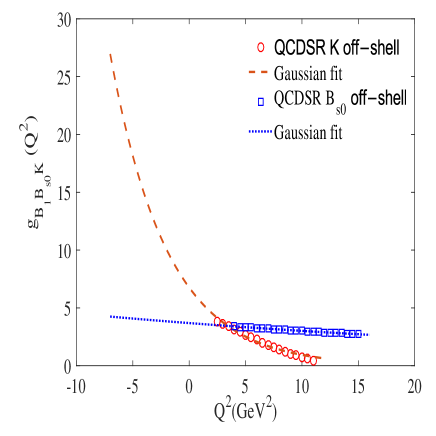
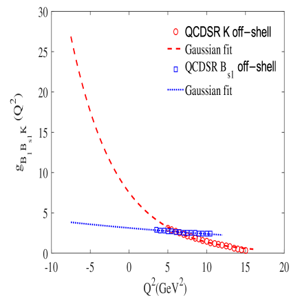
Figure 5: The strong form factors $g_{B_{1}B_{s0}K}$ and $g_{B_{1}B_{s1}K}$ on $Q^{2}$ (The boxes and circles the results of the numerical evaluation via the 3PSR for the form factors).

We discuss a difficulty inherent to the calculation of coupling constants with QCDSR. The solution of Eqs. (14-17) are numerical and restricted to a singularity-free region in the $Q^{2}$ axis, usually located in the space-like region. Therefore, in order to reach the pole position, $Q^{2}=-m_{m}^{2}$, we must fit the solution by finding a function $g(Q^{2})$, which is then extrapolated to the pole yielding the coupling constant.

The uncertainties associated with the extrapolation procedure, for each vertex is minimized by performing the calculation twice, first putting one meson and then another meson off-shell, to obtain two form factors $g^{B_{s0}(B_{s1})}$ and $g^{K}$ and equating these two functions at the respective poles.

we find that the sum rule predictions of the form factors in Eqs. (14-17) are well fitted to the following function:

$$g(Q^{2})=A~{}e^{-Q^{2}/B}.$$ (19)

The values of the parameters $A$ and $B$ are given in Table 3.

Table 3: Appeared parameters in the fit functions of the B₁B_s0K and B₁B_s1K, vertices for various $(\delta,\delta^{\prime})$, where $(\delta_{1},\delta^{\prime}_{1})=[0.30(50),0.30(0.30)],~{}(\delta_{2},\delta^{\prime}_{2})=[0.50(70),0.50(0.50)]$ and $(\delta_{3},\delta^{\prime}_{3})=[0.70(90),0.70(0.70)]~{}\rm GeV^{2}$ for $K$ [$B_{s0}(B_{s1})$] off-shell.

Form factor	$A(\delta_{1},\delta^{\prime}_{1})$	$B(\delta_{1},\delta^{\prime}_{1})$	$A(\delta_{2},\delta^{\prime}_{2})$	$B(\delta_{2},\delta^{\prime}_{2})$	$A(\delta_{3},\delta^{\prime}_{3})$	$B(\delta_{3},\delta^{\prime}_{3})$
$g^{K}_{B_{1}B_{s0}K}(Q^{2})$	6.57	5.55	6.76	5.06	7.15	4.56
$g^{B_{s0}}_{B_{1}B_{s0}K}(Q^{2})$	3.58	53.14	3.68	49.53	3.89	48.56
$g^{K}_{B_{1}B_{s1}K}(Q^{2})$	7.06	6.46	7.52	5.89	7.74	4.87
$g^{B_{s1}}_{B_{1}B_{s1}K}(Q^{2})$	2.96	37.71	3.16	37.07	3.26	35.88

We define the coupling constant as the value of the strong coupling form factor at $Q^{2}=-m_{m}^{2}$ in the Eq. (19), where $m_{m}$ is the mass of the off-shell meson. Considering the uncertainties result with the continuum threshold and uncertainties in the values of the other input parameters, we obtain the average values of the strong coupling constants shown in Table 4.

We can see that for the two cases considered here, the off- shell $K$ and $B_{s0}(B_{s1})$ meson, give compatible results for the coupling constant.

Table 4: The strong coupling constants $g_{B_{1}B_{s0}K}$ and $g_{B_{1}B_{s1}K}$ .

Coupling constant	off-shell $B_{s0}(B_{s1})$	off-shell K	Average
$g_{B_{1}B_{s0}K}$	$7.13\pm 0.52$	$7.10\pm 0.46$	$7.12\pm 0.52$
$g_{B_{1}B_{s1}K}(GeV^{-1})$	$7.65\pm 0.51$	$7.83\pm 0.34$	$7.74\pm 0.51$

In order to investigate the strong coupling constant value via the $SU_{f}(3)$ symmetry, the mass of the $s$ quark is ignored in all equations. In view of the $SU_{f}(3)$ symmetry, the values of the parameters $A$ and $B$ for the $g_{B_{1}B_{s0}K}$ and $g_{B_{1}B_{s1}K}$ vertices in $(\delta,\delta^{\prime})=[0.50(70),0.50(0.50)]~{}\rm GeV^{2}$ are given in Table 5.

Table 5: Parameters appearing in the fit functions for the $g_{B_{1}B_{s0}K}$ and $g_{B_{1}B_{s1}K}$ form factors in $SU_{f}(3)$ symmetry with $(\delta,\delta^{\prime})=[0.50(70),0.50(0.50)]~{}\rm GeV^{2}$.

Form factor	$A$	$B$	Form factor	$A$	$B$
$g^{K}_{B_{1}B_{s0}K}(Q^{2})$	4.69	5.03	$g^{B_{s0}}_{B_{1}B_{s0}K}(Q^{2})$	2.17	42.31
$g^{K}_{B_{1}B_{s1}K}(Q^{2})$	3.01	5.84	$g^{B_{s1}}_{B_{1}B_{s1}K}(Q^{2})$	1.29	34.84

In addition, considering the $SU_{f}(3)$ symmetry, we obtain the values of the coupling constants of the vertices $B_{1}B_{s0}K$ and $B_{1}B_{s1}K$, as shown in Table 6.

Table 6: The strong coupling constants $g_{B_{1}B_{s0}K}$ and $g_{B_{1}B_{s1}K}$ in $SU_{f}(3)$ symmetry.

Coupling constant	off-shell $B_{s0}(B_{s1})$	off-shell K	Average
$g_{B_{1}B_{s0}K}$	$4.71\pm 0.42$	$4.92\pm 0.36$	$4.82\pm 0.42$
$g_{B_{1}B_{s1}K}(GeV^{-1})$	$3.30\pm 0.46$	$3.14\pm 0.37$	$3.22\pm 0.45$

It is possible to compare the coupling constant values of $g_{B_{1}B_{s0}K}$ and $g_{B_{1}B_{s1}K}$ with $g_{B_{0}B_{1}\pi}$ and $g_{B_{1}B_{1}\pi}$, respectively, in the $SU_{f}(3)$ symmetry consideration. Table 7 shows a comparison between our results with the findings of others, previously calculated. From this Table, we see that our result of the coupling constants is in a fair agreement with the calculations in refs.Janbazi1 ; Zhu123 .

Table 7: Comparison of our results for strong coupling constants $g_{B_{1}B_{s0}K}$ and $g_{B_{1}B_{s1}K}$ in $SU_{f}(3)$ symmetry with the other published results.

Coupling constant	Our result	3PSR Janbazi1	LCSR Zhu123
$g_{B_{1}B_{s0}K}$	$4.82\pm 0.42$	$5.29\pm 1.40$	$4.73\pm 1.14$
$g_{B_{1}B_{s1}K}(GeV^{-1})$	$3.22\pm 0.4$	$3.57\pm 0.53$	$2.60\pm 0.60$

In summary, in this article, we analyzed the vertices $B_{1}B_{s0}K$ and $B_{1}B_{s1}K$ within the framework of the three-point QCD sum rules approach in a unified way. The strong coupling constants could give useful information about strong interactions of the strange $B_{s0}(B_{s1})$ and strange K mesons and also give useful information about the structure of the axial vector and scalar $B_{s0}(B_{s1})$ mesons.

Appendix: NON-PERTURBATIVE CONTRIBUTIONS

In this appendix, the explicit expressions of the coefficients of the quark-quark and quark-gluon condensate of the strong form factors for the vertices $B_{1}B_{s0}K$ and $B_{1}B_{s1}K$ with applying the double Borel transformations are given.

$$C_{B_{1}B_{s0}K}^{B_{s0}} = (\frac{M_{1}^{2}m_{0}^{2}m_{b}}{4}-\frac{M_{1}^{2}m_{b}^{2}m_{d}}{2}-\frac{M_{1}^{2}m_{b}m_{d}^{2}}{2}-\frac{3m_{0}^{2}M_{2}^{2}m_{s}}{4}-M_{1}^{2}M_{2}^{2}m_{s}+\frac{m_{0}^{2}m_{b}^{2}m_{s}}{4}$$

$$-\frac{M_{1}^{2}m_{b}m_{d}m_{s}}{2}+\frac{M_{1}^{2}m_{d}^{2}m_{s}}{2}-\frac{m_{b}^{2}m_{d}^{2}m_{s}}{2}-\frac{M_{1}^{2}m_{d}m_{s}^{2}}{2}-\frac{M_{2}^{2}m_{d}m_{s}^{2}}{2}+\frac{M_{2}^{2}m_{d}^{2}mu}{2}$$

$$+\frac{m_{0}^{2}m_{s}^{3}}{4}-\frac{m_{d}^{2}m_{s}^{3}}{2}+\frac{M_{1}^{2}m_{d}q^{2}}{2}-\frac{m_{0}^{2}m_{s}q^{2}}{4}+\frac{m_{d}^{2}m_{s}q^{2}}{2})\times e^{-\frac{m_{s}^{2}}{M_{1}^{2}}}~{}e^{-\frac{m_{b}^{2}}{M_{2}^{2}}},$$

$$C_{B_{1}B_{s1}K}^{B_{s1}} = i(\frac{7m_{0}^{2}M_{1}^{2}}{12}+\frac{3m_{0}^{2}M_{2}^{2}}{4}+M_{1}^{2}M_{2}^{2}-\frac{m_{0}^{2}m_{b}^{2}}{2}-\frac{M_{1}^{2}m_{b}m_{d}}{2}-M_{1}^{2}m_{d}^{2}-M_{2}^{2}m_{d}^{2}$$

$$+\frac{M_{2}^{2}m_{d}m_{s}}{2}-\frac{m_{0}^{2}m_{s}^{2}}{2}+\frac{m_{0}^{2}q^{2}}{2}-m_{d}^{2}q^{2}+m_{b}^{2}m_{d}^{2})\times e^{-\frac{m_{s}^{2}}{M_{1}^{2}}}~{}e^{-\frac{m_{b}^{2}}{M_{2}^{2}}},$$

References

(1)
T. M. Yan, H. Y. Cheng, C. Y. Cheung, G. L. Lin, Y. C. Lin and H. L. Yu, Phys. Rev. D 46, 1148 (1992) Erratum: [Phys. Rev. D 55, 5851 (1997)].
(2)
G. Burdman and J. F. Donoghue, Phys. Lett. B 280, 287 (1992).
(3)
M. E. Bracco, M. Chiapparini, F. S. Navarra, and M. Nielsen, Phys.
Lett. B 659, 559 (2008).
(4)
F. S. Navarra, M. Nielsen, M. E. Bracco, M. Chiapparini, and C. L.
Schat, Phys. Lett. B 489, 319 (2000).
(5)
F. S. Navarra, M. Nielsen, and M. E. Bracco, Phys. Rev. D 65,
037502 (2002).
(6)
M. E. Bracco, M. Chiapparini, A. Lozea, F. S. Navarra, and M.
Nielsen, Phys. Lett. B 521, 1 (2001).
(7)
B. O. Rodrigues, M. E. Bracco, M. Nielsen, and F. S. Navarra, Nucl.
Phys. A 852, 127 (2011).
(8)
R. D. Matheus, F. S. Navarra, M. Nielsen, and R. R. da Silva, Phys.
Lett. B 541, 265 (2002).
(9)
R. R. da Silva, R. D. Matheus, F. S. Navarra, and M. Nielsen, Braz.
J. Phys. 34, 236 (2004).
(10)
Z. G. Wang, and S. L. Wan, Phys. Rev. D 74, 014017 (2006).
(11)
Z. G. Wang, Nucl. Phys. A 796, 61 (2007).
(12)
F. Carvalho, F. O. Duraes, F. S. Navarra, and M. Nielsen, Phys.
Rev. C 72, 024902 (2005).
(13)
M. E. Bracco, A. J. Cerqueira, M. Chiapparini, A. Lozea, and M.
Nielsen, Phys. Lett. B 641, 286 (2006).
(14)
L. B. Holanda, R. S. Marques de Carvalho, and A. Mihara, Phys.
Lett. B 644, 232 (2007).
(15)
Yu, Guo-Liang, Zhen-Yu Li, and Zhi-Gang Wang. The European Physical Journal C 75, no. 6 (2015): 243.
(16)
R. Khosravi, and M. Janbazi, Phys. Rev. D 87, 016003 (2013).
(17)
R. Khosravi, and M. Janbazi, Phys. Rev. D 89, 016001 (2014).
(18)
M. Janbazi, N. Ghahramany, and E. Pourjafarabadi, Eur. Phys. J. C
74, 2718 (2014).
(19)
Ghahramany, N., R. Khosravi, and M. Janbazi. International Journal of Modern Physics A 27, no.05 (2012): 1250022.
(20)
Janbazi, M., and R. Khosravi. The European Physical Journal C 78.7 (2018): 606.
(21)
E. Kazemi, N. Ghahramany, Phys. Rev. D 95, 034008 (2017).
(22)
Janbazi, M., R. Khosravi, and E. Noori. Advances in High Energy Physics 2018 (2018).
(23)
Seyedhabashi, M. R., E. Kazemi, M. Janbazi, and N. Ghahramany. Nuclear
Physics A (2020): 121846.
(24)
Z. Lin and C. M. Ko, Phys. Rev. C 62, 034903 (2000).
(25)
Y. Oh, T. Song and S.H. Lee, Phys. Rev. C 63, 034901 (2001).
(27)
H.G. Dosch, M. Jamin and S. Narison, Phys. Lett. B220, 251 (1989) ; V. M. Belyaev, B. L. Ioffe, Sov. Phys. JETP, 57, 716 (1982).
(28)
P. Colangelo and A. Khodjamirian, in At the Frontier of
Particle Physics/Handbook of QCD, edited by M. Shifman
(World Scientific, Singapore, 2001), Vol. 3, pp. 1495–1576;
A.V. Radyushkin, in Proceedings of the 13th Annual HUGS
at CEBAF, Hampton, Virginia, 1998, edited by J. L. Goity
(World Scientific, Singapore, 2000), pp. 91–150.
(29)
V.V. Kiselev, A. K. Likhoded, and A. I. Onishchenko,
Nucl. Phys. B569, 473 (2000).
(30)
J. Beringer et al., Particle Data Group, Phys. Rev. D 86, 010001 (2012).
(31)
H. M. Choi, C. R. Ji, Z. Li, and H. Y. Ryu, Phys. Rev. C 92, 055203 (2015).
(32)
A. Bazavov et al., Phys. Rev. D 85, 114506 (2012).
(33)
Z. G. Wang, T. Huang, Phys. Rev. C 84, 048201 (2011).
(34)
Z.G. Wang, arXiv:0712.0118
(35)
Bracco, M. E., M. Chiapparini, F. S. Navarra, and M. Nielsen. Progress in Particle and Nuclear Physics 67, no. 4 (2012): 1019-1052.
(36)
Y.B. Dai, S.L. Zhu, Eur. Phys. J. C 6, 307–311 (1999)