Fast Magnetic Reconnection with Turbulence in High Lundquist Number Limit

Abstract

We use extensive 3D resistive MHD simulations to study how large-scale current sheets will undergo fast reconnection in the high Lundquist number $S$ limit (above $\sim 10^{4}$), when the system is subject to different externally driven turbulence levels and the self-generated turbulence produced by 3D reconnection dynamics. We find that the normalized global reconnection rate $\sim 0.01-0.13$, weakly dependent on $S$. Global reconnection with the classic inflow/outflow configurations is observed, and 3D flux ropes are hierarchically formed and ejected from reconnection regions. A statistical separation of the reconnected magnetic field lines follows a super-diffusive behavior, from which the rate is measured to be very similar to that obtained from the mixing of tracer populations. We find that the reconnection rate scales roughly linearly with the turbulence level during the peak of reconnection. This scaling is consistent with the turbulence properties produced by both the externally driven and self-generation processes. These results imply that large-scale thin current sheets tend to undergo rigorous reconnection.

1 INTRODUCTION

Fast magnetic reconnection (at a fraction of Alfvén speed $V_{A}$) is often invoked to explain energetic events such as solar/stellar flares, substorms in the magnetosphere of Earth and other planets, coronal mass ejections, sawtooth crashes in fusion plasmas, and other astrophysical systems (Priest & Forbes, 2007; Lazarian et al., 2020). During reconnection, oppositely directed magnetic field lines restructure themselves, resulting in a rapid conversion of magnetic energy into kinetic energy of bulk flows, and thermal and non-thermal particles (e.g., Drake et al., 2006).

In the limit of resistive magnetohydrodynamics (MHD) description, the classical Sweet-Parker (SP) model (Sweet, 1958; Parker, 1957) predicts a rather slow reconnection rate proportional to $S^{-1/2}$, where $S=LV_{A}/\eta$ is the Lundquist number, $\eta$ is the plasma resistivity, and $L$ is the characteristic length of the system. Many alternatives to speed up the reconnection have been investigated (Priest & Forbes, 2007; Cassak & Shay, 2012; Lin et al., 2015; Loureiro & Uzdensky, 2016). A major advance came through studies related to the resistive tearing instability (Biskamp, 1986; Loureiro et al., 2007; Bhattacharjee et al., 2009; Uzdensky et al., 2010; Huang & Bhattacharjee, 2010; Ni et al., 2012; Lin & Ni, 2018). In the high $S$ limit, it is found that, above a critical $S\sim 10^{4}$, the thin SP current sheets (CSs) in two-dimensional (2D) become violently unstable to the hierarchical formation and ejection of plasmoids (Loureiro et al., 2007), producing nearly resistivity-independent reconnection rate around $0.01\ V_{A}$.

Fast magnetic reconnection in the presence of 3D turbulence is a critically important process in space and astrophysical plasmas (Matthaeus & Lamkin, 1986; Lazarian & Vishniac, 1999; Fan et al., 2004; Kowal et al., 2009; Loureiro et al., 2009; Eyink et al., 2011; Daughton et al., 2011; Wyper & Hesse, 2015; Oishi et al., 2015; Takamoto et al., 2015; Guo et al., 2015; Huang & Bhattacharjee, 2016; Beresnyak, 2017; Kowal et al., 2017; Pisokas et al., 2018; Li et al., 2019; Ye et al., 2020), with some interesting observation support (Fu et al., 2017; He et al., 2018; Chitta & Lazarian, 2020). Broadly speaking three types of configurations have been studied in some detail, depending on what “free energy” is available. The first is on how externally driven (or decaying) turbulence affects the reconnection of a pre-existing CS(s) (e.g., Matthaeus & Lamkin, 1986; Lazarian & Vishniac, 1999; Kowal et al., 2009; Loureiro et al., 2009; Kowal et al., 2012). The 3D MHD simulations have mostly been done in the small $S$ ($\sim$ a few thousand) limit, though the externally driven turbulence with relatively large amplitude can greatly enhance the reconnection rate up to $\sim 0.1\ V_{A}$. The second is similar to the first type except that the turbulence is self-generated from instabilities associated with the pre-existing CS(s) or additional instabilities due to reconnection (e.g., Oishi et al., 2015; Huang & Bhattacharjee, 2016; Beresnyak, 2017; Kowal et al., 2017, 2020). The 3D MHD simulations in this category with $S$ up to a few times $10^{5}$ have shown that the reconnection rate is slightly slower, averaging around a few percent of $V_{A}$. Note that these two types of studies could differ in important ways because the available free energy in the second case is primarily from the initial CS only whereas in the first case both the injected turbulence and the CS contribute to the available energy for dissipation. In particular, Lazarian & Vishniac (1999, hereafter LV99) and Eyink et al. (2011, hereafter ELV11) provided the basic theoretical model on such turbulent reconnection. The third is to begin with the injected turbulence only without a pre-existing semi-global CS(s). The turbulence cascade will produce CSs at intermediate scales that could undergo reconnection. 2D MHD simulations (Dong et al., 2018; Walker et al., 2018) and 3D kinetic simulations (e.g., Makwana et al., 2015) appear to lend support to these ideas. In fact, the dual process of CS formation by turbulence cascade and the back-reaction on turbulence by the possible reconnection of such sheets have led to new models of MHD turbulence with reconnection (e.g., Loureiro & Boldyrev, 2017; Boldyrev & Loureiro, 2017). Note that the available free energy in this case is only the injected turbulence, very different from the first two types. Overall, the interplay among the externally injected turbulence vs. the self-generated turbulence, and the pre-existing CS(s) vs. the self-generated CSs makes it challenging to build a comprehensive theory. Numerical simulations tend to have a limited dynamic range to fully resolve several critical issues revealed by these theoretical models (see a recent discussion in Lazarian et al. (2020)).

In this work, we use a set of 3D compressible MHD simulations to systematically examine how the reconnection rate in the low plasma $\beta=0.1$ condition scales with the strength of turbulence as well as $S$. Our most important conclusion is that, in systems with an initial large-scale CS, the 3D reconnection rate can range between $0.01-0.1\ V_{A}$, and scales roughly linearly with the turbulent Alfvén Mach number $M_{\mathrm{A}}\sim 0.06-0.32$. The rate is weakly dependent on $S$ in the high $S$ limit. Flux ropes, as the 3D version of the 2D plasmoid instability, are frequently formed and ejected along the thin CSs. Magnetic field line tracing yields super-diffusive behavior. The turbulence is a combination of the externally driven and the self-generated fluctuations, but with a second-order structure function different from the incompressible MHD turbulence theory by Goldreich & Sridhar (1995).

2 NUMERICAL MHD MODEL

The isothermal resistive MHD equations in a periodic cube with a side length of $L=2\pi$ are solved:

$$\frac{\partial\rho}{\partial t}+\nabla\cdot(\rho\mathbf{u})=0\ ,$$ (1)

$$\frac{\partial\rho\mathbf{u}}{\partial t}+\nabla\cdot\left[\rho\mathbf{u}\mathbf{u}+(p+\frac{1}{2}\mathbf{B}^{2})\mathbf{I}-\mathbf{B}\mathbf{B}\right]=\nu\nabla^{2}\mathbf{u}+\rho\mathbf{f}_{v}\ ,$$ (2)

$$\frac{\partial\mathbf{B}}{\partial t}+\nabla\cdot(\mathbf{u}\mathbf{B}-\mathbf{B}\mathbf{u})=\eta\nabla^{2}\mathbf{B}\ .$$ (3)

$$\frac{\partial s_{i}}{\partial t}+\nabla\cdot(s_{i}\mathbf{u})=0\ ,$$ (4)

Here, $\rho$ is the mass density; $p$ is the thermal pressure; $\mathbf{u}$ is the velocity; $\mathbf{B}$ denotes the magnetic field; $t$ is time; $\nu$ is the viscosity; $\eta$ is the magnetic resistivity; $s_{i}(i=1,2)$ are the densities of the tracer populations (Yang et al., 2013); $\mathbf{f}_{v}$ is a random large-scale driving force, applied in Fourier space at $k<3.5$ (Yang et al., 2017, 2018). We have used $\nu=\eta$ in all simulations.

The initial magnetic field has a Harris configuration with two thin CSs as
$\mathbf{B}=B_{0}\left[\tanh(\frac{x-x_{1}}{w})-\tanh(\frac{x-x_{2}}{w})\right]\hat{y}-B_{0}\hat{y}$, where $B_{0}$ is the asymptotic magnetic field, $x_{1}=\pi/2$ and $x_{2}=3\pi/2$ are the initial positions of the CSs, and the parameter $w$ is set to satisfy the SP scaling of $2w/L\simeq S^{-1/2}$. Initially, the density profile is set to maintain a uniform total (thermal plus magnetic) pressure, velocity is zero, and plasma $\beta$ is about 0.1. Due to the broadening likely caused by turbulence, the CS layer during evolution is typically resolved with more than 10 cells. The externally driven turbulence is characterized by $\mathbf{f}_{v}$. When $|\mathbf{f}_{v}|=0$, the velocity is initially seeded with a random noise of amplitude $10^{-3}$. Simulation parameters are listed in Table 1, in which $N$ is grid number in one direction. $M_{\mathrm{A}}$ is Alfvén Mach number defined as $M_{\mathrm{A}}=u_{\mathrm{RMS}}/V_{A}$ with $u_{\mathrm{RMS}}$ being the root-mean-square (RMS) amplitude of the velocity at the peak reconnection, and $V_{A}$ the Alfvén speed based on the initial magnetic field $B_{0}$ and the average density. Run E only has a uniform magnetic field without any initial CSs. We use the Athena code (Gardiner & Stone, 2005; Stone et al., 2008) for simulations. Specifically, we apply the approximate Riemann solver of Harten-Lax-van Leer discontinuities (HLLD) to the calculation of the numerical fluxes, a third-order piecewise parabolic method (PPM) to the reconstruction, MUSCL-Hancock (VL) Integrator to the time integration, and the constrained transport (CT) algorithm to ensure the divergence-free state of the magnetic field.

3 NUMERICAL RESULTS

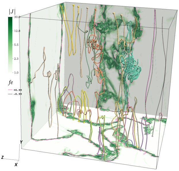
Figure 1: Spatial distribution of the total current density ($|J|$) for Run A1 at $t=2.0$. Only intersections with the three bounding planes are shown. The colored lines denote sample magnetic field lines. The pink and gray contour lines show $f_{e}=0.99$ and $-0.99$, respectively.

We find that all runs containing initial CSs will undergo global reconnection characterized by inflow/outflow patterns. Figure 1 shows that the two initially parallel thin CSs are now strongly deformed by the externally driven turbulence while undergoing 3D reconnection. The width of the CSs also demonstrates thinning and thickening at various places. A number of magnetic field lines are plotted and three typical behaviors are observed: first, field lines that are relatively smooth and arch-looking start at one side of a CS and end up at the other side of the same CS, indicating reconnection accompanied with $X-$points and large opening angles for reconnected lines; second, field lines that are far away from the CSs go through the box without reconnection; third, field lines start at one side of a CS but trace out in twisted trajectories (possibly flux ropes) and end up far away from the starting points.

Table 1: Reconnection MHD Simulations

Run	$N^{3}$	S	$M_{\mathrm{A}}$	$|\mathbf{f}_{v}|$	CSs
A1	$2048^{3}$	$2.3\times 10^{5}$	0.322	0.30	Yes
A2	$1024^{3}$	$6.3\times 10^{4}$	0.305	0.30	Yes
A3	$1024^{3}$	$1.5\times 10^{4}$	0.304	0.30	Yes
A4	$1024^{3}$	$4.8\times 10^{3}$	0.302	0.30	Yes
B1	$2048^{3}$	$2.3\times 10^{5}$	0.192	0.10	Yes
B2	$1024^{3}$	$6.3\times 10^{4}$	0.185	0.10	Yes
B3	$1024^{3}$	$1.5\times 10^{4}$	0.183	0.10	Yes
B4	$1024^{3}$	$4.8\times 10^{3}$	0.180	0.10	Yes
C1	$2048^{3}$	$2.3\times 10^{5}$	0.098	0.01	Yes
C2	$1024^{3}$	$6.3\times 10^{4}$	0.092	0.01	Yes
C3	$1024^{3}$	$1.5\times 10^{4}$	0.089	0.01	Yes
C4	$1024^{3}$	$4.8\times 10^{3}$	0.084	0.01	Yes
D1	$2048^{3}$	$2.3\times 10^{5}$	0.072	No	Yes
D2	$1024^{3}$	$6.3\times 10^{4}$	0.067	No	Yes
D3	$1024^{3}$	$1.5\times 10^{4}$	0.060	No	Yes
D4	$1024^{3}$	$4.8\times 10^{3}$	0.056	No	Yes
E	$1024^{3}$	$6.3\times 10^{4}$	0.421	0.30	No

To calculate the 3D reconnection rate, we use the method described in Daughton et al. (2014), which employs the mixing of tracer populations originating from separate sides of a CS as a proxy to identify the reconnection region and track the evolution of magnetic flux. We solve Eq. (4) using two tracer species $s_{1}$ and $s_{2}$. The initial values of $s_{1}$ and $s_{2}$ are such that: on one side of a CS, $s_{1}=-1$ and otherwise $0$, whereas on the other side of the same CS $s_{2}=1$ and otherwise $0$. As reconnection proceeds, the populations tagged by $s_{1}$ and $s_{2}$ will interpenetrate and a mixing fraction $f_{e}$ can be defined as $f_{e}=\frac{|s_{1}|-|s_{2}|}{|s_{1}|+|s_{2}|}$, which will vary continuously from $f_{e}=-1$ on one side of CS to $f_{e}=1$ to the other side of the same CS. In Figure 1, we can see that the contours of $f_{e}$ enclose the strong $|J|$ layers quite well, correlating strong mixing/reconnection with strong $|J|$. The 3D reconnection rate is calculated according to the time derivative of the unreconnected magnetic flux $\frac{\partial\Phi}{\partial t}$ within the regions with $f_{e}<-f_{c}$ or $f_{e}>f_{c}$ as $\frac{\partial\Phi}{\partial t}$ is equal to the line integral of the electric field along the surfaces of $f_{e}=-f_{c}$ or $f_{e}=f_{c}$ due to the periodic boundary condition. We have also calculated the change rate of the magnetic flux within the regions with $f_{e}\geqslant-f_{c}$ and $f_{e}\leqslant f_{c}$ and found that it is an order of magnitude smaller than $\frac{\partial\Phi}{\partial t}$. Therefore, it can be thought that the flux entering into the reconnection region is dissipated quickly. Because the boundaries that separate $f_{e}\neq\pm 1$ regions from $f_{e}=\pm 1$ regions are quite sharp, the calculated reconnection rate is insensitive if $f_{c}$ is in the range 0.9-0.995 (Daughton et al., 2014). Here, we choose $f_{c}=0.99$. The calculated reconnection rate grows first as the reconnection starts, reaching a maximum after a few Alfvén times, then gradually decreasing.

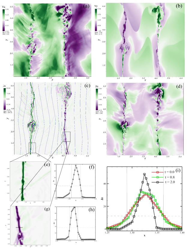
Figure 2: Spatial distributions of a 2D $x-y$ slice at $z=1.2$ of the velocity components $V_{x}$ (panel a) and $V_{y}$ (panel b), the current density $J_{z}$ component along with the (blue lines) magnetic field lines projected into the $x-y$ plane (panel c), and the magnetic field component $B_{z}$ (panel d) for Run A1 at $t=2.0$. Panels e and g zoom in around two strong $|J_{z}|$ regions; panels f and h show the one-dimensional (1D) distribution of $|J_{z}|$ along the black lines in panels e and g; and panel i shows the 1D distribution of $|J_{z}|$ at different times, with the black line being the same as that in panel f. The cell size is $\sim 0.003$ in this run.

To further demonstrate global reconnection in our simulations, we show in Figure 2 that the classic $X-$point inflow/outflow configuration is approximately preserved in the turbulent reconnection. The plasma originating from separate sides of the CSs flows into the reconnection region with an inflow speed of $\sim 0.15V_{A}$, meanwhile the outflows along the CSs appear to reach values of $\sim\pm V_{A}$ (from which the global reconnection rate could also be estimated to be $\sim 0.15$ for Run A1). There seems to be one major reconnection $X-$point in the left CS near $y=0$ whereas plasmoid-like chains with large $|J_{z}|$ and $|B_{z}|$ are visible in the right CS. In addition, in the left CS between $y=0$ and $2$, the strong shear in $|\Delta V_{y}|/(|B_{y}|/\sqrt{\rho})>2$ might indicate the excitation of Kelvin-Helmholtz instability (Miura & Pritchett, 1982; Kowal et al., 2020).

To understand the current sheet structure in more detail, we evaluate the current sheet width for Run A1 at different times, which is defined when $|J_{z}|$ comes to $e^{-1}$ of its maximum. In panels f and h of Figure 2, we give two examples of the current sheet width at $t=2.0$, in which the horizontal dashed lines cut through the $|J_{z}|$ structure, and two vertical solid lines mark the current sheet width, which is about 0.033 and is resolved by about 10 cells. In panel i, we show the evolution of the current sheet width. It starts with a width about 0.073 (resolved by about 24 cells), and undergoes a thinning process but it remains broader than that predicted by the SP scaling, presumably due to the turbulence. Overall, the current sheet width is adequately resolved numerically.

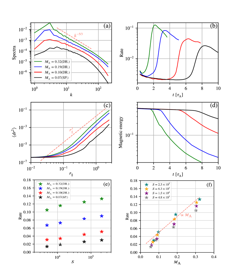
Figure 3: Power spectra of kinetic energy (panel a), global reconnection rate (panel b), diffusion of reconnecting magnetic field lines (panel c), and magnetic energy evolution (panel d) for different levels of turbulence driving for Run A1, B1, C1, and D1, global reconnection rates as a function of the Lundquist number $S$ for different values of the Alfvén Mach number $M_{\mathrm{A}}$ (panel e) and as a function of $M_{\mathrm{A}}$ for different $S$ (panel f). Quantities in panels (a) and (c) are calculated at the time when the global reconnection rate shown in panel (b) reaches its respective maximum.

We now discuss the turbulence properties in further detail. Panel (a) of Figure 3 shows that the power spectra of kinetic energy displays a $\sim-5/3$ power law for different Runs A1 - D1, although the weaker turbulence runs seem to show slightly flatter spectra. Because the plasma $\beta\sim 0.1$, the turbulence is sub-Alfvénic but becoming transonic for $M_{\mathrm{A}}\sim 0.3$ (Run A1). The rate for the strongest external driving turbulence (Run A1) is about $0.128\ V_{A}$, which is consistent with the estimate measured from inflow and outflow speeds shown in Figure 2. The rate for spontaneous turbulent reconnection (Run D1) is about $0.025\ V_{A}$, which is basically consistent with the results by Oishi et al. (2015); Beresnyak (2017); Kowal et al. (2017). In addition, the sharp rise of the rates corresponds well with the rapid decrease of the total magnetic energy within the simulation box, indicating that the fast reconnection has dissipated a significant fraction of the available magnetic energy (by $\sim 50\%$ to nearly $100\%$).

To see the connection between the reconnection rates and the diffusion of turbulent magnetic fields, we measure the separation $dr$ of numerous pairs of field lines as a function of $r_{\parallel}$ (the distance along the field lines) like Beresnyak (2013). These pairs start at random positions within the reconnection regions with $|f_{e}|<1$. Panel (c) of Figure 3 shows the relationship between $\langle dr^{2}\rangle$ and $r_{\parallel}$ in which $10^{5}$ field line pairs are used for statistical averaging. A stochastic separation of magnetic field lines follows a super-diffusion behavior. As the reconnection proceeds, $\langle dr^{2}\rangle$ rises. At the turbulence injection scale, $r_{\parallel}\sim 3$, we can calculate the field line separation rate as $\langle dr^{2}\rangle^{0.5}/r_{\parallel}$, similar to Lazarian & Vishniac (1999) and Eyink et al. (2011). The rates for Run A1, B1, C1, and D1 are 0.123, 0.093, 0.036, 0.023, respectively, which are similar to the maximum of the global reconnection rates obtained from the mixing of traced populations as shown in panel (b). =However, when $r_{\parallel}>0.1$, the standard deviation of the averaged rates for Run A1, B1, C1, and D1 increases to be the same order of magnitude as the average value $\langle dr^{2}\rangle$.

Applying these analyses to all the runs (except Run E) listed in Table 1, we summarize the dependence of 3D reconnection rates (taken at the peak of their evolution) on $S$ and $M_{\mathrm{A}}$. As shown by Panel (e) of Figure 3, the reconnection rate shows a rather weak increasing trend as $S$ increases. Even higher $S$ values are needed to see if the reconnection rate becomes weakly dependent on $S$. Note that the variation of reconnection rates for a given $M_{\mathrm{A}}$ is within $\sim 50\%$ as $S$ goes from $4.8\times 10^{3}$ to $2.3\times 10^{5}$. Assuming that the reconnection rate stays below $V_{A}$ for very large $S$, it is reasonable to expect that the dependence of the reconnection rate on $S$ should be rather weak. Consequently, we conclude that the reconnection rate is weakly dependent on $S$ when $S$ is large.

The reconnection rate, however, does show a clear dependence on the level of turbulence. Panel (f) of Figure 3 shows that the rate scales roughly linearly with the turbulent $M_{\mathrm{A}}$. This slope is obtained by mostly using points from simulation Runs A-C with the same $S$. The weak dependence on $S$ can also be seen. In addition, it seems that the “spontaneous” Runs D cannot be regarded as simply an extrapolation to zero $f_{v}$, as their reconnection rates are a bit lower than the extrapolation from Runs A-C. We suggest that this is due to a fundamental change of the turbulence properties between Runs A and Runs D. For Runs A, the turbulence mostly experiences forward cascades, whereas for Runs D, the fluctuations are first injected at the CS width scales, then undergoing both forward and inverse cascades (Bowers & Li, 2007).

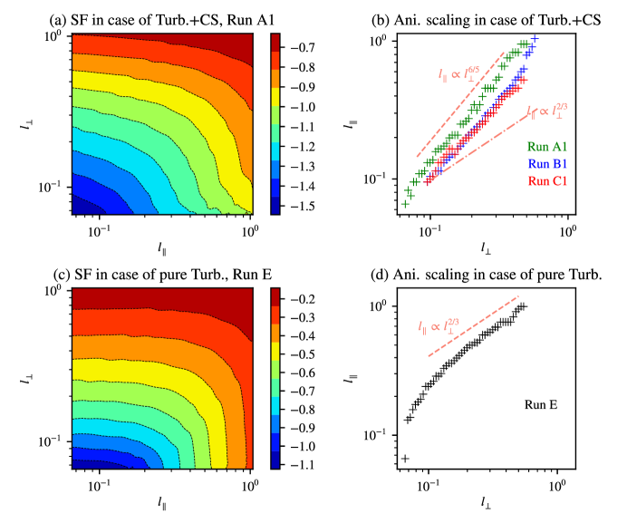
Figure 4: Second-order structure functions (SF) of velocity from the fully developed turbulence with the large-scale CSs (panel a) and without the initial large-scale CSs (pure turbulence, panel c); Panels (b) and (d): relationships between semimajor axis $l_{\parallel}$ and semiminor axis $l_{\perp}$ of contours in panels (a) and (c), which measure the scale dependency of turbulent eddy anisotropy.

To investigate the turbulence properties in more detail, we analyze the anisotropy of the turbulence using Run A1, B1, and C1. We have calculated the second-order structure functions (SF) of velocity in terms of parallel $l_{\parallel}$ and perpendicular displacement $l_{\perp}$ with respect to the local magnetic field reference frame and the correspondence between $l_{\parallel}$ and $l_{\perp}$ by equating SF values in parallel and perpendicular directions (Beresnyak, 2017; Kowal et al., 2017). The results are shown in Figures 4(a) and (b). To facilitate a comparison, the results for the fully developed turbulence without the initial large-scale CSs (Run E) are also presented in Figures 4(c) and (d).

The resulting SFs clearly display that turbulent eddies are elongated along the local magnetic field direction for Run A1. For pure turbulence Run E, eddies become increasingly more anisotropic at smaller scales, basically conforming to the Goldreich $\&$ Sridhar prediction (Goldreich & Sridhar, 1995). Comparing the properties from Run A1 and E, however, we see that the anisotropy in Run A1 is weaker than that in Run E, showing a power-law scaling with $l_{\parallel}\propto l_{\perp}^{6/5}$ for all the scales captured in the simulation. Although both Run B1 and Run C1 have smaller Alfvén Mach numbers than Run A1, the anisotropy in them displays a power-law scaling closer to $l_{\parallel}\propto l_{\perp}^{6/5}$ than $l_{\parallel}\propto l_{\perp}^{2/3}$. This may be owing to the fact that how the turbulence is produced in our current models is different from the traditional Goldreich & Sridhar (1995)’s model, as discussed in the next section.

4 DISCUSSION

The results presented here extend the previous studies in 3D turbulent MHD reconnection by systematically examining the previous unexplored parameter space in both $S$ and $M_{\mathrm{A}}$. On the one hand, we find good consistency with the previous results in the low $S$ and/or low $M_{\mathrm{A}}$ regimes such as the reconnection rates ranging between $0.01-0.1V_{A}$. On the other hand, we find two new conclusions: one is that the reconnection rate is weakly dependent on $S$ in the large $S$ limit and the other is that the reconnection rate scales roughly linearly with the turbulent $M_{\mathrm{A}}$. The weak dependence on $S$ is consistent with both the turbulent reconnection model (Lazarian & Vishniac, 1999) and plasmoid-mediated reconnection model (Loureiro et al., 2007; Bhattacharjee et al., 2009; Uzdensky et al., 2010; Huang & Bhattacharjee, 2010).

The new, linear scaling relationship we find between the reconnection rate and the strength of turbulence is different from the $M_{\mathrm{A}}^{2}$ scaling given in Lazarian & Vishniac (1999). Our turbulence properties are also different from Goldreich & Sridhar (1995). Using the anisotropy scaling from our simulations, we can derive our new reconnection rate dependence on $M_{\mathrm{A}}$ in the context of the turbulent reconnection theory Lazarian & Vishniac (1999); Eyink et al. (2011). From the constant energy transfer rate of $\dot{\xi}\sim\frac{v_{k}^{2}}{\tau_{nl}}\sim v_{k}^{4}\frac{k_{\perp}^{2}}{k_{\|}V_{\mathrm{A}}}$ (Lazarian & Vishniac, 1999) and the simulation result of $k_{\|}\sim k_{\perp}^{6/5}$, we can get that $v_{k_{\perp l}}\sim v_{k_{\perp L}}k_{\perp L}^{1/5}/k_{\perp l}^{1/5}$, with $L$ being energy injection scale, $l$ being inertial scale, $k_{\perp L}\sim 1/L$, $k_{\perp l}\sim 1/l$, and $v_{k_{\perp L}}$ as well as $v_{k_{\perp l}}$ being the corresponding perpendicular fluctuating velocities. As a pair of field lines with an initial distance of $l_{\perp}^{(0)}$ separate at the rate $\frac{d}{ds}l_{\perp}\sim\frac{\delta b_{\perp l}}{B_{0}}\sim\frac{\delta v_{\perp l}}{V_{A}}$ (Eyink et al., 2011), one finds that $\frac{d}{ds}l_{\perp}\sim\frac{v_{k_{\perp L}}k_{\perp L}^{1/5}}{k_{\perp l}^{1/5}V_{\mathrm{A}}}$, that is $l_{\perp}\sim M_{\mathrm{A}}^{5/4}k_{\perp L}^{1/4}s^{5/4}$ with $M_{\mathrm{A}}=v_{k_{\perp L}}/V_{\mathrm{A}}$. We can estimate rate by $l_{\perp}/s\sim M_{A}^{5/4}$. Given that the inertial range is limited and the turbulence is not steady, our numerical result of the rate $\propto M_{\mathrm{A}}$ is approximately consistent with this relationship.

The nature of turbulence from Runs A to D likely undergoes significant changes. The turbulence in our simulations come from both the external driven origin as well as the self-generated origin. In Run A1, the reconnection rate is high and the flow from the 3D reconnection is quite significant (the outflow speeds reaching $V_{A}$ as shown in Figure 2). Both the presence of large-scale reconnection CSs and the flows associated with reconnection are affecting the turbulence. In fact, according to Table 1, comparing Run A2 and Run E where the external driving $f_{v}$ is the same (and the same numerical resolution), the turbulent $M_{\mathrm{A}}$ is actually larger in the pure turbulence run ($0.421$) than that in the reconnection run ($0.305$). Because the self-generated turbulence likely undergoes both forward and inverse cascades, its spectral properties and anisotropy will not follow the Goldreich $\&$ Sridhar theory, especially when the turbulence properties are examined at just a few Alfvén times. In addition, our simulations are in the low $\beta$ situation (initially at $0.1$) with an aim to model the solar coronal environment whereas most previous simulations have mostly explored the higher $\beta$ limit (Oishi et al., 2015; Beresnyak, 2017; Kowal et al., 2017). According to the results of Kowal et al. (2017), the anisotropy degree and scaling depend on the plasma $\beta$ and larger $\beta$ conditions tend to yield scalings closer to the Goldreich $\&$ Sridhar theory.

The self-generated turbulence/fluctuations likely have several origins. The first is from the resistive tearing instabilities on relatively smaller scales of CS thickness; second is from the Kelvin-Helmholtz instability in the localized outflow regions, again on CS thickness scales; third is from the “collisions” of outflows (see $y\sim 2-3$ in Fig. 2). Although these processes can all in principle produce turbulence, our simulations probably do not have enough spatial separation to see the development of all these turbulence. Overall, the third process likely contribute the most to the self-generated turbulence.

Because the “spontaneous” Runs can already produce $M_{\mathrm{A}}\geq 0.06$ with a reconnection rate $\sim 0.01V_{A}$, this implies that, in space and astrophysical systems and to the extent that periodic boundary conditions can be approximately true, large-scale current sheets with high $S$ will tend to be destroyed within several Alfvén transient times of the system.

References

- Beresnyak (2013) Beresnyak, A. 2013, ApJ, 767, L39
- Beresnyak (2017) —. 2017, ApJ, 834, 47
- Bhattacharjee et al. (2009) Bhattacharjee, A., Huang, Y.-M., Yang, H., & Rogers, B. 2009, Physics of Plasmas, 16, 112102
- Biskamp (1986) Biskamp, D. 1986, Physics of Fluids, 29, 1520
- Boldyrev & Loureiro (2017) Boldyrev, S. & Loureiro, N. F. 2017, ApJ, 844, 125
- Bowers & Li (2007) Bowers, K. & Li, H. 2007, Phys. Rev. Lett., 98, 035002
- Cassak & Shay (2012) Cassak, P. A. & Shay, M. A. 2012, Space Sci. Rev., 172, 283
- Chitta & Lazarian (2020) Chitta, L. P. & Lazarian, A. 2020, ApJ, 890, L2
- Daughton et al. (2014) Daughton, W., Nakamura, T. K. M., Karimabadi, H., Roytershteyn, V., & Loring, B. 2014, Physics of Plasmas, 21, 052307
- Daughton et al. (2011) Daughton, W., Roytershteyn, V., Karimabadi, H., Yin, L., Albright, B. J., Bergen, B., & Bowers, K. J. 2011, Nature Physics, 7, 539
- Dong et al. (2018) Dong, C., Wang, L., Huang, Y.-M., Comisso, L., & Bhattacharjee, A. 2018, Phys. Rev. Lett., 121, 165101
- Drake et al. (2006) Drake, J. F., Swisdak, M., Che, H., & Shay, M. A. 2006, Nature, 443, 553
- Eyink et al. (2011) Eyink, G. L., Lazarian, A., & Vishniac, E. T. 2011, ApJ, 743, 51
- Fan et al. (2004) Fan, Q.-L., Feng, X.-S., & Xiang, C.-Q. 2004, Physics of Plasmas, 11, 5605
- Fu et al. (2017) Fu, H. S., Vaivads, A., Khotyaintsev, Y. V., André, M., Cao, J. B., Olshevsky, V., Eastwood, J. P., & Retinò, A. 2017, Geophys. Res. Lett., 44, 37
- Gardiner & Stone (2005) Gardiner, T. A. & Stone, J. M. 2005, Journal of Computational Physics, 205, 509
- Goldreich & Sridhar (1995) Goldreich, P. & Sridhar, S. 1995, ApJ, 438, 763
- Guo et al. (2015) Guo, F., Liu, Y.-H., Daughton, W., & Li, H. 2015, ApJ, 806, 167
- He et al. (2018) He, J., Zhu, X., Chen, Y., Salem, C., Stevens, M., Li, H., Ruan, W., Zhang, L., & Tu, C. 2018, ApJ, 856, 148
- Huang & Bhattacharjee (2010) Huang, Y.-M. & Bhattacharjee, A. 2010, Physics of Plasmas, 17, 062104
- Huang & Bhattacharjee (2016) —. 2016, ApJ, 818, 20
- Kowal et al. (2017) Kowal, G., Falceta-Gonçalves, D. A., Lazarian, A., & Vishniac, E. T. 2017, ApJ, 838, 91
- Kowal et al. (2020) Kowal, G., Falceta-Gonçalves, D. A., Lazarian, A., & Vishniac, E. T. 2020, ApJ, 892, 50
- Kowal et al. (2009) Kowal, G., Lazarian, A., Vishniac, E. T., & Otmianowska-Mazur, K. 2009, ApJ, 700, 63
- Kowal et al. (2012) —. 2012, Nonlinear Processes in Geophysics, 19, 297
- Lazarian et al. (2020) Lazarian, A., Eyink, G. L., Jafari, A., Kowal, G., Li, H., Xu, S., & Vishniac, E. T. 2020, Physics of Plasmas, 27, 012305
- Lazarian & Vishniac (1999) Lazarian, A. & Vishniac, E. T. 1999, ApJ, 517, 700
- Li et al. (2019) Li, X., Guo, F., Li, H., Stanier, A., & Kilian, P. 2019, ApJ, 884, 118
- Lin et al. (2015) Lin, J., Murphy, N. A., Shen, C., Raymond, J. C., Reeves, K. K., Zhong, J., Wu, N., & Li, Y. 2015, Space Sci. Rev., 194, 237
- Lin & Ni (2018) Lin, J. & Ni, L. 2018, in Electric Currents in Geospace and Beyond, ed. A. Keiling, O. Marghitu, & M. Wheatland, Vol. 235, 239–255
- Loureiro & Boldyrev (2017) Loureiro, N. F. & Boldyrev, S. 2017, Phys. Rev. Lett., 118, 245101
- Loureiro et al. (2007) Loureiro, N. F., Schekochihin, A. A., & Cowley, S. C. 2007, Physics of Plasmas, 14, 100703
- Loureiro & Uzdensky (2016) Loureiro, N. F. & Uzdensky, D. A. 2016, Plasma Physics and Controlled Fusion, 58, 014021
- Loureiro et al. (2009) Loureiro, N. F., Uzdensky, D. A., Schekochihin, A. A., Cowley, S. C., & Yousef, T. A. 2009, MNRAS, 399, L146
- Makwana et al. (2015) Makwana, K. D., Zhdankin, V., Li, H., Daughton, W., & Cattaneo, F. 2015, Physics of Plasmas, 22, 042902
- Matthaeus & Lamkin (1986) Matthaeus, W. H. & Lamkin, S. L. 1986, Physics of Fluids, 29, 2513
- Miura & Pritchett (1982) Miura, A. & Pritchett, P. L. 1982, J. Geophys. Res., 87, 7431
- Ni et al. (2012) Ni, L., Ziegler, U., Huang, Y.-M., Lin, J., & Mei, Z. 2012, Physics of Plasmas, 19, 072902
- Oishi et al. (2015) Oishi, J. S., Mac Low, M.-M., Collins, D. C., & Tamura, M. 2015, ApJ, 806, L12
- Parker (1957) Parker, E. N. 1957, J. Geophys. Res., 62, 509
- Pisokas et al. (2018) Pisokas, T., Vlahos, L., & Isliker, H. 2018, ApJ, 852, 64
- Priest & Forbes (2007) Priest, E. & Forbes, T. 2007, Magnetic Reconnection
- Stone et al. (2008) Stone, J. M., Gardiner, T. A., Teuben, P., Hawley, J. F., & Simon, J. B. 2008, ApJS, 178, 137
- Sweet (1958) Sweet, P. A. 1958, in IAU Symposium, Vol. 6, Electromagnetic Phenomena in Cosmical Physics, ed. B. Lehnert, 123
- Takamoto et al. (2015) Takamoto, M., Inoue, T., & Lazarian, A. 2015, ApJ, 815, 16
- Uzdensky et al. (2010) Uzdensky, D. A., Loureiro, N. F., & Schekochihin, A. A. 2010, Physical Review Letters, 105, 235002
- Walker et al. (2018) Walker, J., Boldyrev, S., & Loureiro, N. F. 2018, Phys. Rev. E, 98, 033209
- Wyper & Hesse (2015) Wyper, P. F. & Hesse, M. 2015, Physics of Plasmas, 22, 042117
- Yang et al. (2013) Yang, L., He, J., Peter, H., Tu, C., Chen, W., Zhang, L., Marsch, E., Wang, L., Feng, X., & Yan, L. 2013, ApJ, 770, 6
- Yang et al. (2017) Yang, L., He, J., Tu, C., Li, S., Zhang, L., Marsch, E., Wang, L., Wang, X., & Feng, X. 2017, ApJ, 836, 69
- Yang et al. (2018) Yang, L., Zhang, L., He, J., Tu, C., Li, S., Wang, X., & Wang, L. 2018, ApJ, 866, 1
- Ye et al. (2020) Ye, J., Cai, Q., Shen, C., Raymond, J. C., Lin, J., Roussev, I. I., & Mei, Z. 2020, ApJ, 897, 64