Dynamic dimensional reduction in the Abelian sandpile

Abstract.

We prove the dimensional reduction conjecture of Fey, Levine, and Peres (2010) on the hypercube. The proof shows that dimensional reduction, symmetry, and regularity of the Abelian sandpile persist during the parallel toppling process. This stronger result verifies empirical observations first documented by Liu, Kaplan, and Gray (1990).

1. Introduction

1.1. Overview

Let $\mathcal{C}_{N}^{(d)}$ be a hypercube of side length $N$ centered at the origin in the $d$-dimensional integer lattice $\mathbb{Z}^{d}$. A sandpile is a function $s:\mathcal{C}_{N}^{(d)}\to\mathbb{Z}$. Start with $2d$ chips in the hypercube, $s=s_{0}^{(d)}\equiv 2d$, then iterate the following rule: every site with at least $2d$ chips on it becomes unstable and topples in parallel, simultaneously giving one chip to each of its $2d$ neighbors. If a boundary site topples, it loses chips over the edge. Eventually every site is stable and the process stops, yielding a sequence of sandpiles over time $\{s_{t}^{(d)}\}_{t\geq 0}$ [BTW87, Dha90, HLM⁺08, LP10, LP17, Jár18, Kli18].

Simulations suggest an exact relationship between these sandpiles across size $N$, time $t$, and dimension $d$ — see Figures 1 and 2. Specifically, it appears that smaller sandpiles are embedded in larger sandpiles of the same dimension at certain times. Moreover, central cross sections of $d$-dimensional sandpiles coincide almost exactly with $(d-1)$-dimensional sandpiles for all time.

In this article, we provide a rigorous proof of these observations, self-similarity and dimensional reduction, via a simultaneous induction on all parameters: size, time, and dimension. Along the way, we develop new techniques for analyzing the parallel toppling process which may be of independent interest.

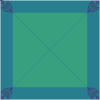
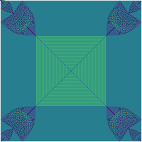
Figure 1. $s_{t}^{(2)}$ for $t=(25)^{2},(50)^{2},(100)^{2},\infty$, where $N=200$ and $s_{0}\equiv 4$. Sites with $0,\ldots,7$ chips are represented by different colors.

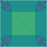
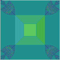
Figure 2. $s_{t}^{(3)}(\cdot,\cdot,\mbox{offset})$ for $\mbox{offset}=0,20,40,60$, where $t=(50)^{2}$, $N=200$, and $s_{0}\equiv 6$. Sites with $0,\ldots,11$ chips are represented by different colors and ‘offset’ is distance to the center of $\mathcal{C}_{N}^{(3)}$.

Dimensional reduction in sandpiles has been known experimentally since at least the work of Liu, Kaplan, and Gray in 1990 [LKG90]. In 2010, Fey, Levine, and Peres formulated an approximate dimensional reduction conjecture in the context of the single-source sandpile [FLP10] — this was later highlighted in a survey by Levine and Propp [LP10]. Soon after, Pegden and Smart, in a breakthrough, used the theory of viscosity solutions to show that the large-scale patterns which appear in sandpiles can be described by a limiting sandpile PDE [PS13]. This led to a series of works, joint with Levine, which provide a remarkable understanding of sandpiles on $\mathbb{Z}^{2}$ [LPS17, LPS16, PS20].

The structure of the sandpile PDE reveals that on torus-like domains one can construct limit sandpiles in $\mathbb{R}^{d}$ from those in $\mathbb{R}^{d-1}$. This is also possible for certain random sandpiles [BR21]. However, it has remained completely open to prove (or disprove) dimensional reduction for any natural example, on either the lattice or the continuum, till now.

Our proof in this paper leverages discrete techniques to establish dimensional reduction on the hypercube when $s_{0}\equiv 2d$. The main insight is recognizing that the parallel toppling process together with strong induction can be used to control the sandpile as it stabilizes. We identify a delicate interplay between the initial condition and the symmetry of the hypercube which forces the ‘flow’ of parallel toppling to preserve dimensional reduction. In fact, we do not know how to prove dimensional reduction for only the terminal sandpile. Our proof involves no technology from viscosity solutions nor knowledge of the sandpile PDE.

A key step in the proof is the application of certain discrete derivative bounds — Corollary 2.2 and Lemma 2.5 below. The strength of these bounds deteriorates as the initial condition grows and it is only when $s_{0}\equiv 2d$ that they are strong enough to ensure dimensional reduction.

This dependence on the initial condition provides some explanation for what occurs in the single-source version. Fey-Levine-Peres conjectured that when the initial condition is $(2d-2)+n\delta_{0}$ dimensional reduction occurs after carving out a region near the origin. This is likely because our derivative bound (which, in the single-source version, has a flipped dependence on the constant background) does not hold near the origin, but only holds away from it. Proving this remains open, but we believe the methods in this paper extend to this and other initial data.

In fact, the result in this paper appears to be a special case of a more general one which we cannot yet prove: dimensional reduction occurs for any uniform initial condition in high enough dimensions. Specifically, for integer $k\geq 0$, when $s_{0}\equiv 2d+k$, above a critical dimension, $d>d_{0}:=k+1$, exact dimensional reduction, modulo $(d_{0}-1)$-dimensional defects, appears to persist throughout the parallel toppling process. We show that when $d=d_{0}$, dimensional reduction fails to occur, providing one explanation for why $(d_{0}-1)$-dimensional defects appear — see Table 1.

1.2. Main Result

Our proof begins with the odometer $v_{t}$, which encodes the number of topples at each site over time. Let $v_{0}:\mathcal{C}_{N}^{(d)}\to\mathbb{Z}^{+}$ be the initial odometer $v_{0}\equiv 0$; then, recursively,

(1) $$v_{t+1} =v_{t}+1\{s_{t}\geq 2d\},$$

(2) $$s_{t+1} =s_{t}+\Delta(v_{t+1}-v_{t}),$$

where $\Delta$ is the graph Laplacian on $\mathcal{C}_{N}^{(d)}$ with dissipating boundary conditions. Dependence on $d$ and $N$ is indicated by writing $v_{t}^{(d,N)}$ and $s_{t}^{(d,N)}$.

We prove dimensional reduction and self-similarity of sandpiles via an analysis of the parallel toppling odometers. It will be more convenient to state the result after making a symmetry reduction. Let $\operatorname{Aut}_{\mathcal{C}_{d}}$ denote the group of symmetries of the $d$-dimensional hypercube and let it act on $\mathbb{Z}^{d}$ by matrix-vector multiplication. The definitions imply that parallel toppling preserves the symmetries of the hypercube: $v_{t}^{(d,N)}(\mathbf{x})=v_{t}^{(d,N)}(\sigma\mathbf{x})$ for all $t\geq 1$, $\mathbf{x}\in\mathcal{C}_{N}^{(d)}$, and $\sigma\in\operatorname{Aut}_{\mathcal{C}_{d}}$ (we give a simple proof in Section 2.4 below). Hence the odometer and sandpile are fully determined by their restrictions to a fundamental domain of the hypercube — we choose a particular one in the statement of the theorem.

Theorem 1.1.

Let $N\geq 1$, $d\geq 2$, and $M=\lceil N/2\rceil$. Denote the fundamental domain of $\mathcal{C}_{N}^{(d)}$ consisting of sorted coordinates in decreasing order by $\mathcal{S}^{(d)}_{M}:=\{(x_{1},\ldots,x_{d}):M\geq x_{1}\geq\cdots\geq x_{d}\geq 1\}$.

1. Dimensional reduction: for all $t\geq 1$ and $\mathbf{x}_{d-1}\in\mathcal{S}_{M}^{(d-1)}$

   $$v_{t}^{(d,N)}(\mathbf{x}_{d-1},1)=v_{t}^{(d-1,N)}(\mathbf{x}_{d-1})$$

   and for $\mathbf{x}_{d-1}\geq 2$

   $$v_{\infty}^{(d,N)}(\mathbf{x}_{d-1},2)=v_{\infty}^{(d-1,N)}(\mathbf{x}_{d-1}).$$

2. Self-similarity: for all $j<M$, $t\leq\tau_{j}$, and $\mathbf{x}\in\mathcal{S}_{M}^{(d)}$ with $\mathbf{x}>M-j$

   $$v_{t}^{(d,N)}(\mathbf{x})=v_{t}^{(d,2j)}(\mathbf{x}-(M-j)),$$

   where

   $$\tau_{j}:=\min\{t\geq 1:v_{t}^{(d,2j)}(\mathbf{x})\geq j\mbox{ for $\mathbf{x}\in\partial\mathcal{C}^{(d)}_{2j}$}\},$$

   and $\partial\mathcal{C}^{(d)}_{i}:=\{\mathbf{x}\in\mathcal{C}^{(d)}_{i}:\mbox{there is $\mathbf{y}\not\in\mathcal{C}^{(d)}_{i}$ with $|\mathbf{y}-\mathbf{x|}=1$}\}$ denotes the inner boundary of the cube.

Both of these results immediately translate to the sandpile.

Corollary 1.1.

The results in Theorem 1.1, using the same notation, extend to the sequence of sandpiles.

1. Dimensional reduction: for all $\mathbf{x}_{d-1}\in\mathcal{S}_{M}^{(d-1)}$ with $\mathbf{x}_{d-1}\geq 2$

   $$s_{\infty}^{(d,N)}(\mathbf{x}_{d-1},1)=s_{\infty}^{(d-1,N)}(\mathbf{x}_{d-1})+2.$$

2. Self-similarity: for all $j<M$, $t\leq\tau_{j}$, and $\mathbf{x}\in\mathcal{S}_{M}^{(d)}$ with $\mathbf{x}>M-j+1$

   $$s_{t}^{(d,N)}(\mathbf{x})=s_{t}^{(d,2j)}(\mathbf{x}-(M-j)).$$

The first part of Theorem 1.1 states that the parallel toppling odometer restricted to a center slice of a $d$-dimensional hypercube coincides with the $(d-1)$-dimensional parallel toppling odometer for all time. Dimensional reduction holds for the final odometer off the center, implying dimensional reduction on the center for the final, stable sandpile.

The second part of the theorem relates the parallel toppling odometers for different sized cubes: the odometer for the size $N$ cube contains the size $2j$ cube odometer up until the first time a boundary site exceeds $j$ topples. These automatically imply, after shrinking the domains by one, the same for the sequence of sandpiles.

$k$	0	1	2	3	4
$s_{\infty}^{(2)}(\cdot,\cdot)$
$s_{\infty}^{(3)}(\cdot,\cdot,1)$
$s_{\infty}^{(4)}(\cdot,\cdot,1,1)$
$s_{\infty}^{(5)}(\cdot,\cdot,1,1,1)$
$s_{\infty}^{(6)}(\cdot,\cdot,1,1,1,1)$

Table 1. Center slices of terminal sandpile configurations for $s_{0}\equiv 2d+k$ and $N=64$. Site colors are normalized by column so that in dimension $d$ a site with $z$ chips has the same color as a site with $(z-2)$ chips in dimension $(d-1)$.

As mentioned previously, we expect Theorem 1.1 to be a special case of a more general result. In Section 3 we show that dimensional reduction does not occur when $s_{0}\equiv 2d+(d-1)$ in all dimensions $d\geq 2$ when $N=2$. We also provide an explicit description of the parallel toppling odometer when $s_{0}\equiv 2d+(d-1)$ and $N=4$ for all $d\geq 1$. This explicit form suggests that the proof template in this paper may help with the following.

Problem 1.2.

Show that Theorem 1.1 holds when $s_{0}\equiv 2d+k$ for all $k\geq 0$ and $d>d_{0}:=(k+1)$.

We expect an even stronger result to be true, although it is likely the proof will require techniques beyond those presented here. In simulations, exact dimensional reduction appears to occur away from the central slice. For example, when $s_{0}\equiv 4$, $d=2$, and $N$ is large, the center of the sandpile contains large curved triangles of 3s. In fact, for every dimension and size we could simulate, whenever dimensional reduction occurs along the central cross sections of the hypercube, it extends; see Figure 3 for an example in three dimensions.

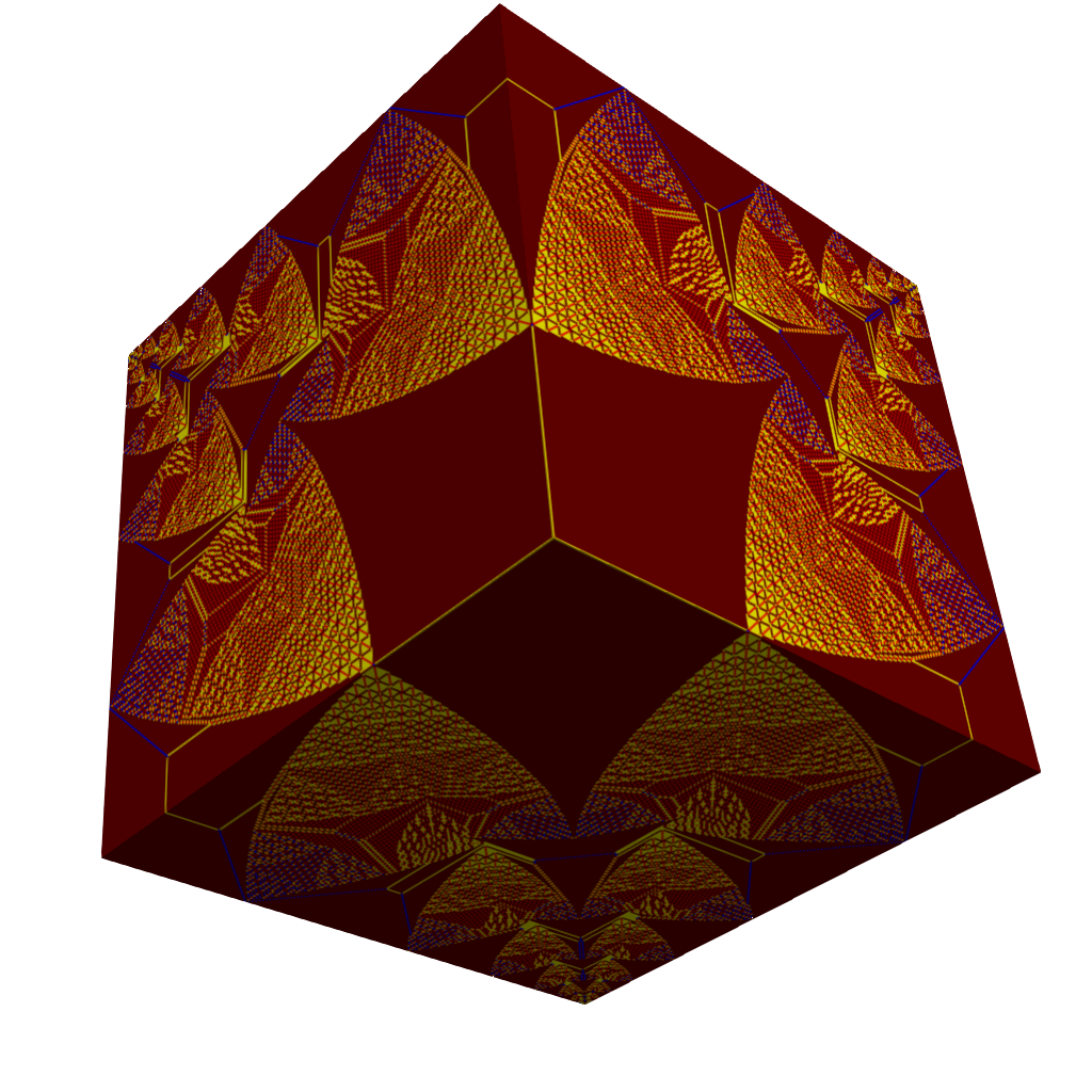
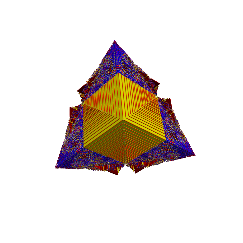
Figure 3. On the left, a corner cube of $s_{\infty}^{(N,3)}$ and on the right the same corner with all cross sections which match $s_{\infty}^{(N,2)}$ removed. The initial condition is $s_{0}\equiv 7$ and $N=2^{11}$. Sites with $0,\ldots,5$ chips are represented by different colors.

Problem 1.3.

Extend dimensional reduction on the hypercube to a domain of codimension zero.

The following is closely related.

Problem 1.4.

Show that the odometer for any bounded initial sandpile on the hypercube has bounded second differences. For instance, show for all $t\geq 1$ and $i=1,2$ that

$$-3\leq-2v_{t}(\mathbf{x})+v_{t}(\mathbf{x}+e_{i})+v_{t}(\mathbf{x}-e_{i})\leq 2$$

when $d=2$ and $s_{0}\equiv 4$.

Numerical evidence indicates the hypercube is a necessary hypothesis in Problem 1.4. In fact, in most other domains, including the discrete circle, the odometer does not appear to have bounded second differences. On the hypercube, our proof of dimensional reduction shows that the odometer has bounded second differences along the central cross sections; however, a method to propagate those bounds to the interior remains out of reach.

1.3. Outline of the proof

The proof of Theorem 1.1 is a careful induction on hypercube dimension, side length, and time. Some parts of the argument can be simplified but we present it in this fashion to suggest a template for proving dimensional reduction with more general initial data. At a high level, we show that if the parallel toppling process for a $d_{0}$-dimensional sandpile is sufficiently regular, then dimensional reduction is guaranteed in all dimensions $d>d_{0}$. We prove this regularity when $d_{0}=1$; the case $d_{0}>1$ remains open.

Our main technical tool is a technique introduced by Babai and Gorodezy to prove discrete quasiconcavity of the single-source sandpile odometer in $\mathbb{Z}^{2}$ [BG07]. By an iteration of their technique, we gain symmetry of the odometer, a derivative comparison result, and a parabolic least action principle. These results, which appear in Section 2, extend beyond the hypercube and so may be of independent interest.

In Section 3 we explicitly determine $v_{t}^{(d,N)}$ when $N=4$ in all dimensions $d\geq 1$ when the initial sandpile is $s_{0}\equiv 2d+d-1$. This is done by mapping the hypercube to a line via a radial decomposition. The explicit form of $v_{t}$ provides both a base case for our proof and progress towards Problem 1.2. We also show that when $N=2$ dimensional reduction does not occur at the critical dimension $d_{0}$.

The explicit solution when $N=4$ establishes the base case for an odometer regularity result which is then proved in Section 4. Finally, in Section 5, we use the established regularity of the odometer in dimension $(d-1)$ to prove dimensional reduction in dimension $d$

An efficient algorithm for computing high-dimensional sandpiles

In Section 2.4 we show that $v_{t}^{(d,N)}$ can be computed via the parallel toppling procedure restricted to the simplex. In fact, the argument shows that any sandpile with a symmetric initial condition on $\mathbb{Z}^{d}$, including the single-source sandpile, retains symmetry throughout the parallel toppling process and can be computed in this way.

For $d$ large, computing sandpiles on the simplex improves space complexity by a factor of $d^{d}$. Moreover, the reduction in size also leads to a faster algorithm when using parallelization. We wrote a program in Julia [BEKS17, BFDS18] for computing arbitrary dimensional sandpiles which implements these improvements. The program, which may be freely used and modified, is included in the arXiv post.

Acknowledgements

It is a pleasure to acknowledge Charles K. Smart for encouraging me to work on this problem and for many valuable conversations throughout. Additionally, I thank Lionel Levine for helpful discussions and for sharing past, unpublished, joint work with Alexander Holroyd and Karl Mahlburg towards the dimensional reduction conjecture. The anonymous referees provided detailed feedback which led to a much improved exposition.

2. Preliminaries

2.1. Notation and conventions

When we need to distinguish between vectors and scalars, we reserve $\mathbf{x}$ for vectors and $x$ for scalars. The $i$-th element of $\mathbf{x}$ is $x_{i}$ and $\mathbf{x}_{i}=(x_{1},\ldots,x_{i})$. We refer to coordinate basis vectors of $\mathbb{Z}^{d}$ as $e_{i}$ and the ones vector of length $i$ by $\mathbf{1}_{i}=(1,\ldots,1)$. Equalities, inequalities, addition, and multiplication between vectors and scalars are to be understood pointwise. The notation $|x|$ refers to the absolute value and $|\mathbf{x}|=\sum_{i=1}^{d}|x_{i}|$ is the $\ell_{1}$ norm.

We embed $\mathcal{C}_{N}^{(d)}$ into $\mathbb{Z}^{d}$ in two different ways depending on whether $N$ is even or odd. If $N=2k+1$, $\mathcal{C}_{N}^{(d)}=\{\mathbf{x}+1:|x_{i}|\leq k\}$ otherwise $\mathcal{C}_{N}^{(d)}=\{\mathbf{x}-k:1\leq x_{i}\leq 2k\}$. The graph Laplacian on $\mathcal{C}_{N}^{(d)}$ operates on functions $f:\mathcal{C}_{N}^{(d)}\to\mathbb{R}$ as

(3) $$\Delta^{(d)}f(x)=-2df(x)+\sum_{y\sim x}f(y),$$

where we pad $f(x):=0$ for $x\not\in\mathcal{C}_{N}^{(d)}$ and the sum $y\sim x$ is over the 2d nearest neighbors of $x$, $|y-x|=1$. When the hypercube size or dimension is not used, we omit distinguishing sub/superscripts.

2.2. Babai-Gorodezky technique

In this subsection and the next, let $s_{0}\leq 2(2d)-1$ be an arbitrary initial sandpile on $\mathcal{C}$ and $v_{t}$ its odometer. A straightforward induction argument and the definition of the graph Laplacian yields the following lemma.

Lemma 2.1.

For each $x\in\mathcal{C}$ and all $t\geq 0$,

(4) $$v_{t+1}(x)=\lfloor\frac{s_{0}(x)+\sum_{y\sim x}v_{t}(y)}{2d}\rfloor.$$

Babai and Gorodezky used this simple lemma to prove a nontrivial discrete quasiconcavity property of the single-source sandpile in $\mathbb{Z}^{d}$ [BG07]. A more general version of their argument appears below in Lemma 2.4. Roughly, their technique recognizes that if a property of the odometer holds at $t=1$, is consistent across the symmetry axes, and can be verified on the boundaries of the domain, it must hold for all $t\geq 1$.

Lemma 2.1 is used many other times throughout this paper; notably we use it to prove a parabolic least action principle and symmetry of the odometer on the hypercube.

2.3. Parabolic least action principle

The least action principle [FLP10] shows that $v_{\infty}$ is minimal among all $w:\mathcal{C}\to\mathbb{Z}^{+}$ which stabilize $s_{0}$: $\Delta w+s_{0}\leq 2d-1$. We upgrade this to a parabolic least action principle by observing the parallel toppling procedure as a directed sandpile on $\mathcal{G}=\mathbb{Z}^{+}\times\mathcal{C}$. The initial sandpile and odometer over time are stacked, $s(t,x):=s_{0}(x)$ and $v(t,x):=v_{t}(x)$ for all $t\geq 0$ and $x\in\mathcal{C}$. The graph Laplacian operates on functions $f:\mathcal{G}\to\mathbb{R}$ as

(5) $$\Delta^{\mathcal{G}}f(t,x)=-2df(t,x)+\sum_{y\sim x}f(t-1,y),$$

for $t\geq 1$ and $x\in\mathcal{C}$, where the sum $y\sim x$ is over the nearest neighbors of $x$ in $\mathcal{C}$.

Lemma 2.2 (Parabolic least action principle).

(6) $$v(t,x)=\min\{u:\mathcal{G}\to\mathbb{Z}^{+}:\Delta^{\mathcal{G}}u(t,x)+s(t,x)\leq 2d-1\mbox{ for all $x\in\mathcal{C}$ and $t\geq 1$}\}$$

Proof.

Let $w(t,x)$ denote the right-hand side of (6). We show using Lemma 2.1 and induction that $v(t,x)=w(t,x)$. Indeed, by the directed structure of $\mathcal{G}$, it suffices to show this equality one time slice at a time. Equality holds at $t=0$ as $v(0,x)=w(0,x)=0$. Assume that $v(t^{\prime},\cdot)=w(t^{\prime},\cdot)$ for $t^{\prime}\leq t$ and let $x\in\mathcal{C}$ be given. The monotonicity of the graph Laplacian implies $\Delta^{\mathcal{G}}w+s\leq 2d-1$, hence,

$$\Delta^{\mathcal{G}}w(t+1,x)+s(t+1,x)=-2dw(t+1,x)+s_{0}(x)+\sum_{y\sim x}w(t,y)<2d,$$

and a rearrangement yields,

$$w(t+1,x)\geq\lfloor\frac{s_{0}(x)+\sum_{y\sim x}w(t,y)}{2d}\rfloor.$$

By Lemma 2.1 and the inductive hypothesis, the right-hand side of the above is exactly $v(t+1,x)$. Similarly, for the other direction,

$$\Delta^{\mathcal{G}}v(t+1,x)+s(t+1,x) =2d\left(\frac{s_{0}(x)+\sum_{y\sim x}w(t,y)}{2d}-\lfloor\frac{s_{0}(x)+\sum_{y\sim x}w(t,y)}{2d}\rfloor\right)$$

$$<2d,$$

which concludes the proof by minimality of $w$. ∎

Our usage of the parabolic least action principle in the main argument is minimal and can be avoided. And, in some sense, it is a restatement of Lemma 2.1. We included it as it may be of independent interest.

2.4. Symmetry and fundamental domains

In this section we observe that sandpile dynamics on $\mathcal{C}_{N}^{(d)}$ preserve the symmetry structure of the $d$-dimensional hypercube. This is then used to reduce to the sandpile on a fundamental domain of the hypercube with reflecting boundary conditions. The main contribution of this subsection is a coordinate-wise description of this domain along with an explicit formula for the reflecting graph Laplacian.

We briefly provide a presentation of the group of automorphisms of the hypercube and its action on $\mathbb{Z}^{d}$; for more details see, for example, [GR13]. Let $\operatorname{Aut}_{\mathcal{C}_{d}}$ be the group of $(d\times d)$ matrices with exactly one $\pm 1$ in each row and in each column and $0$s elsewhere. Let $\sigma\in\operatorname{Aut}_{\mathcal{C}_{d}}$ act on $x\in\mathbb{Z}^{d}$ by matrix-vector multiplication followed by a translation and let it act on $f:\mathbb{Z}^{d}\to\mathbb{R}$ by $\sigma f(x):=f(\sigma x)$. The translation is chosen to preserve $\mathcal{C}_{N}^{(d)}$ when $N$ is even or odd in our choice of coordinates.

Each $\sigma$ is an isometry and hence preserves nearest neighbors and $\mathcal{C}^{(d)}_{N}$. That is, if $y\not\in\mathcal{C}^{(d)}_{N}$, then $\sigma y\not\in\mathcal{C}^{(d)}_{N}$. And, if $|y-x|=1$, then $|\sigma y-\sigma x|=1$, so

(7) $$\sum_{y^{\prime}\sim\sigma x}f(y^{\prime})=\sum_{y\sim x}f(\sigma y).$$

We say $\Omega\subseteq\mathcal{C}_{N}^{(d)}$ is a fundamental domain if there exists a set $\{\sigma_{1},\sigma_{2},\ldots\}\subset\operatorname{Aut}_{\mathcal{C}_{d}}$ so that $\bigcup_{j}\sigma_{j}\Omega=\mathcal{C}_{N}^{(d)}$. For example, a fundamental domain of an interval is half of it, while a fundamental domain of a square is a right triangle with one side along a central cross section of the square. The fundamental domains which we consider have coordinate consistency across dimensions. Let $M=\lceil N/2\rceil$ and

(8) $$\mathcal{S}^{(d)}_{M}:=\{(x_{1},\ldots,x_{d}):M\geq x_{1}\geq\cdots\geq x_{d}\geq 1\}.$$

Observe that $\{\mathbf{x}_{d-1}:(\mathbf{x}_{d-1},1)\in\mathcal{S}^{(d)}_{M}\}=\mathcal{S}^{(d-1)}_{M}$; this is the first step towards proving dimensional reduction on the hypercube.

Let $v_{t}$ be the odometer function for an initial sandpile, $s_{0}$, on $\mathcal{C}_{N}^{(d)}$ which is symmetric, $\sigma s_{0}=s_{0}$ for all $\sigma\in\operatorname{Aut}_{\mathcal{C}_{d}}$. We show that the parallel toppling odometer coincides with the symmetrized odometer $v_{t}^{\mathcal{S}}$ on $\mathcal{S}_{M}^{(d)}$ with appropriate reflecting boundary conditions. That is, for each $x\in\mathcal{S}_{M}^{(d)}$ and $y\sim x$ there exists a unique rotation or reflection, $\sigma_{y}\in\operatorname{Aut}_{\mathcal{C}_{d}}$, so that $\sigma_{y}y\in\mathcal{S}_{M}^{(d)}$. Let $y\overset{\mathcal{S}}{\sim}x$ denote iteration over the set $\{\sigma_{y}y:y\sim x\}$. For all $t\geq 0$ and $x\in\mathcal{S}_{M}^{(d)}$, let

(9) $$v_{t+1}^{\mathcal{S}}(x)=\lfloor\frac{s_{0}(x)+\sum_{y\overset{\mathcal{S}}{\sim}x}v_{t}^{\mathcal{S}}(y)}{2d}\rfloor,$$

where $v_{0}^{\mathcal{S}}:\equiv 0$.

We provide an algorithmic construction of this which we use to prove Lemma 2.4 below. Suppose $M\geq 2$, let $x\in\mathcal{S}_{M}^{(d)}$ be given and define $x_{0}=M$ and $x_{d+1}=1$. The following algorithm produces a sequence of indices describing the symmetrized nearest neighbors of $x$. Start with $l_{0}=0$ and pick the largest $(d+1)\geq r_{0}\geq l_{0}$ with $x_{l_{0}}=x_{r_{0}}$. If $r_{0}=(d+1)$, stop, otherwise, set $l_{1}=(r_{0}+1)$ and repeat, generating

(10) $$\mathbf{I}^{(M,d)}(x):=\{(l_{0},r_{0}),\ldots,(l_{n},r_{n})\},$$

where $n\leq(d+1)$. Observe that

$$M=x_{l_{0}}=x_{r_{0}}<\cdots<x_{l_{k}}=x_{r_{k}}<\cdots<x_{l_{n}}=x_{r_{n}}=1$$

so that

(11) $$\sum_{y\overset{\mathcal{S}}{\sim}x}v_{t}(y) =\sum_{k=1}^{n-1}(1+r_{k}-l_{k})\left(v_{t}(x-e_{r_{k}})+v_{t}(x+e_{l_{k}})\right)$$

$$+(r_{0}-l_{0})v_{t}(x-e_{r_{0}})$$

$$+(r_{n}-l_{n})(v_{t}(x-e_{r_{n}})+v_{t}(x+e_{l_{n}}))$$

where $v_{t}(x-e_{0})=v_{t}(x+e_{d+1}):=0$ and

(12) $$v_{t}(x-e_{r_{n}})=\begin{cases}v_{t}(x)&\mbox{ if $N$ is even }\\ v_{t}(x+e_{l_{n}})&\mbox{ if $N$ is odd}.\end{cases}$$

Lemma 2.3 (Symmetry).

For each $t\geq 0$ and each $\sigma\in\operatorname{Aut}_{\mathcal{C}_{d}}$, $\sigma v_{t}=v_{t}$. Hence, $v_{t}=v_{t}^{\mathcal{S}}$ on $\mathcal{S}^{(d)}_{M}$.

Proof.

We prove symmetry of $v_{t}$ by induction and Lemma 2.1. At $t=0$, $v_{t}\equiv 0$, so suppose symmetry holds at time $t$. Let $\sigma\in\operatorname{Aut}_{\mathcal{C}_{d}}$, $x\in\mathcal{C}_{N}^{(d)}$ be given. By Lemma 2.1, (7), and the inductive hypothesis,

$$v_{t+1}(\sigma x) =\lfloor\frac{s_{0}(\sigma x)+\sum_{y^{\prime}\sim\sigma x}v_{t}(y^{\prime})}{2d}\rfloor$$

$$=\lfloor\frac{s_{0}(\sigma x)+\sum_{y\sim x}v_{t}(\sigma y)}{2d}\rfloor$$

$$=\lfloor\frac{s_{0}(x)+\sum_{y\sim x}v_{t}(y)}{2d}\rfloor$$

$$=v_{t+1}(x).$$

∎

Note that the proof indicates that Lemma 2.3 can be extended in a natural way to other graphs and domains which are preserved under the automorphism group of the graph.

Henceforth, we consider $v_{t}^{\mathcal{S}}$ in $\mathcal{S}_{M}^{(d)}$ and drop all $\mathcal{S}$ superscripts. To reduce the number of cases with similar arguments, we only consider $N=2M$. Indeed, when $N$ is odd, the proofs are identical except for slight changes to the boundary arguments. Also, we will use $\mathcal{S}_{M}^{(d)}$ to refer exclusively to the sorted fundamental domain of $\mathcal{C}_{2M}^{(d)}$. The expressions $v_{t}^{(d,M)}$ and $s_{t}^{(d,M)}$ will refer to the parallel toppling odometers and sandpiles on $\mathcal{S}_{M}^{(d)}$.

2.5. Derivative comparison

In this section we provide a general parabolic comparison result for first order differences of $v_{t}$ on $\mathcal{S}_{M}$ when the initial sandpile, $s_{0}$, is constant. For $w\in\mathbb{Z}^{d}$, let $D_{w}$ denote a first order difference operator of the form $D_{w}v_{t}(\cdot)=v_{t}(\cdot)-v_{t}(\cdot+w)$. Pad $v_{t}$ by $v_{t}(x):=0$ for all $x\not\in\mathcal{C}_{N}$. Denote the interior with respect to $w$ as

(13) $$\mbox{Int}_{w}(\mathcal{S}_{M})=\{x\in\mathcal{S}_{M}:y^{\prime}\in\mathcal{S}_{M}\mbox{ for all $|y^{\prime}-(x+w)|=1$}\}$$

and the boundary as

(14) $$\partial_{w}\mathcal{S}_{M}=\mathcal{S}_{M}\backslash\mbox{Int}_{w}(\mathcal{S}_{M}).$$

Observe that every symmetrized $y\sim x\in\mathcal{S}_{M}$ is of the form $y=(x\pm e_{i})\mp d_{i}$, where $d_{i}$ is either a reflection, $d_{i}=e_{i}$ or a rotation $d_{i}=e_{i}-e_{j}$. We will show that if one can control $D_{w}v_{t}$ over the reflecting, rotating, and dissipating boundaries of $\mathcal{S}_{M}$, then that control persists over time. The dissipating boundary on $\mathcal{S}_{M}$ is

(15) $$\mathcal{B}^{(disp)}_{w}\mathcal{S}_{M}=\{x\in\mathcal{S}_{M}:(x+w)_{i}\geq M\mbox{ for some $1\leq i\leq d$}\}$$

while the reflecting and rotating boundaries are

(16) $$\mathcal{B}^{(ref)}_{w}\mathcal{S}_{M}=\{x\in\mathcal{S}_{M}:(x+w)_{i}\leq 1\mbox{ for some $1\leq i\leq d$}\}$$

and

(17) $$\mathcal{B}^{(rot)}_{w}\mathcal{S}_{M}=\{x\in\mathcal{S}_{M}:(x+w)_{i}\leq(x+w)_{j}\mbox{ for some $1\leq i<j\leq d$}\}.$$

For notational convenience write

(18) $$\mathcal{B}_{w}=\{\mathcal{B}^{(disp)}_{w}\cup\mathcal{B}^{(ref)}_{w}\cup\mathcal{B}^{(rot)}_{w}\}$$

and $\mathcal{B}_{w_{1},\ldots,w_{n}}=\cup_{i=1}^{n}\mathcal{B}_{w_{i}}$ for points $w_{i}\in\mathbb{Z}^{d}$. Note that in next lemma, we employ our convention to sometimes omit distinguishing sub/superscripts.

Lemma 2.4.

Let $\mathbf{w}:=\{w_{1},\ldots,w_{n}\}$ be a set of points in $\mathbb{Z}^{d}$ each equipped with a function $g_{j}:\mathcal{S}\to\mathbb{Z}$ which is superharmonic in the interior of $\mathcal{S}$. If

(19) $$\sup_{j}\left(D_{w_{j}}v_{t_{0}}(x)-g_{j}(x)\right)\leq 0\mbox{\qquad for all $x\in\mathcal{S}$}$$

and for all $t\geq t_{0}$ and $x\in\{\mathcal{B}_{0}\cup\mathcal{B}_{\mathbf{w}}\}\mathcal{S}$,

(20) $$\sup_{j} (\sum_{y\sim x}v_{t}(y)-\sum_{y^{\prime}\sim(x+w_{j})}v_{t}(y^{\prime})-2dg_{j}(x))\leq 0$$

  or

$$\sup_{j} (D_{w_{j}}v_{t+1}(x)-g_{j}(x))\leq 0$$

then

(21) $$\sup_{j}\left(D_{w_{j}}v_{t+1}(x)-g_{j}(x)\right)\leq 0$$

for all $t\geq t_{0}$ and $x\in\mathcal{S}$.

Proof.

We prove this by induction on $t$, starting at $t_{0}$, the base case guaranteed by (19). Suppose $\eqref{eq:derivative_comparison}$ holds at $t$ and let $w_{j}$, $x\in\mathcal{S}$ be given. First suppose $x\in\{\mbox{Int}_{w_{j}}\cap\mbox{Int}_{0}\}(\mathcal{S})$. By Lemma 2.1

$$D_{w_{j}}v_{t+1}(x)-g_{j}(x) \leq\lfloor\frac{(2d-1)+\sum_{y\sim x}v_{t}(y)-\sum_{y^{\prime}\sim(x+w_{j})}v_{t}(y^{\prime})}{2d}\rfloor-g_{j}(x)$$

$$=\lfloor\frac{(2d-1)+\sum_{y\sim x}D_{w_{j}}v_{t}(y)}{2d}\rfloor-g_{j}(x)$$

$$=\lfloor\frac{(2d-1)+\sum_{y\sim x}\left(D_{w_{j}}v_{t}(y)-g_{j}(y)\right)+\sum_{y\sim x}(g_{j}(y)-g_{j}(x))}{2d}\rfloor$$

$$\leq 0$$

as $g_{j}$ is superharmonic and integer-valued. If $x\in\{\mathcal{B}_{0}\cup\mathcal{B}_{w}\}$, then we either use the same argument or conclude depending on the case in (20).

∎

As a corollary, we deduce the following discrete quasiconcavity property of $v_{t}$ on a hypercube, which was proved in [BG07] for axis monotonic initial sandpiles on $\mathbb{Z}^{2}$. (Note that Aleksanyan and Shahgholian, using a discrete analogue of the method of moving planes, proved axis monotonicity of $v_{\infty}$ in [AS19].)

Corollary 2.1 (Axis monotonicity [BG07]).

For all $t\geq 1$, $x\in\mathcal{S}$, and all sets of indices

$$\mathcal{I}=\{i_{1},\ldots,i_{n}:1\leq i_{1}<\cdots<i_{n}\leq d\}$$

and

$$\mathcal{J}=\{j_{1},\ldots,j_{m}:i_{n}<j_{1}<\cdots<j_{m}\leq d\}$$

where $n\geq 1$ and $m\geq 0$ we have

$$v_{t}(x)\geq v_{t}(x+e_{\mathcal{I}}-e_{\mathcal{J}})\quad\mbox{for $(x+e_{\mathcal{I}}-e_{\mathcal{J}})\in\mathcal{S}$}$$

where $e_{\mathcal{I}}=\sum_{i\in\mathcal{I}}e_{i}$ denotes a sum over standard basis vectors indexed by $\mathcal{I}$.

We also have control on the derivative given an odometer upper bound on the dissipating boundary.

Corollary 2.2 (Derivative bound).

Suppose $v_{\infty}(M,\mathbf{1}_{d-1})\leq kM$ for integer $k\geq 1$. Then, for all $1\leq j\leq d$ and $t\geq 0$

(22) $$v_{t}(x)-v_{t}(x+e_{j})\leq kx_{j}.$$

Proof.

The claim is immediate if $M=1$, so suppose $M\geq 2$. Let $e_{j}$ and $x$ be given and let

(23) $$\mathbf{I}^{(M,d)}(x):=\{(l_{0},r_{0}),\ldots,(l_{n},r_{n})\},$$

be the indices describing the nearest neighbors of $x$ as defined in Section 2.4 above.

Pick the largest index $J$ so that

$$l_{J}\leq j\leq r_{J},$$

$v_{t}(x+e_{j})=v_{t}(x+e_{l_{J}})$, and (recalling $l_{J}=r_{J-1}+1$)

(24) $$\mathbf{I}^{(M,d)}(x+e_{l_{J}})=\begin{cases}\{\ldots,(l_{J-1},r_{J-1}+1),(l_{J}+1,r_{J}),\ldots\}&\mbox{ if $x_{r_{J-1}}=x_{l_{J}}+1$}\\ \{\ldots,(l_{J-1},r_{J-1}),(l_{J},l_{J}),(l_{J}+1,r_{J}),\ldots\}&\mbox{ if $x_{r_{J-1}}>x_{l_{J}}+1$}.\end{cases}$$

As $g_{j}(x):=kx_{j}$ is harmonic in the interior of $\mathcal{S}$, it remains to check (20) in Lemma 2.4. For later reference, we label the expression we bound,

(25) $$\sum_{y\sim x}v_{t}(y)-\sum_{y^{\prime}\sim(x+e_{l_{J}})}v_{t}(y^{\prime}).$$

The computations are similar in other cases, so we assume $x_{r_{J-1}}=x_{l_{J}}+1$ and $l_{J}+1\leq r_{J}$.

Case 1: $J=0$
As we are on the dissipating boundary, $v_{t+1}(x+e_{l_{J}})=0$ and $x_{l_{J}}=\cdots=x_{j}=M$, hence

$$v_{t+1}(x)-v_{t+1}(x+e_{l_{J}})=v_{t+1}(x)\leq v_{\infty}(M,\mathbf{1}_{d-1})\leq kM$$

by axis monotonicity and our assumption on the odometer.

Case 2: $1<J<n$
We compute (25), observing that all differences except for those near $r_{J}$ are unaffected by the symmetrization;

$$\eqref{eq:neighbor_sum} =\sum_{k=1,k\not\in[J-1,J]}^{n-1}(1+r_{k}-l_{k})(v_{t}(x-e_{r_{k}})-v_{t}(x-e_{r_{k}}+e_{l_{J}}))$$

$$+\sum_{k=1,k\not\in[J-1,J]}^{n-1}(1+r_{k}-l_{k})(v_{t}(x+e_{l_{k}})-v_{t}(x+e_{l_{k}}+e_{l_{J}}))$$

$$+(r_{0}-l_{0})(v_{t}(x-e_{r_{0}})-v_{t}(x-e_{r_{0}}+e_{l_{J}}))$$

$$+(r_{n}-l_{n})(v_{t}(x)-v_{t}(x+e_{l_{J}})+v_{t}(x+e_{l_{n}})-v_{t}(x+e_{l_{n}}+e_{l_{J}}))$$

$$+\star_{\{J-1,J\}}$$

$$\leq(2d-2(1+r_{J}-l_{J-1}))kx_{j}+\star_{\{J-1,J\}}$$

where $\star_{\{J-1,J\}}$ is defined as the sum of terms in the difference with indices $\{J-1,J\}$. This can then be computed,

$$\star_{\{J-1,J\}} =(1+r_{J}-l_{J})(v_{t}(x-e_{r_{J}})+v_{t}(x+e_{l_{J}}))$$

$$-(r_{J}-l_{J})(v_{t}(x+e_{l_{J}}-e_{r_{J}})+v_{t}(x+e_{l_{J}}+e_{l_{J}+1}))$$

$$+(1+r_{J-1}-l_{J-1})(v_{t}(x-e_{r_{J-1}})+v_{t}(x+e_{l_{J-1}}))$$

$$-(2+r_{J-1}-l_{J-1})(v_{t}(x+e_{l_{J}}-e_{l_{J}})+v_{t}(x+e_{l_{J}}+e_{l_{J-1}}))$$

$$\leq(r_{J}-l_{J})2kx_{j}+(1+r_{J-1}-l_{J-1})(k(x_{j}+1-1)+kx_{j})$$

$$+k(x_{j}-1)+k(x_{j}+1)$$

$$=2(1+r_{J}-l_{J-1})kx_{j}.$$

Case 3: $J=1<n$
We bound differences with indices $\{0,1\}$ in (25),

$$\star_{\{0,1\}} \leq(r_{0}-l_{0})kx_{l_{1}}$$

$$+(r_{1}-l_{1})2kx_{l_{1}}$$

$$+(v_{t}(x-e_{r_{1}})-v_{t}(x))+(v_{t}(x+e_{l_{1}})-0)$$

$$\leq(r_{0}-l_{0})kx_{l_{1}}+(r_{1}-l_{1})2kx_{l_{1}}+k(x_{l_{1}}-1)+k(x_{l_{1}}+1)$$

$$\leq 2(r_{1}-l_{0})kx_{l_{1}}.$$

Case 4: $J=n>1$
We bound differences with indices $\{n-1,n\}$ in (25),

$$\star_{\{n-1,n\}} \leq(1+r_{n-1}-l_{n-1})(k(x_{r_{n-1}}-1)+kx_{l_{n}})$$

$$+(r_{n}-l_{n}-1)(kx_{l_{n}}+kx_{l_{n}+1})$$

$$+(v_{t}(x)-v_{t}(x))+(v_{t}(x+e_{l_{n}})-v_{t}(x+e_{l_{n}}+e_{l_{n-1}}))$$

$$\leq(1+r_{n-1}-l_{n-1})2kx_{l_{n}}+(r_{n}-l_{n}-1)2kx_{l_{n}}$$

$$+k(x_{l_{n-1}})$$

$$\leq 2(r_{n}-l_{n-1})kx_{l_{n}}.$$

In the last step we used $x_{l_{n-1}}=x_{l_{n}}+1=2x_{l_{n}}$.

Case 5: $J=n=1$
We bound differences with indices $\{0,n\}$ in (25),

$$\star_{\{0,n\}} \leq(r_{0}-l_{0})(k(x_{r_{0}}-1))$$

$$+(r_{n}-l_{n}-1)(kx_{l_{n}}+kx_{l_{n}+1})$$

$$+(v_{t}(x+e_{l_{n}})-0)+(v_{t}(x)-v_{t}(x))$$

$$\leq(r_{0}-l_{0})2kx_{l_{n}}+(r_{n}-l_{n}-1)2kx_{l_{n}}$$

$$+kx_{l_{n}}$$

$$\leq 2(r_{n}-l_{0}-1)kx_{l_{n}}.$$

∎

2.6. Weak topple control

We provide a difference-in-time analogue of Lemma 2.4

Lemma 2.5.

For all $t\geq t_{0}$ and $j\geq 0$,

$$\max_{z\in\mathcal{S}}\left(v_{t+j}(z)-v_{t}(z)\right)\leq\max_{z\in\mathcal{S}}\left(v_{t_{0}+j}(z)-v_{t_{0}}(z)\right)$$

Proof.

We induct on $t$ starting at $t_{0}$. Suppose the result holds for $(t-1)$ and let $x\in\mathcal{S}$ be given. Lemma 2.1 implies

$$v_{t+j}(x)-v_{t}(x)\leq\lfloor\frac{(2d-1)+\sum_{y\sim x}\left(v_{t+j-1}(y)-v_{t-1}(y)\right)}{2d}\rfloor,$$

hence, by induction

$$v_{t+j}(x)-v_{t}(x)\leq\lfloor\frac{(2d-1)+2d\left(\max_{z\in\mathcal{S}}\left(v_{t_{0}+j}(z)-v_{t_{0}}(z)\right)\right)}{2d}\rfloor=\max_{z\in\mathcal{S}}\left(v_{t_{0}+j}(z)-v_{t_{0}}(z)\right).$$

∎

3. Explicit solutions when $M\leq 2$

In this section, we compute $v_{t}^{(d)}$ when $s_{0}^{(d)}\equiv 2d+(d-1)$ for all $d\geq 1$ when $M=2$. We also show that dimensional reduction does not occur at dimension $d=d_{0}$ when $s^{(d)}_{0}\equiv 2d+(d_{0}-1)$ and $M=1$.

3.1. $M=1$

As we do not know how to define a $0$-dimensional sandpile, suppose $d_{0}\geq 2$.

Proposition 3.1.

When $s_{0}^{(d)}\equiv 2d+(d_{0}-1)$, $v_{\infty}^{(d_{0})}\equiv 1$ but $v_{\infty}^{(d_{0}-1)}\equiv 2$.

Proof.

In dimension $d$, a corner site of the hypercube has $d$ internal neighbors so $\Delta^{(d)}(\mathbf{1})=-2d+d=-d$. Hence, in dimension $d_{0}$,

$$s_{1}^{(d_{0})}(\mathbf{1})=(2d_{0}+(d_{0}-1))-d_{0}=2d_{0}-1$$

however, in dimension $(d_{0}-1)$,

$$s_{1}^{(d_{0}-1)}(\mathbf{1})=(2(d_{0}-1)+(d_{0}-1))-(d_{0}-1)=2(d_{0}-1).$$

∎

3.2. $M=2$

Now, suppose $d\geq 1$. After a radial reparameterization of $\mathcal{S}_{2}$, arbitrary dimensional sandpiles become one-dimensional with a simple nearest-neighbor toppling rule. Indeed, every $\mathbf{x}\in\mathcal{S}_{2}$ is of the form $\mathbf{x}=(\mathbf{2}_{x},\mathbf{1}_{d-x})$, for $x=0,\ldots,d$. Overload notation and consider $s_{t}$ and $v_{t}$ as functions on $\{0,\ldots,d\}$. The Laplacian on the one-dimensional graph can then be computed using symmetry.

Lemma 3.1.

If we define $0=v_{t}(d+1)=v_{t}(-1)$, then

$$\Delta v_{t}(x)=(-d-x)v_{t}(x)+(d-x)v_{t}(x+1)+xv_{t}(x-1).$$

Proof.

Let $\mathbf{x}=(\mathbf{2}_{x},\mathbf{1}_{d-x})$ so that $\mathbf{I}^{(2,d)}(\mathbf{x})=\{(0,x),(x+1,d+1)\}$. Hence, by definition of the symmetric Laplacian,

$$\Delta v_{t}(\mathbf{x}) =-2dv_{t}(\mathbf{x})+xv_{t}(\mathbf{x}-e_{x})+(d-x)(v_{t}(\mathbf{x})+v_{t}(\mathbf{x}+e_{x+1}))$$

$$=-2dv_{t}(x)+(d-x)v_{t}(x)+(d-x)v_{t}(x+1)+xv_{t}(x-1).$$

∎

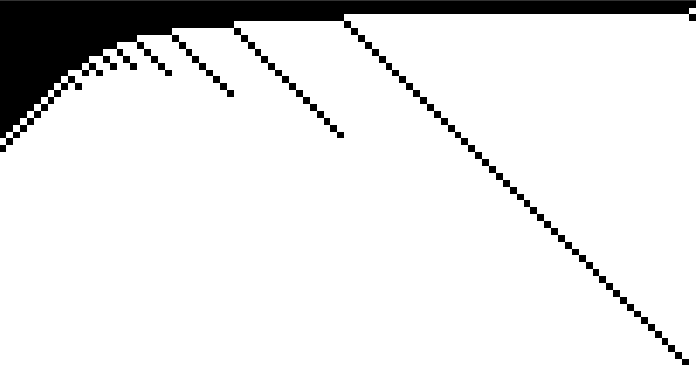
Figure 4. The parallel toppling odometer for $s_{0}\equiv 2d+(d-1)$ when $d=100$ and $M=2$. A black pixel in row $t$ and column $x$ indicates that $v_{t}(x)=v_{t-1}(x)+1$. The top row is $t=0$ and $t$ increases from top to bottom. The left column is $x=1$ and $x$ increases from left to right.

See Figure 4 for a display of the odometer throughout the parallel toppling process when $s^{(d)}_{0}\equiv 2d+(d-1)$ in dimension $d=100$. Visually, a contiguous block of decreasing size fires at each step, followed by a ripple of outwards firings. For $t>t_{d}:=(\lceil\sqrt{d-1}\rceil+1)$, the firing block appears to decreases by one every step. In particular, if $a_{t}$ indexes the right edge of the block at time $t$, then $a_{1}=d$ and

$$a_{t}=\begin{cases}\lfloor\frac{d-1}{t-1}\rfloor&\mbox{ for $t\leq t_{d}$ }\\ a_{t-1}-1&\mbox{ for $t>t_{d}$}.\end{cases}$$

This leads to a simple formula for $v_{t}$.

Proposition 3.2.

For all $d\geq 1$, when $s_{0}^{(d)}=2d+(d-1)$, the radially reparameterized parallel toppling odometer has the following form. For all $t\geq 1$,

(26) $$v_{t}(x)=\begin{cases}v_{t-1}(x)+1&\mbox{ for $x\leq a_{t}$}\\ v_{t-1}(x)&\mbox{ for $a_{t}<x\leq a_{t-1}$}.\end{cases}$$

And for each $t^{\prime}<t$ and $a_{t^{\prime}-1}\geq x>a_{t^{\prime}}$

(27) $$v_{t}(x)=v_{t-1}(x-1).$$

Proof.

We induct on $t$. Since $s_{0}\geq 2d$, $v_{1}\equiv 1$. Suppose (26) and (27) hold for all $t^{\prime}\leq t$.

Step 1: (26)
By strong induction for $t^{\prime}\leq t$, (26) implies $v_{t}(x)=t$ for $x\leq a_{t}$. Thus,

$$s_{t}(x)=\begin{cases}2d+(d-1)-tx&\mbox{ for $x<a_{t}$}\\ 2d+(d-1)-tx-(d-x)&\mbox{ for $x=a_{t}$}.\end{cases}$$

Let $g(x):=(d-1)-tx$. If $g(x)\geq 0$, $v_{t+1}(x)=v_{t}(x)+1$, otherwise $v_{t+1}(x)=v_{t}(x)$. When $a_{t+1}<x\leq a_{t}$, $g(x)<0$. Indeed, $g(a_{t+1})\leq(t-1)$ and $g(x+1)-g(x)=-t$.

As $g$ is increasing in $x$, it remains to check $g(a_{t+1})\geq 0$ for all $t$. If $x\leq\frac{d-1}{t}$ then $g(x)\geq 0$. If $(t+1)>t_{d}$, then

$$\frac{d-1}{t-1}-\frac{d-1}{t}\leq\frac{d-1}{\sqrt{d-1}\left(\sqrt{d-1}+1\right)}\leq 1,$$

thus

$$a_{t+1} =a_{t}-1$$

$$\leq\frac{d-1}{t-1}-1$$

$$\leq\frac{d-1}{t}.$$

Step 2: (27)

Now, take $a_{t^{\prime}-1}\geq x>a_{t^{\prime}}$ for $1\leq t^{\prime}\leq(t-1)$. If $v_{t}(x-1)=v_{t}(x)+1$, then by strong induction for $t^{\prime}\leq t$, (27) and (26) imply that $v_{t}(x-2)=v_{t}(x-1)=t^{\prime}$ and $v_{t}(x)=t^{\prime}-1=v_{t}(x+1)$. Thus,

$$s_{t}(x) \geq 2d+(d-1)-(t^{\prime}-2)x$$

$$\geq 2d+(d-1)-(t^{\prime}-2)a_{t^{\prime}-1}$$

$$\geq 2d+(d-1)-(d-1)$$

$$=2d.$$

However,

$$s_{t}(x-1) =2d+(d-1)-t^{\prime}x-d+x$$

$$=2d-1-(t^{\prime}-1)x$$

$$\leq 2d-1,$$

as $t^{\prime}\geq 1$. If $v_{t}(x-1)=v_{t}(x)=v_{t}(x+1)=(t^{\prime}-1)$, then

$$s_{t}(x) \leq 2d+(d-1)-(t^{\prime}-1)x$$

$$<2d+(d-1)-(t^{\prime}-1)(a_{t^{\prime}})$$

$$\leq 2d.$$

∎

4. Odometer regularity when $d=1$

From here onward, suppose $s_{0}\equiv 2d$. We start the inductive proof of Theorem 1.1 by establishing some regularity of the odometer in the critical dimension $d=d_{0}=1$. In the next section, we inductively use dimensional reduction to show that $d\geq 2$ sandpiles inherit this regularity. This regularity ensures that the dynamics of lower-dimensional sandpiles agree with their higher-dimensional embeddings.

When reading Section 5 below, the reader should observe that whenever Proposition 4.1 (or something close to it) holds, dimensional reduction follows. For example, if a version of this result is established in every critical dimension $d_{0}\geq 1$, then dimensional reduction follows for all sandpiles of the form $2d+(d_{0}-1)$ in dimensions $d>d_{0}$. Proposition 3.2 should be understood as a step in this direction.

Proposition 4.1.

Recall the definition of $\tau_{j}$ from Theorem 1.1. For all $M\geq 2$ and $d\geq 1$, the odometer maintains the following properties throughout the parallel toppling process.

Self-similarity:

For each $1\leq j\leq M$ and $t\leq\tau_{j}$

(28) $$v_{t}^{(M)}(\mathbf{x})=v_{t}^{(j)}(\mathbf{x}-(M-j))\mbox{ for $\mathbf{x}>M-j$}.$$

Weak facet compatibility:

For all $\mathbf{x}_{i}\geq 2$, $t\geq 1$, $i\geq 0$, $j\geq 0$ and $i+j+1=d$

(29) $$v_{t}^{(M)}(\mathbf{x}_{i},1,\mathbf{1}_{j}) =v_{t}^{(M)}(\mathbf{x}_{i},2,\mathbf{1}_{j})+1$$

$$\implies$$

$$v_{t+1}^{(M)}(\mathbf{x}_{i},1,\mathbf{1}_{j}) =v_{t+1}^{(M)}(\mathbf{x}_{i},1,\mathbf{1}_{j}).$$

Strong facet compatibility:

For all $\mathbf{x}_{i}\geq 2$, $j\geq 0$, $i<d$, ($t<\tau_{M}$ and $i\geq 0$) or ($i\geq 1$ and $t\geq\tau_{M}$)

(30) $$v_{t}^{(M)}(\mathbf{x})-v_{t}^{(M)}(\mathbf{x}+2e_{i+1})\leq 2$$

and

(31) $$v_{t}^{(M)}(\mathbf{x}_{i},1,\mathbf{1}_{j}) =v_{t}^{(M)}(\mathbf{x}_{i},2,\mathbf{1})+1$$

$$\implies$$

$$v_{t+1}^{(M)}(\mathbf{x}_{i},1,\mathbf{1}_{j}) =v_{t}^{(M)}(\mathbf{x}_{i},1,\mathbf{1}_{j})$$

$$v_{t+1}^{(M)}(\mathbf{x}_{i},2,\mathbf{1}_{j}) =v_{t}^{(M)}(\mathbf{x}_{i},2,\mathbf{1}_{j})+1.$$

Strong topple control:

For all $t\geq\tau_{M-1}$,

(32) $$\sup_{\mathbf{x}\in\mathcal{S}_{M}}\left(v_{t+2}(\mathbf{x})-v_{t}(\mathbf{x})\right)\leq 1.$$

Proof of Proposition 4.1 for $d=d_{0}=1$.

The proof proceeds by induction on $M$ and then on $t$. When $M=2$,

	$v_{t}^{(M)}(1)$	$v_{t}^{(M)}(2)$
$t=1$	1	1
$t=2$	2	1
$t=3$	2	2
$t=4$	3	2

and $v_{1}^{(M-1)}(1)=v_{2}^{(M-1)}(1)=1$ which verifies the base case. Now, let $M$ be given and note that $v_{1}^{(M)}(x)=1$ for all $1\leq x\leq M$ and $v_{2}^{(M)}(x)=2$ for $1\leq x<M$ and $v_{2}^{(M)}(M)=1$. Hence, suppose (28),(29),(30),(31), hold for $(M-1)$ for all $t\geq 1$ and suppose they hold for $M$ for all $t^{\prime}\leq(t-1)$. We verify each inductive step.

Self-similarity: (28)

By strong induction, it suffices to show $v_{t}^{(M)}(x)=v_{t}^{(M-1)}(x-1)$ for $x\geq 2$. By Lemma 2.1,

$$v_{t}^{(M)}(x)=1+\lfloor\frac{v_{t-1}^{(M)}(x+1)+v_{t-1}^{(M)}(x-1)}{2}\rfloor$$

for $x>1$. Hence, by (28) at $(t-1)$, for $x>2$,

$$v_{t}^{(M)}(x)=1+\lfloor\frac{v_{t-1}^{(M-1)}(x)+v_{t-1}^{(M-1)}(x-2)}{2}\rfloor=v_{t}^{(M-1)}(x-1).$$

For $x=1$, we have reflection at the origin,

$$v_{t}^{(M-1)}(1)=1+\lfloor\frac{v_{t-1}^{(M-1)}(2)+v_{t-1}^{(M-1)}(1)}{2}\rfloor=1+\lfloor\frac{v_{t-1}^{(M)}(3)+v_{t-1}^{(M)}(2)}{2}\rfloor.$$

Hence, if $v_{t-1}^{(M)}(1)=v_{t-1}^{(M)}(2)$, then $v_{t}^{(M-1)}(1)=v_{t}^{(M)}(2)$.

When $v_{t-1}^{(M)}(1)=v_{t-1}^{(M)}(2)+1$, we instead use strong facet compatibility in both layers. If $v_{t-1}^{(M-1)}(1)=v_{t-1}^{(M-1)}(2)$, then $v_{t}^{(M-1)}(1)=v_{t-1}^{(M-1)}(1)+1$ and we are done, so suppose not. Since sites topple at most once per time step by Lemma 2.5, the odometer must then be, for some $v\geq 2$:

	$v_{\cdot}^{(M)}(1)$	$v_{\cdot}^{(M)}(2)$	$v_{\cdot}^{(M)}(3)$
$t-2$	$v$	$v$	$v-1$
$t-1$	$v+1$	$v$	$v-1$
$t$	$v+1$	$v+1$	$\geq(v-1)$

This contradicts strong facet compatibility for $v_{t}^{(M-1)}(1)$ from $(t-2)\to(t-1)$, which we can use as $t\leq\tau_{M-1}$ and hence $(t-1)<\tau_{M-1}$.

Weak facet compatibility: (29)

If $v_{t}(1)=v_{t}(2)+1$, then $\Delta v_{t}(1)=-1$ and so $v_{t+1}(1)=v_{t}(1)$.

Strong facet compatibility: (30) and (31)

We use Lemma 2.4 to show (30). The function $g(x)=2x$ is harmonic in the interior of the interval so it suffices to check the dissipating and reflecting boundaries. We control the dissipating boundary using $t<\tau_{M}$ and the reflecting boundary with (29).

As $t<\tau_{M}$, $v_{t}(M)\leq(M-1)$ and hence by Corollary 2.2, $v_{t}(M-1)\leq v_{t}(M)+(M-1)\leq 2(M-1)$. For the reflecting boundary, i.e, $x=1$, we check

$$\sum_{y\sim x}v_{t}(y)-\sum_{y^{\prime}\sim(x+2)}v_{t}(y) =(v_{t}(1)-v_{t}(2))+(v_{t}(2)-v_{t}(4))\leq(v_{t}(1)-v_{t}(2))+4.$$

If $v_{t}(1)-v_{t}(2)=1$, then $v_{t+1}(1)=v_{t}(1)$ by weak facet compatibility. Otherwise, $\sum_{y\sim x}v_{t}(y)-\sum_{y^{\prime}\sim(x+2)}v_{t}(y)\leq 4$ and we conclude that

$$v_{t}(x)-v_{t}(x+2)\leq 2x.$$

Taking $x=1$, this implies

$$\Delta v_{t}(2)\geq-2v_{t}(2)+v_{t}(1)+v_{t}(1)-2\geq 0,$$

which shows (31).

Strong topple control: (32)

By Lemma 2.5, it suffices to show

$$\sup_{x\in\mathcal{S}_{M}}\left(v_{\tau_{M-1}+2}(x)-v_{\tau_{M-1}}(x)\right)\leq 1$$

First observe that (28) for $v_{t}^{(M)}$ and (32) for $v_{t}^{(M-1)}$ imply that

(33) $$\tau_{M-1}\geq\tau_{M-2}+2.$$

Suppose for sake of contradiction that

$$\left(v_{\tau_{M-1}+2}(x)-v_{\tau_{M-1}}(x)\right)=2$$

for some $1\leq x\leq M$. Lemma 2.5 then implies that some neighbor $y\sim x$ must have toppled twice previously. Pick the maximal such $y$. We consider three cases for $y$.

Case 1: $y\geq 3$
We first note that $v_{\tau_{M-1}+1}^{(M)}(y)=v_{\tau_{M-1}+1}^{(M-1)}(y-1)$. Indeed, by (28), as $(y-1)\geq 2$,

$$v_{\tau_{M-1}+1}^{(M)}(y) =1+\lfloor\frac{v_{\tau_{M-1}}^{(M)}(y+1)+v_{\tau_{M-1}}^{(M)}(y-1)}{2}\rfloor$$

$$=1+\lfloor\frac{v_{\tau_{M-1}}^{(M-1)}(y)+v_{\tau_{M-1}}^{(M-1)}(y-2)}{2}\rfloor$$

$$=v_{\tau_{M-1}+1}^{(M-1)}(y-1)$$

Hence,

$$2=v_{\tau_{M-1}+1}^{(M)}(y)-v_{\tau_{M-1}-1}^{(M)}(y)=v_{\tau_{M-1}+1}^{(M-1)}(y-1)-v_{\tau_{M-1}-1}^{(M-1)}(y-1),$$

which contradicts (32) for $v_{t}^{(M-1)}$.

Case 2: $y=2$
We claim that $v_{\tau_{M-1}+1}^{(M)}(2)=v_{\tau_{M-1}+1}^{(M-1)}(1)$, in which case we can use the argument of Case 1. If not, then $v_{\tau_{M-1}}^{(M)}(2)=v_{\tau_{M-1}}^{(M)}(3)+1$ but $v_{\tau_{M-1}}^{(M)}(1)=v_{\tau_{M-1}}^{(M)}(2)+1$. This implies that either

$$v_{\tau_{M-1}-1}^{(M)}(1)=v_{\tau_{M-1}-1}^{(M)}(2)+2$$

or

$$v_{\tau_{M-1}-1}^{(M)}(1) =v_{\tau_{M-1}-1}^{(M)}(2)+1$$

and

$$v_{\tau_{M-1}}^{(M)}(1) =v_{\tau_{M-1}-1}^{(M)}(1)+1$$

both which contradict weak facet compatibility.

Case 3: $y=1$
In this case, the odometer near the center must be, for some $v\geq 1$,

	$v_{\cdot}^{(M)}(1)$	$v_{\cdot}^{(M)}(2)$	$v_{\cdot}^{(M)}(3)$
$\tau_{M-1}-1$	$v$	$v$	$v$
$\tau_{M-1}$	$v+1$	$v+1$	$v$
$\tau_{M-1}+1$	$v+2$	$v+1$	$\geq(v)$

This shows $v^{(M)}_{\tau_{M-1}-2}(2)=v-1$. Indeed, if $v^{(M)}_{\tau_{M-1}-2}(1)=v-1$, then as $\Delta v^{(M)}_{\tau_{M-1}-2}(1)\geq 0$ $v^{(M)}_{\tau_{M-1}-2}(2)=v-1$. If $v^{(M)}_{\tau_{M-1}-2}(1)=v$, then $\Delta v^{(M)}_{\tau_{M-1}-2}(1)\leq-1$ and $v^{(M)}_{\tau_{M-1}-2}(2)=v-1$. Hence,

$$v^{(M-1)}_{\tau_{M-1}}(1)=v^{(M)}_{\tau_{M-1}}(2)=v^{(M)}_{\tau_{M-1}-2}(2)+2=v^{(M-1)}_{\tau_{M-1}-2}(2)+2,$$

which contradicts (32) for $v_{t}^{(M-1)}$ using (33).

∎

Note that the comparison principle for sandpiles (see, for example, Proposition 3.3 in [BR21]) shows

$$v_{\infty}(x)=\frac{1}{2}\left(M(M+1)-x(x-1)\right),$$

and so $v_{\infty}(x)-v_{\infty}(x+1)=x$. Hence we must use an assumption like $t<\tau_{M}$ for strong facet compatibility.

5. Odometer regularity and dimensional reduction

We now prove Proposition 4.1 for $d\geq 2$ together with dimensional reduction,

(34) $$v_{t}^{(d,M)}(\mathbf{x}_{d-1},1)=v_{t}^{(d-1,M)}(\mathbf{x}_{d-1}),$$

by strong induction on $M$, $d$, and $t$. Specifically, given $M$, $d$, and $t$, suppose

$$\eqref{base_dimension:consistency},\eqref{base_dimension:weak_compatability},\eqref{base_dimension:strong_derivative},\eqref{base_dimension:strong_compatability},\eqref{base_dimension:strong_topple}$$

hold for

$$v_{t^{\prime}}^{(d^{\prime},M^{\prime})} \quad\mbox{for all $M^{\prime}\geq 1$, $t^{\prime}\geq 1$, $d^{\prime}<d$},$$

$$v_{t^{\prime}}^{(d,M^{\prime})} \quad\mbox{for all $M^{\prime}<M$, $t^{\prime}\geq 1$},$$

$$v_{t^{\prime}}^{(d,M)} \quad\mbox{for all $t^{\prime}<t$}.$$

We also suppose (34) holds for $v_{t-1}^{(d^{\prime},M^{\prime})}$ for all $d^{\prime}\geq 2$ and $M^{\prime}\leq M$. Indeed, $v_{1}^{(d,M)}\equiv 1$ for all $d\geq 1$ and $M\geq 1$.

5.1. Dimensional reduction

We start the induction in time by proving dimensional reduction given odometer regularity at $(t-1)$. Let $\mathbf{x}_{d-1}$ be given and pick the smallest $d>i\geq 0$ so that $(\mathbf{x}_{i},\mathbf{1}_{d-i})=(\mathbf{x}_{d-1},1)$. By symmetry,

$$\Delta^{(d)}v_{t-1}^{(d)}(\mathbf{x}_{i},\mathbf{1}_{d-i}) =-2dv_{t-1}^{(d)}(\mathbf{x}_{i},\mathbf{1}_{d-i})$$

$$+\sum_{\mathbf{y}_{i}\sim\mathbf{x}_{i}}v_{t-1}^{(d)}(\mathbf{y}_{i},\mathbf{1}_{d-i})$$

$$+(d-i)\left(v_{t-1}^{(d)}(\mathbf{x}_{i},\mathbf{1}_{d-i})+v_{t-1}^{(d)}(\mathbf{x}_{i},2,\mathbf{1}_{d-i-1})\right).$$

We consider two cases at time $(t-1)$.

Case 1: $v_{t-1}^{(d)}(\mathbf{x}_{i},\mathbf{1}_{d-i})=v_{t-1}^{(d)}(\mathbf{x}_{i},2,\mathbf{1}_{d-i-1})$

By (34) at $(t-1)$, $v_{t-1}^{(d)}(\mathbf{x}_{i},\mathbf{1}_{d-i})=v_{t-1}^{(i+1)}(\mathbf{x}_{i},1)$. Thus,

$$\Delta^{(d)}v_{t-1}^{(d,M)}(\mathbf{x}_{i},\mathbf{1}_{d-i}) =-2iv_{t-1}^{(i+1)}(\mathbf{x}_{i},1)+\sum_{\mathbf{y}_{i}\sim\mathbf{x}_{i}}v_{t-1}^{(i+1)}(\mathbf{y}_{i},1)$$

$$=\Delta^{(i+1)}v_{t-1}^{(i+1,M)}(\mathbf{x}_{i},1)$$

which concludes this case as $v_{t}^{(d)}=v_{t-1}^{(d)}+1(\Delta^{(d)}v_{t-1}^{(d)}\geq 0)$.

Case 2: $v_{t-1}^{(d)}(\mathbf{x}_{i},\mathbf{1}_{d-i})=v_{t-1}^{(d)}(\mathbf{x}_{i},2,\mathbf{1}_{d-i-1})+1$
If $i\leq(d-2)$, then (29) for $(t-1)\to t$ for both $v_{t-1}^{(i+1)}$ and $v_{t-1}^{(d)}$ imply that

$$v_{t-1}^{(i+1)}(\mathbf{x}_{i},1)=v_{t-1}^{(d)}(\mathbf{x}_{i},\mathbf{1}_{d-i})=v_{t}^{(d)}(\mathbf{x}_{i},\mathbf{1}_{d-i})=v_{t}^{(i+1)}(\mathbf{x}_{i},1).$$

If $i=(d-1)$, then (31) and (34) at $(t-1)$ and $(t-2)$ imply that

$$v_{t-1}^{(d-1)}(\mathbf{x}_{d-1})=v_{t-1}^{(d)}(\mathbf{x}_{d-1},1)=v_{t-2}^{(d)}(\mathbf{x}_{d-1},1)+1=v_{t-2}^{(d-1)}(\mathbf{x}_{d-1})+1.$$

If $(t-2)\geq\tau_{M-1}$, (32) for $v_{t}^{(i)}$ and $v_{t}^{(d)}$ imply that

$$v_{t}^{(d-1)}(\mathbf{x}_{d-1})=v_{t-1}^{(d-1)}(\mathbf{x}_{d-1})=v_{t-1}^{(d)}(\mathbf{x}_{d-1},1)=v_{t}^{(d)}(\mathbf{x}_{d-1},1).$$

If $(t-2)<\tau_{M-1}$, then (28) and (34) for $v_{t-1}^{(M-1)}$ show

$$v_{t-1}^{(d,M)}(\mathbf{x}_{d-1},2)=v_{t-1}^{(d,M-1)}(\mathbf{x}_{d-1}-1,1)=v_{t-1}^{(d-1,M-1)}(\mathbf{x}_{d-1}-1).$$

Similarly,

$$v_{t-1}^{(d,M)}(\mathbf{x}_{d-1},1)=v_{t-1}^{(d-1,M)}(\mathbf{x}_{d-1})=v_{t-1}^{(d-1,M-1)}(\mathbf{x}_{d-1}-1).$$

Therefore, for all $t^{\prime}\leq\tau_{M-1}$,

(35) $$v_{t^{\prime}}^{(d,M)}(\mathbf{x}_{d-1},2)=v_{t^{\prime}}^{(d,M)}(\mathbf{x}_{d-1},1),$$

this however contradicts the case we are in.

5.2. Odometer regularity for $d\geq 2$

We verify each inductive step.

Self-similarity: (28)

As $\eqref{base_dimension:consistency}$ holds for $(M-1)$ at $t$, it suffices to show that if $t\leq\tau_{M-1}$ and $\mathbf{x}>1$,

(36) $$v_{t}^{(M)}(\mathbf{x})=v_{t}^{(M-1)}(\mathbf{x}-1).$$

We split verification of this into cases.

Case 1: $\mathbf{x}>2$
As (36) holds for $(t-1)$, by Lemma 2.1,

$$v_{t}^{(M)}(\mathbf{x}) =\lfloor\frac{s_{0}(\mathbf{x})+\sum_{\mathbf{y}\sim\mathbf{x}}v_{t-1}^{(M)}(\mathbf{y})}{2d}\rfloor$$

$$=\lfloor\frac{s_{0}(\mathbf{x}-1)+\sum_{\mathbf{y}\sim(\mathbf{x}-1)}v_{t-1}^{(M-1)}(\mathbf{y})}{2d}\rfloor$$

$$=v_{t}^{(M-1)}(\mathbf{x}-1).$$

Case 2: $\mathbf{x}=(\mathbf{x}_{j},\mathbf{2})$ for $\mathbf{x}_{j}>2$ and $0\leq j<d$
We show that if $\Delta v_{t-1}^{(M)}(\mathbf{x})\geq 0$, then $\Delta v_{t-1}^{(M-1)}(\mathbf{x}-1)\geq 0$. First, decompose the Laplacian into a sum of discrete second differences,

$$\Delta v_{t-1}^{(M)}(\mathbf{x})=\sum_{i=1}^{d}\Delta_{(i)}v_{t-1}^{(M)}(\mathbf{x}),$$

where

$$\Delta_{(i)}v_{t-1}^{(M)}(\mathbf{x})=-2v_{t-1}^{(M)}(\mathbf{x})+v_{t-1}^{(M)}(\mathbf{x}+e_{i})+v_{t-1}^{(M)}(\mathbf{x}-e_{i}).$$

Observe that (28) at $(t-1)$ implies, $\Delta_{(i)}v_{t-1}^{(M)}(\mathbf{x})=\Delta_{(i)}v_{t-1}^{(M-1)}(\mathbf{x}-1)$ for all $i\leq j$ and for $i>j$,

$$\Delta_{(i)}(v_{t-1}^{(M-1)}(\mathbf{x}-1)-v_{t-1}^{(M)}(\mathbf{x}))=v_{t-1}^{(M-1)}(\mathbf{x}-e_{i}-1)-v_{t-1}^{(M)}(\mathbf{x}-e_{i}).$$

By reflectional symmetry, for each $i>j$,

$$v_{t-1}^{(M-1)}(\mathbf{x}-e_{i}-1)=v_{t-1}^{(M-1)}(\mathbf{x}-1)=v_{t-1}^{(M)}(\mathbf{x}),$$

thus

(37) $$\Delta_{(i)}(v_{t-1}^{(M-1)}(\mathbf{x}-1)-v_{t-1}^{(M)}(\mathbf{x}))=v_{t-1}^{(M)}(\mathbf{x})-v_{t-1}^{(M)}(\mathbf{x}-e_{i}).$$

If $v_{t-1}^{(M)}(\mathbf{x})=v_{t-1}^{(M)}(\mathbf{x}-e_{i})$ for all $i>j$, we are done, so suppose otherwise.

Take $i>j$ where $\eqref{eq:difference}\not=0$. By (31),

(38) $$v_{t-2}^{(M)}(\mathbf{x})=v_{t-1}^{(M)}(\mathbf{x})=v_{t-1}^{(M)}(\mathbf{x}-e_{i})-1=v_{t-2}^{(M)}(\mathbf{x}-e_{i}).$$

By (28) and (31) for $v_{t-2}^{(M-1)}$, if

$$v_{t-1}^{(M-1)}(\mathbf{x}-1)=v_{t-1}^{(M-1)}(\mathbf{x}-1+e_{i})+1$$

then

$$v_{t-1}^{(M)}(\mathbf{x})=v_{t-1}^{(M-1)}(\mathbf{x}-1)=v_{t-2}^{(M-1)}(\mathbf{x}-1)+1=v_{t-2}^{(M)}(\mathbf{x})+1$$

which contradicts (38). Moreover, by (31) we must have for each neighbor $(\mathbf{y}-e_{i})\sim(\mathbf{x}-e_{i})$, $v_{t-1}^{(M)}(\mathbf{y})\geq v_{t-2}^{(M)}(\mathbf{y}-e_{i})$. Thus,

(39) $$\Delta v_{t-1}^{(M-1)}(\mathbf{x}-1)\geq\Delta v_{t-2}^{(M)}(\mathbf{x}-e_{i})\geq 0.$$

Strong facet compatibility: (30) and (31)

We first use

(40) $$v_{t}(\mathbf{x}_{i-1},1,\mathbf{1}_{j})-v_{t}(\mathbf{x}_{i-1},3,\mathbf{1}_{j})\leq 2$$

together with the inductive hypotheses to show (31), then we verify (30) below.

Suppose $v_{t}(\mathbf{x}_{i-1},1,\mathbf{1}_{j})=v_{t}(\mathbf{x}_{i-1},2,\mathbf{1}_{j})+1$. By (31) at $(\mathbf{x}_{i},1,\mathbf{1}_{j})$ from $(t-1)\to t$, $\Delta v_{t-1}(\mathbf{x}_{i},1,\mathbf{1}_{j})\geq 0$. Hence, it suffices to show

$$\Delta v_{t}\left(\mathbf{x}_{i},2,\mathbf{1}_{j}\right)\geq\Delta v_{t-1}\left(\mathbf{x}_{i},1,\mathbf{1}_{j}\right).$$

We use symmetry to decompose each Laplacian;

$$\Delta v_{t}\left(\mathbf{x}_{i-1},2,\mathbf{1}_{j}\right) =-2dv_{t}\left(\mathbf{x}_{i-1},2,\mathbf{1}_{j}\right)$$

(41) $$+\sum_{j^{\prime}=1}^{(i-1)}\left(v_{t}(\mathbf{x}_{i}+e_{j^{\prime}},2,\mathbf{1}_{j})+v_{t}(\mathbf{x}_{i}-e_{j^{\prime}},2,\mathbf{1}_{j})\right)$$

(42) $$+v_{t}(\mathbf{x}_{i},1,\mathbf{1}_{j})+v_{t}(\mathbf{x}_{i},3,\mathbf{1}_{j})$$

(43) $$+j\left(v_{t}(\mathbf{x}_{i},2,\mathbf{1}_{j})+v_{t}(\mathbf{x}_{i},2,2,\mathbf{1}_{j-1})\right)$$

while

$$\Delta v_{t-1}\left(\mathbf{x}_{i-1},1,\mathbf{1}_{j}\right) =-2dv_{t-1}\left(\mathbf{x}_{i-1},1,\mathbf{1}_{j}\right)$$

(44) $$+\sum_{j^{\prime}=1}^{(i-1)}\left(v_{t-1}(\mathbf{x}_{i}+e_{j^{\prime}},1,\mathbf{1}_{j})+v_{t-1}(\mathbf{x}_{i}-e_{j^{\prime}},1,\mathbf{1}_{j})\right)$$

(45) $$+v_{t-1}(\mathbf{x}_{i},1,\mathbf{1}_{j})+v_{t-1}(\mathbf{x}_{i},2,\mathbf{1}_{j})$$

(46) $$+j\left(v_{t-1}(\mathbf{x}_{i},1,\mathbf{1}_{j})+v_{t-1}(\mathbf{x}_{i},2,\mathbf{1}_{j})\right).$$

By (31) from $(t-1)\to t$, $v_{t-1}\left(\mathbf{x}_{i-1},1,\mathbf{1}_{j}\right)=v_{t}\left(\mathbf{x}_{i-1},2,\mathbf{1}_{j}\right)$. Also (31) shows that each $\mathbf{y}_{i}\sim\mathbf{x}_{i}$ with $\mathbf{y}_{i}\geq 2$, $v_{t}(\mathbf{y}_{i},2,\mathbf{1}_{j})\geq v_{t-1}(\mathbf{y}_{i},1,\mathbf{1}_{j})$. If $\mathbf{x}_{i}-e_{j^{\prime}}\not\geq 2$, $v_{t}(\mathbf{x}_{i}-e_{j^{\prime}},2,\mathbf{1}_{j})=v_{t}(\mathbf{x}_{i},1,\mathbf{1}_{j})\geq v_{t-1}(\mathbf{x}_{i},1,\mathbf{1}_{j})$. This shows that $\eqref{eq:laplace_11}\geq\eqref{eq:laplace_21}$. Next, (40) implies

$$\eqref{eq:laplace_12}\geq 2v_{t}(x_{i},1,\mathbf{1}_{j})-2,$$

while (31) from $(t-1)\to t$ implies

$$\eqref{eq:laplace_22}\leq 2v_{t-1}(x_{i},1,\mathbf{1}_{j}),$$

hence $\eqref{eq:laplace_12}\geq\eqref{eq:laplace_22}$. Finally, by (31) from $(t-1)\to t$,

$$v_{t}(x_{i},2,2,\mathbf{1}_{j-1})\geq v_{t-1}(x_{i},2,\mathbf{1}_{j})$$

which implies $\eqref{eq:laplace_13}\geq\eqref{eq:laplace_23}$.

We now verify (30) for different regimes of $t$.

Case 1: $t<\tau_{M}$, $i\geq 1$
We use Lemma 2.4 as in the proof for $d=1$ to show that

$$v_{t}(\mathbf{x})-v_{t}(\mathbf{x}+2e_{i})\leq 2x_{i}$$

for all $d\leq i\leq 1$ and $\mathbf{x}\in\mathcal{S}_{M}$. Indeed as $t<\tau_{M}$

(47) $$v_{t}(\mathbf{x})-v_{t}(\mathbf{x}+e_{j})\leq x_{j}$$

for all $\mathbf{x}\in\mathcal{S}_{M}$ and $1\leq j\leq d$. Hence, $v_{t}(\mathbf{x})-v_{t}(\mathbf{x}+2e_{j})\leq 2(M-1)$ on $\partial_{2e_{j}}\mathcal{S}_{M}$ for all $1\leq j\leq d$. The reflecting boundary is checked in the same way as $d=1$, using weak facet compatibility in higher dimensions.

Case 2: $t\geq\tau_{M}$, $i\geq 2$
Here we show that

$$v_{t}(\mathbf{x})-v_{t}(\mathbf{x}+2e_{i})\leq 2x_{i}$$

for all $d\geq i\geq 2$ and $x_{1}\geq 2$. We again use Lemma 2.4 except the region in which we have the derivative bound shrinks and therefore our boundaries change. The dissipating boundary gets smaller, $\mathcal{B}^{(disp)}:=\{x\in\mathcal{S}_{M}:x_{j}=M-1\mbox{ for some $2\leq j\leq d$}\}$ and the reflecting boundary remains the same except for the removal of a single point, $\mathbf{1}$. By axis monotonicity, $\sup_{x\in\mathcal{B}^{(disp)}}v_{t}(x)\leq v_{t}(M,\mathbf{1})\leq M$. Checking the reflective boundary is as in $d=1$ except for the point $(2,\mathbf{1}_{d-1})$. We show directly that

(48) $$v_{t}(2,\mathbf{1}_{d-1})\leq v_{t}(3,2,\mathbf{1}_{d-2})+2.$$

Suppose for sake of contradiction that $v_{t}(2,\mathbf{1}_{d-1})=v_{t}(3,2,\mathbf{1}_{d-2})+2$ and $\Delta v_{t}(2,\mathbf{1}_{d-1})\geq 0$ but $\Delta v_{t}(3,2,\mathbf{1}_{d-1})<0$. As (30) has been verified for all $x\in\mathcal{S}_{M}$ other than $(2,\mathbf{1}_{d-1})$, (31) holds for $(3,2,\mathbf{1}_{d-1})$ and so $v_{t}(3,2,\mathbf{1}_{d-2})=v_{t}(3,\mathbf{1}_{d-1})$. Then, by definition of the symmetric Laplacian, weak facet compatibility, and axis monotonicity,

$$\Delta v_{t}(2,\mathbf{1}_{d-1}) =-2dv_{t}(2,\mathbf{1}_{d-1})$$

$$+v_{t}(3,\mathbf{1}_{d-1})+v_{t}(1,\mathbf{1}_{d-1})$$

$$+(d-1)\left(v_{t}(2,\mathbf{1}_{d-1})+v_{t}(2,2,\mathbf{1}_{d-2})\right)$$

$$\leq-2v_{t}(2,\mathbf{1}_{d-1})+v_{t}(3,\mathbf{1}_{d-1})+v_{t}(1,\mathbf{1}_{d-1})$$

$$\leq-1,$$

which is a contradiction.

Weak facet compatibility: (29)

The only remaining case is

$$v_{t}^{(d)}(1,\mathbf{1}_{j})=v_{t}^{(d)}(2,\mathbf{1}_{j})+1.$$

By symmetry,

$$\Delta v_{t}^{(d)}(1,\mathbf{1}_{j})=d(v_{t}^{(d)}(2,\mathbf{1}_{j})-v_{t}^{(d)}(1,\mathbf{1}_{j}))=-d.$$

Strong topple control: (32)

We use strong topple control established in dimension $(d-1)$. Suppose for sake of contradiction there exists $\mathbf{x}\in\mathcal{S}_{M}^{(d)}$ with $v_{\tau_{M-1}+2}(\mathbf{x})-v_{\tau_{M-1}}(\mathbf{x})=2$. Pick $\mathbf{x}=(\mathbf{x}_{d-1},x)$ so that $x\geq 1$ is minimal.

Case 1: $x=1$

By dimensional reduction at time $\tau_{M-1}$, $v_{\tau_{M-1}}^{(M,d)}(\mathbf{x}_{d-1},1)=v_{\tau_{M-1}}^{(M,d-1)}(\mathbf{x}_{d-1})$. By the parabolic least action principle,

$$v_{\tau_{M-1}+2}^{(M,d-1)}(\mathbf{x}_{d-1})\geq v_{\tau_{M-1}+2}^{(M,d)}(\mathbf{x}_{d-1},1),$$

which contradicts (32) for $v_{t}^{(M,d-1)}$.

Case 2: $x=2$
By (35),

$$v_{\tau_{M-1}}^{(M,d)}(\mathbf{x}_{d-1},1)=v_{\tau_{M-1}}^{(M,d)}(\mathbf{x}_{d-1},2),$$

which in turn, by axis monotonicity, implies $v_{\tau_{M-1}+2}^{(M,d)}(\mathbf{x}_{d-1},1)=v_{\tau_{M-1}}^{(M,d)}(\mathbf{x}_{d-1},1)+2$, which contradicts the minimality of $x$.

Case 3: $x\geq 3$
Some neighbor $\mathbf{y}\sim\mathbf{x}$ must have toppled twice previously. As $x\geq 3$, $\mathbf{y}=(\mathbf{y}_{d-1},y)$ for $y\geq 2$. The same argument for $d=1$ when $y\geq 2$ then implies, $v_{\tau_{M-1}+1}^{(M,d)}(\mathbf{y})=v_{\tau_{M-1}+1}^{(M-1,d)}(\mathbf{y})$ which contradicts (32) for $v_{t}^{(M-1,d)}$.

Declarations

• Funding: This research was completed while the author was a graduate student in the Statistics department at the University of Chicago. No external funding was received.

• Conflict of interest/Competing interests: Not applicable.

• Ethics approval: Not applicable.

• Consent to participate: Not applicable.

• Consent for publication: Not applicable.

• Availability of data and material: Not applicable

• Code availability: Code to produce the figures in this article is included in the arXiv upload.

• Authors’ contributions: This is a single-author paper.

References

• [AS19] Hayk Aleksanyan and Henrik Shahgholian, Discrete balayage and boundary sandpile, Journal d’Analyse Mathématique 138 (2019), no. 1, 361–403.
• [BEKS17] Jeff Bezanson, Alan Edelman, Stefan Karpinski, and Viral B. Shah, Julia: A fresh approach to numerical computing, SIAM review 59 (2017), no. 1, 65–98.
• [BFDS18] Tim Besard, Christophe Foket, and Bjorn De Sutter, Effective extensible programming: unleashing julia on gpus, IEEE Transactions on Parallel and Distributed Systems 30 (2018), no. 4, 827–841.
• [BG07] László Babai and Igor Gorodezky, Sandpile transience on the grid is polynomially bounded, Proceedings of the eighteenth annual ACM-SIAM symposium on Discrete algorithms, 2007, pp. 627–636.
• [BR21] Ahmed Bou-Rabee, Convergence of the random Abelian sandpile, The Annals of Probability 49 (2021), no. 6, 3168–3196.
• [BTW87] Per Bak, Chao Tang, and Kurt Wiesenfeld, Self-organized criticality: An explanation of the 1/f noise, Physical review letters 59 (1987), no. 4, 381.
• [Dha90] Deepak Dhar, Self-organized critical state of sandpile automaton models, Physical Review Letters 64 (1990), no. 14, 1613.
• [FLP10] Anne Fey, Lionel Levine, and Yuval Peres, Growth rates and explosions in sandpiles, Journal of statistical physics 138 (2010), no. 1-3, 143–159.
• [GR13] Chris Godsil and Gordon F. Royle, Algebraic graph theory, vol. 207, Springer Science & Business Media, 2013.
• [HLM+08] Alexander E. Holroyd, Lionel Levine, Karola Mészáros, Yuval Peres, James Propp, and David B. Wilson, Chip-firing and rotor-routing on directed graphs, In and Out of Equilibrium 2, Springer, 2008, pp. 331–364.
• [Jár18] Antal A. Járai, Sandpile models, Probability Surveys 15 (2018), 243–306.
• [Kli18] Caroline J. Klivans, The mathematics of chip-firing, CRC Press, 2018.
• [LKG90] S.H. Liu, Theodore Kaplan, and L.J. Gray, Geometry and dynamics of deterministic sand piles, Physical Review A 42 (1990), no. 6, 3207.
• [LP10] Lionel Levine and James Propp, What is… a sandpile, Notices Amer. Math. Soc, 2010.
• [LP17] Lionel Levine and Yuval Peres, Laplacian growth, sandpiles, and scaling limits, Bulletin of the American Mathematical Society 54 (2017), no. 3, 355–382.
• [LPS16] Lionel Levine, Wesley Pegden, and Charles K. Smart, Apollonian structure in the Abelian sandpile, Geometric and functional analysis 26 (2016), no. 1, 306–336.
• [LPS17] by same author, The apollonian structure of integer superharmonic matrices, Annals of Mathematics (2017), 1–67.
• [PS13] Wesley Pegden and Charles K. Smart, Convergence of the Abelian sandpile, Duke mathematical journal 162 (2013), no. 4, 627–642.
• [PS20] by same author, Stability of patterns in the Abelian sandpile, Annales Henri Poincaré, Springer, 2020, pp. 1–17.