Beamforming Optimization for MIMO Wireless Power Transfer with Nonlinear Energy Harvesting: RF Combining versus DC Combining

Abstract

In this paper, we study the multiple-input and multiple-output (MIMO) wireless power transfer (WPT) system so as to enhance the output DC power of the rectennas. To that end, we revisit the rectenna nonlinearity considering multiple receive antennas. Two combining schemes for multiple rectennas at the receiver, DC and RF combinings, are modeled and analyzed. For DC combining, we optimize the transmit beamforming, adaptive to the channel state information (CSI), so as to maximize the total output DC power. For RF combining, we compute a closed-form solution of the optimal transmit and receive beamforming. In addition, we propose a practical RF combining circuit using RF phase shifter and RF power combiner and also optimize the analog receive beamforming adaptive to CSI. We also analytically derive the scaling laws of the output DC power as a function of the number of transmit and receive antennas. Those scaling laws confirm the benefits of using multiple antennas at the transmitter or receiver. They also highlight that RF combining significantly outperforms DC combining since it leverages the rectenna nonlinearity more efficiently. Two types of performance evaluations, based on the nonlinear rectenna model and based on realistic and accurate rectenna circuit simulations, are provided. The evaluations demonstrate that the output DC power can be linearly increased by using multiple rectennas at the receiver and that the relative gain of RF combining versus DC combining in terms of the output DC power level is very significant, of the order of 240% in a one-transmit antenna ten-receive antenna setup.

I Introduction

THE Internet of Things (IoT) connects sensors, actuators, machines, and other objects to Internet so that processes and services such as manufacturing, monitoring, transportation, and healthcare can be enhanced [1]. Wireless Sensor Networks (WSN) and radio frequency identification (RFID) network can be loosely viewed as possible parts of the IoT. However, the devices of IoT might be deployed in unreachable or hazard environment such that battery replacement or recharging becomes inconvenient. Besides, battery replacement or recharging becomes prohibitive and unsustainable for a large number of IoT devices. Therefore, powering the devices of IoT in a reliable, controllable, user-friendly, and cost-effective manner remains a challenging issue.

Far-field wireless power transfer (WPT) via radio-frequency has a long history and nowadays it attracts more and more attention as a promising technology for overcoming this issue. WPT utilizes a dedicated source to radiate electromagnetic energy through a wireless channel and a rectifying antenna (rectenna) at the receiver to receive and convert this energy into DC power. The major challenge of far-field WPT is to increase the DC power level at the output of the rectenna without increasing the transmit power, and to power devices located tens to hundreds of meters away from the transmitter. To overcome this challenge, the vast majority of the technical efforts in the literature have been devoted to the design of efficient rectenna [2]-[4].

Another promising approach to increase the output DC power level is to design efficient WPT signals [5]. Interestingly, it was observed through RF measurements in the RF literature that the RF-to-DC conversion efficiency is a function of the input waveforms. In [6], [7], a multisine signal excitation is shown through analysis, simulations and measurements to enhance the DC power and RF-to-DC conversion efficiency over a single sinewave signal. In [8], various input waveforms (OFDM, white noise, chaotic) are considered and experiments show that waveforms with high peak to average power ratio (PAPR) increase RF-to-DC conversion efficiency. However, the main limitation of those methods is not only the lack of a systematic approach to design waveforms, but also the fact that they operate without Channel State Information (CSI) at the Transmitter (CSIT) and Receiver (CSIR). Inspired by communications, CSI is also very helpful to WPT to adjust dynamically the transmit signal as a function of the channel state and the multipath fading. The first systematic analysis, design and optimization of waveforms for WPT was conducted in [9]. Those waveforms are adaptive to the CSI and jointly exploit a beamforming gain, the frequency-selectivity of the channel and the rectenna nonlinearity so as to maximize the amount of harvested DC power. Since then, further enhancements have been made to waveform optimization adaptive to CSI with the objective to reduce the complexity of the design and extend to large scale multi-antenna multi-sine WPT [10]-[12], to account for limited feedback [13], to energize multiple devices (multi-user setting) [10], [14], to transfer information and power simultaneously [15]-[17], and enable efficient wireless powered communications [18], [19].

In addition to optimizing the rectenna circuit and waveform, the use of multiple rectennas, also known as multiport rectennas, at the receiver can increase the output DC power level. In [20]-[24], multiport rectennas have been designed for ambient RF energy harvesting, which is similar to WPT but does not have a controllable and dedicated transmitter. It was shown that using multiport rectennas can linearly increase the output DC power level with the number of rectennas at the receiver while keeping a compact multiport rectenna size as single rectenna. Two combinings, DC and RF combinings, for the multiple rectennas at the receiver has been investigated in [25]. However, the investigation is at the level of RF circuit design and does not consider the impact on communication and signal designs, including CSI acquisition, as well as adaptive waveform and beamforming optimization.

In this paper, we utilize multiple rectennas at the receiver for WPT to increase the output DC power level. Together with the multiple antennas available at the transmitter, a multiple-input and multiple-output (MIMO) WPT system is formed. The contributions of the paper are summarized as follow.

First, we analyze the model of MIMO WPT system with the rectenna nonlinearity. Two combining schemes for multiple rectenna at the receiver, DC and RF combinings, are modeled and analyzed. This contrasts with prior works [9]-[19] that assumed a single rectenna per device.

Second, for DC combining, assuming perfect CSIT can be attained and making use of the rectenna model, we optimize the beamforming for multiple antennas at the transmitter in MIMO WPT system. We formulate an optimization problem to adaptively change the beamforming as a function of the CSIT so as to maximize the total DC power of all rectenna outputs. By solving a non-convex posynomial maximization problem with semi-definite relaxation (SDR), we optimize the beamforming and we also numerically show that the proposed algorithm finds a stationary point of the problem for the tested channel realizations.

Third, for RF combining, assuming perfect CSIT and CSIR and making use of the rectenna model, we optimize the beamformers at both the transmitter and the receiver in the MIMO WPT system. The global optimal beamforming weights at both the transmitter and the receiver are obtained in closed form. Additionally, a practical RF combining circuit using RF phase shifter and RF power combiner is proposed for the MIMO WPT system. Assuming perfect CSIT and CSIR and making use of the rectenna model, the analog receive beamforming is optimized by solving a non-convex optimization problem with SDR. We numerically show that SDR is very tight and the proposed algorithm can find nearly the global optimal solution for the tested channel realizations.

Fourth, scaling laws of the output DC power for multiple-input single-output (MISO) WPT system and single-input multiple-output (SIMO) with DC and RF combinings are analytically derived as a function of the number of transmit antennas $M$ and the number of receive antennas $Q$. Those scaling laws confirm the benefits of using multiple antennas at the transmitter or receiver and show that different combining schemes leads to different output DC power. They also highlight that RF combining significantly outperforms DC combining since the receive beamforming in RF combining leverages the rectenna nonlinearity more efficiently.

Fifth, the beamforming for DC and RF combinings, adaptive to the CSI and accounting for the rectenna nonlinearity, are shown through realistic circuit evaluations to boost the output DC power level. Moreover, the circuit simulations show that RF combining outperforms DC combining in terms of the output DC power level since the receive beamforming in RF combining leverages the rectenna nonlinearity more efficiently.

Sixth, the impact of DC combining versus RF combining on the WPT system design is also discussed and a comprehensive comparison of DC and RF combinings is provided.

It is also worth contrasting our contributions with the recent MIMO WPT systems proposed in [26], [27]. Our work is different from [26] in several aspects: 1) the nonlinearity of the rectenna is not considered in [26] while this work shows that exploiting such nonlinearity is important to boost the output DC power, and 2) only DC combining is considered in [26] while this work considers both DC and RF combinings and shows that RF combining can boost the output DC power by leveraging the nonlinearity of the rectenna. On the other hand, our work is different from [27] in several aspects: 1) this work focuses on the low power (e.g. below mW input power) WPT scenario so that a nonlinear rectenna model based on Taylor expansion of the diode I-V characteristics is used while [27] focuses on medium and large power WPT scenario so that a sigmoidal function-based rectenna model which reflects the property of saturated output dc power is used, 2) the generic architecture in [27] uses many power splitters and power combiners, which in reality causes high insertion loss and is not suitable for low power WPT scenario, so this work focuses on the two practical combining schemes with low complexity for the low power WPT MIMO system, and 3) this work proposes a more practical RF combining circuit consisting of phase shifters and RF power combiner and the optimization for the phase shifts in the practical RF combining is also provided.

In addition, we would like to clarify the differences between the beamforming design in this work and the waveform design in [9]. Both of them are effective approaches to increase the output DC power in WPT system. However, waveform design focuses on how to allocate power (with adaptive magnitude and phase) at different frequency tones while beamforming design focuses on how to allocate power (with adaptive magnitude and phase) at different transmit antennas and how to combine power from different receive antennas in RF combining. In other words, waveform design is considered from the perspective of frequency domain while beamforming design is from spatial domain. Besides, waveform design is performed at the transmitter. However, in MIMO WPT system, beamforming design is not only performed at the transmitter but can be also performed at the receiver (in the case of RF combining). Interestingly, it remains a future work to jointly optimize the waveform design and the beamforming design to further improve the output DC power.

As a takeaway message, this paper again shows the crucial role played by the rectenna nonlinearity. It is well understood from [9], [15], [28] that nonlinearity favors a different waveform, modulation, input distribution and transceiver architecture as well as a different use of the RF spectrum in WPT, and wireless information and power transfer (WIPT). What this paper further highlights is that nonlinearity also changes how to make use of multiple receive antennas in WPT, and therefore how to design the corresponding beamformers. As shown in this paper, if we ignore the nonlinearity of the rectenna and assume the (inaccurate) linear model of the rectenna [26], [29], DC combining and RF combining would lead to the same output DC power.

Organization: Section II introduces the MIMO WPT system model and Section III briefly revisits the rectenna models. Section IV and Section V tackle the beamforming optimization for DC and RF combinings, respectively. Section VI demonstrates the beneficial role of the rectenna nonlinearity. Section VII analytically derives the scaling laws for the MIMO WPT system. Section VIII evaluates the performance and Section IX discusses the impact of DC and RF combinings on the WPT system design. Section X concludes the work.

Notations: Bold lower and upper case letters stand for vectors and matrices, respectively. A symbol not in bold font represents a scalar. $\mathscr{\mathcal{E}}\left\{\cdot\right\}$ refers to the expectation/averaging operator. $\Re\left\{x\right\}$, $\Im\left\{x\right\}$, and $\left|x\right|$ refer to the real part, imaginary part, and modulus of a complex number $x$. $\left\|\mathbf{x}\right\|$ and $\left\|\mathbf{x}\right\|_{1}$ refer to the $l_{2}$-norm and $l_{1}$-norm of a vector $\mathbf{x}$, respectively. $\arg\left(\mathbf{x}\right)$ refers to a vector with each element being the phase of the corresponding element in a vector $\mathbf{x}$. $\mathbf{X}^{T}$, $\mathbf{X}^{H}$, $\left[\mathbf{X}\right]_{ij}$, $\mathrm{Tr}\left(\mathbf{X}\right)$, and $\mathrm{rank}\left(\mathbf{X}\right)$ refer to the transpose, conjugate transpose, $\left(i,j\right)$th element, trace, and rank of a matrix $\mathbf{X}$, respectively. $\mathbf{X}\succeq 0$ means that $\mathbf{X}$ is positive semi-definite. $\chi_{k}^{2}$ denotes the chi-square distribution with $k$ degrees of freedom. $\mathcal{CN}\left(\mathbf{0},\mathbf{\Sigma}\right)$ denotes the distribution of a circularly symmetric complex Gaussian (CSCG) random vector with mean vector $\mathbf{0}$ and covariance matrix $\mathbf{\Sigma}$ and $\sim$ stands for “distributed as”. $\mathbf{I}$ and $\mathbf{0}$ denote an identity matrix and an all-zero vector, respectively. log is in base $e$.

II MIMO WPT System Model

We consider a point-to-point MIMO WPT system. There are $M$ antennas at the transmitter and $Q$ antennas at the receiver. The transmitted signal at time $t$ on the $m$th transmit antenna can be expressed by

$$x_{m}\left(t\right)=\Re\left\{w_{T,m}e^{j\omega_{c}t}\right\}=s_{T,m}\cos\left(\omega_{c}t+\phi_{T,m}\right),$$ (1)

where $\omega_{c}$ denotes the center frequency, $w_{T,m}=s_{T,m}e^{j\phi_{T,m}}$ denotes the complex weight with $s_{T,m}$ and $\phi_{T,m}$ referring to the amplitude and phase of the signal on the $m$th transmit antenna, and we take the real part of $w_{T,m}e^{j\omega_{c}t}$ to convert a phasor into a sinusoidal function of time $t$. Stacking up all transmit signals, we can write the transmit signal vector as

$$\mathbf{x}\left(t\right)=\Re\left\{\mathbf{w}_{T}e^{j\omega_{c}t}\right\},$$ (2)

where the complex weights are collected into a vector $\mathbf{w}_{T}=\left[w_{T,1},w_{T,2},...,w_{T,M}\right]^{T}$. The transmitter is subject to a transmit power constraint given by

$$\frac{1}{2}\left\|\mathbf{w}_{T}\right\|^{2}\leq P,$$ (3)

where $P$ denotes the transmit power and the scaler $\frac{1}{2}$ is due to that the average power of the sinusoidal function $x_{m}\left(t\right)$ is $\frac{1}{2}\left|w_{T,m}\right|^{2}$.

The signals transmitted by the multiple transmit antennas propagate through a wireless channel. The received signal at the $q$-th receive antenna can be expressed as

$$y_{q}\left(t\right) =\Re\left\{\mathbf{h}_{q}\mathbf{w}_{T}e^{j\omega_{c}t}\right\},$$ (4)

where $\mathbf{h}_{q}=\left[h_{q1},h_{q2},...,h_{qM}\right]$ denotes the channel vector (a row vector) for the $q$-th receive antenna with $h_{qm}$ referring to the complex channel gain between the $m$th transmit antenna and the $q$th receive antenna. We collect all $\mathbf{h}_{q}$ into a matrix $\mathbf{H}=\left[\mathbf{h}_{1}^{T},\mathbf{h}_{2}^{T},...,\mathbf{h}_{Q}^{T}\right]^{T}$ where $\mathbf{H}$ represents the $Q\times M$ channel matrix of the MIMO WPT system. We assume that the channel matrix $\mathbf{H}$ is perfectly known to the transmitter.

III Rectenna Model

We briefly revisit two simple and tractable models of the rectenna circuit derived in the past literatures [9], [10]. The goal of describing two different models is to emphasize the rectenna nonlinearity in WPT systems. Those two models account for the rectenna nonlinearity through the higher order terms in the Taylor expansion of the diode I-V characteristics while having a simple and tractable expression. Interestingly, those two models are shown to be equivalent in terms of optimization even though they rely on different physical assumptions [10].

Consider a rectifier with input impedance $R_{\mathrm{in}}$ connected to a receive antenna as shown in Fig. 1. The signal $y\left(t\right)$ impinging on the antenna has an average power $P_{\mathrm{av}}=\mathscr{\mathcal{E}}\left\{y\left(t\right)^{2}\right\}$. The receive antenna is assumed lossless and modeled as an equivalent voltage source $v_{s}\left(t\right)$ in series with an impedance $R_{\mathrm{ant}}=50\,\Omega$ as shown in Fig. 1. With perfect matching ($R_{\mathrm{in}}=R_{\mathrm{ant}}$), the input voltage of the rectifier $v_{\mathrm{in}}\left(t\right)$ can be related to the received signal $y\left(t\right)$ by $v_{\mathrm{in}}\left(t\right)=y\left(t\right)\sqrt{R_{\mathrm{ant}}}$.

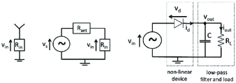
Figure 1: Antenna equivalent circuit (left) and a single diode rectifier (right).

A rectifier is always made of a nonlinear rectifying component such as diode followed by a low pass filter with load [2], [3], [21]-[24] as shown in Fig. 1. The current $i_{d}\left(t\right)$ flowing through an ideal diode (neglecting its series resistance) relates to the voltage drop across the diode $v_{d}\left(t\right)$ = $v_{\mathrm{in}}\left(t\right)$ − $v_{\mathrm{out}}\left(t\right)$ as $i_{d}\left(t\right)=i_{s}\left(e^{\frac{v_{d}\left(t\right)}{nv_{t}}}-1\right)$ where $i_{s}$ is the reverse bias saturation current, $v_{t}$ is the thermal voltage, $n$ is the ideality factor (assumed equal to 1.05). Based on the Taylor expansion of the diode I-V characteristics and some physical assumptions, the analysis of the rectifier circuit is simplified and therefore two simple and tractable models are provided as shown in the following subsections.

III-A Current Model

In [9], by taking the Taylor expansion of the diode I-V characteristics around the negative of the output DC voltage $-v_{\mathrm{out}}$, the output DC current of the rectifier $i_{\mathrm{out}}$ is approximated as

$$i_{\mathrm{out}}\approx k_{0}\left(i_{\mathrm{out}}\right)+\sum_{i\,\mathrm{even},\,i\geq 2}^{n_{0}}k_{i}\left(i_{\mathrm{out}}\right)R_{\mathrm{ant}}^{i/2}\mathscr{\mathcal{E}}\left\{y\left(t\right)^{i}\right\},$$ (5)

where the Taylor expansion is truncated to the $n_{0}$th order term. It is shown that the maximization of $i_{\mathrm{out}}$ is equivalent to maximizing the quantity

$$z_{\mathrm{DC}}=\sum_{i\,\mathrm{even},\,i\geq 2}^{n_{0}}\kappa_{i}\mathscr{\mathcal{E}}\left\{y\left(t\right)^{i}\right\},$$ (6)

where $\kappa_{i}=\frac{i_{s}R_{\mathrm{ant}}^{i/2}}{i!\left(nv_{t}\right)^{i}}$ and $n_{0}=4$ is a good choice [9].

III-B Voltage Model

In [10], by assuming zero output DC current and taking Taylor expansion at zero quiescent point to the $n_{0}$th-order term, the output DC voltage of the rectifier $v_{\mathrm{out}}$ is approximated as

$$v_{\mathrm{out}} =\sum_{i\,\mathrm{even},\,i\geq 2}^{n_{0}}\beta_{i}\mathscr{\mathcal{E}}\left\{y\left(t\right)^{i}\right\},$$ (7)

where $\beta_{i}=\frac{R_{\mathrm{ant}}^{i/2}}{i!\left(nv_{t}\right)^{i-1}}$ and $n_{0}=4$ is a good choice [10]. Multiplying $v_{\mathrm{out}}$ by $\frac{i_{s}}{nv_{t}}$ achieves the same model $z_{\mathrm{DC}}$ (i.e. $\kappa_{i}=\frac{i_{s}}{nv_{t}}\cdot\beta_{i}$) in (6) so those two models are equivalent. In the following Sections, we mainly use the voltage model since it has a straightforward physical meaning. It should be noted that this voltage model is derived based on some simplifications and assumptions (detailed in [10]) so that it can characterize in a simple and tractable manner the dependence of the rectenna nonlinearity on the input signal properties. However, this does not mean that the model in (7) is accurate enough to predict the rectifier output DC power using $P_{\mathrm{out}}=v_{\mathrm{out}}^{2}/R_{L}$ where $R_{L}$ refers to the load resistance. Nevertheless, the model and its benefits in deriving optimized signals have been validated by circuit simulations in [9], [11], [30] and experimentally in [30], [31].

IV Beamforming Optimization with DC Combining

Consider the DC combining scheme for the multiple receive antenna system as shown in Fig. 2. Each receive antenna is connected to a rectifier so that the RF signal received by each antenna is individually rectified. Using the aforementioned voltage model of the nonlinear rectenna, the output DC voltage of the $q$th rectifier (connected to the $q$th receive antenna) is given by

$$v_{\mathrm{out},q} =\sum_{i\,\mathrm{even},\,i\geq 2}^{n_{0}}\beta_{i}\mathscr{\mathcal{E}}\left\{y_{q}\left(t\right)^{i}\right\},$$ (8)

where $\mathscr{\mathcal{E}}\left\{y_{q}\left(t\right)^{i}\right\}$ is given by

$$\mathscr{\mathcal{E}}\left\{y_{q}\left(t\right)^{i}\right\} =\zeta_{i}\left|\mathbf{h}_{q}\mathbf{w}_{T}\right|^{i},$$ (9)

with $\zeta_{i}=\frac{1}{2\pi}\int_{0}^{2\pi}\sin^{i}t\>\textrm{d}t$ and specifically $\zeta_{2}=\frac{1}{2}$, $\zeta_{4}=\frac{3}{8}$, and $\zeta_{6}=\frac{5}{16}$.

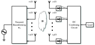
Figure 2: Schematic of the MIMO WPT system with DC combining in the receiver.

The output DC power of all rectifiers are combined together by a DC combining circuit such as multiple-input and multiple-output (MIMO) switching DC-DC converter [32]-[34] as shown in Fig. 2. The total output DC power is then given by $P_{\mathrm{out}}=\sum_{q=1}^{Q}v_{\mathrm{out},q}^{2}/R_{L}$ where we assume each rectifier has the same load $R_{L}$. Therefore, we aim to maximize the total output DC power subject to the transmit power constraint, which can be formulated as

$$\underset{\mathbf{w}_{T}}{\mathrm{max}}\;\;\; \sum_{q=1}^{Q}\frac{v_{\mathrm{out},q}^{2}}{R_{L}}$$ (10)

$$\mathrm{s.t.}\;\;\; \frac{1}{2}\left\|\mathbf{w}_{T}\right\|^{2}\leq P.$$ (11)

Observing the expression of the objective function $P_{\mathrm{out}}$, we find that it is hard to determine whether $P_{\mathrm{out}}$ monotonically increases/decreases with $\Re\left\{w_{T,m}\right\}$ or $\Im\left\{w_{T,m}\right\}$. Hence, we introduce the auxiliary variables $r_{q}=\left|\mathbf{h}_{q}\mathbf{w}_{T}\right|^{2}$ where $r_{q}>0$ and we equivalently rewrite the total output DC power as

$$P_{\mathrm{out}}=\frac{1}{R_{L}}\sum_{q=1}^{Q}\left(\sum_{i\,\mathrm{even},\,i\geq 2}^{n_{0}}\beta_{i}\zeta_{i}r_{q}^{\frac{i}{2}}\right)^{2},$$ (12)

which is a posynomial so that we express it in a compact form that $P_{\mathrm{out}}=\sum_{k=1}^{K}g_{k}\left(\mathbf{r}\right)$ where $K$ is the number of monomials in the posynomial and $g_{k}\left(\mathbf{r}\right)=\rho_{k}r_{1}^{\xi_{1k}}r_{2}^{\xi_{2k}}\cdots r_{Q}^{\xi_{Qk}}$ is the $k$th monomial with $\mathbf{r}=\left[r_{1},r_{2},...r_{Q}\right]^{T}$ where $\xi_{1k}$, …, $\xi_{Qk}$, and $\rho_{k}$ are constants and $\rho_{k}>0$. When $n_{0}=4$ (which is considered in Section VIII), we have $P_{\mathrm{out}}=\frac{1}{R_{L}}\sum_{q=1}^{Q}\left(\beta_{2}^{2}\zeta_{2}^{2}r_{q}^{2}+2\beta_{2}\beta_{4}\zeta_{2}\zeta_{4}r_{q}^{3}+\beta_{4}^{2}\zeta_{4}^{2}r_{q}^{4}\right)$ and there are $K=3Q$ monomials. Therefore, we equivalently rewrite the problem (10)-(11) as

$$\underset{\mathbf{w}_{T},r_{q}}{\mathrm{max}}\;\;\; \sum_{k=1}^{K}g_{k}\left(\mathbf{r}\right)$$ (13)

$$\mathrm{s.t.}\;\;\;\; \frac{1}{2}\left\|\mathbf{w}_{T}\right\|^{2}\leq P,$$ (14)

$$r_{q}=\left|\mathbf{h}_{q}\mathbf{w}_{T}\right|^{2},\>1\leq q\leq Q.$$ (15)

We find that the objective function (13) monotonically increases with $r_{q}$. Hence, the constraint $r_{q}=\left|\mathbf{h}_{q}\mathbf{w}_{T}\right|^{2}$ can be replaced with $r_{q}\leq\left|\mathbf{h}_{q}\mathbf{w}_{T}\right|^{2}$ without affecting the optimal solution of the problem (13)-(15). However, $r_{q}\leq\left|\mathbf{h}_{q}\mathbf{w}_{T}\right|^{2}$ is still a non-convex constraint so we use SDR to transform it to a convex constraint [35]. By introducing an auxiliary positive semi-definite matrix variable $\mathbf{W}_{T}=\mathbf{w}_{T}\mathbf{w}_{T}^{H}$, we equivalently rewrite the problem (13)-(15) as

$$\underset{\mathbf{W}_{T},r_{q}}{\mathrm{max}}\;\;\; \sum_{k=1}^{K}g_{k}\left(\mathbf{r}\right)$$ (16)

$$\mathrm{s.t.}\;\;\;\; \mathrm{Tr}\left(\mathbf{W}_{T}\right)\leq 2P,$$ (17)

$$r_{q}-\mathrm{Tr}\left(\mathbf{h}_{q}^{H}\mathbf{h}_{q}\mathbf{W}_{T}\right)\leq 0,\>1\leq q\leq Q,$$ (18)

$$\mathbf{W}_{T}\succeq 0,$$ (19)

$$\mathrm{rank}\left(\mathbf{W}_{T}\right)=1.$$ (20)

We use SDR to relax the rank-1 constraint (20), but the relaxed problem (16)-(19) is still a non-convex optimization problem. Therefore, we introduce an auxiliary variable $t_{0}>0$ and equivalently rewrite the relaxed problem (16)-(19) as

$$\underset{\mathbf{W}_{T},r_{q},t_{0}}{\mathsf{\mathrm{min}}}\;\;\; \frac{1}{t_{0}}$$ (21)

$$\mathrm{s.t.}\;\;\;\;\;\; \mathrm{Tr}\left(\mathbf{W}_{T}\right)\leq 2P,$$ (22)

$$r_{q}-\mathrm{Tr}\left(\mathbf{h}_{q}^{H}\mathbf{h}_{q}\mathbf{W}_{T}\right)\leq 0,\>1\leq q\leq Q,$$ (23)

$$\mathbf{W}_{T}\succeq 0,$$ (24)

$$\frac{t_{0}}{\sum_{k=1}^{K}g_{k}\left(\mathbf{r}\right)}\leq 1.$$ (25)

However, $1/\sum_{k=1}^{K}g_{k}\left(\mathbf{r}\right)$ is not a posynomial which prevents the transformation to a convex constraint. Therefore, the idea is to upper bound $1/\sum_{k=1}^{K}g_{k}\left(\mathbf{r}\right)$ by a monomial. The choice of the upper bound relies on the fact that an arithmetic mean (AM) is greater or equal to the geometric mean (GM). Hence, we have that

$$\frac{1}{\sum_{k=1}^{K}g_{k}\left(\mathbf{r}\right)}\leq\frac{1}{\prod{}_{k=1}^{K}\left(\frac{g_{k}\left(\mathbf{r}\right)}{\gamma_{k}}\right)^{\gamma_{k}}},$$ (26)

where $\gamma_{k}\geq 0$ and $\sum_{k=1}^{K}\gamma_{k}=1$. We replace the constraint (25) with $t_{0}\prod{}_{k=1}^{K}\left(\frac{g_{k}\left(\mathbf{r}\right)}{\gamma_{k}}\right)^{-\gamma_{k}}\leq 1$ in a conservative way. For a given choice of $\left\{\gamma_{k}\right\}$, the problem (21)-(25) is now replaced by

$$\underset{\mathbf{W}_{T},r_{q},t_{0}}{\mathsf{\mathrm{min}}}\;\;\; \frac{1}{t_{0}}$$ (27)

$$\mathsf{\mathrm{s.t.}}\;\;\;\;\;\; \mathrm{Tr}\left(\mathbf{W}_{T}\right)\leq 2P,$$ (28)

$$r_{q}-\mathrm{Tr}\left(\mathbf{h}_{q}^{H}\mathbf{h}_{q}\mathbf{W}_{T}\right)\leq 0,\>1\leq q\leq Q,$$ (29)

$$\mathbf{W}_{T}\succeq 0,$$ (30)

$$t_{0}\prod{}_{k=1}^{K}\left(\frac{g_{k}\left(\mathbf{r}\right)}{\gamma_{k}}\right)^{-\gamma_{k}}\leq 1,$$ (31)

which looks like a GP problem but actually it is not a standard GP problem because the left sides of the constraints (28), (29), and (30) are not posynomials. To see the details, we rewrite the monomial term as $t_{0}\prod{}_{k=1}^{K}\left(\frac{g_{k}\left(\mathbf{r}\right)}{\gamma_{k}}\right)^{-\gamma_{k}}=c_{1}t_{0}r_{1}^{\alpha_{1}}r_{2}^{\alpha_{2}}\cdots r_{Q}^{\alpha_{Q}}$ where $c_{1}=\prod{}_{k=1}^{K}\left(\frac{\rho_{k}}{\gamma_{k}}\right)^{-\gamma_{k}}$ and $\alpha_{q}=-\sum{}_{k=1}^{K}\xi_{qk}\gamma_{k}$ for $q=1,...,Q$. We introduce auxiliary variables $\tilde{t}_{0}=\log t_{0}$ and $\tilde{r}_{q}=\log r_{q}$ (so that $e^{\tilde{t}_{0}}=t_{0}$ and $e^{\tilde{r}_{q}}=r_{q}$ ). We use the logarithmic transformation for the objective function (27) and the constraints (29) and (31) so we can equivalently rewrite the problem (27)-(31) as

$$\underset{\mathbf{W}_{T},\tilde{r}_{q},\tilde{t}_{0}}{\mathsf{\mathrm{min}}}\;\;\; -\tilde{t}_{0}$$ (32)

$$\mathsf{\mathrm{s.t.}}\;\;\;\;\;\; \mathrm{Tr}\left(\mathbf{W}_{T}\right)\leq 2P,$$ (33)

$$e^{\tilde{r}_{q}}-\mathrm{Tr}\left(\mathbf{h}_{q}^{H}\mathbf{h}_{q}\mathbf{W}_{T}\right)\leq 0,\>1\leq q\leq Q,$$ (34)

$$\mathbf{W}_{T}\succeq 0,$$ (35)

$$\log c_{1}+\tilde{t}_{0}+\sum_{q=1}^{Q}\alpha_{q}\tilde{r}_{q}\leq 0,$$ (36)

which is a convex problem that can be solved within polynomial time by CVX [36] which adopts interior point method.

Note that the tightness of the upper bound (26) heavily depends on the choice of $\left\{\gamma_{k}\right\}$. Following [37], [38], an iterative procedure can be used to tighten the bound, where at each iteration the problem (27)-(31) is solved for an updated set of $\left\{\gamma_{k}\right\}$. Assuming a feasible $\mathbf{r}^{\left(i-1\right)}$ at iteration $i-1$, compute $\gamma_{k}=g_{k}\left(\mathbf{r}^{\left(i-1\right)}\right)/\sum_{k=1}^{K}g_{k}\left(\mathbf{r}^{\left(i-1\right)}\right)\>\forall k$ at iteration $i$ and solve problem (27)-(31) to obtain $\mathbf{r}^{\left(i\right)}$. Repeat the iterations till convergence. Note that the successive approximation method that we used is also known as a successive convex approximation or inner approximation method [39]. It cannot guarantee to converge to the global optimal solution of the problem (21)-(25), but it converges to a stationary point [39], [40] which is denoted as $\mathbf{W}_{T}^{\star}$. Due to the equivalence, $\mathbf{W}_{T}^{\star}$ is also a stationary point of the problem (16)-(19).

If $\mathrm{rank}\left(\mathbf{W}_{T}^{\star}\right)=1$, the SDR is tight so that $\mathbf{W}_{T}^{\star}$ is a stationary point of the problem (16)-(20). Using eigenvalue decomposition (EVD), we obtain $\mathbf{W}_{T}^{\star}=\mathbf{w}_{T}^{\star}\mathbf{w}_{T}^{\star H}$ and therefore $\mathbf{w}_{T}^{\star}$ is a stationary point of the problem (10)-(11). Otherwise, for the case of $\mathrm{rank}\left(\mathbf{W}_{T}^{\star}\right)>1$, we aim to extract a suboptimal rank-1 solution from $\mathbf{W}_{T}^{\star}$. A commonly adopted approach is the so-called Gaussian randomization method [35]. Particularly, we first use the EVD to decompose $\mathbf{W}_{T}^{\star}=\mathbf{U}_{T}\mathbf{\Sigma}_{T}\mathbf{U}_{T}^{H}$ where $\mathbf{U}_{T}$ and $\mathbf{\Sigma}_{T}$ are $M\times M$ unitary and diagonal matrices, respectively. Then, we generate $M$-dimensional random vectors $\mathbf{n}^{\left(l\right)}\sim\mathcal{CN}\left(\mathbf{0},\mathbf{I}\right)$ ($l=1,\ldots,L$), multiply $\mathbf{n}^{\left(l\right)}$ by $\mathbf{U}_{T}\mathbf{\Sigma}_{T}^{1/2}$, and scale the norm of $\mathbf{U}_{T}\mathbf{\Sigma}_{T}^{1/2}\mathbf{n}^{\left(l\right)}$ to $\sqrt{2P}$ ($P$ refers to the transmit power), so that we obtain $\mathbf{w}_{T}^{\left(l\right)}=\sqrt{2P}\frac{\mathbf{U}_{T}\mathbf{\Sigma}_{T}^{1/2}\mathbf{n}^{\left(l\right)}}{\left\|\mathbf{U}_{T}\mathbf{\Sigma}_{T}^{1/2}\mathbf{n}^{\left(l\right)}\right\|}$ ($l=1,\ldots,L$). Finally, we evaluate the output DC power $P_{\mathrm{out}}$ for each $\mathbf{w}_{T}^{\left(l\right)}$ and choose the best one as the final transmit beamforming weight vector $\mathbf{w}_{T}^{\star}$, which has good performance even though it is not guaranteed to be a stationary point of the problem (10)-(11). Algorithm 1 summarizes the procedure for optimizing the beamforming with DC combining. In Section VIII, we numerically show that $\mathbf{W}_{T}^{\star}$ is rank-1 so that Algorithm 1 finds a stationary point of the problem (10)-(11) for all tested channel realizations.

Lastly, it is worth investigating the choice of the truncation order $n_{0}$. Our approach for beamforming optimization with DC combining as shown in Algorithm 1 is applicable to any truncation order $n_{0}$. However, choosing a large truncation order $n_{0}$ is not practical since the optimization complexity exponentially increases with $n_{0}$. In the simplest case $n_{0}=2$, we have that $v_{\mathrm{out},q}=\beta_{2}\mathscr{\mathcal{E}}\left\{y_{q}\left(t\right)^{2}\right\}$. Therefore, in the MISO WPT system (where $Q=1$), truncating to the second order is equivalent to the linear rectenna model [26], [29]. This has also been shown in [9]. However, when it comes to the MIMO WPT system with DC combining, truncating to the second order is not equivalent to the linear rectenna model [26], [29] due to the DC combining operation $\sum_{q=1}^{Q}v_{\mathrm{out},q}^{2}/R_{L}$. On the other hand, it is shown in [9] and [10] that $n_{0}=4$ is a good choice which effectively characterizes the rectenna nonlinearity while the complexity is not high. In Section VII, we show the numerical experimental results of the beamforming optimization with DC combining based on the rectenna model truncated to the 4th order.

1. Initialize: $i=0$, $\mathbf{r}^{\left(0\right)}$, $t_{0}^{\left(0\right)}$

2. do

3. $i=i+1$

4. $\gamma_{k}=g_{k}\left(\mathbf{r}^{\left(i-1\right)}\right)/\sum_{k=1}^{K}g_{k}\left(\mathbf{r}^{\left(i-1\right)}\right)$, $k=1,\ldots,K$

5. Obtain $\mathbf{r}^{\left(i\right)}$, $t_{0}^{\left(i\right)}$, $\mathbf{W}_{T}^{\left(i\right)}$ by solving problem (27)-(31)

6. until $\left|t_{0}^{\left(i\right)}-t_{0}^{\left(i-1\right)}\right|<\epsilon$ or $i=i_{\mathrm{max}}$

7. Set $\mathbf{W}_{T}^{\star}=\mathbf{W}_{T}^{\left(i\right)}$

8. if $\mathrm{rank}\left(\mathbf{W}_{T}^{\star}\right)=1$

9. Obtain $\mathbf{w}_{T}^{\star}$ by $\mathbf{W}_{T}^{\star}=\mathbf{w}_{T}^{\star}\mathbf{w}_{T}^{\star H}$

10. else

11. Obtain $\mathbf{U}_{T}$ and $\mathbf{\Sigma}_{T}$ by $\mathbf{U}_{T}\mathbf{\Sigma}_{T}\mathbf{U}_{T}^{H}=\mathbf{W}_{T}^{\star}$

12. for $l=1$ to $L$ do

13. Generate $\mathbf{n}^{\left(l\right)}\sim\mathcal{CN}\left(\mathbf{0},\mathbf{I}\right)$

14. Obtain $\mathbf{w}_{T}^{\left(l\right)}=\sqrt{2P}\frac{\mathbf{U}_{T}\mathbf{\Sigma}_{T}^{1/2}\mathbf{n}^{\left(l\right)}}{\left\|\mathbf{U}_{T}\mathbf{\Sigma}_{T}^{1/2}\mathbf{n}^{\left(l\right)}\right\|}$

15. end

16. Set $l^{\star}=\underset{l=1,\ldots,L}{\arg\max}\>P_{\mathrm{out}}\left(\mathbf{w}_{T}^{\left(l\right)}\right)$, $\mathbf{w}_{T}^{\star}=\mathbf{w}_{T}^{\left(l^{\star}\right)}$

17. end

Algorithm 1 Beamforming Optimization with DC Combining.

V Beamforming Optimization with RF Combining

Consider the RF combining scheme for the multiple antennas as shown in Fig. 3. All receive antennas are connected to an RF combining circuit. The RF combining circuit includes fixed RF power combiner such as T-junction and reconfigurable power combiner with variable power ratio and phase shifts [41] to adapt to the channel. The received signal at all receive antennas are combined together so that the RF combined signal $\widetilde{y}\left(t\right)$ can be expressed as

$$\widetilde{y}\left(t\right) =\Re\left\{\mathbf{w}_{R}^{H}\mathbf{H}\mathbf{w}_{T}e^{j\omega_{c}t}\right\},$$ (37)

where $\mathbf{w}_{R}$ denotes the receive beamforming weight vector. Since the RF combining circuit is passive, the output power of the RF combining circuit should be equal or less than the input power, which results in a constraint of $\left\|\mathbf{w}_{R}\right\|^{2}\leq 1$. The RF combined signal $\widetilde{y}\left(t\right)$ is then rectified by the only one rectifier in the RF combining scheme as shown in Fig. 3. Using the aforementioned voltage model of the nonlinear rectenna, the output DC voltage of the one rectifier is given by

$$v_{\mathrm{out}} =\sum_{i\,\mathrm{even},\,i\geq 2}^{n_{0}}\beta_{i}\mathscr{\mathcal{E}}\left\{\widetilde{y}\left(t\right)^{i}\right\},$$ (38)

where $\mathscr{\mathcal{E}}\left\{\widetilde{y}\left(t\right)^{i}\right\}$ is given by

$$\mathscr{\mathcal{E}}\left\{\widetilde{y}\left(t\right)^{i}\right\} =\zeta_{i}\left|\mathbf{w}_{R}^{H}\mathbf{H}\mathbf{w}_{T}\right|^{i},$$ (39)

with $\zeta_{i}=\frac{1}{2\pi}\int_{0}^{2\pi}\sin^{i}t\>\textrm{d}t$ (same as (9)).

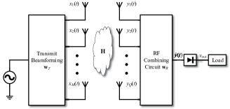
Figure 3: Schematic of the MIMO WPT system with RF combining in the receiver.

We aim to maximize the output DC power $P_{\mathrm{out}}=v_{\mathrm{out}}^{2}/R_{L}$ subject to the transmit power constraint. Noticing that $P_{\mathrm{out}}$ monotonically increases with $\left|\mathbf{w}_{R}^{H}\mathbf{H}\mathbf{w}_{T}\right|^{2}$ irrespectively of the truncation order $n_{0}$, we have the following equivalent problem

$$\underset{\mathbf{w}_{T},\mathbf{w}_{R}}{\mathrm{max}}\;\;\; \left|\mathbf{w}_{R}^{H}\mathbf{H}\mathbf{w}_{T}\right|^{2}$$ (40)

$$\mathsf{\mathrm{s.t.}}\;\;\;\;\; \frac{1}{2}\left\|\mathbf{w}_{T}\right\|^{2}\leq P,$$ (41)

$$\>\>\>\left\|\mathbf{w}_{R}\right\|^{2}\leq 1.$$ (42)

Therefore, the choice of the truncation order $n_{0}$ has no effect on the beamforming optimization with RF combining in the MIMO WPT system, which is different from the case of DC combining.

V-A General Receive Beamforming

The optimal transmit and receive beamforming for the problem (40)-(42) has closed-form solutions by using singular value decomposition (SVD). Using SVD, we can express the channel matrix as $\mathbf{H}=\mathbf{U}\mathbf{\Sigma}\mathbf{V}^{H}$ where $\mathbf{U}$ is a $Q\times Q$ unitary matrix, $\mathbf{V}$ is a $M\times M$ unitary matrix, and $\mathbf{\Sigma}$ is a $Q\times M$ diagonal matrix. Therefore, the optimal transmit and receive beamformers are given by

$$\mathbf{w}_{T}^{\star} =\mathbf{v}_{1}\sqrt{2P},$$ (43)

$$\mathbf{w}_{R}^{\star} =\mathbf{u}_{1},$$ (44)

where $\mathbf{v}_{1}$ and $\mathbf{u}_{1}$ denote the vectors in $\mathbf{V}$ and $\mathbf{U}$ corresponding to the maximum singular value $\sigma_{1}$. Therefore, the maximum value of $\left|\mathbf{w}_{R}^{H}\mathbf{H}\mathbf{w}_{T}\right|^{2}$ is $\sigma_{1}^{2}$.

V-B Analog Receive Beamforming

We consider a practical RF combining circuit for the RF combining scheme as shown in Fig. 4. It consists of an equal-power RF power combiner and $Q$ phase shifters. Each receive antenna is connected to a phase shifter and the outputs of the $Q$ phase shifters are connected to the RF power combiner. Therefore, we refer to it as analog receive beamforming and the analog receive beamforming weight vector satisfies the constraint that

$$\mathbf{w}_{R}=\frac{1}{\sqrt{Q}}\left[e^{-j\theta_{1}},e^{-j\theta_{2}},...,e^{-j\theta_{Q}}\right]^{T},$$ (45)

$$-\pi\leq\theta_{q}<\pi,\>1\leq q\leq Q,$$ (46)

where $\theta_{q}$ denotes the phase shift and the coefficient $\frac{1}{\sqrt{Q}}$ comes from the equal-power RF power combiner (it can be also explained by the constraint $\left\|\mathbf{w}_{R}\right\|^{2}\leq 1$). We replace the constraint (42) with the constraints (45) and (46) so that we have the following problem

$$\underset{\mathbf{w}_{T},\mathbf{w}_{R},\theta_{1},...,\theta_{Q}}{\mathrm{max}} \left|\mathbf{w}_{R}^{H}\mathbf{H}\mathbf{w}_{T}\right|^{2}$$ (47)

$$\mathrm{s.t.}\;\;\quad\; \frac{1}{2}\left\|\mathbf{w}_{T}\right\|^{2}\leq P,$$ (48)

$$\mathbf{w}_{R}=\frac{1}{\sqrt{Q}}\left[e^{-j\theta_{1}},e^{-j\theta_{2}},...,e^{-j\theta_{Q}}\right]^{T},$$ (49)

$$-\pi\leq\theta_{q}<\pi,\>1\leq q\leq Q,$$ (50)

which is a non-convex optimization problem due to the non-convex constraint of $\mathbf{w}_{R}$ (49) and (50). The problem (47)-(50) can be solved by the following two stages.

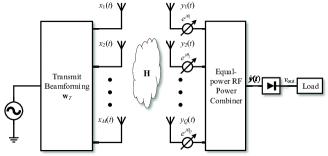
Figure 4: Schematic of the MIMO WPT system with analog receive beamforming in the receiver.

V-B1 Maximum Ratio Transmission

In the first stage, for any given $\mathbf{w}_{R}$, it is known that the maximum ratio transmission (MRT), $\mathbf{w}_{T}=\sqrt{2P}\frac{\left(\mathbf{w}_{R}^{H}\mathbf{H}\right)^{H}}{\left\|\mathbf{w}_{R}^{H}\mathbf{H}\right\|}$, is the optimal transmit beamforming solution so that we have $\left|\mathbf{w}_{R}^{H}\mathbf{H}\mathbf{w}_{T}\right|^{2}=2P\left\|\mathbf{w}_{R}^{H}\mathbf{H}\right\|^{2}$ and the problem (47)-(50) can be equivalently rewritten as

$$\underset{\mathbf{w}_{R},\theta_{1},...,\theta_{Q}}{\mathrm{max}} \left\|\mathbf{w}_{R}^{H}\mathbf{H}\right\|^{2}$$ (51)

$$\mathsf{\mathrm{s.t.}}\;\quad \mathbf{w}_{R}=\frac{1}{\sqrt{Q}}\left[e^{-j\theta_{1}},e^{-j\theta_{2}},...,e^{-j\theta_{Q}}\right]^{T},$$ (52)

$$-\pi\leq\theta_{q}<\pi,\>1\leq q\leq Q,$$ (53)

which is still a non-convex optimization problem due to the non-convex constraints (52), (53).

V-B2 Semi-definite Relaxation

In the second stage, the non-convex constraints (52) and (53) are transformed into convex constraints by using SDR. By introducing an auxiliary positive semi-definite matrix variable $\mathbf{W}_{R}=\mathbf{w}_{R}\mathbf{w}_{R}^{H}$, the problem (51)-(53) is equivalently rewritten as

$$\underset{\mathbf{W}_{R}}{\mathrm{max}}\;\;\; \mathrm{Tr}\left(\mathbf{H}\mathbf{H}^{H}\mathbf{W}_{R}\right)$$ (54)

$$\mathsf{\mathrm{s.t.}}\;\;\; \left[\mathbf{W}_{R}\right]_{qq}=\frac{1}{Q},\>1\leq q\leq Q,$$ (55)

$$\mathbf{W}_{R}\succeq 0,$$ (56)

$$\mathrm{rank}\left(\mathbf{W}_{R}\right)=1.$$ (57)

We use SDR to relax the rank-1 constraint (57) so that the relaxed problem (54)-(56) becomes a semi-definite program (SDP), which can be solved by CVX with complexity of $\mathcal{O}\left(Q^{4.5}\log\frac{1}{\epsilon}\right)$ ($\epsilon$ is the solution accuracy) [35] to achieve the global optimal solution. We denote $\mathbf{W}_{R}^{\star}$ as the global optimal solution of the problem (54)-(56). If $\mathrm{rank}\left(\mathbf{W}_{R}^{\star}\right)=1$, the SDR is tight so that $\mathbf{W}_{R}^{\star}$ is also the global optimal solution of the problem (54)-(57). Using EVD, we obtain $\mathbf{W}_{R}^{\star}=\mathbf{w}_{R}^{\star}\mathbf{w}_{R}^{\star H}$ and therefore $\mathbf{w}_{R}^{\star}$ is the global optimal solution of the problem (51)-(53). Otherwise, for the case of $\mathrm{rank}\left(\mathbf{W}_{R}^{\star}\right)>1$, we aim to extract a suboptimal rank-1 solution from $\mathbf{W}_{R}^{\star}$ by the Gaussian randomization method as shown in Section IV. Particularly, we first use the EVD to decompose $\mathbf{W}_{R}^{\star}=\mathbf{U}_{R}\mathbf{\Sigma}_{R}\mathbf{U}_{R}^{H}$ where $\mathbf{U}_{R}$ and $\mathbf{\Sigma}_{R}$ are $Q\times Q$ unitary and diagonal matrices, respectively. Then, we generate $Q$-dimensional random vectors $\mathbf{n}^{\left(l\right)}\sim\mathcal{CN}\left(\mathbf{0},\mathbf{I}\right)$ ($l=1,\ldots,L$), multiply $\mathbf{n}^{\left(l\right)}$ by $\mathbf{U}_{R}\mathbf{\Sigma}_{R}^{1/2}$, and extract its phase as the phase shift so that we obtain $\mathbf{w}_{R}^{\left(l\right)}=\frac{1}{\sqrt{Q}}e^{j\arg\left(\mathbf{U}_{R}\mathbf{\Sigma}_{R}^{1/2}\mathbf{n}^{\left(l\right)}\right)}$ ($l=1,\ldots,L$). Finally, we evaluate $\left\|\mathbf{w}_{R}^{\left(l\right)H}\mathbf{H}\right\|^{2}$ for each $\mathbf{w}_{R}^{\left(l\right)}$ and choose the best one as the final receive beamforming weight vector $\mathbf{w}_{R}^{\star}$. The Gaussian randomization method guarantees at least a $\frac{\pi}{4}$-approximation of the optimal objective value for the problem (51)-(53) [35]. Once we obtain $\mathbf{w}_{R}^{\star}$, the optimal transmit beamforming weight vector $\mathbf{w}_{T}^{\star}$ can be found by the aforementioned MRT. Algorithm 2 summarizes the procedure for optimizing the analog receive beamforming. In Section VIII, we numerically show that $\mathbf{W}_{R}^{\star}$ is rank-1 matrix for most of the tested channel realizations and therefore Algorithm 2 finds nearly the global optimal solution of the problem (51)-(53) for the tested channel realizations.

1. Obtain $\mathbf{W}_{R}^{\star}$ by solving problem (54)-(57)

2. if $\mathrm{rank}\left(\mathbf{W}_{R}^{\star}\right)=1$

3. Obtain $\mathbf{w}_{R}^{\star}$ by $\mathbf{W}_{R}^{\star}=\mathbf{w}_{R}^{\star}\mathbf{w}_{R}^{\star H}$

4. else

5. Obtain $\mathbf{U}_{R}$ and $\mathbf{\Sigma}_{R}$ by $\mathbf{U}_{R}\mathbf{\Sigma}_{R}\mathbf{U}_{R}^{H}=\mathbf{W}_{R}^{\star}$

6. for $l=1$ to $L$ do

7. Generate $\mathbf{n}^{\left(l\right)}\sim\mathcal{CN}\left(\mathbf{0},\mathbf{I}\right)$

8. Obtain $\mathbf{w}_{R}^{\left(l\right)}=\frac{1}{\sqrt{Q}}e^{j\arg\left(\mathbf{U}_{R}\mathbf{\Sigma}_{R}^{1/2}\mathbf{n}^{\left(l\right)}\right)}$

9. end

10. Set $l^{\star}=\underset{l=1,\ldots,L}{\arg\max}\>\left\|\mathbf{w}_{R}^{\left(l\right)H}\mathbf{H}\right\|^{2}$, $\mathbf{w}_{R}^{\star}=\mathbf{w}_{R}^{\left(l^{\star}\right)}$

11. end

12. Set $\mathbf{w}_{T}^{\star}=\sqrt{2P}\frac{\left(\mathbf{w}_{R}^{\star H}\mathbf{H}\right)^{H}}{\left\|\mathbf{w}_{R}^{\star H}\mathbf{H}\right\|}$

Algorithm 2 Beamforming Optimization with RF Combining.

VI Beneficial Role of Rectenna Nonlinearity

In this section, we provide some insights into the role of nonlinearity. This is crucial to understand why RF combining outperforms DC combining in the output DC power level. The voltage model $v_{\mathrm{out}}=\sum_{i\,\mathrm{even},\,i\geq 2}^{n_{0}}\beta_{i}\mathscr{\mathcal{E}}\left\{y\left(t\right)^{i}\right\}$ characterizes the rectenna nonlinearity which is crucial in WPT system. Using Jensen’s inequality, we have $\mathscr{\mathcal{E}}\left\{y\left(t\right)^{i}\right\}\geq\left(\mathscr{\mathcal{E}}\left\{y\left(t\right)^{2}\right\}\right)^{\frac{i}{2}}=\left(P_{\mathrm{RF}}\right)^{\frac{i}{2}}$ ($P_{\mathrm{RF}}$ is the input RF power) for $i$ is even and $i\geq 2$ so that $v_{\mathrm{out}}\geq\sum_{i\,\mathrm{even},\,i\geq 2}^{n_{0}}\beta_{i}\left(P_{\mathrm{RF}}\right)^{\frac{i}{2}}$, which implies that the RF-to-DC efficiency increases with the input RF power. This is consistent with the measured RF-to-DC efficiency of rectifier circuits in [21]-[24], [30].

To understand the beneficial role of rectenna nonlinearity, we first consider the MIMO WPT system with linear rectenna model which has a constant RF-to-DC conversion efficiency $\eta$. In DC combining, the RF power received by the $q$th antenna is $P_{\mathrm{RF},q}=\frac{1}{2}\left|\mathbf{h}_{q}\mathbf{w}_{T}\right|^{2}$. Each receive antenna is connected to a rectifier so that the output DC power at the $q$th rectifier is given by $P_{\mathrm{out},q}=\frac{1}{2}\left|\mathbf{h}_{q}\mathbf{w}_{T}\right|^{2}\eta$. Therefore, the total output DC power is given by $P_{\mathrm{out}}^{\mathrm{DC\>Combining}}=\frac{1}{2}\left\|\mathbf{H}\mathbf{w}_{T}\right\|^{2}\eta$ where $\mathbf{H}=\left[\mathbf{h}_{1}^{T},\mathbf{h}_{2}^{T},...,\mathbf{h}_{Q}^{T}\right]^{T}$. On the other hand, in RF combining, the RF power of the combined RF signal is $P_{\mathrm{RF}}=\frac{1}{2}\left|\mathbf{w}_{R}^{H}\mathbf{H}\mathbf{w}_{T}\right|^{2}$. The combined RF signal is input into the single rectifier so that the output DC power is given by $P_{\mathrm{out}}^{\mathrm{RF\>Combining}}=\frac{1}{2}\left|\mathbf{w}_{R}^{H}\mathbf{H}\mathbf{w}_{T}\right|^{2}\eta$. It is obvious that the optimal receive beamforming is $\mathbf{w}_{R}^{\star}=\frac{\mathbf{H}\mathbf{w}_{T}}{\left\|\mathbf{H}\mathbf{w}_{T}\right\|}$ so that we have $P_{\mathrm{out}}^{\mathrm{RF\>Combining}}=\frac{1}{2}\left\|\mathbf{H}\mathbf{w}_{T}\right\|^{2}\eta$ which is equal to the total output DC power in DC Combining. Therefore, if we use the linear rectenna model, RF combining has the same performance as DC combining even though the optimal receive beamforming $\mathbf{w}_{R}^{\star}$ is used in RF combining.

However, rectenna is a nonlinear device and the rectenna nonlinearity cannot be ignored. The RF-to-DC conversion efficiency $\eta$ is a function of the input signal waveform and the input power level. For single-tone input signal, $\eta$ increases with the input RF power level, which is denoted as $\eta\left(P_{\mathrm{RF}}\right)$. Considering the rectenna nonlinearity, the total output DC power of DC and RF combining will be different. In DC combining, the output DC power is given by

$$P_{\mathrm{out}}^{\mathrm{DC\>Combining}}=\frac{1}{2}\sum_{q=1}^{Q}\left|\mathbf{h}_{q}\mathbf{w}_{T}\right|^{2}\eta\left(\frac{1}{2}\left|\mathbf{h}_{q}\mathbf{w}_{T}\right|^{2}\right),$$ (58)

where $\eta\left(\frac{1}{2}\left|\mathbf{h}_{q}\mathbf{w}_{T}\right|^{2}\right)$ denotes the RF-to-DC efficiency at the input RF power level of $\frac{1}{2}\left|\mathbf{h}_{q}\mathbf{w}_{T}\right|^{2}$. Therefore, nonlinearity exists in DC combining so that it can be leveraged to increase the output DC power. On the other hand, in RF combining, the output DC power is given by $P_{\mathrm{out}}^{\mathrm{RF\>Combining}}=\frac{1}{2}\left|\mathbf{w}_{R}^{H}\mathbf{H}\mathbf{w}_{T}\right|^{2}\eta\left(\frac{1}{2}\left|\mathbf{w}_{R}^{H}\mathbf{H}\mathbf{w}_{T}\right|^{2}\right)$ where $\eta\left(\frac{1}{2}\left|\mathbf{w}_{R}^{H}\mathbf{H}\mathbf{w}_{T}\right|^{2}\right)$denotes the RF-to-DC efficiency at the input RF power level of $\frac{1}{2}\left|\mathbf{w}_{R}^{H}\mathbf{H}\mathbf{w}_{T}\right|^{2}$. The optimal receive beamforming is still $\mathbf{w}_{R}^{\star}=\frac{\mathbf{H}\mathbf{w}_{T}}{\left\|\mathbf{H}\mathbf{w}_{T}\right\|}$ which simultaneously maximize the terms $\left|\mathbf{w}_{R}^{H}\mathbf{H}\mathbf{w}_{T}\right|^{2}$ and $\eta\left(\frac{1}{2}\left|\mathbf{w}_{R}^{H}\mathbf{H}\mathbf{w}_{T}\right|^{2}\right)$. Then, the output DC power with $\mathbf{w}_{R}^{\star}$ is given by

$$P_{\mathrm{out}}^{\mathrm{RF\>Combining}}=\frac{1}{2}\left\|\mathbf{H}\mathbf{w}_{T}\right\|^{2}\eta\left(\frac{1}{2}\left\|\mathbf{H}\mathbf{w}_{T}\right\|^{2}\right),$$ (59)

which shows that nonlinearity also exists in RF combining so that it can be leveraged. Therefore, we can conclude that rectenna nonlinearity plays a beneficial role in both DC and RF combinings to increase the output DC power. However, the receive beamforming in RF combining can leverage the nonlinearity more efficiently than DC combining which has no receive beamforming. In DC combining, the efficiency for each rectenna is $\eta\left(\frac{1}{2}\left|\mathbf{h}_{q}\mathbf{w}_{T}\right|^{2}\right)$ while in RF combining the efficiency is $\eta\left(\frac{1}{2}\left\|\mathbf{H}\mathbf{w}_{T}\right\|^{2}\right)$. Since the efficiency increases with the input RF power, we have $\eta\left(\frac{1}{2}\left\|\mathbf{H}\mathbf{w}_{T}\right\|^{2}\right)\geq\eta\left(\frac{1}{2}\left|\mathbf{h}_{q}\mathbf{w}_{T}\right|^{2}\right)$ so that $P_{\mathrm{out}}^{\mathrm{RF\>Combining}}\geq P_{\mathrm{out}}^{\mathrm{DC\>Combining}}$. Hence, we can conclude that RF combining outperforms DC combining because the receive beamforming in RF combining can leverage the nonlinearity more efficiently than DC combining. This conclusion is also verified in the next sections of scaling laws analysis and performance evaluations.

VII Scaling Laws

In order to get insights into the fundamental limits of MIMO WPT system and get insights into the role of the combining strategy, we want to quantify how the output DC power $P_{\mathrm{out}}$ scales as a function of the number of transmit antennas $M$ and the number of receive antennas $Q$. In the following, we consider MISO WPT system and SIMO WPT system, respectively, and for SIMO WPT system we consider the DC combining and RF combining, respectively. We mainly consider the scaling laws with the truncation order $n_{0}=4$. We assume that the channel gains $h$ are modeled as i.i.d. CSCG random variables with zero mean and unit variance. In this Section, we also assume that $R_{L}=1\;\Omega$ for simplicity.

VII-A MISO WPT System

We first consider the MISO system. Because there is only one antenna at the receiver, there is no combining issue. The output DC voltage of the single rectifier is given by $v_{\mathrm{out}}=\frac{\beta_{2}}{2}\left|\mathbf{h}\mathbf{w}_{T}\right|^{2}+\frac{3\beta_{4}}{8}\left|\mathbf{h}\mathbf{w}_{T}\right|^{4}$ where $\mathbf{h}=\left[h_{1},h_{2},\ldots,h_{M}\right]$ refers to the channel vector (a row vector) for the MISO system. It is obvious that the MRT $\mathbf{w}_{T}=\sqrt{2P}\frac{\mathbf{h}^{H}}{\left\|\mathbf{h}\right\|}$ gives the maximum output DC voltage $v_{\mathrm{out,\>MRT}}=\beta_{2}P\left\|\mathbf{h}\right\|^{2}+\frac{3\beta_{4}P^{2}}{2}\left\|\mathbf{h}\right\|^{4}$ so that we have the maximum output DC power given by $P_{\mathrm{out,\>MRT}}=\beta_{2}^{2}P^{2}\left\|\mathbf{h}\right\|^{4}+3\beta_{2}\beta_{4}P^{3}\left\|\mathbf{h}\right\|^{6}+\frac{9\beta_{4}^{2}P^{4}}{4}\left\|\mathbf{h}\right\|^{8}.$ Therefore, the average output DC power is given by $\bar{P}_{\mathrm{out,\>MRT}}=\>\>\beta_{2}^{2}P^{2}\mathscr{\mathcal{E}}\left\{\left\|\mathbf{h}\right\|^{4}\right\}+3\beta_{2}\beta_{4}P^{3}\mathscr{\mathcal{E}}\left\{\left\|\mathbf{h}\right\|^{6}\right\}+\frac{9\beta_{4}^{2}P^{4}}{4}\mathscr{\mathcal{E}}\left\{\left\|\mathbf{h}\right\|^{8}\right\}.$ Making use of the moments of a $\chi_{2M}^{2}$ random variable, we have that $\mathscr{\mathcal{E}}\left\{\left\|\mathbf{h}\right\|^{2n}\right\}=\frac{\left(M+n-1\right)!}{\left(M-1\right)!}$ so that the average output DC power is given by

$$\bar{P}_{\mathrm{out,\>MRT}}=\> \>\beta_{2}^{2}P^{2}M\left(M+1\right)$$

$$+3\beta_{2}\beta_{4}P^{3}M\left(M+1\right)\left(M+2\right)$$

$$+\frac{9\beta_{4}^{2}P^{4}}{4}M\left(M+1\right)\left(M+2\right)\left(M+3\right).$$ (60)

Equation (60) shows that $\bar{P}_{\mathrm{out,\>MRT}}$ increases with $M$ in the order of $M^{4}$ when the number of transmit antennas $M$ is large, which demonstrates that by adapting to CSI using multiple antennas at the transmitter can effectively increase the output DC power level at the rectenna.

VII-B SIMO WPT System

We then consider the SIMO system. There is no transmit beamforming due to the only one antenna at the transmitter. In the presence of multiple receive antennas, we consider the DC combining and RF combining in the following.

VII-B1 DC Combining

The received signal at the $q$-th receive antenna is given by $y_{q}\left(t\right)=\Re\left\{\sqrt{2P}h_{q}e^{j\omega_{c}t}\right\}$ where $h_{q}$ refers to the channel gain for the $q$-th receive antenna, so that the output DC voltage of the $q$th rectifier is given by $v_{\mathrm{out},q}^{\mathrm{DC\>Combining}}=\beta_{2}P\left|h_{q}\right|^{2}+\frac{3\beta_{4}P^{2}}{2}\left|h_{q}\right|^{4}.$The total output DC power is given by $P_{\mathrm{out}}^{\mathrm{DC\>Combining}}=\sum_{q=1}^{Q}\left(\beta_{2}^{2}P^{2}\left|h_{q}\right|^{4}+3\beta_{2}\beta_{4}P^{3}\left|h_{q}\right|^{6}+\frac{9\beta_{4}^{2}P^{4}}{4}\left|h_{q}\right|^{8}\right).$ Therefore we can find the average total output DC power, which is given by $\bar{P}_{\mathrm{out}}^{\mathrm{DC\>Combining}}=\sum_{q=1}^{Q}(\beta_{2}^{2}P^{2}\mathscr{\mathcal{E}}\left\{\left|h_{q}\right|^{4}\right\}+3\beta_{2}\beta_{4}P^{3}\mathscr{\mathcal{E}}\left\{\left|h_{q}\right|^{6}\right\}+\frac{9\beta_{4}^{2}P^{4}}{4}\mathscr{\mathcal{E}}\left\{\left|h_{q}\right|^{8}\right\}).$ Making use of the moments of the exponential distribution, we have $\mathscr{\mathcal{E}}\left\{\left|h_{q}\right|^{4}\right\}=2$, $\mathscr{\mathcal{E}}\left\{\left|h_{q}\right|^{6}\right\}=6$, $\mathscr{\mathcal{E}}\left\{\left|h_{q}\right|^{8}\right\}=24$, so that the average output DC power is given by

$$\bar{P}_{\mathrm{out}}^{\mathrm{DC\>Combining}} =\left(2\beta_{2}^{2}P^{2}+18\beta_{2}\beta_{4}P^{3}+54\beta_{4}^{2}P^{4}\right)Q,$$ (61)

which shows that $\bar{P}_{\mathrm{out}}^{\mathrm{DC\>Combining}}$ linearly increases with $Q$.

VII-B2 RF Combining

The RF combined signal is $\widetilde{y}\left(t\right)=\Re\left\{\sqrt{2P}\mathbf{w}_{R}^{H}\mathbf{h}e^{j\omega_{c}t}\right\}$ where $\mathbf{h}=\left[h_{1},h_{2},\ldots,h_{Q}\right]^{T}$ refers to the SIMO channel vector. The output DC voltage of the single rectifier is given by $v_{\mathrm{out}}^{\mathrm{RF\>Combining}}=\beta_{2}P\left|\mathbf{w}_{R}^{H}\mathbf{h}\right|^{2}+\frac{3\beta_{4}P^{2}}{2}\left|\mathbf{w}_{R}^{H}\mathbf{h}\right|^{4}.$ It is obvious that the maximum ratio combining (MRC) $\mathbf{w}_{R}=\frac{\mathbf{h}}{\left\|\mathbf{h}\right\|}$ gives the maximum output DC voltage $v_{\mathrm{out,\>MRC}}^{\mathrm{RF\>Combining}}=\beta_{2}P\left\|\mathbf{h}\right\|^{2}+\frac{3\beta_{4}P^{2}}{2}\left\|\mathbf{h}\right\|^{4}.$ Similar to the MISO WPT case, the average output DC power in this case is given by

$$\bar{P}_{\mathrm{out,\>MRC}}^{\mathrm{RF\>Combining}}=\> \>\beta_{2}^{2}P^{2}Q\left(Q+1\right)$$

$$+3\beta_{2}\beta_{4}P^{3}Q\left(Q+1\right)\left(Q+2\right)$$

$$+\frac{9\beta_{4}^{2}P^{4}}{4}Q\left(Q+1\right)\left(Q+2\right)\left(Q+3\right),$$ (62)

which shows that the average output DC power $\bar{P}_{\mathrm{out,\>MRC}}^{\mathrm{RF\>Combining}}$ increases with $Q$ in the order of $Q^{4}$ when the number of receive antennas $Q$ is large.

Now we consider the analog receive beamforming where the receive beamforming weight is constrained by (45), (46). It is obvious that the optimal analog receive beamforming weight is $\mathbf{w}_{R}=\frac{1}{\sqrt{Q}}e^{j\arg\left(\mathbf{h}\right)}$ so that the output DC voltage is given by $v_{\mathrm{out,\>Analog}}^{\mathrm{RF\>Combining}}=\beta_{2}P\frac{\left\|\mathbf{h}\right\|_{1}^{2}}{Q}+\frac{3\beta_{4}P^{2}}{2}\frac{\left\|\mathbf{h}\right\|_{1}^{4}}{Q^{2}}.$ Therefore, the average output DC power is given by

$$\bar{P}_{\mathrm{out,\>Analog}}^{\mathrm{RF\>Combining}}=\> \>\beta_{2}^{2}P^{2}\frac{\mathscr{\mathcal{E}}\left\{\left\|\mathbf{h}\right\|_{1}^{4}\right\}}{Q^{2}}+3\beta_{2}\beta_{4}P^{3}\frac{\mathscr{\mathcal{E}}\left\{\left\|\mathbf{h}\right\|_{1}^{6}\right\}}{Q^{3}}$$

$$+\frac{9\beta_{4}^{2}P^{4}}{4}\frac{\mathscr{\mathcal{E}}\left\{\left\|\mathbf{h}\right\|_{1}^{8}\right\}}{Q^{4}}.$$ (63)

Finding the closed-form expressions of the moments of random variable $\left\|\mathbf{h}\right\|_{1}$ is complicated. For simplicity, we give a tight lower bound (for large $Q$) as $\mathscr{\mathcal{E}}\left\{\left\|\mathbf{h}\right\|_{1}^{n}\right\}\geq\frac{Q!}{\left(Q-n\right)!}\mathscr{\mathcal{E}}\left\{\left|h_{q}\right|\right\}^{n}=\frac{Q!}{\left(Q-n\right)!}\Gamma\left(1.5\right)^{n}$ where $\Gamma(x)$ refers to the gamma function. Therefore, we have the lower bound for the average output DC power as

$$\bar{P}_{\mathrm{out,\>Analog}}^{\mathrm{RF\>Combining}}\geq\> \>\frac{\beta_{2}^{2}P^{2}\Gamma\left(1.5\right)^{4}Q!}{Q^{2}\left(Q-4\right)!}+\frac{3\beta_{2}\beta_{4}P^{3}\Gamma\left(1.5\right)^{6}Q!}{Q^{3}\left(Q-6\right)!}$$

$$+\frac{9\beta_{4}^{2}P^{4}\Gamma\left(1.5\right)^{8}Q!}{4Q^{4}\left(Q-8\right)!},$$ (64)

which shows that the average output DC power $\bar{P}_{\mathrm{out,\>Analog}}^{\mathrm{RF\>Combining}}$ increases with $Q$ in the order of $Q^{4}$ when the number of receive antennas $Q$ is large in spite of the lower bound. We also use Monte Carlo method to find $\bar{P}_{\mathrm{out,\>Analog}}^{\mathrm{RF\>Combining}}$, and compare it with the lower bound in (64) as shown in Fig. 5, which shows that the lower bound in (64) is tight.

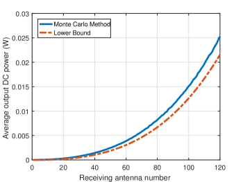
Figure 5: Comparison of $\bar{P}_{\mathrm{out,\>Analog}}^{\mathrm{RF\>Combining}}$ and the lower bound in (64).

To conclude, equation (61) suggests that the average output DC power linearly increases with $Q$ in the DC combining while equation (62) and (64) suggest that the average output DC power increases with $Q$ in the order of $Q^{4}$ for large $Q$ in the RF combining. Therefore, using multiple antennas at the receiver can effectively increase the average output DC power for both combinings, but the RF combining outperforms the DC combining since the receive beamforming in RF combining leverages the rectenna nonlinearity more efficiently than DC combining which has no receive beamforming (see Section VI).

Compared with the MRT MISO WPT system (60), the SIMO WPT system using the MRC RF combining can achieve the same scaling law (62) while using the analog receive beamforming achieves a slightly lower (but same order) scaling law (64). Besides, the SIMO WPT system with DC combining (61) achieves a much lower scaling law than the MRT MISO WPT system. Therefore, overall the MISO WPT system is more beneficial than the SIMO system. However, using the MIMO WPT system can simultaneously exploit the benefits of MISO and SIMO system to boost the output DC power.

Table I summarizes the scaling laws for MISO and SIMO systems with DC and RF combinings. The scaling laws for MISO and SIMO systems with DC and RF combinings for $n_{0}=2$ are also provided in Table I. Interestingly, the scaling laws for $n_{0}=2$ can be easily derived from the scaling laws for $n_{0}=4$ by setting $\beta_{4}=0$. We notice that the scaling laws change with the truncation order. For example, in MISO WPT system the average output DC power increases with $M$ in the order of $M^{2}$, instead of $M^{4}$, for large $M$. In addition, RF combining still outperforms the DC combining because $n_{0}=2$ is not equivalent to the linear model in MIMO WPT system with DC combining as discussed in Section IV.

TABLE I: Summary of Scaling Laws

Beamforming	$M$, $Q$	$n_{0}=2$	$n_{0}=4$
MISO
$\bar{P}_{\mathrm{out,\>MRT}}$	$M\geq 1$, $Q=1$	$\beta_{2}^{2}P^{2}M\left(M+1\right)$	$\beta_{2}^{2}P^{2}M\left(M+1\right)+3\beta_{2}\beta_{4}P^{3}M\left(M+1\right)\left(M+2\right)+\frac{9\beta_{4}^{2}P^{4}}{4}M\left(M+1\right)\left(M+2\right)\left(M+3\right)$
SIMO
$\bar{P}_{\mathrm{out}}^{\mathrm{DC\>Combining}}$	$M=1$, $Q\geq 1$	$2\beta_{2}^{2}P^{2}Q$	$\left(2\beta_{2}^{2}P^{2}+18\beta_{2}\beta_{4}P^{3}+54\beta_{4}^{2}P^{4}\right)Q$
$\bar{P}_{\mathrm{out,\>MRC}}^{\mathrm{RF\>Combining}}$	$M=1$, $Q\geq 1$	$\beta_{2}^{2}P^{2}Q\left(Q+1\right)$	$\beta_{2}^{2}P^{2}Q\left(Q+1\right)+3\beta_{2}\beta_{4}P^{3}Q\left(Q+1\right)\left(Q+2\right)+\frac{9\beta_{4}^{2}P^{4}}{4}Q\left(Q+1\right)\left(Q+2\right)\left(Q+3\right)$
$\bar{P}_{\mathrm{out,\>Analog}}^{\mathrm{RF\>Combining}}$	$M=1$, $Q\geq 1$	$\geq\frac{\beta_{2}^{2}P^{2}\Gamma\left(1.5\right)^{4}Q!}{Q^{2}\left(Q-4\right)!}$	$\geq\frac{\beta_{2}^{2}P^{2}\Gamma\left(1.5\right)^{4}Q!}{Q^{2}\left(Q-4\right)!}+\frac{3\beta_{2}\beta_{4}P^{3}\Gamma\left(1.5\right)^{6}Q!}{Q^{3}\left(Q-6\right)!}+\frac{9\beta_{4}^{2}P^{4}\Gamma\left(1.5\right)^{8}Q!}{4Q^{4}\left(Q-8\right)!}$

VIII Performance Evaluations

We consider two types of performance evaluations, the first one is based on the simplified and tractable nonlinear rectenna model truncated to the 4th order as introduced in Section III, while the second one relies on an actual and accurate modeling of the rectenna in the circuit simulation solver Advanced Design System (ADS).

VIII-A Nonlinear Model-Based Performance Evaluations

The first type of evaluations displays $P_{\mathrm{out}}$ averaged over many channel realizations for DC and RF combinings. We assume $v_{t}=25.86$ mV, $n=1.05$, and $R_{L}=5000\;\Omega$.

We now evaluate the performance of the MIMO WPT system with DC and RF combinings in a scenario representative of a WiFi-like environment at a center frequency of 2.45 GHz with a 36 dBm transmit power and 66 dB path loss with a Rayleigh fading. The elements of the channel matrix $\mathbf{H}$ are modeled as i.i.d. circularly symmetric complex Gaussian random variables and the average received power is -30 dBm.

For DC combining, we evaluate the adaptive optimized (OPT) transmit beamforming as shown in Algorithm 1 versus a benchmark: a transmit beamforming scheme based on SVD. Specially, such transmit beamforming weight vector is given by $\mathbf{w}_{T}=\mathbf{v}_{1}\sqrt{2P}$ which is the same as (43) in that $\mathbf{v}_{1}$ denotes the vector in $\mathbf{V}$ corresponding to the maximum singular value $\sigma_{1}$ and $\mathbf{V}$ is obtained from SVD $\mathbf{H}=\mathbf{U}\mathbf{\Sigma}\mathbf{V}^{H}$. This transmit beamforming is optimal for maximizing the output DC power when the linear model of rectenna is considered [29]. For RF combining, we evaluate the general receive beamforming based on SVD and the analog receive beamforming (ABF) as shown in Algorithm 2. Other baselines for DC and RF combinings have been simulated but we omit them in the paper since they have worse performance than the chosen baselines. We also assume that $L=100$ for the Gaussian randomization method in Algorithm 1 and 2.

Fig. 6 displays the output DC power $P_{\mathrm{out}}$ averaged over many channel realizations versus the number of receive antennas for different numbers of transmit antennas. We make the following observations. First, the output DC power increases with the number of transmit/receive antennas for the four beamformings with DC and RF combinings, showing that the output DC power can be effectively increased by using multiple antennas at the transmitter/receiver. Second, for DC combining, the OPT beamforming achieves higher output DC power than the beamforming based on SVD. This is because the OPT beamforming leverages the rectenna nonlinearity that the RF-to-DC conversion efficiency increases with the input RF power while the beamforming based on SVD ignores the rectenna nonlinearity. Third, for RF combining, the general receive beamforming based on SVD outperforms the analog receive beamforming. This is because the constraints of the analog receive beamforming (45), (46) restrict the received RF power. Fourth, RF combining outperforms DC combining, especially when the number of receive antennas goes large. This is because the receive beamforming in RF combining leverages the rectenna nonlinearity more efficiently by inputting the combined RF signal into a single rectifier (see Section VI). Since the RF-to-DC conversion efficiency increases with the input RF power, RF combining can achieve a higher RF-to-DC conversion efficiency than DC combining which inputs each RF signal to each rectifier, so that RF combinings has a higher output DC power.

To get insights into how the rectenna nonlinearity influences the output DC power, Fig. 7 displays the received RF power averaged over many channels versus the number of receive antennas for different numbers of transmit antennas. We make the following observations. First, the beamforming based on SVD in DC combining has the same received RF power as the beamforming based on SVD in RF combining, which is obvious since they all use the SVD of channel matrix $\mathbf{H}$. Second, for RF combining, the analog receive beamforming has less received RF power than the general receive beamforming based on SVD which is due to the constraints of analog receive beamforming (45), (46). Third, for DC combining, the OPT beamforming has less received RF power than the beamforming based on SVD.

Based on the above observations from Fig. 6 and Fig. 7, we can find that achieving the maximum received RF power does not mean achieving the maximum output DC power due to the rectenna nonlinearity. Therefore, the rectenna nonlinearity should be leveraged in WPT to increase the output DC power. This behavior has been extensively emphasized in [9], [43], but finds further consequences in MIMO WPT. Namely, it is concluded from the simulations that two approaches can be used to leverage the rectenna nonlinearity: 1) optimizing beamforming by considering the rectenna nonlinearity in DC combining, and 2) using RF combining which can leverage the rectenna nonlinearity more efficiently.

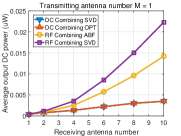
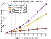
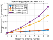
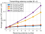
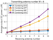
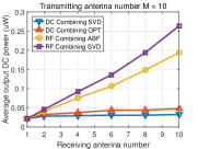
Figure 6: Average output DC power versus the number of receive antennas for different numbers of transmit antennas based on the rectenna model.

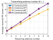
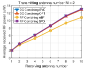
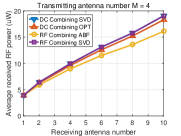
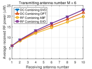
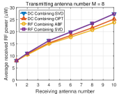
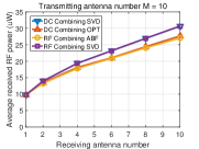
Figure 7: Average received RF power versus the number of receive antennas for different numbers of transmit antennas.

We also evaluate the performance of Algorithms 1 and 2, which both use the technique SDR. For Algorithm 1, we find that $\mathbf{W}_{T}^{\star}$ is rank-1 for all tested channel realizations with different $M$ and $Q$. Hence, Algorithm 1 finds a stationary point of the problem (10)-(11) so its performance is guaranteed for all tested channel realizations. For Algorithm 2, we find that $\mathbf{W}_{R}^{\star}$ is rank-1 for most of the tested channel realizations with different $M$ and $Q$, but not rank-1 for some channel realizations. So, for each channels realization, we compute a quantity $R_{1}=\lambda_{\mathrm{max}}\left(\mathbf{W}_{R}^{\star}\right)/\sum_{q=1}^{Q}\lambda_{q}\left(\mathbf{W}_{R}^{\star}\right)$ where $\lambda_{\mathrm{max}}\left(\mathbf{W}_{R}^{\star}\right)$ is the maximum eigenvalue of $\mathbf{W}_{R}^{\star}$ and $\sum_{q=1}^{Q}\lambda_{q}\left(\mathbf{W}_{R}^{\star}\right)$ is the sum of all the eigenvalues of $\mathbf{W}_{R}^{\star}$. For $\mathbf{W}_{R}^{\star}\succeq 0$, $R_{1}=1$ means $\mathbf{W}_{R}^{\star}$ is rank-1, and heuristically we have that $\mathbf{W}_{R}^{\star}$ is close to rank-1 when $R_{1}$ is close to 1. The average $R_{1}$ over channel realizations, denoted as $\bar{R}_{1}$, are summarized in Table II. We find that $\bar{R}_{1}\geq 0.94$ for different $M$ and $Q$, showing that $\mathbf{W}_{R}^{\star}$ is highly likely to be rank-1. Besides, we also compute a quantity $R_{2}=\mathrm{Tr}\left(\mathbf{H}\mathbf{H}^{H}\mathbf{w}_{R}^{\star}\mathbf{w}_{R}^{\star H}\right)/\mathrm{Tr}\left(\mathbf{H}\mathbf{H}^{H}\mathbf{W}_{R}^{\star}\right)$ which shows how tight the SDR is in the problem (54)-(57). The average $R_{2}$ over channel realizations, denoted as $\bar{R}_{2}$, are also summarized in Table II. We can find that $\bar{R}_{2}\geq 0.997$ for different $M$ and $Q$, showing that the SDR is very tight. So, Algorithm 2 finds nearly the global optimal solution of the problem (54)-(57) and its performance is guaranteed for the tested channel realizations.

TABLE II: Evaluations of Algorithm 2.

	$Q=1$		$Q=2$		$Q=4$		$Q=6$		$Q=8$		$Q=10$
	$\bar{R}_{1}$	$\bar{R}_{2}$	$\bar{R}_{1}$	$\bar{R}_{2}$	$\bar{R}_{1}$	$\bar{R}_{2}$	$\bar{R}_{1}$	$\bar{R}_{2}$	$\bar{R}_{1}$	$\bar{R}_{2}$	$\bar{R}_{1}$	$\bar{R}_{2}$
$M=1$	1.0000	1.0000	0.9970	0.9999	0.9991	0.9999	0.9988	0.9999	0.9998	0.9999	0.9993	0.9999
$M=2$	1.0000	1.0000	0.9983	0.9999	0.9976	0.9999	0.9946	0.9999	0.9847	0.9997	0.9716	0.9989
$M=4$	1.0000	1.0000	0.9989	0.9999	0.9975	0.9999	0.9910	0.9999	0.9818	0.9996	0.9681	0.9991
$M=6$	1.0000	1.0000	0.9993	0.9999	0.9969	0.9999	0.9858	0.9999	0.9781	0.9993	0.9470	0.9978
$M=8$	1.0000	1.0000	0.9995	0.9999	0.9974	0.9999	0.9861	0.9999	0.9717	0.9993	0.9524	0.9982
$M=10$	1.0000	1.0000	0.9996	0.9999	0.9972	0.9999	0.9815	0.9996	0.9664	0.9990	0.9482	0.9983

VIII-B Accurate and Realistic Performance Evaluations

The second type of evaluations is based on an accurate modeling of the rectenna in ADS in order to validate the beamforming optimization with the two combinings and the rectenna nonlinearity model. To that end, in DC combining the RF signal received by each receive antenna is used as input to a realistic rectenna as shown in Fig. 8. Hence $Q$ rectifiers as shown in Fig. 8 are used. While in RF combining, only one rectifier as shown in Fig. 8 is used. The rectenna circuit contains a voltage source, an antenna impedance, an L-matching network, a Schottky diode SMS-7630, a capacitor as low-pass filter, and a load resistor. The L-matching network is used to guarantee a good matching between the rectifier and the antenna and to minimize the impedance mismatch due to variations in input RF power level. By using the Harmonic Balance solver with the SPICE model of SMS-7630 in ADS, the values of the capacitor $C_{1}$ and the inductor $L_{1}$ in the matching network are optimized to achieve a good impedance matching.

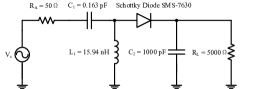
Figure 8: Rectenna with a single diode and L-matching network used for circuit evaluation in ADS.

We now evaluate the performance of the MIMO WPT system with DC and RF combinings using the accurate modeling of rectenna in ADS. Again, we consider two DC combinings (based on SVD and OPT) and two RF combinings (based on ABF and SVD). Fig. 9 displays the average (over many channel realizations) output DC power solved by ADS versus the number of receive antennas for different numbers of transmit antennas. Similar to Fig. 6, we can make the following observations. First, the output DC power increases with the number of transmit/receive antennas in both DC and RF combinings. Second, for DC combining, the OPT beamforming achieves higher output DC power than the beamforming based on SVD. Third, for RF combining, the general receive beamforming based on SVD outperforms the analog receive beamforming. Fourth, RF combinings lead to higher average output DC power than DC combining, especially when the number of receive antennas goes large. The relative gain of RF combining versus DC combining can exceed 100% when the receive antenna number is larger than 6, and it can reach 240% (achieved when there is a single transmit antenna and 10 receive antennas). The explanations for these observations can be found in the above evaluations. Therefore, the similar observations in Fig. 6 and Fig. 9 confirm the usefulness of the rectenna nonlinearity model and demonstrate the necessity of leveraging the rectenna nonlinearity in WPT to boost the output DC power.

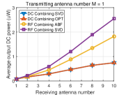
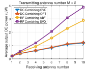
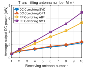
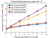
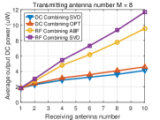
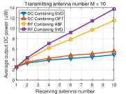
Figure 9: Average output DC power versus the number of receive antennas for different numbers of transmit antennas based on the accurate and realistic circuit simulation.

IX Discussions

In addition to evaluating the performance of DC combining versus RF combining in MIMO WPT system, it is also worth discussing the impact of DC combining versus RF combining on the WPT system design.

IX-A Channel Estimation

DC combining only needs CSIT for transmit beamforming optimization. However, RF combining not only needs CSIT but also need CSIR for joint transmit and receive beamforming optimization. Therefore, channel estimation is required at the receiver for RF combining, which increases the complexity of WPT system design. Alternatively, some forms of communication between the transmitter and the receiver is needed to tell the receiver about the combining weights to use.

IX-B Number of Rectifiers

In DC combining, each receive antenna is connected to a rectifier so that the number of rectifiers increases with the number of receive antennas. However, in RF combining, the RF signals from all receive antennas are firstly RF combined so that only a single rectifier is needed to rectify the combined RF signal.

IX-C Combining Network

DC combining does not need a RF combining circuit. Instead, it needs a good DC combining circuit such as MIMO switching DC-DC converter [32]-[34]. Because the RF power input into each rectifier is different in the MIMO WPT system, the optimal DC bias voltage for maximizing the RF-to-DC efficiency is different for each rectifier. The MIMO switching DC-DC converter provides the optimal DC bias voltage for each rectifier so that the output DC power of all rectifiers can be efficiently combined. However, using the MIMO switching DC-DC converter increases the complexity of WPT system design. On the other hand, RF combining only needs a simple single-input and single-output (SISO) switching DC-DC converter, but RF combining needs a RF combining circuit to combine all the received RF signal. The proposed analog receive beamforming consists of multiple phase shifters and a RF power combiner, and the number of phase shifters increases with the number of receive antennas.

A comprehensive comparison of DC combining and RF combining is shown in Table. III. We can conclude that RF combining achieves high output DC power at the cost of CSIT and CSIR and RF combining circuit while DC combining is limited by the low output DC power, multiple rectifiers, and MIMO DC-DC converter but it only needs CSIT and it does not need a RF combining circuit.

X Conclusion and Future Works

In this paper, we propose a MIMO WPT architecture where the transmitter and the receiver are equipped with multiple antennas, so as to enhance the output DC power level. Two combining strategies at the receiver are introduced, namely DC and RF combining, and the corresponding beamformers are optimized considering the rectenna nonlinearity.

For DC combining, assuming perfect CSIT and using the rectenna nonlinearity model, the beamforming for multiple antennas at the transmitter adaptive to CSI is optimized to maximize the output DC power by solving a non-convex posynomial maximization problem with SDR. It is also numerically shown that the proposed algorithm can find a stationary point of the problem for the tested channel realizations.

TABLE III: Comprehensive Comparison of DC Combining and RF Combining

	DC combining	RF combining
Output DC power	low	high
Channel estimation	CSIT	CSIT and CSIR
Number of rectifiers	Multiple	Single
DC-DC converter	MIMO	SISO
RF Combining Circuit	No need	Need

For RF combining, assuming perfect CSIT and CSIR and using the rectenna nonlinearity model, the beamforming for multiple antennas at both the transmitter and receiver adaptive to CSI is optimized for output DC power maximization. The global optimal transmit and receive beamforming are obtained in closed form. In addition, we propose a practical RF combining circuit using RF phase shifter and RF power combiner and also optimize the analog receive beamforming adaptive to CSI by solving a non-convex optimization problem with SDR. It is also numerically shown that the proposed algorithm can find nearly the global optimal solution of the problem for the tested channel realizations.

We also analytically derive the scaling laws of the output DC power for MISO and SIMO systems with DC and RF combinings as a function of the number of transmit and receive antennas. Those scaling laws highlight the benefits of using multiple antennas at the transmitter and the receiver. They also highlight the benefits of using RF combining over DC combining since the receive beamforming in RF combining leverages the rectenna nonlinearity more efficiently.

We also provide two types of performance evaluations for DC and RF combining in MIMO WPT system. The first is based on the nonlinear rectenna model while the second is based on realistic and accurate rectenna simulations in ADS. The two evaluations agree well with each other, demonstrating the usefulness of the rectenna nonlinearity model. They also show that the output DC power can be linearly increased by using multiple rectennas at the receiver and that RF combining outperforms DC combining in the output DC power level since the receive beamforming in RF combining leverages the rectenna nonlinearity more efficiently. The relative gain of RF combining versus DC combining can exceed 100% when the receive antenna number is larger than 6, and it can reach 240% (achieved when there is a single transmit antenna and 10 receive antennas). The impact of DC combining versus RF combining on the WPT system design is also discussed and a comprehensive comparison of DC and RF combinings is provided.

Future research avenues include considering joint beamforming and waveform design for MIMO WPT system to further leverage the rectenna nonlinearity for output DC power enhancement and apply the MIMO WPT system in simultaneous wireless information and power transfer [29] and wireless powered communication [44].

References

- [1] M. Zorzi, A. Gluhak, S. Lange, and A. Bassi, “From today’s intranet of things to a future internet of things: a wireless-and mobility-related view,” Wireless Communications, IEEE, vol. 17, no. 6, pp. 44–51, Jun. 2010.
- [2] J. A. Hagerty et al., “Recycling ambient microwave energy with broad-band rectenna arrays,” IEEE Trans. Microw. Theory Techn., vol. 52, no. 3, pp. 1014–1024, Mar. 2004.
- [3] M. Piñuela, P. D. Mitcheson, and S. Lucyszyn, “Ambient RF energy harvesting in urban and semi-urban environments,” IEEE Trans. Microw. Theory Techn., vol. 61, no. 7, pp. 2715–2726, Jul. 2013.
- [4] H. J. Visser and R. J. M. Vullers, “RF energy harvesting and transport for wireless sensor network applications: Principles and requirements,” Proc. IEEE, vol. 101, no. 6, pp. 1410–1423, June 2013.
- [5] Y. Zeng, B. Clerckx, and R. Zhang, “Communications and signals design for wireless power transmission,” IEEE Trans. Commun., vol. 65, no. 5, pp. 2264–2290, May 2017.
- [6] M. S. Trotter, J. D. Griffin, and G. D. Durgin, “Power-optimized waveforms for improving the range and reliability of RFID systems,” in IEEE Int. Conf. RFID, April 2009, pp. 80–87.
- [7] A. S. Boaventura and N. B. Carvalho, “Maximizing DC power in energy harvesting circuits using multisine excitation,” in IEEE MTT-S Int. Microw. Symp., June 2011, pp. 1–4.
- [8] A. Collado and A. Georgiadis, “Optimal waveforms for efficient wireless power transmission,” IEEE Microw. Wireless Compon. Lett., vol. 24, no. 5, pp. 354–356, May 2014.
- [9] B. Clerckx and E. Bayguzina, “Waveform design for wireless power transfer,” IEEE Trans. Signal Process., vol. 64, no. 23, pp. 6313–6328, Dec 2016.
- [10] Y. Huang and B. Clerckx, “Large-scale multiantenna multisine wireless power transfer,” IEEE Trans. Signal Process., vol. 65, no. 21, pp. 5812–5827, Nov 2017.
- [11] B. Clerckx and E. Bayguzina, “Low-complexity adaptive multisine waveform design for wireless power transfer,” IEEE Antennas Wireless Propag. Lett., vol. 16, pp. 2207–2210, 2017.
- [12] M. R. V. Moghadam, Y. Zeng, and R. Zhang, “Waveform optimization for radio-frequency wireless power transfer,” in IEEE Int. Workshop Signal Process. Adv. Wireless Commun., July 2017, pp. 1–6.
- [13] Y. Huang and B. Clerckx, “Waveform design for wireless power transfer with limited feedback,” IEEE Trans. Wireless Commun., vol. 17, no. 1, pp. 415–429, Jan 2018.
- [14] K. Kim, H. Lee, and J. Lee, “Waveform design for fair wireless power transfer with multiple energy harvesting devices,” IEEE J. Sel. Areas Commun., vol. 37, no. 1, pp. 34–47, Jan 2019.
- [15] B. Clerckx, “Wireless information and power transfer: Nonlinearity, waveform design, and rate-energy tradeoff,” IEEE Trans. Signal Process., vol. 66, no. 4, pp. 847–862, Feb 2018.
- [16] M. Varasteh, B. Rassouli, and B. Clerckx, “SWIPT signalling over frequency-selective channels with a nonlinear energy harvester: Non-zero mean and asymmetric inputs,” IEEE Trans. Commun., pp. 1–1, 2019.
- [17] E. Bayguzina and B. Clerckx, “Asymmetric modulation design for wireless information and power transfer with nonlinear energy harvesting,” IEEE Trans. Wireless Commun., pp. 1–1, 2019.
- [18] B. Clerckx, Z. Bayani Zawawi, and K. Huang, “Wirelessly powered backscatter communications: Waveform design and SNR-energy tradeoff,” IEEE Communications Letters, vol. 21, no. 10, pp. 2234–2237, Oct 2017.
- [19] Z. B. Zawawi, Y. Huang, and B. Clerckx, “Multiuser wirelessly powered backscatter communications: Nonlinearity, waveform design, and SINR-energy tradeoff,” IEEE Trans. Wireless Commun., vol. 18, no. 1, pp. 241–253, Jan 2019.
- [20] S. Shen and R. D. Murch, “Impedance matching for compact multiple antenna systems in random RF fields,” IEEE Trans. Antennas Propag., vol. 64, no. 2, pp. 820–825, Feb. 2016.
- [21] S. Shen, C. Y. Chiu, and R. D. Murch, “A dual-port triple-band L-probe microstrip patch rectenna for ambient RF energy harvesting,” IEEE Antennas Wireless Propag. Lett., vol. 16, pp. 3071–3074, 2017.
- [22] S. Shen, Y. Zhang, C. Chiu, and R. D. Murch, “A compact quad-port dual-polarized dipole rectenna for ambient RF energy harvesting,” in 2018 12th European Conference on Antennas and Propagation, London, United Kingdom, Apr. 2018.
- [23] S. Shen, C. Y. Chiu, and R. D. Murch, “Multiport pixel rectenna for ambient RF energy harvesting,” IEEE Trans. Antennas Propag., vol. 66, no. 2, pp. 644–656, Feb. 2018.
- [24] S. Shen, Y. Zhang, C. Chiu, and R. Murch, “An ambient RF energy harvesting system where the number of antenna ports is dependent on frequency,” IEEE Trans. Microw. Theory Tech., vol. 67, no. 9, pp. 3821–3832, Sep. 2019.
- [25] U. Olgun, C.-C. Chen, and J. L. Volakis, “Investigation of rectenna array configurations for enhanced RF power harvesting,” IEEE Antennas Wireless Propag. Lett., vol. 10, pp. 262–265, 2011.
- [26] J. Xu and R. Zhang, “A general design framework for MIMO wireless energy transfer with limited feedback,” IEEE Trans. Signal Process., vol. 64, no. 10, pp. 2475–2488, May 2016.
- [27] G. Ma, J. Xu, Y. Zeng, and M. R. V. Moghadam, “A generic receiver architecture for MIMO wireless power transfer with nonlinear energy harvesting,” IEEE Signal Processing Letters, vol. 26, no. 2, pp. 312–316, Feb 2019.
- [28] B. Clerckx, R. Zhang, R. Schober, D. W. K. Ng, D. I. Kim, and H. V. Poor, “Fundamentals of wireless information and power transfer: From RF energy harvester models to signal and system designs,” IEEE J. Sel. Areas Commun., vol. 37, no. 1, pp. 4–33, Jan 2019.
- [29] R. Zhang and C. K. Ho, “MIMO broadcasting for simultaneous wireless information and power transfer,” IEEE Trans. Wireless Commun., vol. 12, no. 5, pp. 1989–2001, May 2013.
- [30] B. Clerckx and J. Kim, “On the beneficial roles of fading and transmit diversity in wireless power transfer with nonlinear energy harvesting,” IEEE Trans. Wireless Commun., vol. 17, no. 11, pp. 7731–7743, Nov 2018.
- [31] J. Kim, B. Clerckx, and P. D. Mitcheson, “Signal and system design for wireless power transfer : Prototype, experiment and validation,” IEEE Trans. Wireless Commun., pp. 1–1, 2020.
- [32] Y. H. Lam, W. H. Ki, and C. Y. Tsui, “Single inductor multiple-input multiple-output switching converter and method of use,” Aug. 14 2007, US Patent 7, 256, 568.
- [33] S. S. Amin and P. P. Mercier, “MISIMO: A multi-input single-inductor multi-output energy harvester employing event-driven MPPT control to achieve 89% peak efficiency and a 60000x dynamic range in 28nm FDSOI,” in 2018 IEEE International Solid State Circuits Conference (ISSCC), Feb 2018, pp. 144–146.
- [34] C. Liu, H. Lee, P. Liao, Y. Chen, M. Chung, and P. Chen, “Dual-source energy-harvesting interface with cycle-by-cycle source tracking and adaptive peak-inductor-current control,” IEEE Journal of Solid-State Circuits, pp. 1–10, Oct. 2018.
- [35] Z. Luo, W. Ma, A. M. So, Y. Ye, and S. Zhang, “Semidefinite relaxation of quadratic optimization problems,” IEEE Signal Process. Mag., vol. 27, no. 3, pp. 20–34, May 2010.
- [36] M. Grant, S. Boyd, and Y. Ye, “CVX: MATLAB software for disciplined convex programming,” 2008.
- [37] M. Chiang et al., “Geometric programming for communication systems,” Foundations and Trends® in Communications and Information Theory, vol. 2, no. 1–2, pp. 1–154, 2005.
- [38] C. S. Beightler and D. T. Philips, Applied Geometric Programming. Wiley, 1976.
- [39] B. R. Marks and G. P. Wright, “A general inner approximation algorithm for nonconvex mathematical programs,” Operations research, vol. 26, no. 4, pp. 681–683, 1978.
- [40] M. Chiang, C. W. Tan, D. P. Palomar, D. O’neill, and D. Julian, “Power control by geometric programming,” IEEE Trans. Wireless Commun., vol. 6, no. 7, pp. 2640–2651, July 2007.
- [41] A. Ocera, R. V. Gatti, P. Mezzanotte, P. Farinelli, and R. Sorrentino, “A mems programmable power divider/combiner for reconfigurable antenna systems,” in 2005 European Microwave Conference, vol. 1. IEEE, 2005, pp. 4–pp.
- [42] A. H. Phan, H. D. Tuan, H. H. Kha, and D. T. Ngo, “Nonsmooth optimization for efficient beamforming in cognitive radio multicast transmission,” IEEE Trans. Signal Process., vol. 60, no. 6, pp. 2941–2951, 2012.
- [43] B. Clerckx, A. Costanzo, A. Georgiadis, and N. Borges Carvalho, “Toward 1G mobile power networks: RF, signal, and system designs to make smart objects autonomous,” IEEE Microw. Mag., vol. 19, no. 6, pp. 69–82, Sep. 2018.
- [44] S. Bi, C. K. Ho, and R. Zhang, “Wireless powered communication: opportunities and challenges,” IEEE Communications Magazine, vol. 53, no. 4, pp. 117–125, April 2015.