Understanding Boolean Function Learnability on Deep Neural Networks: PAC Learning Meets Neurosymbolic Models

Abstract

Computational learning theory states that many classes of boolean formulas are learnable in polynomial time. This paper addresses the understudied subject of how, in practice, such formulas can be learned by deep neural networks. Specifically, we analyze boolean formulas associated with model-sampling benchmarks, combinatorial optimization problems, and random 3-CNFs with varying degrees of constrainedness. Our experiments indicate that: (i) neural learning generalizes better than pure rule-based systems and pure symbolic approach; (ii) relatively small and shallow neural networks are very good approximators of formulas associated with combinatorial optimization problems; (iii) smaller formulas seem harder to learn, possibly due to the fewer positive (satisfying) examples available; and (iv) interestingly, underconstrained 3-CNF formulas are more challenging to learn than overconstrained ones. Such findings pave the way for a better understanding, construction, and use of interpretable neurosymbolic AI methods.

1 Introduction

There is a growing need for Artificial Intelligence (AI) systems that integrate the fundamental cognitive abilities of reasoning and learning. This has been pointed out by Turing Award winner and machine learning pioneer Leslie Valiant as a key challenge for computer science and AI [61, 60]. Several deep learning (DL) frameworks, methods and applications in the domain of computer vision, machine translation, and natural language understanding have impacted AI research and defined new large-scale technologies [24, 31, 46]. More recently, the need for methods that seamlessly combine machine learning and symbolic reasoning have been identified as a relevant challenge in industrial and academic research [24, 43, 44, 51, 48, 35].

However, there remain several challenges with respect to bridging the gap between theoretical and practical advances in machine learning that would allow for such effective integration [20, 34, 36, 43, 44]. In AI conferences and academic debates, including the Montreal AI debates of 2019 and 2020 and the AAAI 2021 conference, leading researchers including deep learning pioneers Bengio, Hinton and LeCun have singled out the effective development of integrated reasoning mechanisms to DL systems as an essential dimension to machine learning progress [24]. This line of research can thus lead to better responses to the challenges AI currently faces [19, 24, 62, 64, 32]. In this setting, our paper contributes to establishing solid foundations to the development of neurosymbolic methods by showing to which extent boolean learnability (mainly studied under a theoretical perspective) is practically feasible in a deep learning framework. Moreover, in order to integrate reasoning and learning one has to show that DL can also effectively learn symbolic (and logical) concepts, which we show in this paper. This interplay of neural learning and boolean concepts thus contributes to analyse a foundational component of logical methods in computer science and machine learning, where boolean functions abound in many domains [29, 60]. Therefore, learning to reason about boolean functions is an important contribution in the context of neural learning.

To achieve such integration, one has to consider questions still open in deep learning, such as effective algorithms for reasoning and learning over classes of boolean formulas, learnable in polynomial time according to computational learning theory [59]. These outstanding questions to be addressed particularly refer to effective experimentation on classes of boolean functions [26]. Further, developing efficient learning algorithms for boolean formulas remains challenging in AI [60]. Seeking to respond to the above challenges, this paper offers key contributions: (i) our experiments on model sampling benchmarks show that neural learning generalizes better than pure rule-based systems and pure symbolic approach; (ii) experiments on combinatorial optimization problems contribute to the integration of learning and reasoning since we show that relatively small and shallow neural networks can learn several families of boolean functions that encode such problems; (iii) smaller formulas seem harder to learn, possibly due to the fewer positive (satisfying) examples available; and (iv) interestingly, underconstrained 3-CNF formulas are more challenging to learn than overconstrained ones. We also show that simple neural network models can reproduce well encodings of combinatorial optimization problems. The remainder of this paper is organised as follows. Sec. 2 presents the fundamental concepts and definitions on boolean learnability and related work. Sec. 3 presents our methodology to assess the learning capabilities of deep neural networks on boolean functions. Sec. 4 presents learnability experiments on model sampling benchmarks, combinatorial optimization formulas, and random 3-CNFs with various number of variables and clause-to-variable ratios. Sec. 5 concludes and presents directions for future work.

2 On Deep Boolean Function Learnability

In the seminal PAC learning paper [59] highlighted the importance of knowledge representation and the relationship with logic and the design of machine learning systems: “…[the] remaining design choice that has to be made is that of knowledge representation. Since our declared aim is to represent general knowledge, it seems almost unavoidable that we use some kind of logic rather than, for example, formal grammars or geometrical constructs. […] we shall represent concepts as Boolean functions of a set of propositional variables. The recognition algorithms that we attempt to deduce will be therefore Boolean circuits or expressions.” Over the years, machine learning, and knowledge representation and reasoning too followed separate methodologies [21].

We will use Classical Propositional Logic (PL) with the usual set of logical connectives $\{\lnot,\land,\lor\}$. A boolean formula (BF) is a string in the language of the PL. It can be recursively defined as: (i) a literal, which is a variable or a negated variable, (ii) a conjunction, which is a set of BFs separated by $\land$, or (iii) a disjunction, which is a set of formulas separated by $\lor$. A boolean function is the function $f:\{0,1\}^{k}\to\{0,1\}$ defined by a boolean formula. It takes as arguments an assignment for every variable in the formula and returns a value - zero or one - according to the semantics of the connectives in the formula. An evaluation of a BF is the result of calculating the boolean function associated with it. A Conjunctive Normal Form (CNF) is a specific type of BF, where the formula is expressed as a conjunction of one or more clauses, which are disjunctions of literals. A k-CNF is a CNF where each clause has no more than k literals. Every BF can be transformed into a logically equivalent CNF; and every CNF can be converted into a logically equivalent k-CNF (for $k\geq 3$). Given a Boolean Formula, the Boolean Satisfiability problem (SAT) is defined as finding an assignment of the variables where the BF evaluates to true, or to provide the proof that no satisfying assignment exists. Usually, SAT solvers take as input a BF in the CNF format. The SAT problem is important because it is foundational in computer science and numerous practical problems. Besides that, it is general enough such that several other problems can be converted into a SAT problem – e.g., some problems in graph theory, as the clique and colouring problems [2].

Related work

Computational learning theory presents hardness results on the learnability of boolean functions related to certain classes of problems, such as cryptography [45], robust learning [22] and distribution learning [25]. It also presents positive results on polynomial-time learnability of boolean formulas, which are of our interest. In the probably approximately correct (PAC) framework, [59] shows that conjunctive normal formulas with a bounded number of literals per clause (k-CNFs) are learnable in general, but not mentioning neural networks. Artificial Neural networks (ANNs) are universal learners of boolean formulas [6, 54], since classical perceptrons can be arranged to implement any logical gate and such gates can be arranged to implement any boolean formula, also with the possiblity of extracting boolean formulas from trained neural networks [58]. Moreover, even single-hidden-layer networks are universal boolean function learners [1], although the worst-case number of neurons in the hidden layer is exponential on the number of inputs. [1] further provides lower bounds on the sample complexity of boolean functions, relating the VC-dimension [63], with the tolerance (expected error margin) and confidence of the PAC learning framework. The width of the ANN can be traded-off by depth to alleviate the worst-case requirement for the number of neurons [1]. Other ANNs have also been proved to universally implement boolean formulas, such as the binary pi-sigma network [50], the binary product-unit network [66]

A body of empirical work followed the (positive) theoretical results on the learnability of boolean functions: [38] shows that parity and multiplier functions are efficiently learnable, [17, 16, 18] analyse complexity metrics related to the generalisation abilities of boolean functions implemented via neural networks, [56, 55] and [67] propose algorithms for learning boolean circuits with thresholding neural networks, while [42] study pre-processing techniques for using ANNs to learn boolean circuits, while [5] studies approximating boolean functions’ complexity using ANNs. [40] showcases how ANNs with ReLU activation implement boolean functions much more compactly than with threshold linear units, and [13] analyses how stochastic gradient descent learns function classes that comprise a relevant fraction of functions that are polytime PAC learnable. However, to the best of our knowledge, this is the first study on the learnability using neural networks on boolean formulas encoding combinatorial optimization problems and on the relation of learnability and constrainedness of random 3-CNFs.

3 Methodology

We are interested in the learning capabilities of deep neural networks on classes of boolean formulas. For our purposes, a class is a set $S$ of formulas with certain characteristics. For example, a set with random 3-CNFs with 20 variables and 90 clauses, and another with 3-coloring problems on graphs with 30 vertices and 60 edges are distinct classes. Given a set $S$ of boolean formulas, we assess the learnability on each formula $f\in S$ by (i) creating a dataset containing positive (satisfying $f$) and negative (falsifying $f$) samples; and (ii) evaluating the performance of a deep neural network on this dataset. The two steps are detailed next.

Dataset generation

Our generation of negative samples from a formula $f$ is trivial: each variable is assigned either truth-value with 50% probability and we add the resulting assignment to the dataset if it falsifies $f$. Our boolean formulas of interest have much more negative than positive examples, hence this procedure is expected to take linear time on the desired number of negative samples and the generated samples are expected to be evenly distributed over the negative sample space. The generation of positive samples (models) for $f$ with the same properties require the use of advanced model sampling techniques [37]. The trivial procedure of calling a SAT solver sequentially to enumerate models yields samples poorly distributed over the model space: when a model with $t$ free variables is found, this procedure will generate $2^{t}$ models by assigning values to the free variables, where the remaining ones are unchanged.

Unigen2 [8] provably generates positive samples quasi-uniformly distributed over the model space. Moreover, Unigen2 handles large boolean formulas by leveraging their minimal independent support if it is known. On formulas with less than 40 models, Unigen2 advises to use the “trivial” procedure and enumerate all models, which we do with Glucose3 [3]. We aim to generate the same number of positive and negative samples, which vary according to our experiments (Sec. 4). The retrieved positive and negative samples of formula $f$ are then shuffled to generate its dataset.

Performance evaluation

Theoretical studies on learnability are usually concerned with the hardness, in terms of computational complexity classes, of learning certain families of boolean formulas or worst-case sample complexity to achieve certain tolerance and confidence thresholds within the PAC learning framework. The focus of this study is conjunctive normal formulas with bounded number of literals per clause (k-CNFs).

[59] demonstrated that k-CNFs are learnable in polynomial time, without mention of neural networks in particular. Hence our interest in showing empirical evidence of neural network learning capabilities on such formulas. To do this, given a CNF $f$, we generate a dataset with the aforementioned procedure and, without loss of generality, assess the learning capabilities of a deep neural network on $f$ via the $k$-fold cross-validation accuracy in the resulting dataset. This gives an individual (per-formula) measure of performance. To evaluate the learnability over a set $S$ of formulas belonging to a specific class, we use the average and minimum accuracy over the formulas in $S$. We also use the ratio of perfecly-learned formulas in $S$. That is, we count in how many formulas the $k$-fold cross-validation accuracy is 100% and divide by $|S|$. This is a more strict measure of performance that we use in our evaluations.

4 Learnability experiments

This section presents learnability experiments in various scenarios. First, we compare multi-layer perceptrons (MLPs) and decision trees (DTs) on model sampling benchmarks (Sec. 4.1). Then, we analyze the learning capabilities of MLPs in combinatorial optimization problems (Sec. 4.2). Following, we investigate the difficulty of MLPs learning on synthetic 3-CNF formulas and compare them with previous results on satisfiability (Sec. 4.3). Finally, we compare symbolic and neural approaches’ learning (Sec. 4.4).

In our experimental setup, we use scikit-learn’s [41] implementation of fully-connected multi-layer perceptrons (MLPs) as our deep NN. We use Adam optimization [28] with recommended parameters (learning rate = $10^{-3}$, $\beta_{1}=0.9$, $\beta_{2}=0.999$), $200$ training epochs and L2 regularisation term = $10^{-4}$. Experiments in Sec. 4.1 and 4.2 are performed with ReLU activation and a neural network with two hidden layers containing 200 and 100 neurons, respectively. In Sec. 4.3, performed with variations on activation functions and number of neurons in a single hidden layer. In Sec. 4.4, performed with the deep NNs as in Sec. 4.1 and 4.2; for the symbolic counterpart, a special case of conjunction, 3-CNF PAC-learnable algorithm [59, 27]. Our experiments are performed on a computer with a 6-core (12 threads) Intel Core i7-8700 CPU @ 3.20GHz and 32 GiB DDR4 RAM.

4.1 Model sampling benchmarks

This section compares the performance of deep neural networks and decision trees on the model sampling benchmark of Unigen2 [8]. The benchmark formulas are usually large, containing up to hundreds of thousands of variables. They encode model checking problems, variations of SMTLib [4] instances and problems arising from automated program synthesis. For each formula, a dataset with 500 positive and 500 negative instances was generated.

In this test, our deep NN is a Multi-Layer Perceptron (MLP) with two hidden layers containing 200 and 100 neurons, respectively. We pit MLPs against decision trees (DTs) on the premise that the DTs can competently learn boolean formulas as the resulting models are akin to Binary Decision Diagrams. DTs were executed with default scikit-learn parameters [41], for comparison. Table 1 shows the average accuracy of a 5-fold CV for each formula.

Instance	#vars	#clauses	MLP	DT
s1238a_3_2	686	1850	100	97.12
s1196a_3_2	690	1850	100	98.11
s832a_15_7	693	2017	100	98.21
case_1_b12_2	827	2725	100	98.21
squaring16	1627	5835	100	98.01
squaring7	1628	5837	100	98.41
LoginService2	11511	41411	100	98.01
sort.sk_8_52	12125	49611	100	97.52
20	15475	60994	100	97.61
enqueue	16466	58515	100	97.51
karatsuba	19594	82417	100	98.31
llreverse	63797	257657	100	97.13
tutorial3.sk_4_31	486193	2598178	100	92.56

Table 1: Results (5-fold CV accuracy) of MLP and DT on large boolean formulas from Unigen2 model sampling benchmark [8]. The MLP learns all formulas, and the DT approximates well but does not learn to perfection.

The MLP perfectly learned all formulas generalising well from training to test folds, whereas the decision tree had a high accuracy overall, but did not fully learn any formula. DTs are known for overfitting data and this might be preventing them from generalizing from training to test folds. Moreover, the superior capabilities of MLPs is in line with recent findings [10], where the authors have shown that, because of their better performance, it is better to add explainability capabilities to black-box neural networks than to directly use white-box models, of which DTs are an example. On the following experiments, we further evaluate MLPs on other classes of boolean formulas.

4.2 Combinatorial Optimization Problems

Experiments in the previous section shown that multi-layer perceptrons (MLPs) had perfect 5-fold cross-validation accuracy, outperforming decision trees (DTs) on model sampling benchmarks, which encode interesting practical problems. This section further analyses the learning capabilities of MLPs on other classes of boolean formulas: those encoding the decision version of NP-complete combinatorial optimization problems.

We choose versions of graph colouring (is there a way to colour the graph vertices with k colours such that adjacent vertices have different colours?) and clique (is there a complete subgraph with k vertices?) [2] as our problems. We refer to these as k-GCP and k-clique hereafter. The number of satisfying assignments of formulas encoding these problems is the number of k-colourings and k-cliques, respectively. GCP instances are on flat and morphed graphs, retrieved from SATLIB. GCP flat instances are 3-colourable quasi-random graphs. Different graphs are generated with the same number of nodes and edges, whose connectivity is arranged to make them difficult to solve by the Brelaz heuristic [23]. GCP morphed instances are 5-colourable graphs, constructed by merging regular ring lattices, whose vertices are ordered cyclically and each vertex is connected to its 5 closest in this ordering, with random graphs from the [14] model. An $r$-morph of two graphs $G_{1}=(V,E_{1})$ and $G_{2}=(V,E_{2})$ is a graph $G=(V,E)$ where $E$ contains all edges in $E_{1}\cap E_{2}$, a fraction $r$ of edges in $E_{1}-E_{2}$, and a fraction $1-r$ of edges in $E_{2}-E_{1}$. These GCP instances are satisfiable by construction.

Our k-clique instances are generated on random $G(n,p)$ graphs [14] with CNFgen [30], where we control the number of nodes $n$ and the probability of each edge $p$ to result in the desired number of k-cliques [7]. In particular, we generate graphs with $n=50,100$ and $150$ nodes, aiming for 500 3-cliques on average. This gives $p=0.2944,0.1457$ and $0.0968$, respectively. All these formulas are also satisfiable by construction. As in Section 4.1, for each formula, we aim to generate a dataset with 500 positive and 500 negative samples. Our deep NN is an MLP with two hidden layers containing 200 and 100 neurons, respectively. For each problem size (i.e. #nodes and #edges), $|S|$ denotes the number of datasets generated, i.e., for how many formulas we were able to generate samples. We also show the size of the resulting formulas (#variables and #clauses), the mean and minimum accuracies of the MLP on the 5-fold CV across all formulas and the ratio of formulas with perfect (i.e. 100%) accuracy.

Problem	#nodes	#edges	$|S|$	#vars	#clauses	c/v	Mean acc (%)	Min acc (%)	% Perfect
3-fGCP	30	60	100	90	300	3.33	99.92	99.46	65.00
3-fGCP	50	15	998	150	545	3.63	99.97	99.17	89.00
3-fGCP	75	80	100	225	840	3.73	99.98	99.40	94.00
3-fGCP	100	239	100	300	1117	3.72	99.97	99.21	88.00
3-fGCP	125	301	100	375	1403	3.74	99.98	99.21	90.00
3-fGCP	150	360	99	450	1680	3.73	99.98	99.60	91.90
3-fGCP	175	417	82	525	1951	3.72	99.84	98.44	73.20
3-fGCP	200	479	64	600	2237	3.73	99.82	98.24	64.10
5-mGCP, r=1	100	400	94	500	3100	6.20	100.00	100.00	100.00
5-mGCP, r=0.5	100	400	100	500	3100	6.20	100.00	100.00	100.00
5-mGCP, r=0.25	100	400	100	500	3100	6.20	100.00	100.00	100.00
5-mGCP, r=0.125	100	400	100	500	3100	6.20	100.00	100.00	100.00
5-mGCP, r=$2^{-4}$	100	400	100	500	3100	6.20	99.95	99.47	75.00
5-mGCP, r=$2^{-5}$	100	400	100	500	3100	6.20	99.79	99.20	26.00
5-mGCP, r=$2^{-6}$	100	400	100	500	3100	6.20	99.93	99.47	66.00
5-mGCP, r=$2^{-7}$	100	400	100	500	3100	6.20	100.00	99.84	98.00
5-mGCP, r=$2^{-8}$	100	400	100	500	3100	6.20	99.99	99.84	96.00
5-mGCP, r=0	100	400	1	500	3100	6.20	100.00	100.00	100.00
3-clique	50	360.64*	100	150	10091.16*	67.27	100.00	99.88	97.00
3-clique	100	721.22*	100	300	42695.94*	142.32	100.00	99.76	98.00
3-clique	150	1081.74*	100	450	97790.55*	217.31	100.00	99.88	96.00

Table 2: Learnability results on combinatorial optimization problems. $c/v$ is the clause-to-variable ratio of the resulting formulas. $|S|$ denotes the number of formulas for which Unigen2 was able to generate samples. % perfect is percent of formulas for which the MLP achieved 100% accuracy. 3-fGCP stands for 3-GCP on flat graphs, 5-mGCP stands for 5-GCP on morphed graphs with different morph ratios ($r$). 3-clique problems are on $G(n,p)$. There is a single instance of 5-GCP morphed formula with $r=0$ because this morph rate results in a graph using all edges from the regular ring lattice and no edges from the random graph. On 3-clique formulas, * denotes values on average because actual values vary for each individual formula.

Table 2 shows the results. In general, the mean and minimum accuracies are very close to, but not 100% throughout formulas on all sizes and problems, which means that the MLP is a good approximator of these formulas. The metric that varies most across sets of formulas is the ratio of perfectly learned formulas (% perfect). Thus we use this metric as a proxy for learnability. Formulas encoding 3-GCP on flat graphs were more challenging on the smallest and largest graphs (30 and 200 nodes, respectively), with %perfect rates around 65%, whereas it remained close to 90% on the other graph sizes. Regarding the number of variables, these are respectively the smallest and largest sets of formulas in this experiment. We further investigate the difficulty imposed by different number of variables in Section 4.3.

In 3-clique problems, the ratio of perfectly-learned formulas is very similar and close to 100% across all graph sizes. This suggests that formulas encoding problems over random $G(n,p)$ graphs are easier to learn. 5-GCPs on morphed graphs showed an interesting behaviour of the ratio of perfectly-learned formulas on different morph ratios $r$: it is 100% on the largest 4 ratios, falling up to 26% on intermediate ratios and rising again to 100% on $r=0$. Higher $r$ yields graphs with more edges from a random graph, which are easier to learn, as per the 3-clique experiments. On the other hand, small $r$ yields graphs with more edges from the ring lattice, whose regular structure results in easier GCP-encoding formulas. Mixing the structure of random and regular graphs with intermediate morph ratios yields the most challenging GCP-encoding formulas.

4.3 Satisfiability vs. Learnability on 3-CNF Formulas

Previous section experiments verified that deep NNs outperform DT and that their performance varies according to the size of the problem at hand. This section further investigates the learning performance according to the size of the boolean formula. In addition, we assess the learning capabilities of deep neural networks regarding the constrainedness (clause-to-variable ratio, or $c/v$ for short) of formulas. We aim to verify whether hard-to-satisfy formulas are hard to learn. A large body of work has investigated how to generate hard-to-satisfy boolean formulas [9, 11, 47], showing that random 3-CNF formulas have a phase transition region associated with $c/v$. Formulas are easy to prove satisfiable when $c/v$ is below the phase transition region (underconstrained) and are easy to prove unsatisfiable when $c/v$ is above the phase transition region (overconstrained). We denote the constrainedness of the sweet spot between the under- and overconstrained, as “on phase”. Formulas “on phase” are the hardest to solve. Table 3 depicts the $c/v$ of phase transition regions according to the number of variables, from 10 to 100.

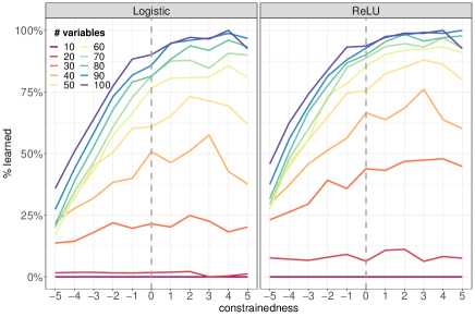
(a) Individuals

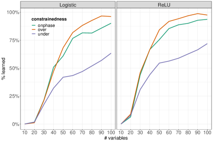
(b) Grouped

Figure 1: Percent of (perfectly) learned formulas, i.e. with 100% accuracy, according to the number of variables and constrainedness. In LABEL:sub@fig:individuals, the constrainedness appears in the x axis: underconstrained from -5 to -1, on phase at the vertical line on 0 and overconstrained from 1 to 5. In LABEL:sub@fig:grouped, the number of variables is in the x axis and each line shows the average % of learned formulas for constrainedness grouped into under, on phase and overconstrained.

#variables	Phase $c/v$	Source
10	5.500	CA
20	4.550	CA
30	4.433	CA
40	4.375	CA
50	4.360	SML
60	4.317	CA
70	4.300	CA
80	4.287	CA
90	4.289	CA
100	4.310	SML

Table 3: Satisfiability phase transition on random 3-CNFs according to the number of variables. Source is the paper where $c/v$ was obtained: CA [11] or SML [47].

In this section we investigate how hardness in satisfiability relates to hardness in learnability on random 3-CNF formulas. Our formulas range from 10 to 100 variables in increments of 10. These are relatively small to what SOTA SAT solvers routinely solve. This is on purpose because very large formulas were easily learned (Section 4.1) and the set with the smallest 3-GCP formulas was the hardest among sets with varying number of variables (Section 4.2).

For each number of variables, we generate sets of formulas with 11 values of constrainedness: 1 set on phase, 5 underconstrained sets (with on-phase $c/v$ subtracted by $0.1,0.2,\ldots,0.5$), and 5 overconstrained sets (with on-phase $c/v$ added by $0.1,0.2,\ldots,0.5$). Each set contains 1000 formulas. We use CNFgen [30] to generate a total of $10\times 11\times 1000=$ 110,000 satisfiable boolean formulas in this study (satisfiability was verified with MiniSAT [53]).

We assess the learnability of each generated formula as follows: train a single-hidden-layer neural network on the dataset generated for the formula, varying the number of hidden-layer neurons from 1 to 256 in powers of 2, and check how many neurons are sufficient to “learn” the formula perfectly (with 100% accuracy on the 5-fold cross validation). If perfect accuracy is not achieved with 256 neurons, we say that the formula has not been (perfectly) learned.

We test neural networks with ReLU and logistic (sigmoid) activation functions. Figure 1 shows, for each activation function, the percent of perfectly-learned formulas according to the number of variables and constrainedness, which we depict as ranging from -5 denoting the least constrained, 0 being on phase transition (hardest solubility) and +5 denoting the most constrained.

Interestingly, the smaller the formulas, the harder it is to learn them. In fact, no 10-variable formula was perfectly learned at all, regardless of the constrainedness (Fig. 1a). The ReLU neural network learned more formulas overall compared to logistic, specially with fewer variables. This is aligned with experimental [39, 12] and theoretical [15] evidence favouring ReLU over other activation functions in deep learning.

Figure 1 also shows that as constrainedness increases up to a point, more formulas are learned. Beyond such point, learnability slightly drops for all formulas, except those with 40 variables, where the drop is sharp on both activations. The point of highest learnability never coincides with the point of hardest solubility (the phase transition point, highlighted by the vertical dashed line in Fig. 1a).

Figure 1b highlights the similarity on the behaviour of onphase and overconstrained formulas as the number of variables increase, in contrast with underconstrained formulas. Learnability of on phase and overconstrained formulas grows almost identically with less than 40 variables. Beyond this point, overconstrained formulas become easier to learn. Alongside the percentage of perfectly-learned formulas, we assess the network complexity by measuring the average number of neurons needed to learn the formulas. Figure 2 shows the average number of neurons for each number of variables and constrainedness.

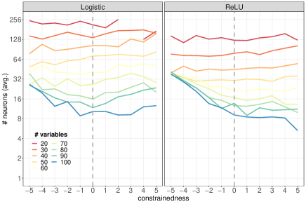
(a) Individuals

(b) Grouped

Figure 2: Average number of neurons required to learn the formulas of each number of variables and constrainedness. No line with 10 variables appears because no such formulas were perfectly learned at all (see Fig. 1). In LABEL:sub@fig:avg-individuals, the constrainedness appears in the x axis: underconstrained from -5 to -1, on phase at the vertical line on 0 and overconstrained from 1 to 5. The discontinuity with 20 variables and logistic activation happened because no formula with constrainedness=3 was learned. In LABEL:sub@fig:grouped, the number of variables is in the x axis and each line shows the average number of neurons for constrainedness grouped into under, on phase and overconstrained.

Smaller formulas require more neurons to be learned. With logistic activation, the required number of neurons varies only slightly with few variables, regardless of the constrainedness. From 80 or more variables, the required number of neurons seem to relate with the difficulty in satisfiability: easy-to-solve formulas (either low or high constrainedness) require more neurons to learn, whereas hard-to-satisfy formulas (on phase transition) require less neurons. The stability of the number of neurons required to learn smaller formulas regardless of their constrainedness also occurs with ReLU. Moreover, the number of neurons required to learn formulas with 30 to 100 variables is very similar for the smallest constrainedness. Differently from logistic activation, where the average number of neurons is the highest for under- and overconstraned formulas, with ReLU activation, the overall trend is a monotonic decrease on the number of neurons as the constrainedness increases.

Figure 2b further shows that networks with logistic activation behave similarly when formulas are grouped by their constrainedness, i.e., requiring less neurons for larger formulas. On ReLU networks, however, the required number of neurons for underconstrained formulas decreases much slower with more than 50 variables compared to on phase and overconstrained. Fig. 2b also highlights that ReLU neural networks are more efficient in the sense of requiring less neurons to learn on-phase or overconstrained formulas. On larger underconstrained formulas, logistic neural networks are more efficient. We remark that these results apply to the formulas that have been (perfecly-)learned, as ReLU neural nets were able to effectively learn more formulas (Fig. 1), regardless of constrainedness.

4.4 Symbolic vs. Neural Network Learning

Statistics / Clauses	350	400	420	431	450
VA Accuracy	0.62 (0.04)	0.81 (0.12)	0.91 (0.10)	0.91 (0.09)	0.95 (0.07)
NN Accuracy	0.99 (0.00)	0.99 (0.00)	1.00	1.00 (0.00)	1.00 (0.00)
VA F1-Score	0.37 (0.12)	0.74 (0.20)	0.88 (0.15)	0.89 (0.13)	0.92 (0.10)
NN F1-Score	0.99 (0.00)	0.99 (0.00)	1.00 (0.00)	1.00 (0.00)	1.00 (0.00)
#pos training	372.1 (33.83)	348.6 (73.22)	322.4 (83.10)	322.0 (80.84)	276.2 (119.34)
#neg training	375.0 (0.00)	375.0 (0.10)	375.0 (0.17)	375.0 (0.10)	375.0 (0.10)
#pos test	124.7 (11.32)	116.7 (24.50)	108.0 (27.81)	107.8 (27.50)	92.5 (39.90)
#neg test	125.0 (0.00)	125.0 (0.10)	125.0 (0.17)	125.0 (0.10)	125.0 (0.10)
Count	2087158074	11682341	1964898	413014	47582
$c/v$	3.50	4.00	4.20	4.31	4.50
$p/n$ training	0.992	0.930	0.860	0.859	0.737
$p/n$ test	0.997	0.934	0.864	0.863	0.740

Table 4: Results of Valiant’s algoritm (VA) vs the deep NN. Values present the average with std. deviation in parenthesis. #pos and #neg are the number of positive and negative assignments. Count is the average number of solutions of the set. $c/v$ is the clause-to-variable ratio (all formulas have 100 variables). $p/n$ is the positive-to-negative ratio of the assignments.

This section illustrates the performance of symbolic and deep neural network approaches. We generated sets of synthetic 3-CNF SAT formulas with 100 variables and 350, 400, 420, 431, and 450 clauses, respectively. Assignments of formulas were randomly divided into training (80%) and testing (20%) and used as an input dataset. For evaluation, we use the accuracy and F1-Score metrics and report positives, negatives, and number of solutions using Ganak [49]. Formulas with fewer clauses present an exponentially larger number of solutions than those with more clauses (Table 4). In this scenario, the search (learning) space is extensive, and the number of assignments is approximately equivalent for positives and negatives. The symbolic method (VA) learning procedure shows difficulties in generalizing from training to the test set (memorization of formulas). The accuracy of VA increases as the number of clauses increases; the mean value ranges from 62% (350 clauses) to 95% (450 clauses). This result is interesting because VA always reaches 100% training accuracy, but instead of learning, it memorizes the training data and generalizes poorly. Additionally, the ratio of positives and negatives solutions could direct this result because VA learns based on positives solutions in the learning space. Conversely, the neural network approach generalizes their learning better, independently of the number of clauses and the ratio of positives and negatives assignments.

5 Conclusions

The recent success of deep learning techniques over various domains and the positive theoretical results on the learnability of boolean formulas prompts the question of how effective DL approaches are in learning boolean formulas, which encode relevant problems in a variety of relevant domains, including symbolic reasoning and combinatorial optimization. We have tackled this subject by assessing the learning capabilities of multi-layer perceptrons (MLPs) – the basic components of deep learning systems – over boolean formulas encoding large model sampling benchmarks, combinatorial optimization problems, and random 3-CNFs with various constrainedness (clause-to-variable ratios). Our methodology consists of generating positive (satisfying) and negative (falsifying) examples for each formula, and verifying the cross-validation (CV) accuracy of a MLP as a means to assess its capability to learn the formula.

MLPs were very good approximators of all studied formulas, with no cross-validation accuracy below 99%. We thus use the more challenging measure of how many formulas were perfectly learned, i.e. with 100% CV accuracy, as a proxy for learnability. Our extensive experiments have four main findings:(i) neural learning generalizes better than pure rule-based systems (Section 4.1) and pure symbolic approach (Sect. 4.4); (ii) relatively small and shallow neural networks can learn several families of boolean functions that encode combinatorial optimization problems (Sect. 4.2); (iii) smaller formulas seem harder to learn, possibly due to the fewer positive (satisfying) examples available; and (iv) interestingly, underconstrained 3-CNF formulas are more challenging to learn than overconstrained ones (Sect. 4.3). Our results can foster more empirical or new theoretical studies on the learning capabilities of deep learning models. For example, it would be interesting to further investigate whether the harder learnability of small formulas is associated with the better “coverage” of their datasets (since their size is fixed in our experiments, they are more sparse for large formulas), or some property of their factor graphs (as in [65], where edges connect variables to clauses). Another line of future work could focus on gaining insights of what the neural networks have learned. This can be done via explainability methods (e.g. SHAP [33]) or the deduction procedure mentioned by [59], where we would extract the formula learned by the MLP (using knowledge extraction methods [57]) and check to which extent it matches the original one.

References

- [1] Martin Anthony. Neural networks and boolean functions. In Y. Crama and P.L. Hammer, editors, Boolean Models and Methods in Mathematics, Computer Science, and Engineering, pages 554–576. Cambridge U. Press, 2010.
- [2] Sanjeev Arora and Boaz Barak. Computational Complexity: A Modern Approach. Cambridge University Press, 2009.
- [3] Gilles Audemard and Laurent Simon. On the Glucose SAT solver. Intl. J. on Artif. Intel. Tools, 27(01):1840001, 2018.
- [4] Clark Barrett, Aaron Stump, Cesare Tinelli, et al. The SMT-lib standard: Version 2.0. In Proc. 8th Intl. Workshop on Satisfiability modulo theories, 2010.
- [5] Azam Beg, PW Chandana Prasad, and Ajmal Beg. Applicability of feed-forward and recurrent neural networks to boolean function complexity modeling. Expert Sys. With Appl., 34(4):2436–2443, 2008.
- [6] E. K. Blum. Approximation of boolean functions by sigmoidal networks: Part i: Xor and other two-variable functions. Neural Computation, 1(4):532–540, 1989.
- [7] Béla Bollobás and Paul Erdos. Cliques in random graphs. In Mathematical Proceedings of the Cambridge Philosophical Society, volume 80, pages 419–427. Cambridge Univ Press, 1976.
- [8] Supratik Chakraborty, Daniel Fremont, Kuldeep Meel, Sanjit Seshia, and Moshe Vardi. On parallel scalable uniform sat witness generation. In TACAS, pages 304–319, 2015.
- [9] Peter Cheeseman, Bob Kanefsky, and William Taylor. Where the really hard problems are. In IJCAI, pages 331–337, 1991.
- [10] Gabriele Ciravegna, Pietro Barbiero, Francesco Giannini, Marco Gori, Pietro Lió, Marco Maggini, and Stefano Melacci. Logic Explained Networks, 2021.
- [11] James Crawford and Larry Auton. Experimental results on the crossover point in random 3-sat. Art. Intel., 81:31–57, 1996.
- [12] G. E. Dahl, T. N. Sainath, and G. E. Hinton. Improving deep neural networks for lvcsr using rectified linear units and dropout. In ICASSP, pages 8609–8613, 2013.
- [13] Amit Daniely. SGD Learns the Conjugate Kernel Class of the Network. In NIPS, volume 30. Curran Associates, Inc., 2017.
- [14] P. Erdös and A. Rényi. On random graphs i. Publicationes Mathematicae, 6(1-2):290–297, 1959.
- [15] Jonathan Fiat, Eran Malach, and Shai Shalev-Shwartz. Decoupling gating from linearity. CoRR, abs/1906.05032, 2019.
- [16] Leonardo Franco. Generalization ability of boolean functions implemented in feedforward neural networks. Neurocomputing, 70(1):351 – 361, 2006.
- [17] Leonardo Franco and Martin Anthony. On a generalization complexity measure for boolean functions. In IEEE IJCNN, volume 2, pages 973–978. IEEE, 2004.
- [18] Leonardo Franco and Martin Anthony. The influence of oppositely classified examples on the generalization complexity of boolean functions. IEEE Transactions on Neural Networks, 17(3):578–590, 2006.
- [19] A. Galassi, K. Kersting, M. Lippi, X. Shao, and P. Torroni. Neural-symbolic argumentation mining: an argument in favour of deep learning and reasoning. Frontiers in Big Data, 2:52, 2020.
- [20] A. Garcez, M. Gori, L. Lamb, L. Serafini, M. Spranger, and S. Tran. Neural-symbolic computing: An effective methodology for principled integration of machine learning and reasoning. FLAP, 6(4):611–632, 2019.
- [21] A. d’Avila Garcez, L.C. Lamb, and D.M. Gabbay. Neural-Symbolic Cognitive Reasoning. Springer, 2009.
- [22] Pascale Gourdeau, Varun Kanade, Marta Kwiatkowska, and James Worrell. On the hardness of robust classification. In NeurIPS, pages 7446–7455, 2019.
- [23] Tad Hogg. Refining the phase transition in combinatorial search. Artificial Intelligence, 81(1-2):127–154, 1996.
- [24] D. Kahneman, G. Hinton, Y. Bengio, Y. LeCun, and F. Rossi. AAAI-20 fireside chat with Daniel Kahneman. https://vimeo.com/390814190?ref=tw-share, 2020. Accessed: 2020-08-30.
- [25] Michael Kearns, Yishay Mansour, Dana Ron, Ronitt Rubinfeld, Robert E Schapire, and Linda Sellie. On the learnability of discrete distributions. In ACM STOC, pages 273–282, 1994.
- [26] Michael J. Kearns, Ming Li, and Leslie G. Valiant. Learning boolean formulas. J. ACM, 41(6):1298–1328, 1994.
- [27] Michael J Kearns and Umesh Vazirani. An introduction to computational learning theory. MIT press, 1994.
- [28] Diederik P Kingma and Jimmy Ba. Adam: A method for stochastic optimization. arXiv preprint arXiv:1412.6980, 2014.
- [29] Donald E. Knuth. The Art of Computer Programming, Vol. 4, Fascicle 0: Introduction to Combinatorial Algorithms and Boolean Functions. Addison-Wesley Professional, 1 edition, 2008.
- [30] Massimo Lauria, Jan Elffers, Jakob Nordström, and Marc Vinyals. CNFgen: Combinatorial benchmarks for SAT solvers, 2019.
- [31] Y. LeCun, Y. Bengio, and G. Hinton. Deep learning. Nature, 521(7553):436–444, 2015.
- [32] Yichao Liang, Joshua B Tenenbaum, Tuan Anh Le, and N Siddharth. Drawing out of distribution with neuro-symbolic generative models. arXiv preprint arXiv:2206.01829, 2022.
- [33] S. Lundberg and Su-In Lee. A Unified Approach to Interpreting Model Predictions. In NIPS, pages 4765–4774, 2017.
- [34] J. Mao, C. Gan., P. Kohli, J. Tenenbaum, and J. Wu. The Neuro-Symbolic Concept Learner: Interpreting scenes, words, and sentences from natural supervision. In ICLR, 2019.
- [35] Jiayuan Mao, Zhezheng Luo, Chuang Gan, Joshua B. Tenenbaum, Jiajun Wu, Leslie Pack Kaelbling, and Tomer D. Ullman. Temporal and object quantification networks. In Zhi-Hua Zhou, editor, Proceedings of the Thirtieth International Joint Conference on Artificial Intelligence, IJCAI-21, pages 2804–2811. International Joint Conferences on Artificial Intelligence Organization, 8 2021. Main Track.
- [36] G. Marcus. The next decade in AI: Four steps towards robust artificial intelligence. CoRR, abs/1801.00631, 2020.
- [37] Kuldeep S. Meel. Sampling Techniques for Boolean Satisfiability, 2014.
- [38] Julian F Miller. An empirical study of the efficiency of learning boolean functions using a Cartesian Genetic Programming approach. In GECCO, pages 1135–1142, 1999.
- [39] Vinod Nair and Geoffrey Hinton. Rectified Linear Units Improve Restricted Boltzmann Machines. In ICML, pages 807–814, 2010.
- [40] Xingyuan Pan and Vivek Srikumar. Expressiveness of rectifier networks. In ICML, page 2427–2435. JMLR.org, 2016.
- [41] F. Pedregosa, G. Varoquaux, A. Gramfort, V. Michel, B. Thirion, O. Grisel, M. Blondel, P. Prettenhofer, R. Weiss, V. Dubourg, J. Vanderplas, A. Passos, D. Cournapeau, M. Brucher, M. Perrot, and E. Duchesnay. Scikit-learn: Machine learning in Python. JMLR, 12:2825–2830, 2011.
- [42] PW Chandana Prasad and Azam Beg. Investigating data preprocessing methods for circuit complexity models. Expert Systems with Applications, 36(1):519–526, 2009.
- [43] L. De Raedt, S. Dumancic, R. Manhaeve, and G. Marra. From statistical relational to neuro-symbolic artificial intelligence. CoRR, abs/2003.08316, 2020.
- [44] S. Raghavan. 2020 AI predictions from IBM research. https://www.ibm.com/blogs/research/2019/12/2020-ai-predictions/, 2019. Accessed: 2020-08-20.
- [45] Ronald L Rivest. Cryptography and machine learning. In International Conference on the Theory and Application of Cryptology, pages 427–439. Springer, 1991.
- [46] Jürgen Schmidhuber. Deep learning in neural networks: An overview. Neural Networks, 61:85–117, 2015.
- [47] Bart Selman, David G Mitchell, and Hector J Levesque. Generating hard satisfiability problems. Artificial Intelligence, 81(1–2):17–29, 1996.
- [48] Prithviraj Sen, Breno W. S. R. de Carvalho, Ryan Riegel, and Alexander G. Gray. Neuro-symbolic inductive logic programming with logical neural networks. In Thirty-Sixth AAAI Conference on Artificial Intelligence, AAAI 2022, Thirty-Fourth Conference on Innovative Applications of Artificial Intelligence, IAAI 2022, The Twelveth Symposium on Educational Advances in Artificial Intelligence, EAAI 2022 Virtual Event, February 22 - March 1, 2022, pages 8212–8219. AAAI Press, 2022.
- [49] Shubham Sharma, Subhajit Roy, Mate Soos, and Kuldeep S Meel. Ganak: A scalable probabilistic exact model counter. In IJCAI, volume 19, pages 1169–1176, 2019.
- [50] Yoan Shin and Joydeep Ghosh. Realization of boolean functions using binary pi-sigma networks. In Proc. Conf. on Artificial Neural Networks in Engineering, pages 205–210, 1991.
- [51] Tom Silver, Ashay Athalye, Joshua B Tenenbaum, Tomas Lozano-Perez, and Leslie Pack Kaelbling. Learning neuro-symbolic skills for bilevel planning. arXiv preprint arXiv:2206.10680, 2022.
- [52] Mate Soos, Stephan Gocht, and Kuldeep S Meel. Tinted, detached, and lazy CNF-XOR solving and its applications to counting and sampling. In CAV, pages 463–484. Springer, 2020.
- [53] Niklas Sorensson and Niklas Een. MiniSat: A SAT Solver with Conflict-Clause Minimization. In SAT’03, pages 1–2, 2003.
- [54] Bernd Steinbach and Roman Kohut. Neural networks–a model of boolean functions. In 5th Int. Workshop on Boolean Problems, pages 223–240, 2002.
- [55] José L Subirats, José M Jerez, and Leonardo Franco. A new decomposition algorithm for threshold synthesis and generalization of boolean functions. IEEE T. Circuits and Systems I, 55(10):3188–3196, 2008.
- [56] José Luis Subirats, Iván Gómez, José M Jerez, and Leonardo Franco. Optimal synthesis of boolean functions by threshold functions. In ICANN, pages 983–992. Springer, 2006.
- [57] S. Tran and A. Garcez. Deep logic networks: Inserting and extracting knowledge from deep belief networks. IEEE T. Neur. Net. Learning Syst., 29:246–258, 2018.
- [58] Hiroshi Tsukimoto. Extracting propositions from trained neural networks. In IJCAI, pages 1098–1105, 1997.
- [59] L. G. Valiant. A theory of the learnable. Commun. ACM, 27(11):1134–1142, November 1984.
- [60] Leslie G. Valiant. Probably Approximately Correct: Nature’s Algorithms for Learning and Prospering in a Complex World. Basic Books, New York, 2013.
- [61] L.G. Valiant. Three problems in computer science. J. ACM, 50(1):96–99, 2003.
- [62] S. van Steenkiste, M. Chang, K. Greff, and J. Schmidhuber. Relational neural expectation maximization: Unsupervised discovery of objects and their interactions. ICLR, 2018.
- [63] V. N. Vapnik and A. Ya. Chervonenkis. On the Uniform Convergence of Relative Frequencies of Events to Their Probabilities. Theory of Probabilities and its Applications, 16(2):264–280, 1971.
- [64] Xuan Xie, Kristian Kersting, and Daniel Neider. Neuro-symbolic verification of deep neural networks. In Luc De Raedt, editor, Proceedings of the Thirty-First International Joint Conference on Artificial Intelligence, IJCAI 2022, Vienna, Austria, 23-29 July 2022, pages 3622–3628. ijcai.org, 2022.
- [65] Emre Yolcu and Barnabás Póczos. Learning local search heuristics for boolean satisfiability. In NeurIPS, pages 7992–8003, 2019.
- [66] C. Zhang, J. Yang, and W. Wu. Binary higher order neural networks for realizing boolean functions. IEEE Transactions on Neural Networks, 22(5):701–713, 2011.
- [67] Zhaozhi Zhang, Xiaomin Ma, and Yixian Yang. Bounds on the number of hidden neurons in three-layer binary neural networks. Neural networks, 16(7):995–1002, 2003.