Attention Cube Network for Image Restoration

Abstract.

Recently, deep convolutional neural network (CNN) have been widely used in image restoration and obtained great success. However, most of existing methods are limited to local receptive field and equal treatment of different types of information. Besides, existing methods always use a multi-supervised method to aggregate different feature maps, which can not effectively aggregate hierarchical feature information. To address these issues, we propose an attention cube network (A-CubeNet) for image restoration for more powerful feature expression and feature correlation learning. Specifically, we design a novel attention mechanism from three dimensions, namely spatial dimension, channel-wise dimension and hierarchical dimension. The adaptive spatial attention branch (ASAB) and the adaptive channel attention branch (ACAB) constitute the adaptive dual attention module (ADAM), which can capture the long-range spatial and channel-wise contextual information to expand the receptive field and distinguish different types of information for more effective feature representations. Furthermore, the adaptive hierarchical attention module (AHAM) can capture the long-range hierarchical contextual information to flexibly aggregate different feature maps by weights depending on the global context. The ADAM and AHAM cooperate to form an ”attention in attention” structure, which means AHAM’s inputs are enhanced by ASAB and ACAB. Experiments demonstrate the superiority of our method over state-of-the-art image restoration methods in both quantitative comparison and visual analysis.

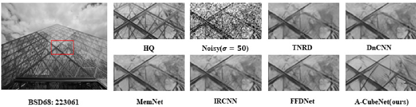
Figure 1. Gray image denoising results with noise level 50 on “BSD: 223061” from BSD68. Our method obtains better visual quality and recovers more textural details compared with other state-of-the-art methods.

Gray image denoising results with noise level 50 on “BSD: 223061” from BSD68. Our method obtains better visual quality and recovers more textural details compared with other state-of-the-art methods.

1. Introduction

Image restoration is a classic computer vision task that aims to recover high-quality images from low-quality images corrupted by various kinds of degradations. Due to the irreversible nature of the image degradation process, it is an ill-posed problem. It can be categorized into different tasks such as image super-resolution, image denoising, JPEG image deblocking, etc.

Recently, methods based on deep convolutional neural network (CNN) have been widely used in image restoration due to their strong nonlinear representational power. (Dong et al., 2015b; Kim et al., 2016a, b; Haris et al., 2018; Zhang et al., 2018b, a; Dai et al., 2019; Hui et al., 2019) focused on designing a deeper, wider or lighter network structure, aiming at improving the performance of image super-resolution. Dong et al.(Dong et al., 2015a) proposed ARCNN with several stacked convolutional layers for JPEG image deblocking. By taking a tunable noise level map as input, FFDNet can deal with noise on different levels (Zhang et al., 2018c). Guo et al.(Guo et al., 2019) proposed CBDNet for blind denoising of real images. However, these methods are for specific image restoration tasks. Different from them, (Liu et al., 2018a, b; Zhang et al., 2017a, b, 2019) developed a couple of valuable methods that can be generalized to different image restoration tasks.

Although above CNN-based image restoration methods have achieved gratifying results, they still have some problems: (1) The receptive fields of these methods are relatively small. Most of these methods extract features in a local way through convolution operations, which cannot capture the long-range dependencies between pixels in the whole image. A larger receptive field can make better use of training images and more contextual information, which is very helpful for image restoration, especially when the images suffer from heavy corruptions. (2) Most of these methods treat all types of information (e.g., low and high frequency information) equally, which may result in over-smoothed reconstructed images and fail to recover some textural details. In other words, the power of discrimination of these methods is limited. (3) In response to problem one and two, although there have been recent methods that use attention mechanism (e.g., SENet (Hu et al., 2018) and non-local neural network (Wang et al., 2018)) for image super-resolution, most methods directly introduce the attention mechanism in high-level computer vision tasks and ignore the difference between high-level and low-level computer vision tasks (Zhang et al., 2018a; Dai et al., 2019). (4) Most of these methods only use the feature map outputted from the last layer for image restoration. In fact, in deep convolutional neural networks, feature map information at different levels can complement each other. If only the feature map outputted from the last layer is used for image restoration, part of the information is bound to be lost. Although there are some methods that take this problem into account, they just cascade them together (Zhang et al., 2018b) or use a multi-supervised method (Kim et al., 2016b; Tai et al., 2017b), and the feature map information of each level is not fully and effectively used.

In order to solve above problems, this paper proposes an attention cube network (A-CubeNet) for image restoration based on adaptive dual attention module (ADAM) and adaptive hierarchical attention module (AHAM). Specifically, this paper proposes an adaptive dual attention module for above mentioned problem one, two, and three. This module can capture the long-range dependencies between pixels and channels to expand the receptive field and distinguish different types of information for more effective feature representations, which is very helpful for the restoration of textural details. In addition, inspired by the non-local neural network, this paper designs an adaptive hierarchical attention module for above mentioned problem four. This module first performs squeeze operations on the spatial and channel-wise dimensions of each feature map for global context modeling. Then this module captures the long-range dependencies between different feature maps. Finally, this module fuses each feature map based on the long-range dependencies between different feature maps. Full experiments show that compared with other state-of-the-art methods, our A-CubeNet achieves the best results in all tasks.

In summary, the main contributions of this paper are listed as follows:

$\bullet$ We propose an adaptive dual attention module (ADAM), including an adaptive spatial attention branch (ASAB) and an adaptive channel attention branch (ACAB). ADAM can capture the long-range spatial and channel-wise contextual information to expand the receptive field and distinguish different types of information for more effective feature representations. Therefore our A-CubeNet can obtain high-quality image restoration results, as shown in Figure 1.

$\bullet$ Inspired by the non-local neural network, we design an adaptive hierarchical attention module (AHAM), which flexibly aggregates all output feature maps together by the hierarchical attention weights depending on global context. To the best of our knowledge, this is the first time to consider aggregating output feature maps in a hierarchical attention method with global context.

$\bullet$ Through sufficient experiments, we prove that our A-CubeNet is powerful for various image restoration tasks. Compared with other state-of-the-art methods for image denoising, JPEG image deblocking and image super-resolution, our A-CubeNet obtains superior results in both quantitative metrics and visual quality.

2. related work

2.1. Image Restoration

CNN-based image restoration methods cast image restoration as an image-to-image regression problem, and learn an end-to-end mapping from low-quality (LQ) to high-quality (HQ) directly. Dong et al. (Dong et al., 2014, 2015a) proposed SRCNN for image super resolution and ARCNN for JPEG image deblocking. Both of them achieved superior performance against previous methods that are not based on CNN. Then (Kim et al., 2016a, b; Haris et al., 2018; Zhang et al., 2018b, a; Dai et al., 2019; Hu et al., 2019) focused on designing a deeper and wider network structure or considering feature correlations to improve the performance of image super-resolution. Zhang et al. (Zhang et al., 2017a) proposed DnCNN for image denoising and JPEG image deblocking by introducing residual learning to train deeper network. (Zhang et al., 2017b) introduced the denoiser prior for fast image restoration. Tai et al. (Tai et al., 2017b) lately designed a persistent memory network for image restoration and achieved promising results. However, most methods neglect to consider feature correlations in spatial or channel-wise dimensions and can not make full use of hierarchical feature maps.

2.2. Attention Mechanism

Attention mechanism is inspired by the cognitive process of human (Mnih et al., 2014). Human always focuses on more important information. Attention mechanism has been widely used in various computer vision tasks, such as image and video classification tasks (Hu et al., 2018; Wang et al., 2018). Wang et al. (Wang et al., 2018) proposed non-local neural network by incorporating non-local operations for spatial attention in video classification. (Hu et al., 2018) modelled channel-wise relationships to obtain significant performance gain for image classification. Woo et al. (Woo et al., 2018) developed CBAM to model both channel-wise and spatial relationships. In all, these works mainly aimed to concentrate on more useful information in features.

Recently, SENet was introduced to improve SR performance (Zhang et al., 2018a). (Hu et al., 2019; Kim et al., 2018; Dai et al., 2019) focused on introducing both channel attention and spatial attention to image super-resolution. Dai et al. (Dai et al., 2019) designed a second-order attention mechanism based on SENet and introduced non-local neural network to further improve SR performance. Following the importance of self-similarity prior, (Zhang et al., 2019) adapted non-local operations into their network. However, most methods directly introduce the attention mechanism in high-level computer vision tasks and ignore the difference between high-level and low-level computer vision tasks. For example, non-local neural network is computationally intensive and is actually not suitable for image restoration.

3. method

3.1. Framework

As shown in Figure 2, the proposed A-CubeNet mainly consists of three modules: the shallow feature extraction module, the deep feature extraction module stacked with G residual dual attention groups (RDAGs) and one adaptive hierarchical attention module (AHAM), and the construction module. Given $I_{LQ}$ and $I_{HQ}$ as the low-quality (e.g., noisy, low resolution, or compressed images) and high-quality images. We apply only one convolutional layer to extract the shallow feature $F_{0}$ from the low-quality input:

(1) $$F_{0}=H_{SF}\left(I_{LQ}\right)\text{, }$$

where $H_{SF}(\cdot)$ represents the shallow feature extraction module. Then the extracted shallow feature $F_{0}$ is used for RDAGs and AHAM based deep feature extraction, which thus produces the deep feature as:

(2) $$F_{DF}=H_{DF}\left(F_{0}\right)=F_{0}+W_{LSC}H_{AHAM}\left(F_{1},\cdots,F_{g},\cdots,F_{G}\right)\text{, }$$

where $H_{DF}(\cdot)$, $W_{LSC}$ and $H_{AHAM}(\cdot)$ represent the deep feature extraction module, the convolutional layer at the end of the deep feature extraction module and the adaptive hierarchical attention module (AHAM), respectively. To address the image super-resolution task, we add an extra upscale layer before the last convolutional layer. Specifically, we utilize sub-pixel convolutional operation (convolution + pixel shuffle) (Shi et al., 2016) to upscale feature maps:

(3) $$F_{UP}=H_{UP}\left(F_{DF}\right)\text{, }$$

where $H_{UP}(\cdot)$ represents the upscale module. Then we use a convolutional layer to get the reconstructed image:

(4) $$I_{REC}=H_{REC}\left(F_{DF}\right)\text{ or }I_{REC}=H_{REC}\left(F_{UP}\right)\text{, }$$

where $H_{REC}(\cdot)$ represents the reconstruction module. The overall reconstruction process can be expressed as:

(5) $$I_{REC}=H_{A-CubeNet}\left(I_{LQ}\right)\text{, }$$

where $H_{A-CubeNet}(\cdot)$ represents the function of our A-CubeNet.

Then A-CubeNet is optimized with a certain loss function. Some loss functions have been widely adopted, such as L2 (Zhang et al., 2017a, b; Tai et al., 2017b; Dong et al., 2015a), L1 (Lim et al., 2017; Zhang et al., 2018b; Dai et al., 2019), perceptual and adversarial losses (Ledig et al., 2017). To verify the effectiveness of our A-CubeNet, we adopt the same loss functions as previous works (e.g., L1 loss function for image super-resolution, L2 loss function for image denoising and JPEG image deblocking). Given a training set $\left\{I_{LQ}^{i},I_{HQ}^{i}\right\}_{i=1}^{N}$ with N LQ images and their HQ counterparts. The goal of training A-CubeNet is to optimize the loss function:

(6) $$L_{1}(\theta)=\frac{1}{N}\sum_{i=1}^{N}\left\|H_{A-CubeNet}\left(I_{LQ}^{i}\right)-I_{HQ}^{i}\right\|_{1}\text{, }$$

$$L_{2}(\theta)=\frac{1}{N}\sum_{i=1}^{N}\left\|H_{A-CubeNet}\left(I_{LQ}^{i}\right)-I_{HQ}^{i}\right\|_{2}\text{, }$$

where $\theta$ indicates the updateable parameters of our A-CubeNet.

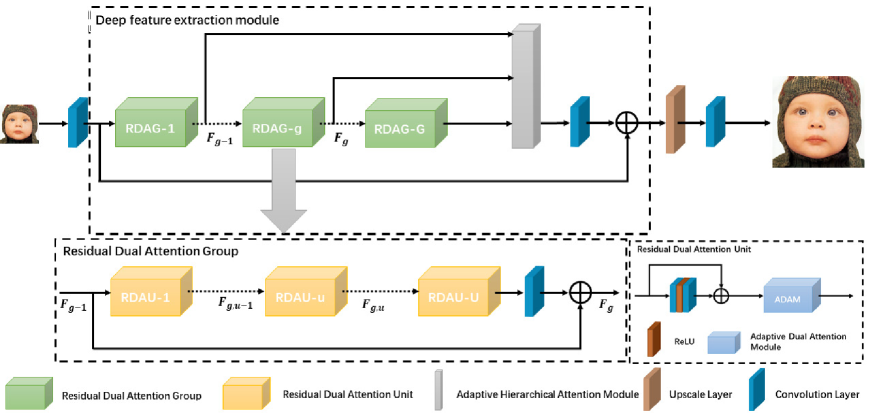
Figure 2. Framework of the proposed attention cube network (A-CubeNet)

Framework of the proposed attention cube network (A-CubeNet)

3.2. Residual Dual Attention Group (RDAG)

As shown in Figure 2, the deep feature extraction module stacked with several RDAGs, while an RDAG consists of two parts: U stacked RDAUs and one convolutional layer. The g-th RDAG can be expressed as:

(7) $$F_{g}=F_{g-1}+W_{SSC}H_{g,u}\left(H_{g,u-1}\left(\cdots H_{g,1}\left(F_{g-1}\right)\cdots\right)\right)\text{, }$$

where $F_{g-1}$ and $F_{g}$ represent the input and output of the g-th RDAG. $W_{SSC}$ and $H_{g,u}(\cdot)$ represent the convolutional layer at the end of the g-th RDAG and the u-th RDAU of the g-th RDAG, respectively. Each RDAU consists of one residual block and one adaptive dual attention module (ADAM). Then we give more details to ADAM and AHAM.

3.3. Adaptive Dual Attention Module (ADAM)

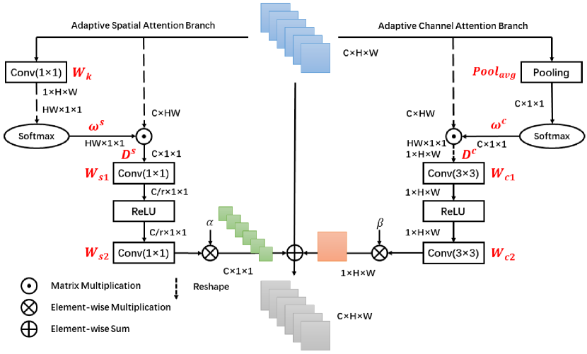
Figure 3. Adaptive dual attention module (ADAM)

Adaptive dual attention module

As shown in Figure 3, our adaptive dual attention module (ADAM) consists of two branches: adaptive spatial attention branch (ASAB) and adaptive channel attention branch (ACAB). These two branches cooperate to draw global features rather than local features and endow the network the ability to treat different types of information differently. Thus our A-CubeNet obtains better feature representations for high-quality image restoration. Take the adaptive spatial attention branch in Figure 3 as an example. First, we apply a convolutional layer to squeeze channel-wise features and apply softmax function to obtain the attention weights. Second, we perform a matrix multiplication between the attention weights and the original features to obtain long-range spatial contextual information. Third, we perform feature transform and feature fusion with adaptive weight. Similarly, we obtain channel-wise long-range contextual information by the adaptive channel attention branch. In general, each branch has three steps: (1) Squeeze features; (2) Extract long-range contextual information; (3) Perform feature fusion with adaptive weight. Our ADAM can be formulated as:

(8) $$Out_{ADAM}=X+Out_{ASAB}+Out_{ACAB}\text{, }$$

where X , $Out_{ASAB}$, $Out_{ACAB}$ and $Out_{ADAM}$ represent the input feature map, the output of ASAB, the output of ACAB and the output feature map of ADAM, respectively.

3.3.1. Adaptive spatial attention branch (ASAB)

As shown in Figure 3, given an input feature map $X=\left\{X_{i}\right\}_{i=1}^{N}$, $X\in\mathbb{R}^{C\times H\times W}$, where $N=H\times W$ is the number of pixels. First, we apply a convolutional layer $W_{k}$ to squeeze channel-wise features: $A^{s}=W_{k}X$, $A^{s}\in\mathbb{R}^{1\times H\times W}$. Then we reshape it to $\mathbb{R}^{HW\times 1\times 1}$ and apply a softmax fuction to obtain the spatial attention weights $\omega^{s}\in\mathbb{R}^{HW\times 1\times 1}$:

(9) $$\omega^{s}_{j}=\frac{\exp\left(A^{s}_{j}\right)}{\sum_{m=1}^{N}\exp\left(A^{s}_{m}\right)}\text{, }$$

Then we reshape $X\in\mathbb{R}^{C\times H\times W}$ to obtain $B^{s}\in\mathbb{R}^{C\times HW}$. After that we perform long-range spatial contextual information modeling, which groups the features of all pixels together with the spatial attention weights to obtain the long-range spatial contextual features. Specifically, we perform a matrix multiplication between $B^{s}$ and the spatial attention weights $\omega^{s}$:

(10) $$D^{s}=\sum_{j=1}^{N}\omega^{s}_{j}B^{s}_{j}\text{, }$$

where $D^{s}\in\mathbb{R}^{C\times 1\times 1}$ represents spatial long-range contextual features. Then we feed it into a bottleneck network (e.g., one $1\times 1$ convolutional layer $W_{s1}$, one ReLU activation layer and one $1\times 1$ convolutional layer $W_{s2}$) to perform feature transform. Finally, we multiply it by an adaptive learning weight $\alpha$:

(11) $$Out_{ASAB} =\alpha W_{s2}\operatorname{ReLU}\left(W_{s1}\sum_{j=1}^{N}\omega^{s}_{j}B^{s}_{j}\right)$$

$$=\alpha W_{s2}\operatorname{ReLU}\left(W_{s1}\sum_{j=1}^{N}\frac{\exp\left(W_{k}X_{j}\right)}{\sum_{m=1}^{N}\exp\left(W_{k}X_{m}\right)}X_{j}\right)\text{. }$$

where $Out_{ASAB}\in\mathbb{R}^{C\times 1\times 1}$ represents the output of ASAB.

We emphasize three points: (1) $\alpha$ is initialized as 0 and gradually learns to assign larger weight. This adaptive learning weight helps our A-CubeNet fuse long-range spatial contextual features effectively. (2) We use a bottleneck network with the bottleneck ratio r instead of only one $1\times 1$ convolutional layer because: (a) Compared with using only one $1\times 1$ convolutional layer, the number of parameters reduces from $C^{2}$ to $2C^{2}/r$. (b) Just like SENet (Hu et al., 2018), it can better fit the complex correlation between channels with more nonlinearity. However, noted that this correlation between channels is directed at long-range spatial contextual features instead of the input feature map. So it can only be regarded as a supplement to the spatial attention mechanism. (3) The Equation 11 shows that $Out_{ASAB}$ is a weighted sum of the features across all pixels. Therefore, it has a global receptive field and selectively aggregates context according to the spatial attention weights.

3.3.2. Adaptive channel attention branch (ACAB)

As shown in Figure 3, given an input feature map $X=\left\{X_{i}\right\}_{i=1}^{C}$, $X\in\mathbb{R}^{C\times H\times W}$, where C is the number of channels. First, we apply an average pooling layer ${Pool}_{\text{avg }}$ to squeeze spatial features: $A^{c}={Pool}_{\text{avg }}X$, $A^{c}\in\mathbb{R}^{C\times 1\times 1}$. Then we apply a softmax fuction to obtain the channel-wise attention weights $\omega^{c}\in\mathbb{R}^{C\times 1\times 1}$:

(12) $$\omega^{c}_{j}=\frac{\exp\left(A^{c}_{j}\right)}{\sum_{m=1}^{C}\exp\left(A^{c}_{m}\right)}\text{, }$$

Then we reshape $X\in\mathbb{R}^{C\times H\times W}$ to obtain $B^{c}\in\mathbb{R}^{C\times HW}$. After that we perform long-range channel-wise contextual information modeling, which groups the features of all channels together with the channel-wise attention weights to obtain long-range channel-wise contextual features. Specifically, we perform a matrix multiplication between $B^{c}$ and the channel-wise attention weights $\omega^{c}$:

(13) $$D^{c}=\sum_{j=1}^{C}\omega^{c}_{j}B^{c}_{j}\text{, }$$

where $D^{c}\in\mathbb{R}^{C\times 1\times 1}$ represents channel-wise long-range contextual features. Then we feed it into a network (e.g., one $3\times 3$ convolutional layer $W_{c1}$, one ReLU activation layer and one $3\times 3$ convolutional layer $W_{c2}$) to perform feature transform. Finally, we multiply it by an adaptive learning weight $\beta$:

(14) $$Out_{ACAB} =\beta W_{c2}\operatorname{ReLU}\left(W_{c1}\sum_{j=1}^{C}\omega^{c}_{j}B^{c}_{j}\right)$$

$$=\beta W_{c2}\operatorname{ReLU}\left(W_{c1}\sum_{j=1}^{C}\frac{\exp\left(\operatorname{Pool}_{\text{avg }}X_{j}\right)}{\sum_{m=1}^{C}\exp\left(\operatorname{Pool}_{\text{avg }}X_{m}\right)}X_{j}\right)\text{. }$$

where $Out_{ACAB}\in\mathbb{R}^{1\times H\times W}$ represents the output of ACAB.

We emphasize three points: (1) $\beta$ is initialized as 0 and gradually learns to assign larger weight. This adaptive learning weight helps our AGAM fuse long-range channel-wise contextual features effectively. (2) We use a network instead of only one $3\times 3$ convolutional layer because it can better fit the complex spatial correlation with more nonlinearity, just like CSAR block (Hu et al., 2019). However, noted that this spatial correlation is directed at long-range channel-wise contextual features instead of the input feature map. So it can only be regarded as a supplement to the channel attention mechanism. (3) The Equation 14 shows that $Out_{ACAB}$ is a weighted sum of the features across all channels. It makes our A-CubeNet focus on more informative features and improve the power of discrimination.

3.4. Adaptive Hierarchical Attention Module (AHAM)

Figure 4. Adaptive hierarchical attention module (AHAM)

Adaptive hierarchical attention module

As shown in Figure 4, given a set of each residual dual attention group’s output feature map $F=\left\{F_{g}\right\}_{g=1}^{G}$, $F_{g}\in\mathbb{R}^{C\times H\times W}$, where G is the number of residual dual attention groups (RDAGs). First, we apply an average pooling layer ${Pool}_{\text{avg }}$ and a convolutional layer $W_{g}$ to squeeze global features of each feature map: $A^{h}_{g}=W_{g}{Pool}_{\text{avg }}F_{g}$, $A^{h}_{g}\in\mathbb{R}^{1\times 1\times 1}$. Then we cascade them to obtain $A^{h}\in\mathbb{R}^{1\times 1\times G\times 1}$. After that we apply a softmax function to obtain the hierarchical attention weights $\omega^{h}\in\mathbb{R}^{1\times 1\times G\times 1}$:

(15) $$\omega^{h}_{j}=\frac{\exp\left(A^{h}_{j}\right)}{\sum_{m=1}^{G}\exp\left(A^{h}_{m}\right)}\text{, }$$

Then we cascade each $F_{g}$ to obtain $B^{h}\in\mathbb{R}^{C\times H\times W\times G}$. After that we perform global contextual information modeling, which groups all RDAG’s output feature maps together with the self-adaptive weights to obtain global contextual features. Specifically, we perform a matrix multiplication between $B^{h}$ and the hierarchical attention weights $\omega^{h}$:

(16) $$D^{h}=\sum_{j=1}^{G}\omega^{h}_{j}B^{h}_{j}\text{, }$$

where $D^{h}\in\mathbb{R}^{C\times H\times W}$ represents global contextual features. Then, we multiply it by an adaptive learning weight $\gamma$. Finally, we perform an element-wise sum operation with the last RDAG’s output feature map $F_{G}$ to obtain the final output $Out_{AHAM}\in\mathbb{R}^{C\times H\times W}$:

(17) $$Out_{AHAM} =F_{G}+\gamma\sum_{j=1}^{G}\omega^{h}_{j}B^{h}_{j}$$

$$=F_{G}+\gamma\sum_{j=1}^{G}\frac{\exp\left(W_{j}\operatorname{Pool}_{\text{avg }}F_{j}\right)}{\sum_{m=1}^{G}\exp\left(W_{m}\operatorname{Pool}_{\text{avg }}F_{m}\right)}F_{j}\text{. }$$

We emphasize three points: (1) $\gamma$ is initialized as 0 and gradually learns to assign larger weight. This adaptive learning weight helps our A-CubeNet fuse global contextual features effectively. (2) The Equation 17 shows that $Out_{AHAM}$ is a weighted sum of all RDAG’s output feature maps. The hierarchical attention weights depend on global context of all intermediate feature maps. (3) AHAM can learn how to combine different hierarchical feature maps that are most conducive to reconstruction.

4. experiments

4.1. Datasets and Metrics

We apply our A-CubeNet to three classical image restoration tasks: image super-resolution, gray image denoising and JPEG image deblocking. DIV2K dataset (Agustsson and Timofte, 2017) is used to train all of our models. For image super-resolution, we follow the same settings as EDSR (Lim et al., 2017). Set5 (Bevilacqua et al., 2012), Set14 (Zeyde et al., 2010), BSD100 (Martin et al., 2002), Urban100 (Huang et al., 2015) and Manga109 (Matsui et al., 2017) are adopted as the test datasets. For gray image denoising, we follow the same setting as IRCNN (Zhang et al., 2017b). BSD68 (Martin et al., 2002) and Kodak24 are used as the test datasets. For JPEG image deblocking, we follow the same setting as ARCNN (Dong et al., 2015a). LIVE1 (Moorthy and Bovik, 2009) and Classic5 (Foi et al., 2007) are applied as the test datasets. For each task, We adopt the mean PSNR and/or SSIM to evaluate the results.

4.2. Implementation Details

Our A-CubeNet contains 4 RDAGs (G = 4) and each RDAG contains 4 RDAUs (U = 4). In each ASAB, we use $1\times 1$ convolutional filter with the bottleneck ratio r = 16. In each ACAB, we set the size and number of filters as $3\times 3$ and 1. In AHAM, we set the size and number of filters as $1\times 1$ and 1. For other convolutional layers, the size and number of filters are set as $3\times 3$ and 64. During training, data augmentation is performed on the training images, which are randomly rotated by $90^{\circ}$, $180^{\circ}$, $270^{\circ}$ and flipped horizontally. In each min-batch, we randomly cropped 16 patches with size 48×48 from the low-quality (LQ) images. Our model is trained by ADAM optimizer with $\beta_{1}=0.9$, $\beta_{2}=0.999$ and $\epsilon=10^{-8}$. The learning rate is initialized as $2\times 10^{-4}$ and then decreases to half every $2\times 10^{5}$ iterations of back-propagation. We use PyTorch framework to implement our A-CubeNet with a GTX 1080Ti GPU.

4.3. Ablation Study

4.3.1. Adaptive dual attention module (ADAM)

We follow the same ablation study setting as RAM (Kim et al., 2018) to compare different attention mechanisms conveniently. Specifically, we set a baseline network with 16 residual blocks. Then we implement the attention mechanisms in each residual block. For fair comparison, all networks have the same hyperparameter settings and use the same training and testing process. We compare our ADAM with RAM (Kim et al., 2018), RCAB (Zhang et al., 2018a), CBAM (Woo et al., 2018) and CSAR (Hu et al., 2019). As shown in Table 1, our ADAM achieves the best PSNR results on all datasets (the average gain is 0.23dB) with only 10K additional parameters (which is an increase of 0.7%).

Furthermore, we conduct ablation study inside our ADAM. As shown in Table 2, we set up ADAM-S, which only contains ASAB and the corresponding parameter $\alpha$. Similarly, we design ADAM-C, which only contains ACAB and the corresponding parameter $\beta$. Compared with the baseline network, ADAM-C and ADAM-S increase 0.08dB and 0.11dB, which verifies the effectiveness of ACAB and ASAB respectively. Then we propose ADAM-NW, which removes the adaptive learning weights $\alpha$ and $\beta$. Compared with ADAM, ADAM-NW decreases 0.09dB, which proves that the adaptive learning weights $\alpha$ and $\beta$ are quite effective.

In summary, our ADAM obtains a significant improvement for image restoration with a little additional parameters. Therefore, it can be inserted into most CNN-based image restoration methods.

Table 1. Performance of our ADAM and other attention mechanisms for image super-resolution with scaling factor $\times$2. Red and blue colors indicate the best and second best performance, respectively.

	Baseline	+ADAM	+RAM	+RCAB	+CBAM	+CSAR
Params.	1370K	1380K	1389K	1379K	1381K	1646K
Set5	37.90	38.10	37.98	37.96	37.89	37.96
Set14	33.58	33.72	33.57	33.58	33.45	33.57
BSD100	32.17	32.25	32.17	32.17	32.11	32.16
Urban100	32.13	32.35	32.28	32.24	32.01	32.29
Manga109	38.47	38.86	38.72	38.60	38.20	38.62
Average	34.40	34.63	34.53	34.48	34.25	34.50

Table 2. Ablation study inside our ADAM. We report results for image super-resolution with scaling factor $\times$2.

	Baseline	+ADAM	+ADAM-C	+ADAM-S	+ADAM-NW
ACAB		$\surd$	$\surd$		$\surd$
ASAB		$\surd$		$\surd$	$\surd$
$\alpha$		$\surd$		$\surd$
$\beta$		$\surd$	$\surd$
PSNR	34.40	34.63	34.48	34.51	34.54

4.3.2. Adaptive hierarchical attention module (AHAM)

As shown in Table 3, our AHAM obtains a significant improvement for image restoration (the average gain is 0.19dB) with only 1K additional parameters (which is an increase of 0.07%). Therefore, it can be inserted into most CNN-based image restoration methods.

Table 3. Performance of our AHAM for image super-resolution with scaling factor $\times$2. Red color indicates the best performance.

	Params.	Set5	Set14	BSD100	Urban100	Manga109	Average
Baseline	1370K	37.90	33.58	32.17	32.13	38.47	34.40
+AHAM	1371K	38.11	33.69	32.22	32.30	38.81	34.59

4.4. Image Super-Resolution

For image super-resolution, we compare our A-CubeNet with state-of-the-art image super-resolution methods: SRCNN (Dong et al., 2014), FSRCNN (Dong et al., 2016), VDSR (Kim et al., 2016a), DRCN (Kim et al., 2016b), LapSRN (Lai et al., 2017), DRRN (Tai et al., 2017a), MemNet (Tai et al., 2017b), CARN (Ahn et al., 2018), FALSR (Chu et al., 2019a), SelNet (Choi and Kim, 2017), MoreMNAS (Chu et al., 2019b), SRMDNF (Zhang et al., 2018d), MSRN (Li et al., 2018), IDN (Hui et al., 2018), SRRAM (Kim et al., 2018), IMDN (Hui et al., 2019), SRDenseNet (Tong et al., 2017). All the quantitative results for various scaling factors (e.g., $\times$2, $\times$3, $\times$4) are reported in Table 4. As shown in Table 4, our A-CubeNet achieves the best PSNR and SSIM results for all scaling factors.

It is worth noting that EDSR (Lim et al., 2017), D-DBPN (Haris et al., 2018), RDN (Zhang et al., 2018b), RCAN (Zhang et al., 2018a), and SAN (Dai et al., 2019) have higher performance than our A-CubeNet. However, we do not compare with these models because it is meaningless to compare two models with large differences in parameter and depth. Specifically, the maximum number of parameters of our A-CubeNet is only 1524K, which is much smaller than 43M in EDSR, 16M in RCAN and 15.7M in SAN. The network depth of our A-CubeNet (about 40 convolutional layers) is also much shallower than that of RCAN (about 400 convolutional layers) and SAN (about 400 convolutional layers).

We further show visual results of different methods in Figure 5. Visual results under scaling factor $\times$4 are provided. As shown in Figure 5, other methods fail to recover more image details and output heavy blurring artifacts. Compared to these methods, the SR images reconstructed by our A-CubeNet is closer to the HR image in details. These comparisons further demonstrate the effectiveness of our A-CubeNet with the usage of three-dimensional global attention.

Table 4. Quantitative results about image super-resolution. Red and blue colors indicate the best and second best performance, respectively.

Scale	Model	Params	Set5	Set14	BSD100	Urban100	Manga109
			PSNR/SSIM	PSNR/SSIM	PSNR/SSIM	PSNR/SSIM	PSNR/SSIM
2	Bicubic	-	33.66/0.9299	30.24/0.8688	29.56/0.8431	26.88/0.8403	30.80/0.9339
	SRCNN	57K	36.66/0.9542	32.42/0.9063	31.36/0.8879	29.50/0.8946	35.74/0.9661
	FSRCNN	12K	37.00/0.9558	32.63/0.9088	31.53/0.8920	29.88/0.9020	36.67/0.9694
	VDSR	665K	37.53/0.9587	33.03/0.9124	31.90/0.8960	30.76/0.9140	37.22/0.9729
	DRCN	1,774K	37.63/0.9588	33.04/0.9118	31.85/0.8942	30.75/0.9133	37.63/0.9723
	LapSRN	813K	37.52/0.9590	33.08/0.9130	31.80/0.8950	30.41/0.9100	37.27/0.9740
	DRRN	297K	37.74/0.9591	33.23/0.9136	32.05/0.8973	31.23/0.9188	37.92/0.9760
	MemNet	677K	37.78/0.9597	33.28/0.9142	32.08/0.8978	31.31/0.9195	37.72/0.9740
	CARN-M	412K	37.53/0.9583	33.26/0.9141	31.92/0.8960	31.23/0.9193	-
	FALSR-B	326k	37.61/0.9585	33.29/0.9143	31.97/0.8967	31.28/0.9191	-
	FALSR-C	408k	37.66/0.9586	33.26/0.9140	31.96/0.8965	31.24/0.9187	-
	SelNet	974K	37.89/0.9598	33.61/0.9160	32.08/0.8984	-	-
	MoreMNAS	1,039K	37.63/0.9584	33.23/0.9138	31.95/0.8961	31.24/0.9187	-
	FALSR-A	1,021K	37.82/0.9595	33.55/0.9168	32.12/0.8987	31.93/0.9256	-
	SRMDNF	1,513K	37.79/0.9600	33.32/0.9150	32.05/0.8980	31.33/0.9200	38.07/0.9761
	CARN	1,592K	37.76/0.9590	33.52/0.9166	32.09/0.8978	31.92/0.9256	38.36/0.9765
	MSRN	5,930K	38.08/0.9607	33.70/0.9186	32.23/0.9002	32.29/0.9303	38.69/0.9772
	IDN	553K	37.83/0.9600	33.30/0.9148	32.08/0.8985	31.27/0.9196	38.01/0.9749
	SRRAM	942K	37.82/0.9592	33.48/0.9171	32.12/0.8983	32.05/0.9264	-
	IMDN	694K	38.00/0.9605	33.63/0.9177	32.19/0.8996	32.17/0.9283	38.88/0.9774
	A-CubeNet(Ours)	1376K	38.12/0.9609	33.73/0.9191	32.26/0.9007	32.39/0.9308	38.88/0.9776
3	Bicubic	-	30.39/0.8682	27.55/0.7742	27.21/0.7385	24.46/0.7349	26.95/0.8556
	SRCNN	57K	32.75/0.9090	29.28/0.8209	28.41/0.7863	26.24/0.7989	30.59/0.9107
	FSRCNN	12K	33.16/0.9140	29.43/0.8242	28.53/0.7910	26.43/0.8080	30.98/0.9212
	VDSR	665K	33.66/0.9213	29.77/0.8314	28.82/0.7976	27.14/0.8279	32.01/0.9310
	DRCN	1,774K	33.82/0.9226	29.76/0.8311	28.80/0.7963	27.15/0.8276	32.31/0.9328
	DRRN	297K	34.03/0.9244	29.96/0.8349	28.95/0.8004	27.53/0.8378	32.74/0.9390
	MemNet	677K	34.09/0.9248	30.00/0.8350	28.96/0.8001	27.56/0.8376	32.51/0.9369
	CARN-M	412K	33.99/0.9236	30.08/0.8367	28.91/0.8000	27.55/0.8385	-
	SelNet	1,159K	34.27/0.9257	30.30/0.8399	28.97/0.8025	-	-
	SRMDNF	1,530K	34.12/0.9250	30.04/0.8370	28.97/0.8030	27.57/0.8400	33.00/0.9403
	CARN	1,592K	34.29/0.9255	30.29/0.8407	29.06/0.8034	28.06/0.8493	33.50/0.9440
	MSRN	6,114K	34.46/0.9278	30.41/0.8437	29.15/0.8064	28.33/0.8561	33.67/0.9456
	IDN	553K	34.11/0.9253	29.99/0.8354	28.95/0.8013	27.42/0.8359	32.71/0.9381
	SRRAM	1,127K	34.30/0.9256	30.32/0.8417	29.07/0.8039	28.12/0.8507	-
	IMDN	703K	34.36/0.9270	30.32/0.8417	29.09/0.8046	28.17/0.8519	33.61/0.9445
	A-CubeNet(Ours)	1561K	34.53/0.9281	30.45/0.8441	29.17/0.8068	28.38/0.8568	33.90/0.9466
4	Bicubic	-	28.42/0.8104	26.00/0.7027	25.96/0.6675	23.14/0.6577	24.89/0.7866
	SRCNN	57K	30.48/0.8628	27.49/0.7503	26.90/0.7101	24.52/0.7221	27.66/0.8505
	FSRCNN	12K	30.71/0.8657	27.59/0.7535	26.98/0.7150	24.62/0.7280	27.90/0.8517
	VDSR	665K	31.35/0.8838	28.01/0.7674	27.29/0.7251	25.18/0.7524	28.83/0.8809
	DRCN	1,774K	31.53/0.8854	28.02/0.7670	27.23/0.7233	25.14/0.7510	28.98/0.8816
	LapSRN	813K	31.54/0.8850	28.19/0.7720	27.32/0.7280	25.21/0.7560	29.09/0.8845
	DRRN	297K	31.68/0.8888	28.21/0.7720	27.38/0.7284	25.44/0.7638	29.46/0.8960
	MemNet	677K	31.74/0.8893	28.26/0.7723	27.40/0.7281	25.50/0.7630	29.42/0.8942
	CARN-M	412K	31.92/0.8903	28.42/0.7762	27.44/0.7304	25.62/0.7694	-
	SelNet	1,417K	32.00/0.8931	28.49/0.7783	27.44/0.7325	-	-
	SRDenseNet	2,015K	32.02/0.8934	28.50/0.7782	27.53/0.7337	26.05/0.7819	-
	SRMDNF	1,555K	31.96/0.8930	28.35/0.7770	27.49/0.7340	25.68/0.7730	30.09/0.9024
	CARN	1,592K	32.13/0.8937	28.60/0.7806	27.58/0.7349	26.07/0.7837	30.47/0.9084
	MSRN	6,078K	32.26/0.8960	28.63/0.7836	27.61/0.7380	26.22/0.7911	30.57/0.9103
	IDN	553K	31.82/0.8903	28.25/0.7730	27.41/0.7297	25.41/0.7632	29.41/0.8942
	SRRAM	1,090K	32.13/0.8932	28.54/0.7800	27.56/0.7350	26.05/0.7834	-
	IMDN	715K	32.21/0.8948	28.58/0.7811	27.56/0.7353	26.04/0.7838	30.45/0.9075
	A-CubeNet(Ours)	1524K	32.32/0.8969	28.72/0.7847	27.65/0.7382	26.27/0.7913	30.81/0.9114

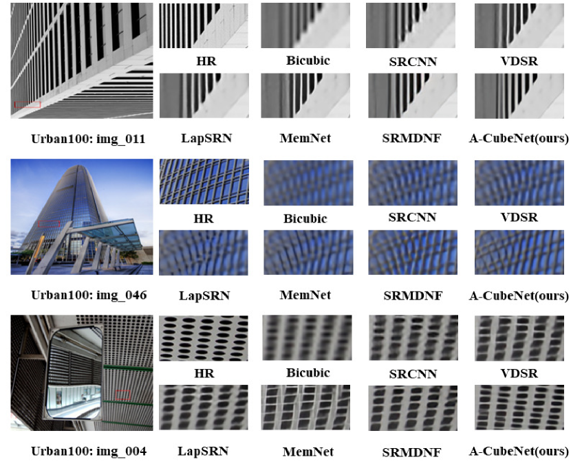
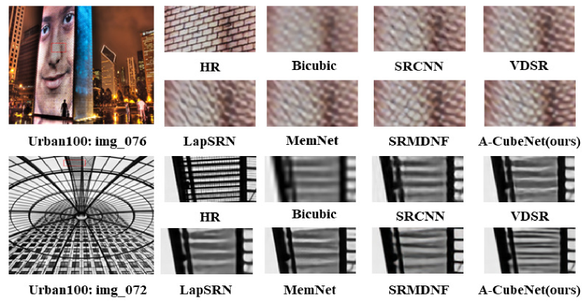
Figure 5. Image super-resolution results with scaling factor $\times$4

Image super-resolution results with scaling factor $\times$4

4.5. Gray Image Denoising

For gray image denosing, we generate the degraded images by adding AWGN noise of different levels (e.g., 10, 30, 50, and 70) to clean images. We compare our A-CubeNet with state-of-the-art gray image denoising methods: BM3D (Dabov et al., 2007), TNRD (Chen and Pock, 2016), DnCNN (Zhang et al., 2017a), MemNet (Tai et al., 2017b), IRCNN (Zhang et al., 2017b), and FFDNet (Zhang et al., 2018c). As shown in Table 5, our A-CubeNet achieves the best PSNR results with all noise levels.

Visual results of different methods under noise level $\sigma=50$ are shown in Figure 6. As shown in Figure 6, BM3D, TNRD, DnCNN, MemNet, IRCNN, and FFDNet can remove noise to some degree, but also over-smooth some details obviously. Compared to these methods, our A-CubeNet not only removes noise well, but also alleviate over-smoothing artifacts obviously because our A-CubeNet covers the information from the whole image and treats different types of information differently.

Table 5. Quantitative results about gray image denoising. Red and blue colors indicate the best and second best performance, respectively.

Method	Kodak24				BSD68
	10	30	50	70	10	30	50	70
BM3D	34.39	29.13	26.99	25.73	33.31	27.76	25.62	24.44
TNRD	34.41	28.87	27.20	24.95	33.41	27.66	25.97	23.83
DnCNN	34.90	29.62	27.51	26.08	33.88	28.36	26.23	24.90
MemNet	-	29.72	27.68	26.42	-	28.43	26.35	25.09
IRCNN	34.76	29.53	27.45	-	33.74	28.26	26.15	-
FFDNet	34.81	29.70	27.63	26.34	33.76	28.39	26.29	25.04
A-CubeNet(Ours)	35.06	29.84	27.77	26.44	33.94	28.50	26.37	25.10

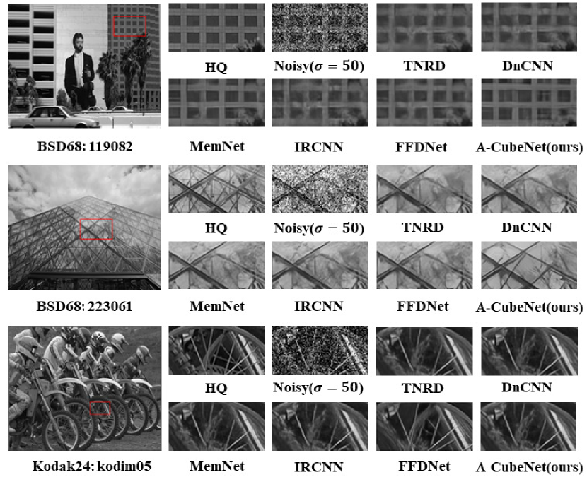
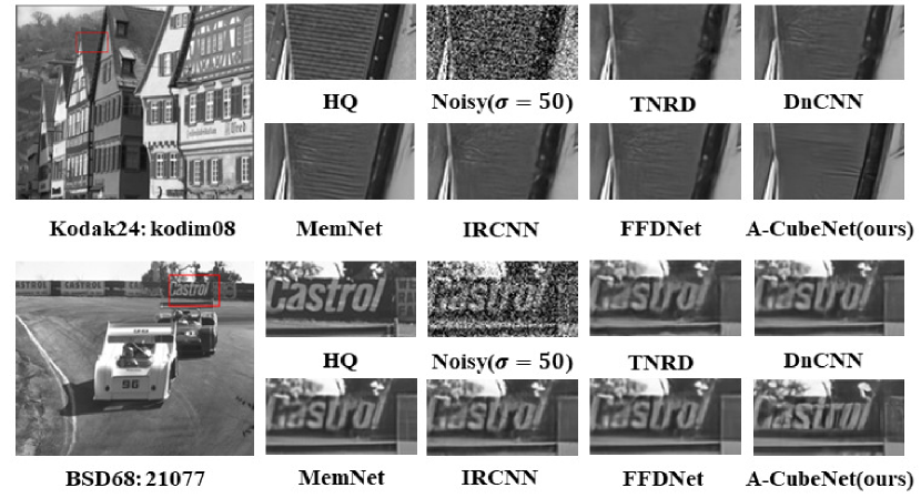
Figure 6. Gray image denoising results with noise level 50

Gray image denoising results with noise level 50

4.6. JPEG Image Deblocking

We also apply our A-CubeNet to reduce image compression artifacts. We use the MATLAB JPEG encoder to generate JPEG deblocking inputs with four JPEG quality settings q = 10, 20, 30, 40. For a fair comparison, we perform training and evaluating both on Y channel of the YCbCr color space. We compare our A-CubeNet with SA-DCT (Foi et al., 2007), ARCNN (Dong et al., 2015a), TNRD (Chen and Pock, 2016), and DnCNN (Zhang et al., 2017a). As shown in Table 6, our A-CubeNet achieves the best PSNR and SSIM results with all JPEG quality settings.

In Figure 7, we also show visual results of different methods. Visual results under very low JPEG quality (q = 10) are provided. As shown in Figure 7, SA-DCT, ARCNN, TNRD, and DnCNN can remove artifacts to some degree, but these methods also over-smooth some details. Compared with these methods, our A-CubeNet not only removes artifacts well, but also preserves more details because our A-CubeNet obtains more details with consistent structures by considering three-dimensional global attention.

Table 6. Quantitative results about JPEG image deblocking. Red and blue colors indicate the best and second best performance, respectively.

Dataset	q	JPEG	SA-DCT	ARCNN	TNRD	DnCNN	A-CubeNet(Ours)
		PSNR/SSIM	PSNR/SSIM	PSNR/SSIM	PSNR/SSIM	PSNR/SSIM	PSNR/SSIM
LIVE1	10	27.77/0.7905	28.65/0.8093	28.96/0.8076	29.15/0.8111	29.19/0.8123	29.54/0.8216
	20	30.07/0.8683	30.81/0.8781	31.29/0.8733	31.46/0.8769	31.59/0.8802	31.93/0.8859
	30	31.41/0.9000	32.08/0.9078	32.67/0.9043	32.84/0.9059	32.98/0.9090	33.35/0.9136
	40	32.35/0.9173	32.99/0.9240	33.63/0.9198	-/-	33.96/0.9247	34.36/0.9289
Classic5	10	27.82/0.7800	28.88/0.8071	29.03/0.7929	29.28/0.7992	29.40/0.8026	29.84/0.8147
	20	30.12/0.8541	30.92/0.8663	31.15/0.8517	31.47/0.8576	31.63/0.8610	32.04/0.8677
	30	31.48/0.8844	32.14/0.8914	32.51/0.8806	32.78/0.8837	32.91/0.8861	33.30/0.8911
	40	32.43/0.9011	33.00/0.9055	33.34/0.8953	-/-	33.77/0.9003	34.16/0.9048

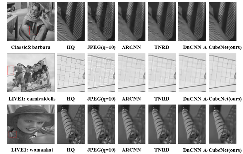
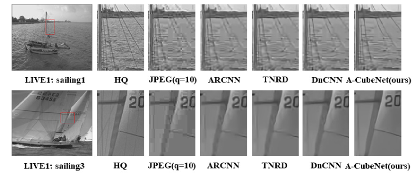
Figure 7. JPEG image deblocking results with JPEG quality 10

JPEG image deblocking results with JPEG quality 10

5. Conclusion

In this paper, we propose a novel attention cube network based on the adaptive dual attention module (ADAM) and the adaptive hierarchical attention module (AHAM) for high-quality image restoration. These two modules constitute the attention cube from spatial, channel-wise and hierarchical dimensions. Our ADAM can capture the long-range contextual information between pixels and channels. As a result, this module successfully expands the receptive field and effectively distinguishes different types of information. Additionally, our AHAM can capture the long-range hierarchical contextual information to combine different feature maps by weights depending on global context. The ADAM and AHAM cooperate to form an ”attention in attention” structure, which is very helpful for image restoration. Our method achieves state-of-the-art image restoration results. In the future, this method will be extended to other image restoration tasks.

- (1)
- Agustsson and Timofte (2017) Eirikur Agustsson and Radu Timofte. 2017. Ntire 2017 challenge on single image super-resolution: Dataset and study. In Proceedings of the IEEE Conference on Computer Vision and Pattern Recognition Workshops (CVPRW). 126–135.
- Ahn et al. (2018) Namhyuk Ahn, Byungkon Kang, and Kyung-Ah Sohn. 2018. Fast, accurate, and lightweight super-resolution with cascading residual network. In Proceedings of the European Conference on Computer Vision (ECCV). 252–268.
- Bevilacqua et al. (2012) Marco Bevilacqua, Aline Roumy, Christine Guillemot, and Marie line Alberi Morel. 2012. Low-Complexity Single-Image Super-Resolution based on Nonnegative Neighbor Embedding. In Proceedings of the British Machine Vision Conference (BMVC). 135.1–135.10.
- Chen and Pock (2016) Yunjin Chen and Thomas Pock. 2016. Trainable nonlinear reaction diffusion: A flexible framework for fast and effective image restoration. IEEE Transactions on Pattern Analysis and Machine Intelligence 39, 6 (2016), 1256–1272.
- Choi and Kim (2017) Jae-Seok Choi and Munchurl Kim. 2017. A deep convolutional neural network with selection units for super-resolution. In Proceedings of the IEEE Conference on Computer Vision and Pattern Recognition Workshops (CVPRW). 154–160.
- Chu et al. (2019a) Xiangxiang Chu, Bo Zhang, Hailong Ma, Ruijun Xu, Jixiang Li, and Qingyuan Li. 2019a. Fast, accurate and lightweight super-resolution with neural architecture search. arXiv preprint arXiv:1901.07261 (2019).
- Chu et al. (2019b) Xiangxiang Chu, Bo Zhang, Ruijun Xu, and Hailong Ma. 2019b. Multi-objective reinforced evolution in mobile neural architecture search. arXiv preprint arXiv:1901.01074 (2019).
- Dabov et al. (2007) Kostadin Dabov, Alessandro Foi, Vladimir Katkovnik, and Karen Egiazarian. 2007. Image denoising by sparse 3-D transform-domain collaborative filtering. IEEE Transactions on Image Processing 16, 8 (2007), 2080–2095.
- Dai et al. (2019) Tao Dai, Jianrui Cai, Yongbing Zhang, Shu-Tao Xia, and Lei Zhang. 2019. Second-order attention network for single image super-resolution. In Proceedings of the IEEE Conference on Computer Vision and Pattern Recognition (CVPR). 11065–11074.
- Dong et al. (2015a) Chao Dong, Yubin Deng, Chen Change Loy, and Xiaoou Tang. 2015a. Compression artifacts reduction by a deep convolutional network. In Proceedings of the IEEE International Conference on Computer Vision (ICCV). 576–584.
- Dong et al. (2014) Chao Dong, Chen Change Loy, Kaiming He, and Xiaoou Tang. 2014. Learning a deep convolutional network for image super-resolution. In Proceedings of the European Conference on Computer Vision (ECCV). 184–199.
- Dong et al. (2015b) Chao Dong, Chen Change Loy, Kaiming He, and Xiaoou Tang. 2015b. Image super-resolution using deep convolutional networks. IEEE Transactions on Pattern Analysis and Machine Intelligence 38, 2 (2015), 295–307.
- Dong et al. (2016) Chao Dong, Chen Change Loy, and Xiaoou Tang. 2016. Accelerating the super-resolution convolutional neural network. In Proceedings of the European Conference on Computer Vision (ECCV). 391–407.
- Foi et al. (2007) A. Foi, V. Katkovnik, and K. Egiazarian. 2007. Pointwise Shape-Adaptive DCT for High-Quality Denoising and Deblocking of Grayscale and Color Images. IEEE Transactions on Image Processing 16, 5 (2007), 1395–1411.
- Guo et al. (2019) Shi Guo, Zifei Yan, Kai Zhang, Wangmeng Zuo, and Lei Zhang. 2019. Toward convolutional blind denoising of real photographs. In Proceedings of the IEEE Conference on Computer Vision and Pattern Recognition (CVPR). 1712–1722.
- Haris et al. (2018) Muhammad Haris, Gregory Shakhnarovich, and Norimichi Ukita. 2018. Deep back-projection networks for super-resolution. In Proceedings of the IEEE Conference on Computer Vision and Pattern Recognition (CVPR). 1664–1673.
- Hu et al. (2018) Jie Hu, Li Shen, and Gang Sun. 2018. Squeeze-and-excitation networks. In Proceedings of the IEEE Conference on Computer Vision and Pattern Recognition (CVPR). 7132–7141.
- Hu et al. (2019) Yanting Hu, Jie Li, Yuanfei Huang, and Xinbo Gao. 2019. Channel-wise and spatial feature modulation network for single image super-resolution. IEEE Transactions on Circuits and Systems for Video Technology (2019).
- Huang et al. (2015) Jia Bin Huang, Abhishek Singh, and Narendra Ahuja. 2015. Single Image Super-resolution from Transformed Self-Exemplars. In Proceedings of the IEEE Conference on Computer Vision and Pattern Recognition (CVPR). 5197–5206.
- Hui et al. (2019) Zheng Hui, Xinbo Gao, Yunchu Yang, and Xiumei Wang. 2019. Lightweight image super-resolution with information multi-distillation network. In Proceedings of the 27th ACM International Conference on Multimedia (ACM MM). 2024–2032.
- Hui et al. (2018) Zheng Hui, Xiumei Wang, and Xinbo Gao. 2018. Fast and accurate single image super-resolution via information distillation network. In Proceedings of the IEEE Conference on Computer Vision and Pattern Recognition (CVPR). 723–731.
- Kim et al. (2016a) Jiwon Kim, Jung Kwon Lee, and Kyoung Mu Lee. 2016a. Accurate image super-resolution using very deep convolutional networks. In Proceedings of the IEEE Conference on Computer Vision and Pattern Recognition (CVPR). 1646–1654.
- Kim et al. (2016b) Jiwon Kim, Jung Kwon Lee, and Kyoung Mu Lee. 2016b. Deeply-recursive convolutional network for image super-resolution. In Proceedings of the IEEE Conference on Computer Vision and Pattern Recognition (CVPR). 1637–1645.
- Kim et al. (2018) Jun-Hyuk Kim, Jun-Ho Choi, Manri Cheon, and Jong-Seok Lee. 2018. Ram: Residual attention module for single image super-resolution. arXiv preprint arXiv:1811.12043 (2018).
- Lai et al. (2017) Wei-Sheng Lai, Jia-Bin Huang, Narendra Ahuja, and Ming-Hsuan Yang. 2017. Deep laplacian pyramid networks for fast and accurate super-resolution. In Proceedings of the IEEE Conference on Computer Vision and Pattern Recognition (CVPR). 624–632.
- Ledig et al. (2017) Christian Ledig, Lucas Theis, Ferenc Huszár, Jose Caballero, Andrew Cunningham, Alejandro Acosta, Andrew Aitken, Alykhan Tejani, Johannes Totz, Zehan Wang, et al. 2017. Photo-realistic single image super-resolution using a generative adversarial network. In Proceedings of the IEEE Conference on Computer Vision and Pattern Recognition (CVPR). 4681–4690.
- Li et al. (2018) Juncheng Li, Faming Fang, Kangfu Mei, and Guixu Zhang. 2018. Multi-scale residual network for image super-resolution. In Proceedings of the European Conference on Computer Vision (ECCV). 517–532.
- Lim et al. (2017) Bee Lim, Sanghyun Son, Heewon Kim, Seungjun Nah, and Kyoung Mu Lee. 2017. Enhanced deep residual networks for single image super-resolution. In Proceedings of the IEEE Conference on Computer Vision and Pattern Recognition Workshops (CVPRW). 136–144.
- Liu et al. (2018a) Ding Liu, Bihan Wen, Yuchen Fan, Chen Change Loy, and Thomas S Huang. 2018a. Non-local recurrent network for image restoration. In Advances in Neural Information Processing Systems (NeurIPS). 1673–1682.
- Liu et al. (2018b) Pengju Liu, Hongzhi Zhang, Kai Zhang, Liang Lin, and Wangmeng Zuo. 2018b. Multi-level wavelet-CNN for image restoration. In Proceedings of the IEEE Conference on Computer Vision and Pattern Recognition Workshops (CVPRW). 773–782.
- Martin et al. (2002) D. Martin, C. Fowlkes, D. Tal, and J. Malik. 2002. A database of human segmented natural images and its application to evaluating segmentation algorithms and measuring ecological statistics. In Proceedings of the IEEE International Conference on Computer Vision (ICCV). 416–423.
- Matsui et al. (2017) Yusuke Matsui, Kota Ito, Yuji Aramaki, Azuma Fujimoto, Toru Ogawa, Toshihiko Yamasaki, and Kiyoharu Aizawa. 2017. Sketch-based manga retrieval using manga109 dataset. Multimedia Tools and Applications (2017).
- Mnih et al. (2014) Volodymyr Mnih, Nicolas Heess, Alex Graves, et al. 2014. Recurrent models of visual attention. In Advances in Neural Information Processing Systems (NeurIPS). 2204–2212.
- Moorthy and Bovik (2009) A. K. Moorthy and A. C. Bovik. 2009. Visual Importance Pooling for Image Quality Assessment. IEEE Journal of Selected Topics in Signal Processing 3, 2 (2009), 193–201.
- Shi et al. (2016) Wenzhe Shi, Jose Caballero, Ferenc Huszár, Johannes Totz, Andrew P Aitken, Rob Bishop, Daniel Rueckert, and Zehan Wang. 2016. Real-time single image and video super-resolution using an efficient sub-pixel convolutional neural network. In Proceedings of the IEEE Conference on Computer Vision and Pattern Recognition (CVPR). 1874–1883.
- Tai et al. (2017a) Ying Tai, Jian Yang, and Xiaoming Liu. 2017a. Image super-resolution via deep recursive residual network. In Proceedings of the IEEE Conference on Computer Vision and Pattern Recognition (CVPR). 3147–3155.
- Tai et al. (2017b) Ying Tai, Jian Yang, Xiaoming Liu, and Chunyan Xu. 2017b. Memnet: A persistent memory network for image restoration. In Proceedings of the IEEE International Conference on Computer Vision (ICCV). 4539–4547.
- Tong et al. (2017) Tong Tong, Gen Li, Xiejie Liu, and Qinquan Gao. 2017. Image super-resolution using dense skip connections. In Proceedings of the IEEE International Conference on Computer Vision (ICCV). 4799–4807.
- Wang et al. (2018) Xiaolong Wang, Ross Girshick, Abhinav Gupta, and Kaiming He. 2018. Non-local neural networks. In Proceedings of the IEEE Conference on Computer Vision and Pattern Recognition (CVPR). 7794–7803.
- Woo et al. (2018) Sanghyun Woo, Jongchan Park, Joon-Young Lee, and In So Kweon. 2018. Cbam: Convolutional block attention module. In Proceedings of the European Conference on Computer Vision (ECCV). 3–19.
- Zeyde et al. (2010) Roman Zeyde, Michael Elad, and Matan Protter. 2010. On Single Image Scale-Up Using Sparse-Representations. In International Conference on Curves and Surfaces (ICCS). 711–730.
- Zhang et al. (2017a) Kai Zhang, Wangmeng Zuo, Yunjin Chen, Deyu Meng, and Lei Zhang. 2017a. Beyond a gaussian denoiser: Residual learning of deep cnn for image denoising. IEEE Transactions on Image Processing 26, 7 (2017), 3142–3155.
- Zhang et al. (2017b) Kai Zhang, Wangmeng Zuo, Shuhang Gu, and Lei Zhang. 2017b. Learning deep CNN denoiser prior for image restoration. In Proceedings of the IEEE Conference on Computer Vision and Pattern Recognition (CVPR). 3929–3938.
- Zhang et al. (2018c) Kai Zhang, Wangmeng Zuo, and Lei Zhang. 2018c. FFDNet: Toward a fast and flexible solution for CNN-based image denoising. IEEE Transactions on Image Processing 27, 9 (2018), 4608–4622.
- Zhang et al. (2018d) Kai Zhang, Wangmeng Zuo, and Lei Zhang. 2018d. Learning a single convolutional super-resolution network for multiple degradations. In Proceedings of the IEEE Conference on Computer Vision and Pattern Recognition (CVPR). 3262–3271.
- Zhang et al. (2018a) Yulun Zhang, Kunpeng Li, Kai Li, Lichen Wang, Bineng Zhong, and Yun Fu. 2018a. Image super-resolution using very deep residual channel attention networks. In Proceedings of the European Conference on Computer Vision (ECCV). 286–301.
- Zhang et al. (2019) Yulun Zhang, Kunpeng Li, Kai Li, Bineng Zhong, and Yun Fu. 2019. Residual non-local attention networks for image restoration. In International Conference on Learning Representations (ICLR).
- Zhang et al. (2018b) Yulun Zhang, Yapeng Tian, Yu Kong, Bineng Zhong, and Yun Fu. 2018b. Residual dense network for image super-resolution. In Proceedings of the IEEE Conference on Computer Vision and Pattern Recognition (CVPR). 2472–2481.