Finite-range viscoelastic subdiffusion in disordered systems with inclusion of inertial effects

Abstract

This work justifies further paradigmatic importance of the model of viscoelastic subdiffusion in random environments for the observed subdiffusion in cellular biological systems. Recently, we showed [PCCP, 20, 24140 (2018)] that this model displays several remarkable features, which makes it an attractive paradigm to explain the physical nature of subdiffusion occurring in biological cells. In particular, it combines viscoelasticity with distinct non-ergodic features. We extend this basic model to make it suitable for physical phenomena such as subdiffusion of lipids in disordered biological membranes upon including the inertial effects. For lipids, the inertial effects occur in the range of picoseconds, and a power-law decaying viscoelastic memory extends over the range of several nanoseconds. Thus, in the absence of disorder, diffusion would become normal on a time scale beyond this memory range. However, both experimentally and in some molecular-dynamical simulations, the time range of lipid subdiffusion extends far beyond the viscoelastic memory range. We study three 1d models of correlated quenched Gaussian disorder to explain the puzzle: singular short-range (exponentially correlated), smooth short-range (Gaussian-correlated), and smooth long-range (power-law correlated) disorder. For a moderate disorder strength, transient viscoelastic subdiffusion changes into the subdiffusion caused by the randomness of the environment. It is characterized by a time-dependent power-law exponent of subdiffusion $\alpha(t)$, which can show nonmonotonous behavior, in agreement with some recent molecular-dynamical simulations. Moreover, the spatial distribution of test particles in this disorder-dominated regime is shown to be a non-Gaussian, exponential power distribution with index $\chi=1.45-2.3$, which also correlates well with molecular-dynamical findings and experiments. Furthermore, this subdiffusion is nonergodic with single-trajectory averages showing a broad scatter, in agreement with experimental observations for viscoelastic subdiffusion of various particles in living cells.

Keywords: anomalous diffusion, viscoelasticity, random environment, non-Gaussian diffusion, non-ergodic features

1 Introduction

Nano- and submicron test particles frequently manifest a subdiffusive behavior on experimentally relevant time scales, which range from picoseconds to hours, in complex polymer and colloidal fluids [1, 2, 3, 4, 5, 6], optically created random potentials [7, 8, 9], cytosol of biological cells [10, 11, 12, 13, 14, 15, 16, 17, 18, 19, 20, 21, 22, 23, 24, 25, 26, 27, 28], biological membranes [29, 30, 31, 32, 33, 34], and DNA tracks [35, 36, 37, 38, 39]. Subdiffusion means that the ensemble-averaged variance of the particles position scales sublinearly in time, $\langle\delta x^{2}(t)\rangle\propto t^{\alpha}$, $0<\alpha<1$. We shall consider a one-dimensional case for simplicity. Typically, $\alpha(t)$ is time-dependent and reaches asymptotically unity, i.e., subdiffusion is a transient phenomenon. However, the pertinent transient time scales can be crucial for physical problems considered. Also conformational diffusion in biological macromolecules such as proteins is often anomalously slow [40, 41, 42, 43, 44, 45, 46, 47, 48, 49]. Different theories were proposed to explain the origin of such subdiffusion based on: (i) continuous-time random walks (CTRWs) [50, 51, 52, 53, 54] with infinite [54, 40, 55, 56, 41, 57, 19] and finite [58, 59, 60] mean residence times (MRTs) in traps and associated fractional Fokker-Planck equation descriptions [61, 54, 62, 59]; (ii) viscoelasticity of the environment [1, 2, 4, 15, 63, 5, 64, 45, 46, 65, 66], or intrinsic viscoelasticity of macromolecules [42, 43, 44, 67, 68, 69] based on a generalized Langevin equation (GLE) description [70, 71, 72, 73], including fractional Langevin equations (FLEs) [74, 75, 67, 68], and fractional Brownian motion (FBM) [76, 77, 78]; (iii) memoryless diffusion in random Gaussian potentials [79, 80, 81, 82, 9, 36, 83]; (iv) normal diffusion coefficient fluctuating in time due to a random environment [84, 27]; (v) diffusion on fractal structures [53], and this is not a complete list [18, 55]. The physical mechanism at play is often controversial, and the experiments are open for concurrent interpretations. For example, the experiments [14] on RNA messengers subdiffusion in E.coli cells were first interpreted in the framework of a CTRW description with infinite MRTs [57]. However, later on, it has been shown that the basic underlying mechanism is viscoelastic and is rather related to FBM [85, 28]. A mixture of different mechanisms can be at play [86, 17, 87]. Moreover, many biological cells are expected to make reversible transitions between a solid-like anabiotic state with frozen metabolic activity, where the CTRW-like mechanism can be more appropriate to a functionally active fluid-like state with viscoelasticity playing a leading role [23].

The viscoelastic nature of subdiffusive processes in the cytosol of biological cells in its functional liquid-like state received a solid experimental support [88, 14, 15, 4, 89, 11, 86, 17, 28, 24, 90, 22]. It was, however, also challenged [57, 19, 91, 56] due to a broad distribution of diffusion coefficients derived from single-trajectory averages because free viscoelastic subdiffusion is ergodic [92, 64, 65, 55]. Hence, diffusion coefficient derived from single-trajectories should not be broadly distributed unless the test particles are broadly distributed in sizes, if diffusion is ergodic. Moreover, the single-trajectory and ensemble averages should coincide. This is, however, frequently not the case. One needs to explain a combination of viscoelastic subdiffusion with non-ergodic features like a large scattering of single-trajectory averages. For living cells, it seems obvious that viscoelastic subdiffusion, as a basic pertinent mechanism, should be combined with trapping caused by elements of the cytoskeleton and molecular crowding. This general idea was until now expressed within three different modeling approaches: (i) by a combination of FBM with CTRW via a subordination, i.e., introducing a randomized time in FBM [86]; (ii) by considering FBM living on a fractal structure [17], and (iii) by considering viscoelastic GLE subdiffusion in random potentials [87] modeling a quenched disorder. The third approach appeals as more physical and fundamental, allowing for various modifications and huge variations, including natural generalizations beyond thermal equilibrium [65].

Indeed, locally memoryless diffusion in disordered media modeled by a random potential or random force-field provides the foundation of several anomalous diffusion theories [93, 52]. For example, the model of CTRW with power-law distributed residence time and divergent MRT in traps comes naturally from the model of exponential energy $U(x)$ disorder with energy fluctuations characterized by a root-mean-square (RMS) amplitude $\sigma=\langle\delta U^{2}(x)\rangle^{1/2}$, yielding $\alpha=k_{B}T/\sigma<1$ for $\sigma>k_{B}T$ [50, 51, 54]. Furthermore, uncorrelated random Gaussian force $f(x)$ model, $\langle f(x)f(x^{\prime})\rangle\propto\delta(x-x^{\prime})$ yields a Brownian motion of the potential $U(x)=-\int^{x}f(x^{\prime})dx^{\prime}$ in space, with growing variance, $\langle\delta U^{2}(x)\rangle\propto x$. It provides a continuous space generalization of the original lattice Sinai model [94] as a Langevin-equation-based subdiffusion in such a fluctuating potential. It yields $\langle\delta x^{2}(t)\rangle\propto|\ln(t/t_{0})|^{a}$ with $a=4$ [93, 95, 96], i.e., a logarithmically slow subdiffusion.

The model of Gaussian energy disorder naturally emerges due to the central limit theorem [93] in many physical systems ranging from organic photoconductors [97, 98] and supercooled liquids [99, 100] to diffusion of regulatory proteins on DNA tracks [101, 102, 103, 104, 105, 36, 37, 38]. Here, Sinai model should be contrasted with the model of uncorrelated or short-range correlated random stationary Gaussian potentials with a finite energy RMS fluctuation, $\sigma$, and normalized autocorrelation function $g(x)=\langle U(x^{\prime}+x)U(x^{\prime})\rangle/\sigma^{2}$, which seems to be more appropriate for such systems. It was, however, long time thought to lead just to normal diffusion with a renormalized diffusion coefficient $D=D_{\sigma=0}\exp[-(\sigma/k_{B}T)^{2}]$ [106, 99, 97, 107]. This theoretical result is known as de Gennes-Bässler-Zwanzig renormalization of diffusion and rate processes by disorder [107]. However, numerical results on the overdamped Langevin diffusion [79, 80, 81, 82, 36, 83] and Monte Carlo jump diffusion [108, 9] revealed a typical subdiffusion even for a short-range correlated disorder, like $g(x)=\exp(-|x|/\lambda)$, on the spatial scale $L_{\rm erg}=2\lambda(k_{B}T)^{2}\exp[(\sigma/k_{B}T)^{2}]/\sigma^{2}\gg\lambda$ [36, 83] strongly exceeding the correlation length $\lambda$, when $\sigma$ exceeds $k_{B}T$ by several times. Also experiments with colloidal particles in optically created random Gaussian potentials confirm the existence of such transient subdiffusion [8, 9]. This subdiffusion occurs paradoxically much faster in absolute terms than the normal diffusion expected from the de Gennes-Bässler-Zwanzig renormalization [36, 83]. Its non-ergodic origin is by now well understood [36, 83]. Remarkably, de Gennes-Bässler-Zwanzig renormalization is mathematically valid asymptotically for any stationary ergodic Gaussian potential with decaying spatial correlations, $g(x)\to 0$, $x\to\infty$ [36]. However, it becomes practically irrelevant and even misleading for $\sigma\gg k_{B}T$. Moreover, strikingly enough, transient subdiffusion emerges also for a potential, which is uncorrelated on the sites of a lattice with a discretization step or lattice period $\Delta x$ and continuous in between [83]. It can also last very long with $\lambda\to\Delta x$ in its spatial range estimate [83].

Another recent surprise was provided by the emergence of a Sinai-like logarithmic diffusion with $b\sim 1-4$ in such stationary Gaussian potentials for $\sigma>5\;k_{B}T$ [83]. All these remarkable features were explained within a simple scaling theory [83] inspired by one developed for the continuous-space Sinai diffusion by Bouchaud at al. [93, 95]. It explains also the origin of a very long transient regime of standard, power-law-scaling ensemble subdiffusion with $\alpha\approx 2k_{B}T/\sigma_{\rm eff}$ and $\sigma_{\rm eff}\approx(1.24-1.52)\sigma$ depending on the model of $g(x)$ [83]. This dependence looks remarkably similar to the case of exponential disorder, and the single-trajectory averages are also broadly scattered. Generally, $\alpha(t)$ is time-dependent, with an extended (for $\sigma>3k_{B}T$) intermediate regime of $\alpha(t)\approx 2k_{B}T/\sigma_{\rm eff}=const$, which turns into a very slow logarithmic increase, $\alpha(t)\sim 2(k_{B}T/\sigma)^{2}\ln(t/t_{0})$, while approaching the asymptotic regime of normal diffusion [83]. For these reasons, we find frequently subdiffusion in random Gaussian potentials in the case of a sufficiently strong disorder, at odds with the outdated dogma of simple renormalization [107]. In this respect, it is pertinent to note that for proteins nonspecifically bound to DNA, disorder strength can reach $\sigma\sim(4-5)\;k_{B}T\sim(0.1-0.125)\;{\rm eV}$ at ambient room $T$ [101, 103, 105], i.e., it is not small at all, contrary to what is often stipulated [102]. To think in terms of normal diffusion with a renormalized diffusion coefficient in such a situation is very misleading [36, 83]. Indeed, for a typical $D_{\sigma=0}=3\;\mu{\rm m^{2}/s}$ [109], $D_{\sigma}\approx 4\times 10^{-5}\;{\rm nm^{2}/s}$ for $\sigma=5\;k_{B}T$, which means that diffusion over 2 nm would take over one day [83]. Subdiffusional search is orders of magnitude faster [36, 37, 38] than this renormalization predicts. In a combination with a local energy bias caused by the disorder correlations [83], this paradoxically fast subdiffusion provides a way to resolve long-standing speed-stability paradox [105]. Such a local energy bias caused by correlated disorder can indeed direct search to a target binding site and greatly accelerate it [104, 83].

The first systematic study of overdamped viscoelastic subdiffusion in random Gaussian potentials was done in Ref. [87] for two fundamental models of correlations: the already mentioned exponentially decaying correlations (Ornstein-Uhlenbeck process in space) and power-law decaying correlations with infinite correlation range. An earlier study was also done in [110] for a peculiar model of $g(x)$ and a weakly corrugated parabolic potential. One of the significant results of [87] is that a small disorder, $\sigma<2\;k_{B}T$, makes an almost negligible impact on viscoelastic subdiffusion on the ensemble level, i.e., viscoelasticity wins over disorder. However, the disorder can introduce a substantial scatter of single-trajectory averages already for $\sigma\sim 1-2\;k_{B}T$. Another significant result is that for a stronger $\sigma>2\;k_{B}T$ disorder such a diffusion starts to look on the ensemble level as diffusion caused by Gaussian disorder (in the absence if viscoelastic memory effects), i.e., the disorder seems to win over viscoelasticity. It can easily be mistaken for diffusion caused by CTRW with divergent MRT [87]. However, residence times are described by a generalized lognormal distribution, and an appropriate scaling time of subdiffusion is expressed through the fractional friction coefficient [87].

In this paper, we include inertial effects in viscoelastic motion [64, 65], which are pertinent, e.g., for subdiffusion in lipid systems [30, 32, 34]. Next, we are looking for a physical explanation of unusual non-Gaussian, exponential power distribution $P(x,t)\propto\exp\left(-|x/x_{\chi}(t)|^{\chi(t)}\right)$ of spreading the test particles positions revealed in viscoelastic subdiffusion in cytosol of living cells [28] ($\chi$ was fixed to the value $\chi=1$ of the Laplace distribution in this paper while fitting the experimental data) and in biological membranes with a generally time-dependent power-law exponent $\chi(t)$ $\chi(t)\sim 1.4-2.2$ [33, 34] and a time-dependent width $x_{\chi}(t)$. We believe that the medium’s disorder causes it. Indeed, Langevin’s memoryless diffusion in Gaussian potentials yields such a distribution with $\chi(t)\sim 1.4-2$; see Fig. 2 of Supplementary Material in [36]. Also experimental distributions of colloidal particle displacements in optically created random Gaussian potentials look similar, cf. Fig. 11 in [8]. For viscoelastic subdiffusion in random Gaussian potentials, it was, however, not studied until now. Next, viscoelastic subdiffusion in pure homogeneous lipid bilayers has a finite time range. For example, for the cases studied in Ref. [32] subdiffusion regime with $\alpha\approx 0.6$ lasted until about 10 ns and then crossed over into normal diffusion. However, in lipid membranes with cholesterol and disordered lipid gel phases, crossover occurs not to normal diffusion but rather to another subdiffusion regime with $\alpha\approx 0.8$ that lasts until 100 ns [32, 34]. It is natural to suppose this regime is due to the medium’s disorder, rather than viscoelasticity, or presents a combination of both.

Moreover, a non-monotonic behavior of $\alpha(t)$ was found in such complex lipid systems crowded besides with proteins [111, 34]. Namely, after reaching a maximum $\alpha(t)$ can drop for a while and then increase again. In this paper, we conceive and investigate a pertinent basic model capable to qualitatively explain these puzzling features as a combination of transient viscoelastic subdiffusion and subdiffusion caused by the disorder.

2 Model and Theory

The model is based on subdiffusion governed by a Kubo-Zwanzig GLE [112, 113, 70, 71]

$$m\ddot{x}+\int_{0}^{t}\eta(t-t^{\prime})\dot{x}(t^{\prime})dt^{\prime}=-dU(x)/dx+\xi(t),$$ (1)

in a zero-mean random stationary Gaussian potential $U(x)$ characterized by a stationary ACF $g(x)$ and RMS $\sigma$. It yields a quenched random force, $f(x)=-dU(x)/dx$. In Eq. (1), $m$ is the mass of a particle, $\eta(t)$ is a frictional memory kernel and $\xi(t)$ is a zero-mean thermal Gaussian noise force, which is completely characterized by its autocorrelation function (ACF) $\langle\xi(t^{\prime})\xi(t)\rangle$. The friction and noise are related by the fluctuation-dissipation relation, $\langle\xi(t^{\prime})\xi(t)\rangle=k_{B}T\eta(|t-t^{\prime}|)$, reflecting thermal fluctuation-dissipation theorem (FDT) [70]. The memory kernel is assumed to have a power law decay, $\eta(t)=\eta_{\alpha}\exp(-\nu_{h}t)/[t^{\alpha}\Gamma(1-\alpha)]$, with an exponential memory cutoff $\nu_{h}$. Here, $\eta_{\alpha}$ is the fractional friction coefficient and $\tau_{h}=1/\nu_{h}$ is a crossover time to normal diffusion, in the absence of quenched random force, $f(x)=0$. Then, the natural time unit is the velocity relaxation time scale $\tau_{v}=(m/\eta_{\alpha})^{1/(2-\alpha)}$ entering the stationary velocity autocorrelation (VACF), which in the limit $\tau_{h}\to\infty$ reads [114, 75, 64, 65]

$$K_{v}(t)=\langle v(t)v(0)\rangle_{\rm st}=v_{T}^{2}E_{2-\alpha}[-(t/\tau_{v})^{2-\alpha}]\;.$$ (2)

It provides a very good approximation within our model for $t\ll\tau_{h}$ and $\tau_{h}\gg\tau_{v}$, which is assumed. Here, $v_{T}=\sqrt{k_{B}T/m}$ is thermal velocity, and $E_{a}(z)=E_{a,b=1}(z)$ is the Mittag-Leffler function, $E_{a,b}(z)=\sum_{n=0}^{\infty}z^{n}/\Gamma(an+b)$. The law of diffusion is given by the twice-integrated VACF,

$$\langle\delta x^{2}(t)\rangle=2v_{T}^{2}t^{2}E_{2-\alpha,3}[-(t/\tau_{v})^{2-\alpha}]\;,$$ (3)

for initial Maxwell distribution of velocities and $t\ll\tau_{h}$. Initially, diffusion is ballistic, $\langle\delta x^{2}(t)\rangle\approx v_{T}^{2}t^{2}$, $t\ll\tau_{v}$. Then, it turns into subdiffusion, $\langle\delta x^{2}(t)\rangle\approx 2D_{\alpha}t^{\alpha}/\Gamma(1+\alpha)$, for $t\gg\tau_{v}$, where $D_{\alpha}$ is the fractional diffusion coefficient obeying a generalized Einstein relation, $D_{\alpha}=k_{B}T/\eta_{\alpha}$, which also expresses FDT. Such a course-grained for $t\gg\tau_{v}$ process is nothing else FBM and this FBM description holds for $\tau_{v}\ll t\ll\tau_{h}$. For $t\gg\tau_{h}$, the normal diffusion regime gradually emerges. In this work, we scale time in units of $\tau_{v}$, velocity in $v_{T}$, length in $x_{0}=v_{T}\tau_{v}$, and energy in $k_{B}T$.

The potential is considered on a lattice with spatial grid size $\Delta x$. It presents randomly generated energy values on the lattice sites, which are continuously connected by parabolic splines, so that that the quenched random force $f(x)$ is piece-wise linear in space [115]. A spectral algorithm for the generation of such a random potential is described in [115]. It was successfully used in many papers and requires to specify some large spurious periodization length $L$ and $g(x)$. We consider three models of correlation decay: (1) $g(x)=\exp(-|x|/\lambda)$ (short-range singular disorder), (2) $g(x)=1/[1+x^{2}/\lambda^{2}]^{\gamma/2}$ with $\gamma=1$ and $g(x)\sim(\lambda/|x|)^{\gamma}\;{\rm at}\;x\gg\lambda$ (long-range non-singular disorder with diverging correlation length), and (3) $g(x)=\exp(-x^{2}/\lambda^{2})$ (short-range non-singular disorder) for two values $\lambda=10$ and $\lambda=100$. The model of power-law correlated disorder with $\gamma=1$ emerges due to a charge-dipole interaction, e.g., in the context of charge diffusion in molecularly doped polymers [98], where typically $\sigma\sim 4$ in units of room $k_{B}T_{r}\sim 0.025$ eV. The electrostatic nature of this model of correlated disorder qualifies it as an important physical model. The models of exponentially correlated disorder (Ornstein-Uhlenbeck process in space) and Gaussian correlations are basic models of generic interest. Exponential correlations lead to a singular model, while a Gaussian decay provides a non-singular model of short-range correlations. Typical realizations of corresponding random potentials are shown in Fig. 1. Notice a very rugged character of potential fluctuations in the case of exponential correlations and a strong local bias on a typical scale of $\lambda$ in the cases of exponential and power-law correlations. In this respect, the character of a smooth disorder is not changed upon making $\Delta x$ ever smaller, provided $\Delta x\ll\lambda$: there are typically about one or two local potential minima per $\lambda$ length. The Ornstein-Uhlenbeck process in space (exponential correlations) is very different: there are huge many local minima and maxima within its correlation length and their number increases upon diminishing $\Delta x$. Indeed, this process can only be defined on a lattice with some finite $\Delta x$ given its singular character because for this process the force RMS $\langle f^{2}(x)\rangle^{1/2}=\sigma\sqrt{2/(\Delta x\lambda)}\to\infty$ diverge with $\Delta x\to 0$ [36, 83, 87]. Power-law-decaying and Gauss-decaying correlations yield smooth $U(x)$ [83, 87]. In these cases, $\langle f^{2}(x)\rangle^{1/2}=\sqrt{2}\sigma/\lambda$, and $\langle f^{2}(x)\rangle^{1/2}=\sqrt{\gamma}\sigma/\lambda$, respectively, when $\Delta x\to 0$.

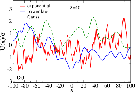
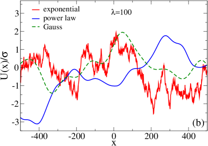
Figure 1: Realizations of random potentials for exponential, power-law with $\gamma=1$, and Gauss-decaying correlations. The lattice grid size is $\Delta x=1$. (a) $\lambda=10$; (b) $\lambda=100$. $L=2^{19}\Delta x\approx 5.24\times 10^{5}$.

Since the analytical treatment of diffusion and transport processes of strongly non-Markovian GLE dynamics in random correlated potentials is not feasible, we investigated it numerically.

2.1 Numerical approach

The numerical approach is based on approximating the memory kernel by a sum of exponentials and a hyper-dimensional Markovian embedding of the low-dimensional GLE dynamics. It is very well developed both in application to sub-diffusive [64, 65, 87] and super-diffusive GLE [116, 117, 118], including FLE dynamics. This numerically accurate approach is detailed in A.

2.2 Ensemble vs. trajectory averages, ergodicity and its breaking

Notice that ergodicity of random processes can be understood in various senses [119], with ergodicity in the mean value serving as the basic central notion [119]. The ergodicity of a diffusion process $x(t)$ is considered in the current literature as ergodicity of $x(t)$ in its squared increments [55]. Namely, it is considered as a mean-value ergodicity of the stochastic process defined by the squared position increments, $[\delta x_{i}(t|t^{\prime})]^{2}$, of $x(t)$ within some time interval $t$, where $\delta x_{i}(t|t^{\prime})=x_{i}(t^{\prime}+t)-x_{i}(t^{\prime})$. Here, $t^{\prime}$ is the running time of this process and $t$ is a forward time-increment of the $i$-th trajectory counted from this running time. The time-average of these squared position increments over $t^{\prime}$ is defined as $\overline{\delta x_{i}^{2}(t)}^{{\cal T}_{w}}=\frac{1}{{\cal T}_{w}-t}\int_{0}^{{\cal T}_{w}-t}[\delta x_{i}(t|t^{\prime})]^{2}dt^{\prime}$, i.e., as a running trajectory average within a time window $\Delta{\cal T}_{w}={\cal T}_{w}-t\gg t$. It depends on $t$ and ${\cal T}_{w}$. In 1d, the single-trajectory diffusion coefficient, $D_{i,\rm sgl}$, is defined by scaling $\overline{\delta x_{i}^{2}(t)}^{{\cal T}_{w}}\sim 2\bar{D}_{i,\rm sgl}({\cal T}_{w})t^{\alpha}$ with growing $t$. Often, the definition involves an additional gamma-function factor $\Gamma(1+\alpha)$, $\bar{D}_{i,\rm sgl}({\cal T}_{w})=D_{i,\rm sgl}({\cal T}_{w})/\Gamma(1+\alpha)$, which we will, however, not use for the single-trajectory averages. The empiric ensemble averaging presents a more common concept, $\langle\delta x^{2}(t)\rangle_{M}=(1/M)\sum_{i=1}^{M}[\delta x_{i}(t|t^{\prime})]^{2}$, and the ensemble diffusion coefficient, $D_{M,\alpha}$, is defined by $\langle\delta x^{2}(t)\rangle_{M}\sim 2\bar{D}_{M,\alpha}t^{\alpha}$. $M$ will be mostly omitted in the following while assuming that is sufficiently large. Moreover, $t^{\prime}$ is set to zero in the corresponding ensemble averages, while sampling initial particles positions randomly in space. Notice that only for the stationary in wide sense increments this average does not depend on $t^{\prime}$. Diffusion is considered ergodic if both averages exist and coincide, $\overline{\delta x_{i}^{2}(t)}^{\infty}=\langle\delta x^{2}(t)\rangle_{\infty}$, in the limit $\Delta{\cal T}_{w}\to\infty,M\to\infty$. From a mathematical point of view, these averages can be identical only for processes with stationary increments. Otherwise, they cannot be expected to coincide [119, 120]. Nevertheless, from a physical point of view both averages always make sense and should be considered different and mutually complementary characteristics of diffusion processes. Evidently, they are not expected to ever coincide in disordered media with quenched disorder, where the position increment for any particular trajectory is never stationary.

By Khinchin theorem [119, 120], a sufficient condition for ergodicity of a stationary random process in the mean value is the decay of its ensemble stationary autocorrelation function (ACF) to zero (in the limit $M\to\infty$, which is equivalent to the ensemble-averaging in a proper mathematical sense using the probability density function). Slutsky’s theorem poses an even weaker condition: it is necessary and sufficient that the time-average of the stationary ensemble ACF decays to zero in the limit of infinite averaging interval [119, 120]. For the discussed ergodicity of diffusion processes, a more complex sufficient condition necessarily emerges, and it can be formulated in terms of four-points correlation functions of increments [119]. However, for Gaussian processes, it reduces to decay of the (infinite) ensemble autocorrelation function of increments to zero [119, 120]. It is the case of FBM (a singular non-differentiable stochastic process with stationary increments) and its inertial generalization [92, 64] based on GLE, including FLE, with a well defined (by contrast with FBM) velocity $v(t)=\dot{x}(t)$. We consider it in this paper as a basic process, which is ergodic in the absence of an external potential. However, when a trapping (e.g., bistable) potential is present, the limit of sufficiently large $t^{\prime}\to\infty$ must be considered. Otherwise, both averages can never coincide even for perfectly ergodic processes, requiring some relaxation time to reach a stationary limit within a potential trapping domain. This is also the reason why a mean-ergodic, or even correlation-ergodic process can be profoundly non-ergodic, e.g., from the viewpoint of statistics of transitions between two trapping subdomains [121, 69, 68]. different from one expected from the relaxation dynamics in such trapping domains. In such a case, swift transitions between two trapping domains can occur in the background of a slow relaxation dynamics within the whole domain of bistability [64, 65, 69]. Here, the main preconditions of the rate theory [107] are violated, and, nevertheless, it can remain useful and predictive, to a certain extent [64, 65, 48]. In periodic potentials, such an inertial generalization of FBM is also asymptotically ergodic [64]. However, the pace of establishing this ergodic asymptotics heavily depends on the potential amplitude in units of the thermal energy $k_{B}T$, and this asymptotics is not necessarily achievable in practice [64]. These remarks already explain why viscoelastic subdiffusion in complex environments is generally not ergodic, and a scatter of single-trajectory averages does not contradict the viscoelastic nature of subdiffusion in complex inhomogenous fluids, including cytosol of biological cells.

On the practical level, we neither ever have infinitely long trajectories nor infinitely large ensembles. Hence, both averages never coincide empirically exactly even for ergodic process. However, for a genuinely ergodic process, they do agree well for sufficiently large $\Delta{\cal T}_{w}\gg t$ and $M\gg 1$, which is the case of FBM and potential-free GLE subdiffusion [92, 64, 65, 55]. For this, however, $\Delta{\cal T}_{w}$ must exceed $t$ by a factor of at least 100. Notice that some authors consider even ${\cal T}_{w}\sim t$ or $\Delta{\cal T}_{w}\sim 0$ in discussion of ergodic properties [55]. It makes, strictly speaking, a little sense in this context. This point is crucial because most of the existing thus far experimental confirmations of aging in anomalous diffusion in living cells have ${\cal T}_{w}$, which at best is only one hundred times larger than the corresponding $t$. Such proofs lack a profound statistical significance, especially considering that also $M$ is, at best, several hundred in most experiments, as we discuss below in the context of our model.

3 Results and Discussion

3.1 Ensemble averages

We first performed calculation of the ensemble averages with $M=10^{5}$ particles in each case (cf. A for pertinent details) using three models of correlation decay and two values of $\lambda=10$ and $\lambda=100$. The memory kernel approximation is chosen in such a way that FLE subdifussion with $\alpha=0.6$ should last in the absence of potential until about $t=10^{3}$. Then, it gradually changes into asymptotically normal diffusion, see the cases of free diffusion in Figs. 2, 3 (a). This behavior is convenient to characterize by a time-dependent power law exponent $\alpha(t)=d\ln\langle\delta x^{2}(t)\rangle/d\ln t$, see in Figs. 2, 3 (b). Initially it is always ballistic, $\alpha=2$, $\langle\delta x^{2}(t)\rangle\approx(v_{T}t)^{2}$, given initially thermally distributed velocity variable in this work. Then, after some transient an FBM regime with $\alpha_{\rm eff}\approx 0.6$ establishes for $t\geq 10$ and lasts until $t\sim 10^{3}-10^{4}$. Then, significant deviations from $\alpha=0.6$ start. The power exponent grows and the regime of normal diffusion gradually establishes until the end of simulations at $t_{\rm max}=10^{7}$. This behavior strongly reminds one for diffusion of lipids in 1,2-Distearoyl-sn-glycero-3-phosphocholine (DSPC), 1-stearoyl-2-oleoyl-sn-glycero-3-phosphocholine (SOPC), and 1,2-Dioleoyl-sn-glycero-3-phosphocholine (DOPC) lipid bilayers in [32, 34], see Fig. 8 in [34]. Therein, FBM and FLE subdiffusive regime with $\alpha=0.6$ lasts until about 10 ns and then changes gradually into normal diffusion. With $\tau_{v}=0.323$ ps (B), our $t=10^{4}$ corresponds to 3.23 ns and $t=10^{7}$ to 3.23 $\mu$s.

The presence of a random potential radically changes this simple picture. Within the time-range of purely viscoelastic subdiffusion ($t<10^{3}$) disorder practically does not influence it on the ensemble level, see in Figs. 2, 3, (a). It is especially surprising for a very rough exponentially correlated disorder with $\lambda=10$ and $\sigma=2$ in Fig. 2 (a) (see a typical realization of such a disorder in Fig. 1 (a)), and also for a power-law correlated disorder for $\sigma=4$ and $\lambda=10$. Naive expectation based on the de Gennes-Bässler-Zwanzig renormalization is that the diffusional spread should be suppressed by the factor $\exp[-\sigma^{2}/(k_{B}T)^{2}]$, which is approximately $0.01832$ for $\sigma=2$ and $1.12535\times 10^{-7}$ for $\sigma=4$. However, this expectation is not justified; see in Fig. 2 (a). Time-dependent $\alpha(t)$ shows some dynamics in Fig. 2 (b). However, changes on the level of $\langle\delta x^{2}(t)\rangle$ are not easy to detect in part (a). This striking feature was described earlier within a bit different model (no inertial effects, diffusion is initially normal due to a normal friction component in GLE) in [87]. Also, in periodic potentials, GLE subdiffusion is asymptotically insensitive to the presence of potential [64, 65]. For a sinusoidal potential, it can be even proven rigorously within a quantum-mechanical setting while considering the sub-Ohmic model of generalized Brownian motion [114], which corresponds to the considered viscoelastic GLE subdiffusion [65]. In periodic potentials, however, transient effects can last very long, depending on the potential amplitude [64, 65]. In the present case, no related transients can be seen on the ensemble level, even for $\sigma=4$ in Fig. 2 (a), which is quite surprising. The influence on the level of single-trajectory averages is, however, in the case $\lambda=10$, profound, see below. Next, transition to normal diffusion regime does not occur until $t_{\rm max}=10^{7}$. A new anomalous diffusion regime caused by disorder is gradually established for $t>10^{5}$, with vibrant transient features, which depend on the type of correlation decay, $\sigma$, and $\lambda$.

Indeed, for exponential correlations and $\sigma=2$, $\alpha(t)\approx 0.55-0.57<0.6$ for $t=10^{2}-10^{4}$ in Fig. 2 (b) (full red line therein). For $t>10^{4}$ it starts to grow slowly and reaches $\alpha\approx 0.774$ at $t=3.2\times 10^{6}$. In this respect, it is worth noting that in the case of overdamped normal diffusion in such a potential, $\alpha(t)$ reaches a minimal value $\alpha\approx 0.70$ [36, 83] before it starts to grow logarithmically slow in time until unity. We expect such a slow growth also in the case under study. However, the asymptotic regime of normal diffusion is numerically out of reach. Also in the case of Gaussian correlation decay, $\alpha(t)$ first drops slightly below $0.6$, reaching its minimum $\alpha_{\rm min}\approx 0.50$ at $t\approx 2\times 10^{3}$ and then slowly grows until $\alpha\approx 0.77$ at $t=3.2\times 10^{6}$. Especially interesting is the case of power-law correlations with divergent correlation length because in this case subdiffusion caused by the correlated Gaussian disorder alone (without viscoelastic memory effects) is the longest [83]. In this case, $\alpha(t)$ stays close to $0.6$ for $t$ between $10$ and $10^{5}$. Then, it grows and stays nearly constant $\alpha(t)\approx 0.72$ from $t=10^{6}$ till the end of the simulations. In this respect, $\alpha\approx 0.70$ is about the minimal value of transient subdiffusion caused also by Gaussian power-law correlated disorder [83]. In the case of normal overdamped diffusion in considered random potentials, the spatial range of nonergodic transient subdiffusion is determined by a nonergodicity length $L_{\rm erg}$, which is a typical length scale, where the statistical weight function $w(x)=\exp[-U(x)/(k_{B}T)]$ lacks self-averaging [36, 83]. For $\sigma=2$, $L_{\rm erg}\approx 35\lambda$ in the case of exponential correlations, $L_{\rm erg}\approx 52\lambda$ in the case of Gauss-decaying correlations, and $L_{\rm erg}\approx 167\lambda$ in the case of power-law decaying correlations with $\gamma=0.8$, see Table I in [83]. Hence, in the case of power-law correlations (here $\gamma=1$ vs. 0.8 in [83]) one can expect that subdiffusion will last at least until about $\delta x\sim 1.67\times 10^{3}x_{0}$ for $\lambda=10$ and $\delta x\sim 1.67\times 10^{4}x_{0}$ for $\lambda=100$, which for $x_{0}=0.026$ nm (B) would correspond to 43.42 nm and 434.2 nm, correspondingly. With increasing $\sigma$, $L_{\rm erg}$ grows super-exponentially fast. Already for $\sigma=4$, $L_{\rm erg}\sim 10^{6}\lambda$ for a short-range correlated disorder [83]. Then, the corresponding nonergodicity length reaches practically a macroscale, $L_{\rm erg}\approx 0.26$ mm and $2.6$ mm at $\lambda=10$ and $\lambda=100$, correspondingly. In this respect, the case of power law correlation in Fig. 2 with $\sigma=4$ is interesting. From $t=10^{4}$ on in part (b), $\alpha(t)\sim 0.44-0.47$ with $\alpha_{\rm min}\approx 0.44$ at the end of simulations, where it seems to slightly decline further. It agrees well with $\alpha_{\rm min}\approx 0.43$ for power-law correlations in Fig. 3 (b) of Ref. [83] obtained for memoryless diffusion.

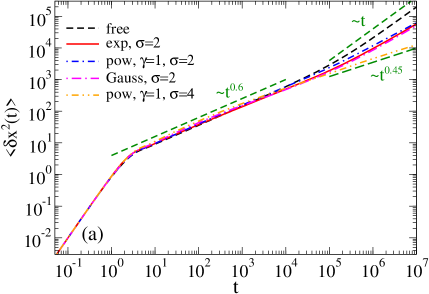
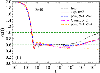
Figure 2: (a) Ensemble-averaged mean-square displacement vs. time for several models of correlation decay (exponential, power-law with $\gamma=1$, and Gaussian) at $\lambda=10$ and several values of disorder strength $\sigma$ shown in the plot. (b) Dependence of power-law exponent $\alpha(t)$ on time corresponding to (a).

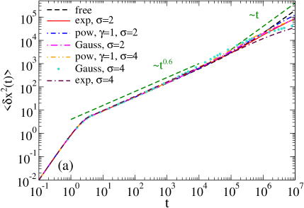
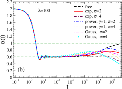
Figure 3: (a) Ensemble-averaged mean-square displacement vs. time for several models of correlation decay (exponential, power-law with $\gamma=1$, and Gaussian) at $\lambda=100$ and several values of disorder strength $\sigma$ shown in the plot. (b) Dependence of power-law exponent $\alpha(t)$ on time corresponding to (a).

The case of $\lambda=100$ in Fig. 3 is interesting for some lipid-proteins systems. For such a large $\lambda$ and a smooth disorder, the time range of viscoelastic diffusion is restricted virtually by motion within one local minimum of the random potential, cf. Fig. 1 (b), of a typical spatial size $\lambda$. In this case, $\alpha(t)$ dynamics in Fig. 3 (b) shows an interesting novel non-monotonic feature in all studied cases. Namely, it first starts to grow, like in the potential-free case. However, after a maximum is reached, $\alpha(t)$ drops. For example, for exponential correlations (in this singular case, a very rough multiple-extrema structure of potential holds also on a spatial scale much smaller than $\lambda$) and $\sigma=2$, $\alpha_{\rm max}(t)\approx 0.763$ is reached at $t=5.4\times 10^{5}$. After this, it drops to $\alpha(t)\approx 0.717$ at $t=3.17\times 10^{6}$. Given the results in [83], one can predict that it will further drop to $\alpha\approx 0.70$ and then start to grow logarithmically slow to the asymptotically normal value. Furthermore, for Gauss-decaying correlations and $\sigma=2$, $\alpha_{\rm max}(t)\approx 0.760$ is reached at $t=2.84\times 10^{5}$, and it drops to $\alpha(t)\approx 0.648$ at $t=3.17\times 10^{6}$. For this model of the disorder, $\alpha_{\rm min}\approx 0.6$, see in Fig. 3 (d) in [83]. Hence, it is expected that with increasing time, it will drop further to this minimum value and then gradually increase to the asymptotically normal value. In case of power-law correlations and $\sigma=2$, $\alpha_{\rm max}(t)\approx 0.842$ is reached at $t=5.57\times 10^{5}$, and it drops to $\alpha(t)\approx 0.768$ at $t=3.17\times 10^{6}$. One expects that it will further drop to $\alpha_{\rm min}=0.70$ and then gradually grow. Interestingly, a reminiscent nonmonotonous behavior of $\alpha(t)$ was found both for lipids and proteins in MD simulations of disordered lipid-protein systems, see Figs. 15, 16 in [34], and references therein.

Next, for $\sigma=4$ and exponential correlations, $\alpha_{\rm min}\approx 0.375$ in the case of normal diffusion [36] (see inset in Fig. 1 therein) and it can stay for a very long time nearly constant. In Fig. 3 (b), the minimal value reached at $t=3.17\times 10^{6}$ for exponential correlations is $\alpha\approx 0.456$. The true minimum is hence still not reached. For power-law correlations in this figure, the minimum at the end of simulations is $\alpha\approx 0.529$. It is well above the expected minimal $\alpha_{\rm min}\approx 0.43$, which is still not reached. Also, for Gaussian correlations, $\alpha\approx 0.406$ at the end is still above the expected minimum. After it will be reached, $\alpha(t)$ is expected to stay nearly constant for a long time and then logarithmically slow grow until unity. These predicted features are, however, beyond any numerical study currently possible.

It must be emphasized that in our estimations we tacitly assume that on the time scale exceeding the long-time cutoff of the memory kernel $\tau_{h}$ we can think in terms of normal diffusion with an effective friction coefficient $\eta_{\rm eff}=\int_{0}^{\infty}\eta(t)dt$, which takes place in a random potential. The validity of this assumption should be checked in the subsequent research. One cannot exclude that a synergy of viscoelastic memory effects and nonergodic effects due to the randomness of potential will tremendously increase nonergodicity length.

3.2 Distribution of particle positions

A very intriguing question emerges on the origin of the exponential power distribution

$$P(x,t)\propto\exp\left(-|x/x_{\chi}(t)|^{\chi(t)}\right)\;.$$ (4)

Such a distribution is commonly found in viscoelastic biological subdiffusion, e.g., for RNA-protein complexes in various cells with a fixed power exponent $\chi=1$ in Ref. [28]. Furthermore, crowded protein-lipid systems also display this distribution with $\chi=1.4-1.6$ [33, 34]. Very important in this respect is that normal diffusion in disordered Gaussian potentials typically displays this distribution with a time-dependent $\chi(t)$, see Fig. 2 of Supplemental Material in Ref. [36], where $\chi\sim 1.4-1.6$ for $\sigma=2-4$. Hence, it is expected that the viscoelastic subdiffusion of a restricted temporal range in Gaussian potentials will display this striking feature.

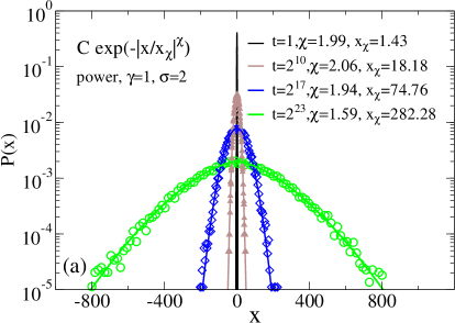
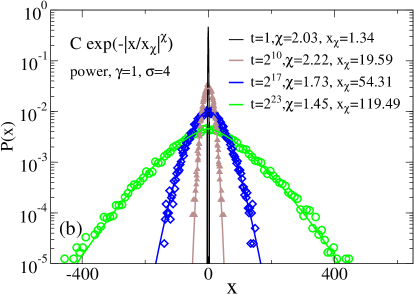
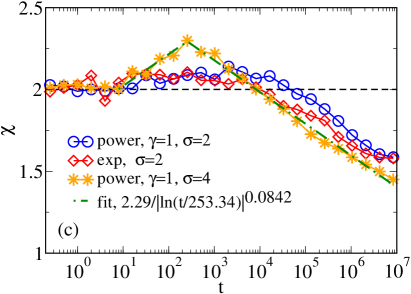
Figure 4: Distribution of particle positions for several values of time in the case of power-law correlations with $\gamma=1$, $\lambda=10$ and (a) $\sigma=2$, (b) $\sigma=4$. Symbols display the numerical results and lines the corresponding fits with Eq. (4) and parameters shown in plots. Panel (c) displays time-dependence $\chi(t)$ for several models of correlations with $\lambda=10$, and a fit with (5) in one case.

Indeed, our simulations in Fig. 4 confirm this expectation. They reveal the following common features. Initial delta-distribution spreads first approximately as a Gaussian, $\chi=2$, see in panel (c). Then, during the viscoelastic stage, $\chi$ fluctuates around $\chi=2$, and can even reach $\chi\approx 2.3$, see the case of power-law correlations in panel (c). It drops below $\chi=2$, beyond the temporal range of viscoelastic correlations, where the very occurrence of subdiffusion is on the count of the randomness of potential. For $\sigma=2$, $\chi(t)$ relaxes down to $\chi_{\rm min}\approx 1.59$ for several models of correlations under study, see in panel (a) for power-law correlations. For $\sigma=4$, the minimal value of $\chi$ in parts (b), (c) is $\chi=1.45$. However, the real minimum, in this case, is still not achieved until the end of the simulations. The relaxation law is inverse logarithmic

$$\chi(t)\propto 1/[\ln(t/t_{c})^{r}]$$ (5)

with $t_{c}\approx 253.34$ and $r\approx 0.0842$ for $\sigma=4$ in the case of power-law correlations, see in Fig. 4 (c). After reaching the minimum, it is expected that $\chi$ will stay nearly constant for a while and then it will gradually increase to $\chi=2$ asymptotically, while the normal diffusion limit will gradually be achieved. To realize this feature, see the case $\sigma=1$ in the inset of Fig. 2 of Supplemental Material in Ref. [36]. In the case $\lambda=100$, the relaxation behavior in Fig. 4 (c) is shifted to the right (not shown). For example, for $\sigma=2$ and power-law correlations, $\chi\approx 1.736$ at the end of the simulations, and for $\sigma=4$ it arrives at $\chi\approx 1.704$, i.e., indeed $\chi_{\rm min}$ is still far from being reached in both cases.

3.3 Trajectory averages

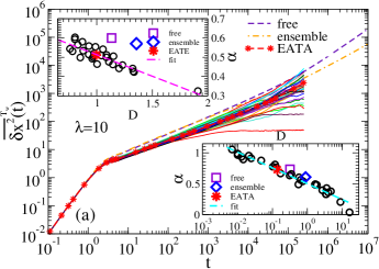
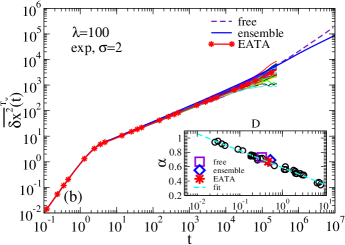
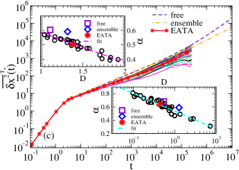
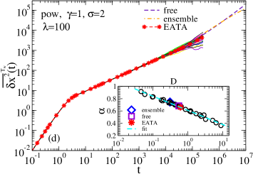
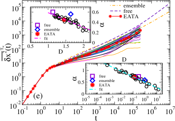
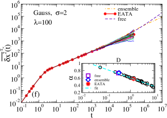
Figure 5: Single-trajectory averages for (a,b) exponential correlations, (c,d) power-law correlations with $\gamma=1$, (e,f) Gauss-decaying correlations for $\sigma=2$ and two values $\lambda=10$ (a,c,e) and $\lambda=100$ (b,d,f). In each case, 30 trajectory averages are displayed. They are to compare with the ensemble averages in the cases of free diffusion and for the specific potential disorder also shown. Besides, ensemble-averaged time-averages (EATAs), $\left\langle\overline{\delta x_{i}^{2}(t)}^{{\cal T}_{w}}\right\rangle$ are shown in each case. Upper insets in (a,c,d) show pairs $(D,\alpha)$ derived from the fits of single-trajectory averages by $2Dt^{\alpha}$ within the time-interval $[10,10^{3}]$. Lower insets in (a,c,d) show the corresponding pairs derived from the fits within the time-interval $[10^{3},2\times 10^{5}]$. In (b,d,f) the corresponsing fits are done within the time-interval $[10,2\times 10^{5}]$. Straight lines in upper insets display the best fits of numerical data with Eq. (7). Straight lines in lower insets display best fits with Eq. (6). In both cases, fitting parameters are given in Table 1.

Next, we proceed with studying single-trajectory averages, which are of special interest because disorder generally implies a broken ergodicity. For this, we use ${\cal T}_{w}=2\times 10^{6}$ and evaluate single-averages until $t_{\rm max}=0.1{\cal T}_{w}$. The results are shown in Fig. 5 for $\sigma=2$, three models of correlation decay and two values of $\lambda$. Consider first the case $\lambda=10$ in parts (a,c,e). First of all, in the initial regime, $t<2$, (including thermal ballistic diffusion), self-averaging occurs for every trajectory. No scatter is present. In this regime, ensemble and trajectory averages coincide. Thus, diffusion is ergodic. For $t>2$ in the cases of exponential and Gaussian correlations and $t>10$ for power-law correlations, the scatter becomes visible. It is noticeable that it becomes enhanced for $t>10^{3}$, beyond the range of viscoelastic memory effects. Hence, we consider two different time intervals (i) $[10,10^{3}]$ and (ii) $t>10^{3}$ to characterize diffusional properties with a pair of random variables $(D,\alpha)$ for each separate trajectory defined on the corresponding time intervals. The results are depicted in upper and lower insets in parts (a,c,e), correspondingly. They display a striking feature. Namely, while one of the variables can be considered completely random, another is tightly related by

$$D(\alpha)=D_{0}e^{-(\alpha-\alpha_{0})/\alpha_{1}},$$ (6)

or $\alpha(D)=\alpha_{0}-\alpha_{1}\ln(D/D_{0})$ in the case of a strong scatter, see lower insets in Fig. 5, (a-f), with $D_{0},\alpha_{0},\alpha_{1}$ in Table I. In other words, $D$ and $\alpha$ are strongly (anti-)correlated. Interestingly, variations of the parameter $\alpha_{1}$ are rather small, $\alpha_{1}\approx 0.100-0.116$, while variations of $D_{0}$ and $\alpha_{0}$ are significant reflecting the model of correlations and $\lambda$. Values of $D$ are scattered over three orders of magnitude in the case of exponential and power-law correlations, and even four (!) orders, in the case of Gaussian correlations. It comes as a surprise that the largest scatter appears in the case of Gaussian correlations, where the random potential is smooth and shows the least local bias because of very short-range correlations, see panel (e) in Fig. 5.

Furthermore, for a smaller scatter, $|\alpha-\alpha_{0}|\ll\alpha_{1}$, (6) yields

$$\alpha(D)=\alpha_{2}-b_{1}D$$ (7)

with $\alpha_{2}=\alpha_{0}+\alpha_{1}$, $b_{1}=\alpha_{1}/D_{0}$. Indeed, the upper insets in Fig. 5, (a,c,e) display such a linear dependence for $10<t<1000$, however, with $\alpha_{2},b_{1}$, which are not related to $\alpha_{0},\alpha_{1},D_{0}$, see in Table 1.

Next, the ensemble-averaged time-averaged (EATA) variance of particle positions lies essentially below the corresponding ensemble-averaged variance, cf. Fig. 5 (a,c,e). Also the corresponding values of $\alpha$ are different. For example, in the upper inset in (a), $\alpha_{\rm EATA}\approx 0.512$ for EATA, while $\alpha\approx 0.571$ for the ensemble-average therein. Likewise, in the lower inset (a), $\alpha_{\rm EATA}\approx 0.727$ for EATA and $\alpha\approx 0.608$ for the ensemble-average. Interestingly, a very similar feature, i.e., a small scatter in viscoelastic FBM regime ($t<10$ ns) with $\alpha_{\rm EATA}\approx 0.52-0.54$ and a strong scatter with $\alpha_{\rm EATA}\approx 0.79-0.82$ was revealed in a DSPC lipid-cholosterol mixture in Ref. [32], see also Fig. 10 in review [34].

Table 1: Parameters of fit in Fig. 5

• Panel	$\alpha_{0}$	$\alpha_{1}$	$D_{0}$	$\alpha_{2}$	$b_{1}$
  a	0.2875	0.1112	6.7742	0.7364	0.2230
  b	0.7269	0.1022	0.2560
  c	0.3082	0.1161	7.1809	0.7959	0.2086
  d	0.5833	0.1000	1.2907
  e	0.6410	0.1007	0.2546	0.8725	0.2854
  f	0.4717	0.1024	3.60887

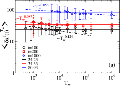
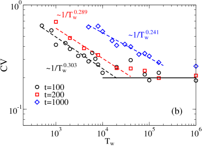
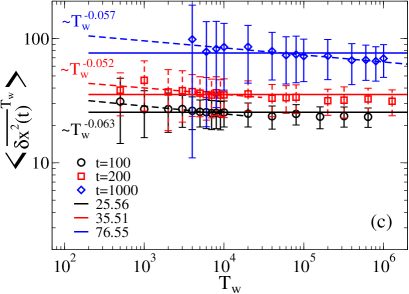
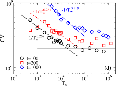
Figure 6: Dependence of EATA on averaging time-window ${\cal T}_{w}$ for three values of $t=100,200,1000$ in the case of $\sigma=2$ for (a) exponential correlation and (b) Gaussian correlations. Panels (b) and (d) show the time-dependence of the corresponding coefficients of variation (CVs) of the time-averages. The ensemble average over $M=200$ single-trajectory averages is done in each case. Notice that a very weak “aging” in parts (a,c) occurs only until ${\cal T}_{w}\sim 100t$, see the corresponding dashed lines $\sim 1/{\cal T}_{w}^{a}$, with power exponents $a$ shown in (a,c). Hence, this is not genuine aging, but rather a transient statistics effect. The best fits with constants (full lines) shown in (a,c) look almost perfect, upon taking error bars into account. Also, CVs power-law decay with exponent $a$ shown in (b,d) until ${\cal T}_{w}$ reaches about $100t$ in each case. After this, CV saturates around $0.2$ and remains significant. Hence, no self-averaging occurs with a further growing ${\cal T}_{w}$. Time-averages remain random variables. Diffusion is not ergodic.

The case $\lambda=100$ implies a new feature. Here, practically no scatter appears until $t=10^{3}$ for power-law and Gaussian correlations, i.e., smooth disorder, cf. panels (d), and (f) in Fig. 5, correspondingly. For rough exponentially correlated disorder, some very small scatter occurs yet for $t<10^{3}$, see in part (b). However, in all cases, a profound scatter develops for $t>10^{3}$, see in (b,d,f), especially insets therein. Here, the values $(D,\alpha)$ were extracted while applying the same fitting procedure to a joint interval $[10,2\times 10^{5}]$. Eq. (6) applies here with parameters in Table 1.

3.4 Aging

Finally, we address the issue of ergodicity, its breaking, and the phenomenon of aging. The very fact that the ensemble average and EATA are distinct implies that ergodicity is broken. Next, the ensemble-averaged $\left\langle\overline{\delta x_{i}^{2}(t)}^{{\cal T}_{w}}\right\rangle_{M}$ for a fixed $t$ and sufficiently large $M=200$ shows first a power-law decrease with increasing ${\cal T}_{w}$ (a spurious “aging”), cf. Fig. 6, a, c, for exponential and Gaussian correlations, correspondingly. However, for a statistically significant ${\cal T}_{w}$, it just fluctuates around a mean value (significantly different from $\langle\delta x^{2}(t)\rangle_{M}$) with root-mean-squared (RMS) amplitude of fluctuations which very slowly decays with ${\cal T}_{w}$. The corresponding coefficient of variation (ratio of this RMS to the mean value), square of which is named the ergodicity breaking parameter or EBP within this context [55], $\rm EBP=CV^{2}$, is shown in Fig. 6, b, d. CV does initially decay as a power law, ${\rm CV}\sim 1/{\cal T}_{w}^{a}$ with $a\sim 0.241-0.319$. However, this decay is only transient. For ${\cal T}_{w}>100t$, it saturates around ${\rm CV}\sim 0.2$ or ${\rm EBP}\sim 0.04$. Diffusion is non-ergodic. However, aging is only transient and spurious. It can be a typical experimental situation, upon a critical appraisal.

Indeed, in Ref. [86] diffusion of insulin granules shows aging behavior in Fig. 2B therein. However, maximal ${\cal T}_{w}/t$ in this figure is 100 (lowest curve therein). With a further increase of ${\cal T}_{w}$ (our notations are different), it saturates [86]. For the upper curve in the discussed figure, the maximal value of ${\cal T}_{w}/t$ is 25. Next, also a protein membrane diffusion in Ref. [27] displays aging, at the first look, see Fig. 1 (f) in Ref. [27] and also Fig. 6 (f) in review [34]. However, a careful examination of the experimental data points in these figures reveals that $\langle D_{i,sgl}({\cal T}_{w})\rangle_{M}$ is nearly constant for ${\cal T}_{w}\sim 0.33-3.33$ s evaluated for $M=600$ trajectories longer than 3.33 seconds (our notations are different), contrary to the fit made, which overlooks this striking feature. It looks similar to one in our Fig. 6 (a,c).

4 Conclusions

The model of viscoelastic subdiffusion of finite temporal range in random Gaussian potentials developed in this paper shows several remarkable features, which are consistent with many experimental observations and with the viscoelastic nature of cytosol and lipid membranes. First, it is consistent with fractional Brownian motion anti-correlations revealed in many experiments. Second, experimentally claimed power-laws are often even looking visually not quite as power laws (straight lines in double logarithmic coordinates). A generalized log-normal distribution, which features systems with Gaussian disorder, can provide a better fit in many situations [87]. Third, Gaussian disorder yields a non-Gaussian exponential power distribution of particle positions. Similar distributions are often measured experimentally and might be confused for exponential Laplace distribution. Using a variable power exponent $\chi$ instead of the fixed $\chi=1$ value (Laplace distribution) in fitting experimental data can help to reveal this remarkable feature, which can be often overlooked. Fourth, subdiffusion’s viscoelastic nature is entirely consistent with a broad scatter of single-trajectory averages, which can reach four orders of magnitude in anomalous diffusion coefficient, even for a moderate disorder strength, $\sigma=2k_{B}T$. Simultaneously, the ensemble averages are only weakly sensitive to the presence of disorder, which is also a vital feature. The fifth, power-law exponent of subdiffusion $\alpha(t)$ can show non-monotonous time-dependence similar to one found in molecular-dynamic simulations of crowed lipid-protein systems. Sixth, single-trajectory averages show a transient aging behavior and no aging when the time-averaging interval exceeds the corresponding time more than a hundred times. However, scatter remains also for a further increasing time-averaging interval. Hence, such diffusion is not ergodic. Ensemble and ensemble-averaged time-averages are significantly different in general. However, aging is transient and spurious. In this respect, typical published experimental data on aging is consistent with our observations, as we also detailed in this work. All these features are quite robust and universal concerning models of correlation decay.

These profound features establish our model as a promising exploratory framework for subdiffusion in complex fluid-like disordered environments. Of course, generalizations to other models of quenched disorder and higher dimensions are highly desirable and welcome. We believe that the presented results, due to their generality, will help to explain the bulk of pertinent experimental data and inspire a subsequent research work.

Appendix A Numerical approach

We detail the numerical approach in this Appendix. It is based on approximating the power-law memory kernel by a sum of exponentials (a Prony series expansion [122, 123, 124, 125]) and hyper-dimensional Markovian embedding of underlying non-Markovian dynamics [64, 65, 116, 117]. The method is numerically accurate. The results coincide within the numerical precision tolerance with the analytical results available in case of linear dynamics.

The memory kernel approximation reads [64, 65]

$$\eta(t)=\sum^{N}_{i=1}k_{i}\exp\left(-\nu_{i}t\right),$$ (8)

where $k_{i}=C_{\alpha}(b)\eta_{\alpha}\nu_{i}^{\alpha}/|\Gamma(1-\alpha)|$, and $\nu_{i}=\nu_{0}/b^{i-1}$. The sum of exponentials obeys a fractal scaling with a scaling parameter $b$. It approximates the power-law decay [52, 126, 64, 65] of this memory kernel in an almost optimal way [127]. The choice of $\nu_{0}$ is related to the time step of simulation $\Delta t$. To avoid numerical instability, $\nu_{0}\Delta t$ should be smaller than one. The power-law regime extends in this approximation from a short time (high-frequency) cutoff, $\nu_{0}^{-1}$, to a large time (small frequency) cutoff, $\tau_{h}=\tau_{l}b^{N-1}$. The choice of $N$ is dictated by the maximal time $t_{\rm max}$ of simulations: $\tau_{h}$ should exceed $t_{\rm max}$ by at least several times, if one wishes to simulate FLE dynamics on the whole time scale.

In this paper, we focus, however, on somewhat different setup. Namely, $\tau_{h}$ is quite finite and defines a maximal time range of GLE subdiffusion. In this setup, subdiffusion occurring for $t\gg\tau_{h}$ is caused by the medium’s disorder. The accuracy of the approximation between two cutoffs is controlled by the scaling parameter $b>1$. The smaller $b$, the better the accuracy. However, a larger $N$ is then required. In this work, we use $\alpha=0.6$ in all simulations, having in mind some lipid systems. With $b=5$ and $C_{\alpha}(b)=1.0807$, approximation (8) provides about 1% accuracy for $t$ between $10^{-2}$ and $10$ and $\nu_{0}=100$, see in Fig. 7. It still provides a sufficient accuracy of 5% until $t=10^{3}$, i.e., over 5 time decades. Hence, with time integration step $\Delta t=0.005$ in our stochastic simulation it provides a good approximation of the corresponding FLE dynamics until $t_{c}=10^{3}$. Then, the approximation becomes worse and for $t>t_{c}$ a gradual transition to normal diffusion occurs. However, Fig. 2, a and b reveal that subdiffusion with $\alpha(t)\approx 0.6$ holds until $t=10^{4}$ in the potential-free case. Increasing $N$ to $N=18$ provides a better than 1% accuracy from $t=10^{-2}$ until $t=10^{6}$. This choice has accuracy of 2% until $t=10^{7}$ – the maximal time in our simulations. Moreover, choosing $b=2$ and $C_{0.6}(2)=0.4654518$ would provide numerical accuracy of power law approximation better than 0.001% over more than eight time decades for a quite moderate $N=60$. This is the reason why approximation in Eq. (8) with $\nu_{i}\propto 1/b^{i}$ is practically much better than a concurrent expansion based on a scaling pertinent to eigen-mode expansions of polymer dynamics with $k_{i}=const$ and $\nu_{i}\propto i^{p}$, with some constant $p$ [128]. For example, in the case of Rouse model of polymeric chain, $p=2$. The latter one needs, e.g., about $N=100$ of polymeric eigen-modes to achieve an acceptable power law approximation just over two time decades. Numerically, it is simply not feasible [87] to cover much larger time scales, like in our research, including this paper.

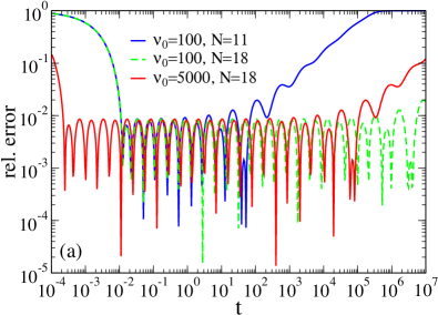
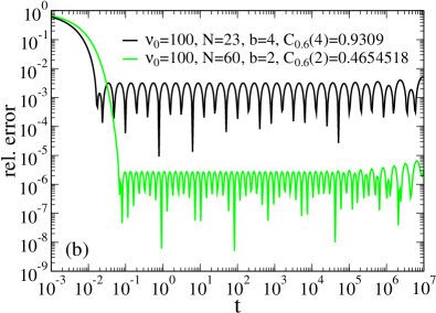
Figure 7: Relative error of the approximation (8) to a strict power-law dependence $1/t^{0.6}$ for $b=5,4,2$ and several different $N$ and $\nu_{0}$ shown in the plot. In part (a), $b=5$, $N=11$ and $N=18$. Part (b) shows that with lowering $b$ to $b=2$ and increasing $N$ to $N=60$ one can increase relative accuracy of approximation to better than $10^{-5}$ or 0.001%. It means that our embedding method can be made numerically exact in quite moderate embedding dimensions. Numerical accuracy of several per cents is, however, sufficient in most stochastic simulations.

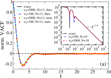
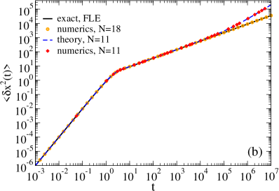
Figure 8: (a) Normalized velocity autocorrelation function (VACF) and (b) variance of the particle positions versus time for potential-free diffusion in the case $\alpha=0.6$. Exact analytical FLE results in Eqs. (2) and (3) are compared with the results of various quasi-analytical approximations and matching numerical results. Quasi-analytical results are obtained by a numerically precise inversion of the corresponding Laplace-transformed analytical results containing approximate memory kernels (8). Stochastic numerical results correspond to the same matching approximate kernels. They agree very well with quasi-analytical results for diffusion at all times, and also for VACF at sufficiently short times until statistical noise starts to dominate for small values of VACF. In the inset (a), the exact analytical result (2) is compared with two quasi-analytical approximations. Here, the absolute value of VACF is plotted.

For doing Markovian embedding, one introduces a set of $N$ viscoelastic forces $u_{i}$ such that the corresponding embedding dynamics in the hyperspace of dimension $D=N+2$ reads [64, 65]

$$\dot{x}(t) = v(t)$$

$$m\dot{v}(t) = f(x)+\sum^{N}_{i=1}u_{i}(t)$$

$$\dot{u}_{i}(t) = -k_{i}v(t)-\nu_{i}u_{i}(t)+\sqrt{2k_{B}Tk_{i}\nu_{i}}\zeta_{i}(t),$$ (9)

for $i=1,...,N$, where $\zeta_{i}(t)$, $i=1..N$, are $N$ delta-correlated in time and mutually uncorrelated white Gaussian noise sources of zero-mean and unit intensity, $\langle\zeta_{i}(t)\zeta_{j}(t^{\prime})\rangle=\delta_{ij}\delta(t-t^{\prime})$. The initial $u_{i}(0)$ are sampled as mutually independent Gaussian variables with zero mean and variances $\langle u_{i}^{2}(0)\rangle=k_{B}Tk_{i}$ [64, 65]. Eq. (A) corresponds to a Maxwell-Langevin model of stochastic viscoelastic dynamics developed in our previous work [64, 65] and used in numerous papers. The first two equations in Eq. (A) are just equations of motion expressing Newton’s second law. The last $N$ equations describe the relaxation of viscoelastic force modes of environment influenced by the particle motion. Such an equation corresponds to Maxwell’s idea that viscoelasticity can be described within a framework of an elastic force $u$ characterized by some elastic constant $k$, which can weaken in time and relax to zero with rate $\nu$ [129]. It is how Maxwell derived phenomenon viscosity from the phenomenon elasticity in his classical work [129] by course-graining over the times largely exceeding $1/\nu$. The last thermal noise term in Eq. (A) ensures that this viscoelastic force is consistent with thermodynamics and FDT [65], i.e., it models a thermal environment at local temperature $T$ and relaxes to equilibrium with rate $\nu$ for a localized particle, $v=0$. However, when a particle moves, it disturbs this local equilibrium, what creates a long-lasting memory in the environment for slowly relaxing modes $u_{i}$. These modes remember where the particle was before. Thereby, a slowly relaxing local deformation is created, which attracts and temporary traps the particle (viscoelastic caging). An analogy with polaron picture in solids is most useful here to grasp the physical mechanism of viscoelastic subdiffusion [64, 65]. Notice that this approach is straightforward to generalize [116, 117, 118] to include the effects of hydrodynamic memory [130, 131], and a normal friction component [65, 87]. The latter corresponds, e.g., the water content of cytosol. We do not consider them here.

Initially, particles were always prepared with their velocities Maxwell-distributed at temperature $T$ and localized sharply at some random, uniformly sampled in the spacial interval $[-L/2,L/2]$ positions $x_{i}(0)$. It is a non-equilibrium initial preparation. Particles are typically subjected to some local bias $f(x_{i}(0))$ and explore first some local environment. They can, e.g., be either trapped in some local potential minima or start at the tops of potential local hills, see in Fig. 1.

In numerical simulations, we use the second-order stochastic Heun algorithm [132] implemented in CUDA and run simulations on professional graphical processor units (GPUs) with double precision. In ensemble simulations, we run $M=10^{5}$ particles in parallel. With $\nu_{0}=100$, $\Delta t=0.005$ and $N=11$ viscoelastic modes, simulations require about 6.5 days to arrive at $t_{\rm max}=10^{7}$ on Titan V processors, and five times longer on older Kepler K20 GPUs. Embedding with $N=18$ on Titan V GPU requires about two weeks for the same integration time step. It sets the practical restrictions in simulations. We first test our approach on calculating VACF $K_{v}(t)$ and $\langle\delta x^{2}(t)\rangle$ in the potential-free case and comparing the results with exact result in equations (2), (3) for FLE dynamics. Results for normalized $K_{v}(t)$ are shown in Fig. 8 (a). For $\alpha=0.6$, $K_{v}(t)$ changes sign only once at $t_{1}\approx 1.76$ and remains negative for $t>t_{1}$. It is different, e.g., from the case $\alpha=0.5$, where the sign oscillations occur exactly three times [87]. At $t_{2}\approx 3.04$ it reaches first a minimum $K_{v}(t_{1})\approx-0.21286\,v_{T}^{2}$, and then increases and reaches a local maximum $K_{v}(t_{1})\approx-0.00275\,v_{T}^{2}$ at $t_{2}\approx 7.88$, not crossing zero. Then, it again decreases to a local minimum $K_{v}(t_{1})\approx-0.00984\,v_{T}^{2}$ at $t_{3}\approx 11.88$, and after this it gradually approaches zero in accordance with power-law $t^{-1.4}$. It has to be mentioned that such fine features are not detectable in stochastic numerical simulations using $M=10^{5}$ because of pure statistical relative error of the order $1/\sqrt{M}\approx 0.00316$ or 0.316%. Because of this reason, the numerical results in Fig. 8 (a) sink in the statistical errors already for $t>6$. Hence, a trustful comparison of stochastic numerical and (semi)-analytical results in part (a) can be made only for $t<6$. In part (b), however, the agreement between the exact and (semi)-analytical results, from one side, and numerical results, from another side, is nearly perfect for all times. To resolve the discussed fine features in part (a), we also plot (semi-)analytical results obtained by numerical inversion of the Laplace-transformed

$$\tilde{K}_{v}(s)=\frac{k_{B}T}{ms+\tilde{\eta}(s)}$$ (10)

with the Laplace-transformed memory kernel approximated by Laplace-transformed (8). In this case, $\tilde{K}_{v}(s)$ is a rational function of $s$, and it can be quasi-analytically inverted, while finding the roots of the corresponding polynomial of $s$ in denominator of this rational function numerically. However, for practical purposes it is best to use a Gaver-Stehfest series [133, 134] for the inversion of Laplace-transform with an adaptable (arbitrary in principle) numerical precision [135], as we did earlier in many papers, e.g., in [64]. This inversion of Laplace-transform allows us to arrive at numerically accurate results in many cases, including exact and approximate memory kernel in this paper. In the insert of Fig. 8 (a), where the exact (without cutoff) $|K_{v}(t)/v_{T}^{2}|$ and its two approximations are plotted on a doubly logarithmic scale, one can see that the approximation with $\nu_{0}=5000$ and $N=18$ excellently reproduces $K_{v}(t)$ on the whole time span depicted. The approximation with $\nu_{0}=100$ and $N=18$ also well reproduces all the features mentioned above. However, it makes some discrepancies from the exact FLE result near to the extrema of $K_{v}(t)$ in part (a) visible. Stochastic numerics in the main plot in Fig. 8 for $\nu_{0}=100$, $\nu_{0}=5000$ (done in this case with a much finer time-step $\Delta t=10^{-5}$), and $N=11$ also excellently agree with (semi)-analytical results obtained by numerical inversion of (10) [part (a)] and $2\tilde{K}_{v}(s)/s^{2}$ [part (b)]. The discussed small discrepancies in a small intermediate range of $t$ in part (a) does not influence the results already for $t>12$, where the overdamped FBM regime is established in the absence of external potential. For this reason, we used embedding with $\nu_{0}=100$, which allows for a much larger $\Delta t$ and makes feasible much large $t_{\rm max}$ in simulations. It is a typical trade-off between numerical accuracy and feasibility in numerical simulations. Moreover, we do not consider rigorously an FLE model in this paper, but rather a subdiffusive GLE model with memory cutoffs.

Appendix B Estimation of physical parameters

In this estimation, we have in mind some lipid systems, where inertial effects are clearly present in MD simulations on the initial time scale [30, 32]. For example, long-tail of VACF in MD simulations of a bilayer of 128 dioleoyl-sn-glycero-3-phosphocholine (DOPC) molecules at $T=310$ K, was fitted [30] with $\alpha=0.61$, $v_{T}^{2}=6.55\times 10^{-3}\;{\rm nm^{2}/ps^{2}}$, $\bar{D}_{\alpha}=0.101\;{\rm nm^{2}/ns^{\alpha}}$, yielding $v_{T}=0.0809\;{\rm nm/ps}$ and $\bar{\tau}_{v}=(\bar{D}_{\alpha}/v_{T}^{2})^{1/(1+\alpha)}=\tau_{v}/[\Gamma(1+\alpha)]^{1/(2-\alpha)}=0.35$ ps or $\tau_{v}=0.323$ ps. Then, $x_{0}=v_{T}\tau_{v}\approx 0.026$ nm or 0.26 Å. In these units, $\lambda=10$ would correspond to 2.6 Å, and $\lambda=100$ to 2.6 nm. The maximal time $t_{\rm max}=10^{7}$ in our simulations would correspond to 3.23 $\mu s$. Notice, however, that they are done not for a particular lipid or lipid/protein system, but present results of a generic physical model, and we are just playing with parameters. They serve merely for readers’ orientation. We use $\alpha=0.6$ in simulations.

References

- [1] Mason T G and Weitz D A 1995 Phys. Rev. Lett. 74 1250–1253
- [2] Amblard F, Maggs A C, Yurke B, Pargellis A N and Leibler S 1996 Phys. Rev. Lett. 77 4470–4473
- [3] Wong I Y, Gardel M L, Reichman D R, Weeks E R, Valentine M T, Bausch A R and Weitz D A 2004 Phys. Rev. Lett. 92 178101
- [4] Waigh T A 2005 Rep. Progr. Phys. 68 685
- [5] Santamaria-Holek I, Rubi J M and Gadomski A 2007 J. Phys. Chem. B 111 2293–2298
- [6] Weiss M 2013 Phys. Rev. E 88 010101
- [7] Evers F, Hanes R D L, Zunke C, Capellmann R F, Bewerunge J, Dalle-Ferrier C, Jenkins M C, Ladadwa I, Heuer A, Castaneda-Priego R and Egelhaaf S U 2013 Eur. Phys. J. Spec. Top. 222 2995
- [8] Hanes R D L, Dalle-Ferrier C, Schmiedeberg M, Jenkins M C and Egelhaaf S U 2012 Soft Matter 8 2714–2723
- [9] Hanes R D L, Schmiedeberg M and Egelhaaf S U 2013 Phys. Rev. E 88 062133
- [10] Saxton M J and Jacobsen K 1997 Ann. Rev. Biophys. Biomolec. Struc. 26 373–399
- [11] Weiss M, Elsner M, Kartberg F and Nilsson T 2004 Biophys. J. 87 3518–3524
- [12] Tolic-Norrelykke I M, Munteanu E L, Thon G, Oddershede L and Berg-Sorensen K 2004 Phys. Rev. Lett. 93 078102
- [13] Banks D S and Fradin C 2005 Biophys. J. 89 2960–2971
- [14] Golding I and Cox E C 2006 Phys. Rev. Lett. 96 098102
- [15] Guigas G, Kalla C and Weiss M 2007 Biophys. J. 93 316
- [16] Szymanski J and Weiss M 2009 Phys. Rev. Lett. 103 038102
- [17] Weigel A V, Simon B, Tamkun M M and Krapf D 2011 Proc. Natl. Acad. Sci. (USA) 108 6438–6443
- [18] Höfling F and Franosch T 2013 Rep. Prog. Phys. 76 046602
- [19] Jeon J H, Tejedor V, Burov S, Barkai E, Selhuber-Unkel C, Berg-Sørensen K, Oddershede L and Metzler R 2011 Phys. Rev. Lett. 106 048103
- [20] Luby-Phelps K 2013 Mol. Biol. Cell 24 2593
- [21] Pan W, Filobelo L, Pham N D Q, Galkin O, Uzunova V V and Vekilov P G 2009 Phys. Rev. Lett. 102 058101
- [22] Harrison A W, Kenwright D A, Waigh T A, Woodman P G and Allan V J 2013 Phys. Biol. 10 036002
- [23] Parry B R, Surovtsev I V, Cabeen M T, O’Hern C S, Dufresne E R and Jacobs-Wagner C 2014 Cell 156 183
- [24] Robert D, Nguyen T H, Gallet F and Wilhelm C 2010 PLoS ONE 4 e10046
- [25] Bertseva E, Grebenkov D, Schmidhauser P, Gribkova S, Jeney S and Forro L 2012 Eur. Phys. J. E 35 63
- [26] Regner B, Vucinic D, Domnisoru C, Bartol T, Hetzer M, Tartakovsky D and Sejnowski T 2013 Biophys. J. 104 1652 – 1660
- [27] Manzo C, Torreno-Pina J A, Massignan P, Lapeyre G J, Lewenstein M and Garcia Parajo M F 2015 Phys. Rev. X 5 011021
- [28] Lampo T J, Stylianidou S, Backlund M P, Wiggins P A and Spakowitz A J 2017 Biophys. J. 112 532 – 542
- [29] Schwille P, Haupts U, Maiti S and Webb W W 1999 Biophys. J 77 2251
- [30] Kneller G R, Baczynski K and Pasenkiewicz-Gierula M 2011 J. Chem. Phys. 135 141105
- [31] Sezgin E, Levental I, Grzybek M, Schwarzmann G, Mueller V, Honigmann A, Belov V N, Eggeling C, Coskun U, Simons K and Schwille P 2012 Biochem. Biophys. Acta (BBA) - Biomembr. 1818 1777 – 1784
- [32] Jeon J H, Monne H M S, Javanainen M and Metzler R 2012 Phys. Rev. Lett. 109 188103
- [33] Jeon J H, Javanainen M, Martinez-Seara H, Metzler R and Vattulainen I 2016 Phys. Rev. X 6 021006
- [34] Metzler R, Jeon J H and Cherstvy A G 2016 Biochem. Biophys. Acta 1858 2451
- [35] Wang Y M, Austin R H and Cox E C 2006 Phys. Rev. Lett. 97 048302
- [36] Goychuk I and Kharchenko V O 2014 Phys. Rev. Lett. 113 100601
- [37] Kong M, Liu L, Chen X, Driscoll K I, Mao P, Böhm S, Kad N M, Watkins S C, Bernstein K A, Wyrick J J, Min J H and Houten B V 2016 Mol. Cel. 64 376–387
- [38] Kong M and Houten B V 2017 Prog.Biophys. Mol. Biolog. 127 93–104
- [39] Liu L, Kong M, Gassman N R, Freudentha B D, Prasad R, Zhen S, Watkins S C, Wilson S H and Houten B V 2017 Nucl. Acid. Res. 45 12834–12847
- [40] Yang H, Luo G, Karnchanaphanurach P, Louie T M, Rech I, Cova S, Xun L and Xie X S 2003 Science 302 262–266
- [41] Goychuk I and Hänggi P 2004 Phys. Rev. E 70 051915
- [42] Kneller G R and Hinsen K 2004 J. Chem. Phys. 121 10278
- [43] Kou S C and Xie X S 2004 Phys. Rev. Lett. 93 180603
- [44] Min W, Luo G, Cherayil B J, Kou S C and Xie X S 2005 Phys. Rev. Lett. 94 198302
- [45] Calandrini V, Abergel D and Kneller G R 2010 J. Chem. Phys. 133 145101
- [46] Calligari P A, Calandrini V, Kneller G R and Abergel D 2011 J. Phys. Chem. B 115 12370–12379
- [47] Calligari P A, Calandrini V, Ollivier J, Artero J B, Härtlein M, Johnson M and Kneller G R 2015 J. Phys. Chem. B 119 7860–7873
- [48] Goychuk I 2015 Phys. Rev. E 92 042711
- [49] Hu X, Hong L, Smith M D, Neusius T, Cheng X and Smith J C 2016 Nat. Phys. 12 171–174
- [50] Shlesinger M F 1974 J. Stat. Phys. 10 421–434
- [51] Scher H and Montroll E W 1975 Phys. Rev. B 12 2455–2477
- [52] Hughes B D 1995 Random Walks and Random Environments (Oxford: Clarendon Press)
- [53] ben Avraham D and Havlin S 2000 Diffusion and Reactions in Fractals and Disordered Systems (Cambridge: Cambridge University Press)
- [54] Metzler R and Klafter J 2000 Phys. Rep. 339 1 – 77
- [55] Metzler R, Jeon J H, Cherstvy A G and Barkai E 2014 Phys. Chem. Chem. Phys. 16 24128–24164
- [56] Barkai E, Garini Y and Metzler R 2012 Phys. Today 65 (8) 29
- [57] He Y, Burov S, Metzler R and Barkai E 2008 Phys. Rev. Lett. 101 058101
- [58] Goychuk I and Hänggi P 2003 Phys. Rev. Lett. 91 070601
- [59] Goychuk I 2012 Phys. Rev. E 86 021113
- [60] Goychuk I 2014 Comm. Theor. Phys. 62 497
- [61] Metzler R, Barkai E and Klafter J 1999 Phys. Rev. Lett. 82 3563–3567
- [62] Goychuk I, Heinsalu E, Patriarca M, Schmid G and Hänggi P 2006 Phys. Rev. E 73 020101 (R)
- [63] Goychuk I 2007 Phys. Rev. E 76 040102 (R)
- [64] Goychuk I 2009 Phys. Rev. E 80 046125
- [65] Goychuk I 2012 Adv. Chem. Phys. 150 187–253
- [66] Goychuk I 2012 Fluct. Noise Lett. 11 1240009
- [67] Goychuk I and Hänggi P 2007 Phys. Rev. Lett. 99 200601
- [68] Goychuk I 2019 Phys. Rev. Lett. 123 238902
- [69] Goychuk I 2019 Phys. Rev. E 99 052136
- [70] Kubo R 1966 Rep. Prog. Theor. Phys. 29 255
- [71] Zwanzig R 1973 J. Stat. Phys. 9 215–220
- [72] Kubo R, Toda M and Hashitsume M 1985 Statistical Physics II, Nonequilibrium Statistical Mechanics (Berlin: Springer)
- [73] Zwanzig R 2001 Nonequilibrium Statistical Mechanics (Oxford: Oxford University Press)
- [74] Mainardi F and Pironi P 1996 Extracta Math. 11 140–154
- [75] Lutz E 2001 Phys. Rev. E 64 051106
- [76] Kolmogorov A N 1940 Dokl. Akad. Nauk SSSR 26 115–118 (in Russian)
- [77] Kolmogorov A N 1991 Wiener spirals and some other interesting curves in a hilbert space Selected Works of A. N. Kolmogorov, vol. I, Mechanics and Mathematics ed Tikhomirov V M (Dordrecht: Kluwer) pp 303–307
- [78] Mandelbrot B and van Ness J 1968 SIAM Rev. 10 422
- [79] Romero A H and Sancho J M 1998 Phys. Rev. E 58 2833–2837
- [80] Khoury M, Lacasta A M, Sancho J M and Lindenberg K 2011 Phys. Rev. Lett. 106 090602
- [81] Lindenberg K, Sancho J M, Khoury M and Lacasta A M 2012 Fluct. Noise Lett. 11 1240004
- [82] Simon M S, Sancho J M and Lindenberg K 2013 Phys. Rev. E 88 062105
- [83] Goychuk I, Kharchenko V O and Metzler R 2017 Phys. Rev. E 96 052134
- [84] Massignan P, Manzo C, Torreno-Pina J A, García-Parajo M F, Lewenstein M and Lapeyre G J 2014 Phys. Rev. Lett. 112 150603
- [85] Magdziarz M, Weron A, Burnecki K and Klafter J 2009 Phys. Rev. Lett. 103 180602
- [86] Tabei S M A, Burov S, Kima H Y, Kuznetsov A, Huynha T, Jureller J, Philipson L H, Dinner A R and Scherer N F 2013 Proc. Natl. Acad. Sci. (USA) 110 4911–4916
- [87] Goychuk I 2018 Phys. Chem. Chem. Phys. 20 24140–24155
- [88] Caspi A, Granek R and Elbaum M 2002 Phys. Rev. E 66 011916
- [89] Weber S C, Spakowitz A J and Theriot J A 2010 Phys. Rev. Lett. 104 238102
- [90] Bruno L, Salierno M, Wetzler D E, Desposito M A and Levi V 2011 PLoS ONE 6 e18332
- [91] Lubelski A, Sokolov I M and Klafter J 2008 Phys. Rev. Lett. 100 250602
- [92] Deng W and Barkai E 2009 Phys. Rev. E 79 011112
- [93] Bouchaud J P and Georges A 1990 Phys. Rep. 195 127 – 293
- [94] Sinai Y G 1982 Theor. Prob. Appl. 27 247 – 258
- [95] Bouchaud J, Comtet A, Georges A and Doussal P L 1990 Ann. Phys. (N.Y.) 201 285–341
- [96] Le Doussal P, Monthus C and Fisher D S 1999 Phys. Rev. E 59 4795–4840
- [97] Bässler H 1993 Phys. Stat. Solidi B 175 15–56
- [98] Dunlap D H, Parris P E and Kenkre V M 1996 Phys. Rev. Lett. 77 542–545
- [99] Bässler H 1987 Phys. Rev. Lett. 58 767–770
- [100] Hecksher T, Nielsen A I, Olsen N B and Dyre J C 2008 Nat. Phys. 4 737–741
- [101] Gerland U, Moroz J D and Hwa T 2002 Proc. Natl. Acad. Sci. (USA) 99 12015–12020
- [102] Slutsky M, Kardar M and Mirny L A 2004 Phys. Rev. E 69 061903
- [103] Lässig M 2007 BMC Bioinformatics 8(Suppl. 6) S7
- [104] Bénichou O, Kafri Y, Sheinman M and Voituriez R 2009 Phys. Rev. Lett. 103 138102
- [105] Sheinman M, Bénichou O, Kafri Y and Voituriez R 2012 Rep. Progr. Phys. 75 026601
- [106] Gennes P G D 1975 J. Stat. Phys. 12 463–481
- [107] Hänggi P, Talkner P and Borkovec M 1990 Rev. Mod. Phys. 62 251–341
- [108] Hanes R D L and Egelhaaf S U 2012 J. Phys.: Cond. Matt. 24 464116
- [109] Elf J, Li G W and Xie X S 2007 Science 316 1191–1194
- [110] Duan H G and Liang X T 2012 Eur. Phys. J. B 85 209
- [111] Javanainen M, Hammaren H, Monticelli L, Jeon J H, Miettinen M S, Martinez-Seara H, Metzler R and Vattulainen I 2013 Faraday Discuss. 161 397–417
- [112] Bogolyubov N N 1945 On some Statistical Methods in Mathematical Physics (Kiev: Ukrainian Academy of Sciences) (in Russian)
- [113] Ford G W, Kac M and Mazur P 1965 J. Math. Phys. 6 504
- [114] Weiss U 1999 Quantum Dissipative Systems 2nd ed (Singapore: World Scientific)
- [115] Simon M S, Sancho J M and Lacasta A M 2012 Fluct. Noise Lett. 11 1250026
- [116] Siegle P, Goychuk I and Hänggi P 2011 EPL 93 20002
- [117] Goychuk I 2019 Phys. Rev. Lett. 123 180603
- [118] Goychuk I and Pöschel T 2020 Phys. Rev. E 102 012139
- [119] Papoulis A 1991 Probability, Random Variables, and Stochastic Processes 3rd ed (New York: McGraw-Hill Book Company)
- [120] Yaglom A M 1972 An Introduction to the Theory of Stationary Random Functions (New York: Dover Publications)
- [121] Goychuk I 2017 Phys. Chem. Chem. Phys. 19 3056
- [122] Prony R 1795 J. Ecole Polytech. 1 24–76
- [123] Hauer J F, Demeure C J and Scharf L L 1990 IEEE Trans. Power Syst. 5 80–89
- [124] Park S W and Schapery R A 1999 Int. J. Solids Struct. 36 1653 – 1675
- [125] Schapery R A and Park S W 1999 Int. J. Solids Struct. 36 1677 – 1699
- [126] Palmer R G, Stein D L, Abrahams E and Anderson P W 1984 Phys. Rev. Lett. 53 958–961
- [127] Bochud T and Challet D 2007 Quant. Finance 7 585–589
- [128] McKinley S A, Yao K and Forest M G 2009 J. Rheol. 53 1489
- [129] Maxwell J C 1867 Phil. Trans. R. Soc. Lond. 157 49–88
- [130] Franosch T, Grimm M, Belushkin M, Mor F M, Foffi G, Forro L and Jeney S 2011 Nature (London) 478 85–88
- [131] Huang R, Chavez I, Taute K M, Lukic B, Jeney S, Raizen M G and Florin E L 2011 Nat. Phys. 7 576–580
- [132] Gard T C 1988 Introduction to Stochastic Differential Equations (New York: Dekker)
- [133] Stehfest H 1970 Commun. ACM 13 47–49
- [134] Stehfest H 1970 Commun. ACM 13 624 (Erratum)
- [135] Valkó P P and Vajda S 2002 Inverse Probl. Engin. 10 467–483