Investing with Cryptocurrencies – evaluating their potential for portfolio allocation strategies

Abstract

Abstract

Cryptocurrencies (CCs) have risen rapidly in market capitalization over the last years. Despite striking price volatility, their high average returns have drawn attention to CCs as alternative investment assets for portfolio and risk management. We investigate the utility gains for different types of investors when they consider cryptocurrencies as an addition to their portfolio of traditional assets. We consider risk-averse, return-seeking as well as diversification-preferring investors who trade along different allocation frequencies, namely daily, weekly or monthly. Out-of-sample performance and diversification benefits are studied for the most popular portfolio-construction rules, including mean-variance optimization, risk-parity, and maximum-diversification strategies, as well as combined strategies. To account for low liquidity in CC markets, we incorporate liquidity constraints via the LIBRO method. Our results show that CCs can improve the risk-return profile of portfolios. In particular, a maximum-diversification strategy (maximizing the Portfolio Diversification Index, PDI) draws appreciably on CCs, and spanning tests clearly indicate that CC returns are non-redundant additions to the investment universe. Though our analysis also shows that illiquidity of CCs potentially reverses the results.

Keywords: cryptocurrency, CRIX, investments, portfolio management, asset classes, blockchain, Bitcoin, altcoins, DLT

JEL Classification: C01, C58, G11

1 Introduction

Cryptocurrencies (CCs) have exhibited remarkable performance in the decade since [(81)] invented the blockchain. Accompanied by huge inflows of capital into the market and strong swings in prices, CCs have gained strongly in market value. Accordingly, indices like CRIX [(108), thecrix.de] were introduced to capture the market evolution and provide a basis for ETFs. Driven by these developments, cryptocurrency markets became increasingly attractive to investors, who have started to consider CCs as a novel class of alternative investments. However, investors differ with regard to their risk profiles, investment targets, individual trading behaviors, and generally their diverse motives and preferences, and thus the perspective to include CCs into financial portfolios raises a number of questions:

1. For whom is investing in the CC market valuable? Is the benefit derived from adding CCs to a portfolio dependent on the investor’s objectives (e.g., return-oriented or diversification seeking)?

2. To which type of investor are CC investments most useful? Only professional traders who rebalance their portfolio frequently, or also less actively trading retail investors?

3. Should investors focus on one particular coin (e.g., Bitcoin), a selected few, or rather build a portfolio of a broad selection of CCs?

When an investor does decide to include CCs in the portfolio, further questions arise about the choice of CCs for investment and their portfolio weights:

1. What exposure to each CC should be held in the portfolio? How informative are past prices, how stable are positions when re-balancing the portfolio? Do model-free strategies like equal-weighting provide reasonable results?

2. Can these strategies be implemented in practice? In particular, are all CCs liquid enough for inclusion in an investment portfolio? If not, how can investors still profit from promising CCs with little trading volume without exposing their portfolio too much to illiquidity? Moreover, how is performance affected by honoring such portfolio restrictions?

3. Overall, how do the properties of CC returns affect portfolios? Is a certain type of portfolio-allocation method more suitable to manage and simultaneously exploit their properties?

While we review the literature extensively in Section 2, clearly numerous studies have investigated the properties referred to in Question 6, and agree that CCs exhibit remarkably high average realized returns by the standards of traditional financial assets—and correspondingly high risk and uncertainty. Not only is price volatility high; also unfavorable properties obtrude, including frequent pricing bubbles [(45), (49), (23), (83)], accumulation of jumps [(96)], even evidence of price manipulation [(46)].

At the same time, there is evidence of low correlations of CC returns with those of traditional financial assets and other CCs. Therefore, the high risk of CC positions may be compensated by appropriate returns as well as provide an opportunity to increase portfolio diversification. Results to that effect have been spearheaded by [(18), (37)], the first to include Bitcoin (BTC) in a portfolio of traditional assets, and subsequently bolstered by [(39)], who include a broad cross-section of CCs, [(30)], who instead add CRIX, and lately [(87), (5)], who include Bitcoin in advanced portfolio optimization and find it enhances the risk-return profile.

So evidence exists that CCs can be beneficial for investors [(85)]. However, taking the investor’s perspective, we see that while prior studies have covered crucially important aspects of investing with CCs, the outlined questions 1–5 remain fundamentally unanswered, for at least two reasons. First, the key result of a diversification benefit of CCs (or BTC) cannot be established unless a broad set of non-CC alternative investments are included. For simplicity, in this paper we refer to all non-CC investments as “traditional assets,” including alternative investments like gold or real estate, in order to focus on the potential of adding CCs to well-diversified portfolios. Second, it remains unclear which strategies can actually be implemented in practice unless specific care is taken to address the frequently extremely dry liquidity in CC markets.

The importance of addressing liquidity concerns is pinpointed by [(109)], who introduce LIquidity Bounded Risk-return Optimization (LIBRO) when considering a large sample of CCs added to a portfolio consisting of the S&P100, US bonds and commodities. Given the low liquidity of CCs as compared to traditional markets, LIBRO is designed to protect investors from an inability to trade a CC in necessary amounts due to low trading volume.

Against this background, we address the questions above by performing a large-scale comparative investment-strategy study including both a broad range of traditional assets together with a broad cross-section of CCs. Therein, we test the performance of an extensive set of common investment strategies and thus consider different types of investors, while we employ the LIBRO method to handle liquidity concerns. We consider risk-oriented, return-oriented, risk-return-oriented, and combined strategies; see Table 1 for a full list of strategies under consideration. We estimate extending-window and rolling-window approaches optimizations for a sizable breadth of different common objective functions. Finally, we compare all strategies based on three different re-allocation frequencies, namely daily, weekly and monthly, providing results for investors trading at different frequencies. To the best of our knowledge, we thus present the broadest study on investing with CCs conducted so far.

Closest related to our paper are [(5)] and [(87)], both also studying the influence of CC investment on optimal portfolio composition. However, both include only Bitcoin, whereas we consider a broad cross-section of 52 distinct CC price series. Moreover, both consider fewer traditional assets: industry portfolios (so equity only) in the former paper, US equity and bond investments in the latter, plus commodities in a robustness test. In contrast, our set of traditional assets is critically broader: first, as CCs trade globally, our international approach includes equity returns for each of the 5 major economic areas (Europe, USA, Japan, UK, China), as well as region-specific bond returns. Second, we always include alternative investments, namely gold, real estate, commodities, and the returns to FX trades between the five regions’ fiat currencies. Table 2 lists the traditional assets all our portfolios include. As we have pointed out, this emphatically goes beyond quantitatively extending prior studies: unless both a broad cross-section of CCs and of traditional assets are included, it remains impossible to determine the magnitude of diversification benefits, and more critically, also impossible to distinguish whether apparent benefits of CCs are indeed present, or if CCs merely proxy for alternative assets.

Moreover, we cover a longer time horizon, and can thus include more than 2 years after peak CC prices; also, we consider more allocation strategies. Most importantly, since we take the investor’s perspective, we implement LIBRO and contrast portfolios with weights that observe the liquidity constraints with otherwise identical portfolios which do not: it turns out to cricitally affect performance for several popular trading strategies.

Our study contributes to answering questions 1–6. Spanning tests show that more than $50\%$ of the CCs considered can improve the efficient frontier of a portfolio containing even our broad set of traditional assets. We show that purely risk-minimizing investors will optimally choose to mostly forego CC investment; however, for investors with higher target returns their addition seriously expands the efficient frontier. Diversification-oriented investors benefit most, even in terms of maximizing cumulative wealth. We also document that a lower rebalancing frequency (monthly) of the portfolios generally enhances cumulated returns. As mentioned, we confirm that several CCs exhibit low liquidity, which can be tackled with the LIBRO approach. Our results highlight the severity of low-liquidity risk, and how analyses that do not take this risk into account will compute investment returns that are infeasible for any but the smallest personal portfolios.

The paper is organized as follows. First, Section 2 reviews the related literature. Section 3 provides an overview of the asset-allocation models under consideration, with a focus on connections between them; therein Section 3.2 explains the approach of model averaging across investment strategies. Section 4 reviews the LIBRO method. In Section 5 we explain the methodology for comparing the performance of the models considered. Our dataset of portfolio components is described in Section 6, and Section 7 presents the results of our analyses of out-of-sample performance of all portfolio strategies with CCs and traditional assets. We conclude in Section 8.

Code to produce the results of this paper is available via www.quantlet.de missing.

2 Literature review

Modern portfolio theory builds on the CAPM [(74), (103), (69)], both a theoretical equilibrium model and a directly applicable statistical approach. Yet, financial markets do not meet its assumptions, so it lacks empirical accuracy. Asset pricing and portfolio optimization address this lack in one of two ways.

The first we call the financial-economics approach: it follows [(94)]’s (94) arbitrage-pricing theory which keeps the linear structure and adds more factors to capture systematic patterns in returns. Popularized by Fama_French_1992 (42, 40), it was extended to factors for momentum (Jegadeesh_Titman_1993, 58, 21) or profitability and investment (Fama_French_2015, 41). In principle, the approach renders portfolio optimization straightforward and unidimensional: a portfolio is better, the higher its alpha (the intercept after accounting for all factors’ loadings). In practice, the choice of factors depends on the investment universe, and also for given asset classes controversy remains about factors (the “zoo” of Cochrane_2011, 33), how to choose them (Feng_Giglio_Xiu_2020, 43), even basic methodology (NovyMarx_2014, 82).

A strand of the literature on cryptocurrencies (CCs) is devoted to finding and using factors in CC markets (see Liu_Tsyvinski_2019, 72, 38, 56, 106, 104); however, in this paper we pursue the second approach.

We term it the quantitative-finance approach, due to its statistical nature. Its idea, in essence, says: if we can capture the (joint) return distribution (and its dynamics) of all investable assets (and parameters affecting them), then we can directly estimate portfolio weights to optimize the desired performance metric. Owing to the abundance of statistical techniques for the variety of modelling choices and investment objectives, this approach is most common in fund management. However, the easy customization has precluded a standard, unique approach. A portfolio’s optimal allocation thus depends crucially on three elements: the investment universe, the investment strategy, and the investment objective as defined by the metric of optimization.

Most fundamental is the determination of the investment universe. Our paper focuses on its role by analyzing it for extensive sets of common strategies and objective functions; concretely, on the potential of adding CCs. Historically, starting from stocks and a risk-free interest rate, the diversification benefits to adding bonds (Liu_2016, 70), foreign exchange (Kroencke_Schindler_Schrimpf_2013, 66, 9, 2), real estate (Benjamin_Sirmans_Zietz_2001, 12, 3), and commodities (Belousova_Dorfleitner_2012, 11) including gold (Hoang_et_al_2015, 52) have been established in the literature. We term all these assets “traditional investments”, and we include proxies for all of them in our benchmark portfolio. This breadth is key, as our goal is to investigate the effect of including additionally CCs. Only the broad traditional portfolio ensures we assess the diversification potential of CCs as investments: otherwise, CCs might merely substitute for other alternative investments.

Considering CCs as investments contains subtle irony, as Nakamoto_2008 (81) pseudonymously introduced the blockchain as a technology to serve as money, not a profitable investment opportunity. Thus, initially doubt and debate shrouded the economic role of CCs (Glaser_et_al_2014, 47, 115, 14, 10).

However, after more than a decade of increasing demand, market capitalizations, and trading volumes for a multiplying number of CCs, the recently flourishing academic literature converges to the consensus that CCs constitute investments, generally, and a distinct asset class in particular. This literature can be categorized along two dimensions: first, which CC investment is considered? Only Bitcoin, also a fistful of other highly visible CCs like Ethereum or Ripple, or a broad cross-section of tradable CCs? Second, which portfolio allocations are considered? Only the CC(s), or also traditional markets? If the latter, only equity markets, or a broad range of traditional investments?

Regarding the first point, the literature started by investigating the properties of the Bitcoin price process (Kristoufek_2015, 65, 28, 22, 110, 13, 8, 84, 71), establishing, in essence, the presence of all critical properties of equity returns, yet often up to an order of magnitude stronger: CCs exhibit exceptionally high mean returns, and likewise volatility and drawdowns; returns also feature extremely heavy tails and high heteroskedasticity. Correlations with common return series turn out extremely low to non-existent.

Given such low correlations, it is intuitive why including Bitcoin can enhance a portfolio of traditional assets. Whereas the high riskiness leads to low portfolio weights for risk-averse investors, an inclusion is beneficial as it improves diversification.

At the same time, exploding interest in blockchain led to an explosion in the number of investable CCs. This kickstarted investigations into the joint-return properties of a broad cross-section of CCs (elendner_cross-section_2017, 39, 112, 16, 116, 113), which confirmed the return characteristics of Bitcoin to be representative for the entire asset class; yet generally so-called altcoins exhibit still higher risk and mean returns. (Even more extreme were returns of Initial Coin Offerings, ICOs, in particular during their peak in 2017—see, for instance, Adhami_Guidici_Martinazzi_2018 (4, 78, 80, 79). However, despite the important economic role of ICOs and STOs (Security Token Offerings) as novel channels of venture-capital investment, they are unsuitable for rules-based portfolio allocation, and hence fall outside the scope of our paper.)

A key finding is that correlations are low even among CCs, as long as they are no close substitutes or forks. This implies a potential diversification benefit from a broad basket of CCs (chuen2017cryptocurrency, 30). Alessandretti2018 (6), optimizing CCs-only portfolios with LSTMs and decision trees, also find enhanced return performance.

As one consequence, CC indices were developed: The CRIX (trimborn_crix_2016, 108) captures the broad CC market movement with a statistically optimized varying number of constituents; CCI30 (rivin2018cci30, 91) is a simple, close analogue to stock-market indices; F5 (Elendner_2018, 38) is a momentum-factor-based, transaction-cost-optimised basis for an exchange-traded portfolio; C20 (crypto20, 101) is an on-chain crypto-asset itself. VCRIX (Kim2019, 63) is a volatility index for option pricing. A first paper on option pricing of cryptos is Hou_et_al_2020 (53).

The second key finding of cross-sectional analyses is that CCs beyond the most prominent exhibit considerably low liquidity. Portfolio calculations ignoring liquidity might suggest trades which are impossible without extreme price impact. trimborn_investing_2017 (109) introduce LIquidity Bounded Risk-return Optimization (LIBRO) to account for illiquidity in CC portfolio formation. Since our focus is to evaluate the potential of adding CCs to traditional portfolios, i.e., we take the investor’s perspective, we provide results both without and with the inclusion of LIBRO constraints.

In summary, the literature on CCs so far has solidly established potential benefits of holding CCs in investment portfolios (foremost high returns and low correlations), as well as certain difficulties (critically low liquidity). Yet open questions remain; prime among those whether CCs “only” proxy for alternative (non-CC) assets, or provide investment opportunities that cannot be realized without CC positions. We close this gap by evaluating a wide range of common asset-allocation models with and without CC positions.

3 Asset-allocation models

Consider a matrix $X\in\mathbb{R}^{P\times N}$ of log returns of $N$ assets for $P$ days. In our comparative analysis we rely on a moving-window approach. Specifically, we choose an estimation window of length $K=252$ days (corresponding to the number of trading days in a calendar year). We investigate the performance of strategies for three rebalancing frequencies $k$: monthly, with $k=21$ days, weekly, with $k=5$ days, and daily with $k=1$ day. For each rebalancing period $t$ ($t=1,\dots,T$, with $T$ the number of moving windows, defined as $T=\frac{P-K}{k}$), starting on date $K+1$, we use the data in the previous $K$ days to estimate the parameters required to implement a particular strategy. These parameter estimates are then used to determine the relative portfolio weights $w$ in the portfolio of risky assets. Based on these weights, we compute the strategy’s return in rebalancing period $t+1$. This process is iterated by adding the $k$ daily returns for the next period in the dataset and dropping the corresponding earliest returns, until the end of the dataset is reached. The outcome of this rolling-window approach is a series of $P-K$ daily out-of-sample returns generated by each of the portfolio strategies listed in Table 1. To simplify notation, we omit the index $t$ for moving window or rebalancing period.

The traditional evaluation literature (e.g., demiguel2009optimal, 34, 97) considers an investor whose preferences are specified in terms of utility functions and fully described by the portfolio mean $\mu_{P}$ and variance $\sigma_{P}$. However, merton1980estimating (77) showed that a very long time series is required in order to receive accurate estimates of expected returns. Due to this high margin of error of expected-return estimates some authors, including haugen1991efficient (51), chopra1993effect (24) and chow2011survey (27), suggest to rely only on estimates of the covariance matrix as input of the optimization procedure. Thus, investors assume that all stocks have the same expected returns and under this strong assumption the optimal portfolio is the global minimum-variance portfolio. The minimum-variance portfolio strategy represents one of the so-called risk-based portfolios, i.e., the only input used is the estimate of the variance-covariance matrix. In this paper we consider the most popular ones: Maximum Diversification, Risk-Parity, Minimum Variance and Minimum CVaR portfolio. In Section 3.1 we describe the individual strategies from the portfolio-choice literature that we consider. In addition totraditional approaches, we consider a decision maker with risk preferences specified in percentile terms, and portfolio construction based on higher moments of the portfolio return-distribution, such as skewness and kurtosis. Therefore, in our comparative study we distinguish three groups of strategies: return-oriented, risk-oriented (or risk-based, as in clarke2013risk (31)), as well as a tangency portfolio with Maximum Sharpe Ratio (MV-S), which we categorize as a risk-return-oriented strategy.

Taking into account that the ranking of models changes over time, and motivated by the fact that in many fields a combination of models performs well (see, e.g., clemen1989combining, 32, 7), we also extend our analysis to include the combination of portfolio models based on a bootstrap approach inspired by schanbacher2014combining (97, 98). The detailed methodology of combined portfolio models is discussed in Section 3.2.

3.1 Common asset-allocation models

In this section we review those models that we consider in the empirical analysis. We also discuss links between the strategies and give conditions under which they are equivalent. In general, when bringing the theoretical models to the data, we employ in-sample moments of return distributions as estimators of their theoretical counterparts; naturally, all evaluation then concerns out-of-sample performance. As subsequent prices provide new information about assets’ returns, all estimates are updated before any rebalancing trades.

In all models we rule out short selling, a standard assumption in the CC literature, given that—with the exception of bitcoin, for which futures are traded since December 2017—taking short positions on CCs is at the very least impractical, if not outright impossible.

3.1.1 Equally-weighted portfolio

The most naïve portfolio strategy sets equal weights (EW) for all constituents: every asset gets a weight $w_{i}=1/N$ for $i=1,\dots,N$. If all constituents have the same expected returns and covariances, the EW portfolio is mean-variance optimal. However, there is no need for assumptions or estimates regarding the distribution of the assets’ returns to implement EW. Moreover, as demiguel2009optimal (34) show, EW allocations can actually perform well, in particular in settings of high uncertainty, i.e., parameter instability—the model-free approach avoids overfitting. This is also the reason why the F5 crpto strategy builds on an EW baseline benchmark.

3.1.2 Optimal mean-variance portfolio

Many portfolio managers still rely on Markowitz’ risk-return or mean-variance (MV) rule, combining assets into an efficient portfolio offering a risk-adjusted target return (hardle_applications_2015, 50). MV portfolios are optimal if the financial returns follow a normal distribution (which, generally, they do not), or if risk can be fully captured via volatility (which, generally, it cannot). Otherwise, MV serves as an approximation, which in favor of tractability and convenience accepts the drawbacks widely discussed in the literature: high portfolio concentration, i.e., high portfolio weights for a limited subset of the investment universe, and high sensitivity to small changes in parameter estimates of $\mu$ and $\sigma$, see jorion1985international (60), simaan1997estimation (105), kan2007optimal (62). In a Gaussian world, portfolio weights $w$ are obtained by solving the following optimization problem:

$$\underset{w\in\mathbb{R}^{p}}{\text{min}} \sigma_{P}^{2}(w)\stackrel{{\scriptstyle\operatorname{def}}}{{=}}w^{\top}\Sigma w$$ (1)

    s.t. $$\mu_{P}(w)=r_{T},$$

$$w^{\top}1_{N}=1,\hskip 8.53581ptw_{i}\geq 0$$

where $\Sigma\stackrel{{\scriptstyle\operatorname{def}}}{{=}}{{\operatorname{\text{E}}}}_{t-1}\{(X-\mu)(X-\mu)^{\top}\}$ and $\mu\stackrel{{\scriptstyle\operatorname{def}}}{{=}}{{\operatorname{\text{E}}}}_{t-1}(X)$ are the sample covariance matrix and vector of mean returns respctively, $\mu_{P}(w)\stackrel{{\scriptstyle\operatorname{def}}}{{=}}w^{\top}\mu$, is the portfolio mean and $r_{T}$ the target return, ranging from minimum return to maximum return to trace out an efficient frontier. ${{\operatorname{\text{E}}}}_{t-1}$ is the expectation operator conditional on the information set available at time $t-1$.

We include three benchmark Mean-Variance portfolios in our analyses: first, the global minimum variance portfolio (“MinVar” in Table 1); second, the tangency portfolio (“MV-S”), and third the portfolio with the highest in-sample return (“RR-MaxRet”). In our classification approach, MinVar is a risk-based decision rule, since it is the most averse to risk and accepts the lowest target portfolio return. At the opposite end of Markowitz’ efficient frontier lies the return-orientated RR-MaxRet portfolio, accepting any risk to choose the (currently) highest possible reward. In between these two endpoints, the MV-S portfolio occupies middle-ground: it maximizes the Sharpe ratio (18), in this way involving both risk and return estimation for the portfolio construction. We characterise MV-S as a risk-return-based strategy.

3.1.3 Optimal Conditional-Value-at-Risk portfolio

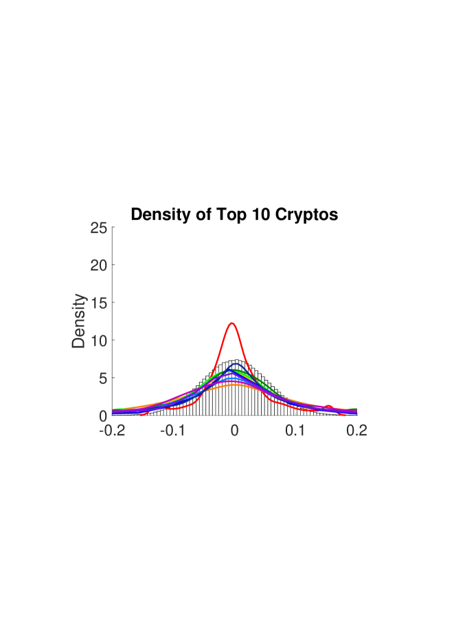
Figure 7: Density of daily log returns of the top 10 CCs (DOGE, ZET, XMG, SYS, POT, DGC, DMD, RBY, START, EMC2) against a normal distribution with same mean and variance. The time span is from 2016-01-01 to 2019-12-31.

A strong limitation of Markowitz-based portfolio strategies lies in the assumption of Gaussian distributions of assets’ log-returns. Absent those, for investors whose preferences are not fully described by a quadratic utility funcion, variance or volatility is an insufficient risk measure, leading the MV strategy to give a non-optimal portfolio composition. Importantly, returns of CCs have even heavier tails as compared to those of equities, as detailed in chuen2017cryptocurrency (30) and elendner_cross-section_2017 (39). The descriptive statistics of our investment universe in Figure 7 and Table 9 in Appendix 9.2 again provide strong evidence of this heavy-tailed distributions for CCs. Therefore, we include a strategy that accounts for higher moments via Conditional Value at Risk (CVaR): we include a Mean-CVaR-optimized portfolio as in rockafellar2000optimization (92, 67).

For a given $\alpha<0.05$ risk level, the CVaR-optimized portfolio weights $w$ are derived as:

$$\underset{w\in\mathbb{R}^{N}}{\text{min}}\text{CVaR}_{\alpha}(w),\hskip 5.69054pt\text{s.t. }\mu_{P}(w)=r_{T},w^{\top}1_{p}=1,w_{i}\geq 0,$$ (2)

$$\text{CVaR}_{\alpha}(w)=-\frac{1}{1-\alpha}\int\displaylimits_{w^{\top}X\leq-\text{VaR}_{\alpha}(w)}w^{\top}Xf(w^{\top}X|w)dw^{\top}X,$$ (3)

with $\frac{\partial}{\partial w^{\top}X}F(w^{\top}X|w)=f(w^{\top}X|w)$ the probability density function of the portfolio returns with weights $w$. $\text{VaR}_{\alpha}(w)$ is the corresponding $\alpha$-quantile of the cumulative distribution function, defining the loss to be expected in $(\alpha\cdot 100)\%$ of the times.

As for the MV portfolio, we construct the efficient frontier, from which to derive the portfolios to add to our analyses. As a risk-oriented strategy, we add the MinCVaR strategy, minimizing the risk in terms of CVaR. As far as a return-oriented strategy is concerned, given our methodology, the maximal expected return arises in the same way as in the maximum-return portfolio (“RR-MaxRet” in Table 1), by investing in the riskiest asset only. Thus, we report this portfolio only as RR-MaxRet.

3.1.4 Risk-parity portfolio (with equal risk contribution, ERC)

One traditional risk-based portfolio strategy is based on the concept of risk parity. The underlying idea is to set weights such that each asset has the same contribution to portfolio risk, see qian2005financial (90). maillard2010properties (73) derive properties of such portfolios and rename them “equal-risk-contribution” (ERC) instruments. The Euler decomposition of the portfolio volatility $\sigma_{P}(w)=\sqrt{w^{\top}\Sigma w}$ (hardle_applications_2015, 50) allows to present it in the following form:

$$\sigma_{P}(w)\stackrel{{\scriptstyle\operatorname{def}}}{{=}}\sum_{i=1}^{N}\sigma_{i}(w)=\sum_{i=1}^{N}w_{i}\frac{\partial\sigma_{P}(w)}{\partial w_{i}},$$ (4)

where $\frac{\partial\sigma_{P}(w)}{\partial w_{i}}$ is the marginal risk contribution and $\sigma_{i}(w)=w_{i}\frac{\partial\sigma_{P}(w)}{\partial w_{i}}$ is the risk contribution of the $i$-th asset. So, to construct the ERC portfolio, we calibrate:

$$\sigma_{i}(w)=\frac{1}{N}\quad\forall i$$ (5)

The ERC portfolio can be compared to the EW portfolio: instead of allocating capital equally across all assets, the ERC portfolio allocates the total risk equally across all assets. Consequently, if variances of log-returns were all equal, the ERC portfolio would become identical to EW portfolio. The ERC portfolio is also comparable to the MinVar portfolio, which focuses on parity of marginal contributions of all assets.

3.1.5 Maximum-diversification portfolio (based on the Portfolio Diversification Index, PDI)

Originally, the Maximum Diversification portfolio (MD) uses an objective function introduced in choueifaty2008toward (25) that maximizes the ratio of weighted average asset volatilities to portfolio volatility or diversification ratio as in Equation (22). In our study, instead of the diversification ratio we maximize the Portfolio Diversification Index (PDI) proposed by rudin2006portfolio (95). It consists in assessing a Principal Component Analysis (PCA) on the weighted asset returns’ covariance matrix, i.e., identifying orthogonal sources of variation. In its original form, PDI does not account for the actual portfolio weights, here we incorporate weighted returns. We optimize:

$$\underset{w\in\mathbb{R}^{N}}{\text{max}}\text{ PDI}_{P}(w),\quad\text{s.t. }w^{\top}1_{p}=1,\quad w_{i}\geq 0$$ (6)

$$PDI_{P}(w){=}2\sum_{i=1}^{N}iW_{i}-1,$$ (7)

where $W_{i}=\frac{\lambda_{i}}{\sum_{i=1}^{N}\lambda_{i}}$ are the normalised covariance eigenvalues $\lambda_{i}$ in decreasing order, i.e., the relative strengths. Thus, an “ideally diversified” portfolio, i.e., when all assets are perfectly uncorrelated and $W_{i}=1/N$ for all $i$, then $PDI={N}$. On the contrary a $PDI\approx 1$ indicates diversification is effectively impossible. Thus, in case of perfectly uncorrelated assets the MD portfolio will be exactly the EW portfolio. The PDI summarises the diversification of a large number of assets with a single statistic, and can compare the diversification across different portfolios or time periods.

3.2 Averaging of portfolio models

Additional to individual allocation models, we also consider combinations of models. After all, every individual model is subject to estimation risk; the idea of combining (or averaging) models in order to reduce such risk received attention in various areas, and particularly in forecasting (avramov2002stock, 7). Traditional model-averaging methods use information criteria—like AIC or BIC—to identify relative shares of models. Across portfolio-allocation models the likelihood is unknown, however, therefore we calculate model shares with the loss function $l$, defined as

$$l(w)=w^{\top}\hat{\mu}-\frac{\gamma}{2}w^{\top}\hat{\Sigma}w.$$ (8)

The parameter $\gamma$ reflects the investor’s risk aversion, with $\gamma$ being large (small) for a risk-averse (risk-seeking) investor. We use two approaches to construct combined strategies: Naïve averaging of the portfolio weights, as well as the combination method based on a bootstrap procedure described in schanbacher2014combining (97). However, in order to account for possible time series dependencies at a daily frequency, we apply the stationary bootstrap algorithm of politis1994stationary (88) with automatic block-length selection proposed by politis2004automatic (89).

Consider a set of $m$ asset allocation models. The corresponding portfolio weights per model are given by $W=(w^{1},\dots,w^{m})$. Relative shares of (or beliefs in) individual models are $\pi=(\pi^{1},\dots,\pi^{m})$, such that $\pi^{\top}1_{m}=1$. Then the asset weights for the combined portfolio are given by:

$$w^{comb}=\sum_{i=1}^{m}\pi^{i}w^{i}$$ (9)

The Naïve combination over all asset allocation models just assigns equal shares, i.e., $\pi^{i}_{t}=\frac{1}{m}$ for all $i=1,\dots,m$.

The alternative, more sophisticated approach is to set the share $\pi^{i}_{t}$ equal to the probability that model $i$ outperforms all other models. We apply a bootstrap method to estimate these probabilities. For every period $t$ we generate a random sample (with replacement) of $k$ returns using returns $X_{k(t-1)+1}\dots X_{k(t-1)+1+K}$, i.e., $K$-long returns vectors of the $t-1$ rolling window. We apply all $m$ asset allocation models to these bootstrapped returns. The procedure is repeated $B$ times. Let $s_{i,b}=1$ if model $i$ outperforms in terms of the loss function other models in the $b$-th bootstrapped sample, otherwise $s_{i,b}=0$. The probability of model $i$ being best is then estimated as

$$\hat{\pi}^{i}_{t}=\frac{1}{B}\sum_{b=1}^{B}s_{i,b}$$ (10)

where $B=100$ is our number of independent bootstrap samples, and $s_{i,b}=1$ if model $i$ is the best model in the $b$-th sample.

Model	Reference	Abbreviation
Model-free strategies
Equally weighted	demiguel2009optimal (34)	EW
Risk-oriented strategies
Mean-Variance – min Var	merton1980estimating (77)	MinVar
Mean-CVaR – min risk	rockafellar2000optimization (92)	MinCVaR
Equal Risk Contribution	maillard2010properties (73)	ERC
(Risk-parity)
Maximum Diversification	rudin2006portfolio (95)	MD
Return-oriented strategies
Risk-Return – max return	markowitz_portfolio_1952 (74)	RR-MaxRet
Risk-Return-oriented strategies
Mean-Variance – max Sharpe	jagannathan_risk_2003 (57)	MV-S
Combination models
Naïve Combination	schanbacher2015averaging (98)	CombNaïve
Weight Combination	schanbacher2014combining (97)	Comb

Table 1: List and categorization of all asset allocation models we implement, including their abbreviations and references.

4 Liquidity constraints with the LIBRO framework

In this section, we review the LIBRO framework for portfolio formation, which prevents too high portfolio weights for low-liquidity assets, by introducing weight constraints in the portfolio optimization which depend on liquidity.

Liquidity, however, does not have a unique definition; different concepts and measures abound. wyss_measuring_2004 (114, 111) survey the extensive literature on liquidity measures in equity markets; the literature on CC liquidity is still scarce, with notable exceptions of Brauneis_et_al_2020 (17, 99). Due to the highly fragmented market structure of CC exchanges (no dominant or central exchange is trading all assets), we employ Trading Volume (TV) as our proxy for liquidity. TV is also the basis for the widely used illiquidity measure, and proved suitable for the LIBRO methodology. In principle, alternative measures like the bid-ask spread would also be applicable, as many exchanges report bid and ask prices; however, reliable order-book data aggregated across exchanges and for all CCs is lacking. TV, in contrast, is available for practically all CC markets, and aggregated without problems. For these reasons, we follow trimborn_investing_2017 (109) and employ TV as our liquidity measure. TV is defined as

$$TV_{ij}=p_{ij}\cdot q_{ij},$$ (11)

where $p_{ij}$ is the closing price of asset $i$ at date $j$, and $q_{ij}$ is the volume traded at date $j$ of asset $i$. The liquidity of asset $i$ in period $t$ can then be measured with the sample median of trading volume,

$$TV_{i}=\frac{1}{2}(TV_{i,up}+TV_{i,lo}),$$ (12)

where $TV_{i,up}=TV_{i,\lceil\frac{l+1}{2}\rceil}$ and $TV_{i,lo}=TV_{i,\lfloor\frac{l+1}{2}\rfloor}$.

Define $M$ as the total amount invested in all $N$ assets, so that $Mw_{i}$ denotes the market value held in asset $i$. trimborn_investing_2017 (109) formulate the constraint on the weight of asset $i$ as

$$Mw_{i}\leq TV_{i}\cdot f_{i},$$ (13)

where $f_{i}$ captures the speed with which an investor intends to be able to clear the current position in asset $i$ via multiples of TV. For example, $f_{i}=0.5$ implies the position in asset $i$ must not exceed 50% of median trading volume. It results in a boundary for the weight on asset $i$ as

$$w_{i}\leq\frac{TV_{i}\cdot f_{i}}{M}=\widehat{a}_{i}.$$ (14)

The beauty of this approach lies in its ease to include it into any portfolio optimization.

5 Evaluating the performance of portfolios

While Section 3 presents the set of common asset-allocation models we implement, no unique metric exists to evaluate and compare them. In order to draw conclusions about the effect of adding CCs to broadly diversified portfolios, we pursue three dimensions: First, we calculate a range of widely used performance measures in Section 5.1. Second, in Section 5.2 we run direct tests for differences between strategies on a pair-wise basis. Third and finally, in Section 5.3 we address the diversification effect of CCs directly by calculating three well-known measures of portfolio concentration.

5.1 Performance measures

To assess the performance of the investment strategies we consider as it develops over time, we employ the following five common performance criteria widely used in literature, as well as by practitioners. Performance measures are computed based on the time series of daily out-of-sample returns generated by each strategy.

First, we measure the cumulative wealth (CW) generated by each strategy $i$

$$W_{i,t+1}=W_{i,t}+{\hat{w}_{i,t}^{\top}X_{t+1}},$$ (15)

starting with an initial portfolio wealth of $W_{0}=\$1$. Cumulative wealth, while naturally of high interest as a measure of performance achieved over the period considered, is not sufficient to rank our allocation approaches. Therefore why we also compute two traditional measures of risk-adjusted returns: the Sharpe ratio, and the certainty equivalent. Moreover, we provide the Adjusted Sharpe Ratio (ASR) in order to address the MinCVaR strategy and the non-Gaussian nature of the return distributions.

The Sharpe Ratio (SR) of strategy $i$ is defined as the sample mean of out-of-sample excess returns (over the risk-free rate), scaled by their respective standard deviation. This definition presumes an unambiguous risk-free rate, inexistent in the global context of CCs. Fortunately, our sample period is characterized by most of the global economy at or very close to the zero lower bound on interest rates; so we can sidestep the question by implicitly setting the riskless rate to 0 and defining

$$\widehat{SR_{i}}=\frac{\hat{\mu_{i}}}{\hat{\sigma_{i}}^{2}}.$$ (16)

The Certainty Equivalent (CEQ) captures, for an investor with a given risk aversion $\gamma$, the riskless return that said investor would consider of equal utility as the risky return under evaluation. For the case $\gamma=1$, it is equivalent to the close-form solution of markowitz_portfolio_1952 (74) portfolio optimization problem in Equation (1).

$$\widehat{CEQ_{i,\gamma}}=\hat{\mu_{i}}-\frac{\gamma}{2}\hat{\sigma_{i}}^{2}$$ (17)

While there is debate about the risk-averion coefficient best describing investors going back to Mehra_Prescott_1985 (75), we argue that current CC investors are unlikely to be characterized by extremely high risk aversion, and calculate the CEQ in the empirical part of our paper with a $\gamma$ of $1$. As can be noted, the CEQ corresponds to the loss function $l$ defined in Equation (8).

The CEQ and in particular the SR are more suitable to assess of strategies when assets exhibit normally distributed returns. To address this drawback, pezier2006relative (86) propose the Adjusted Sharpe Ratio (ASR). ASR explicitly incorporates skewness and kurtosis:

$$\widehat{ASR_{i}}=\widehat{SR_{i}}\left[1+\left(\frac{S_{i}}{6}\right)\widehat{SR_{i}}-\left(\frac{K_{i}}{24}\right)\widehat{SR_{i}}^{2}\right]$$ (18)

where $SR_{i}$ denotes the Sharpe Ratio, $S_{i}$ the skewness, and $K_{i}$ the excess kurtosis of asset $i$. Thus, the ASR accounts for the fact that investors generally prefer positive skewness and negative excess kurtosis, as it contains a penalty factor for negative skewness and positive excess kurtosis.

To assess the impact of potential transaction costs associated with asset rebalancing, we also calculate two measures for turnover. Portfolio turnover is computed to capture the amount of trade necessary on rebalancing dates as

$${TO_{i}}=\frac{1}{T-K}{\sum_{t=1}^{T-K}}{\sum_{j=1}^{N}}|\hat{w}_{i,j,t+1}-\hat{w}_{i,j,t+}|$$ (19)

where $w_{i,j,t}$ and $w_{i,j,t+1}$ are the weights assigned to asset $j$ for periods $t$ and $t+1$ and $w_{i,j,t+}$ denotes its weight just before rebalancing at $t+1$. Thus, we account for the price change over the period, as one needs to execute trades in order to rebalance the portfolio towards the $w_{t}$ target. High turnover will imply significant transaction costs; consequently, the lower Turnover of a strategy, the better it performs.

Target turnover, the second turnover-related measure, captures the amount of change in target weights between two consecutive rebalancing dates as

$${TTO_{i}}=\frac{1}{T-K}{\sum_{t=1}^{T-K}}{\sum_{j=1}^{N}}|\hat{w}_{i,j,t+1}-\hat{w}_{i,j,t}|$$ (20)

In contrast to Equation (19), here the difference between weights spans the time interval of one rebalancing period, instead of the (conceptually infinitesimal) duration of rebalancing trades. Therefore, the realized price paths of the assets affect the measure only insofar as they lead to different parameter estimates and thus a revision in target weights. The difference between the two turnover measures is best illustrated by considering the EW strategy: it may require high turnover to return to exactly equal weights per asset every rebalancing date; yet by definition it will never exhibit and target turnover.

5.2 Testing for performance differences between strategies

To test if strategies are significantly different from each other, we provide the $p$-values of pairwise tests. The common approach by jobson1981performance (59) is widely used in the performance evaluation literature (e.g., also in demiguel2009optimal, 34). However, this test is not appropriate when returns have tails heavier than the normal distribution. Therefore, as a testing procedure we rely on the ledoit2008robust (68) test with the use of robust inference methods. We test for difference of both CEQ and SR, and report results for the HAC (heteroskedasticity and autocorrelation) inference version. The procedure is described in Appendix 9.1.

5.3 Measuring diversification effects

To evaluate portfolio concentration and portfolio diversification effects, we calculate three measures: a) the Portfolio Diversification Index (PDI) as in introduced in Equation (7), b) Effective N as introduced by strongin2000beating (107), and c) the Diversification Ratio.

Effective N is defined as

$$N_{\textit{eff}}(w_{t})=\frac{1}{\sum_{j=1}^{N}{w^{2}_{j,t}}}$$ (21)

with $j=1,\dots,N$ indexing assets. Effective N varies from 1 in the case of maximal concentration, i.e., the portfolio entirely invested in a single asset, to $N$—its maximum achieved by an equally-weighted portfolio. The design of Effective N is related to other traditional concentration measures, e.g., the Herfindahl Index, the sum of squared market shares to measure the amount of competition. Effective N can be interpreted as the number of equally-weighted assets that would provide the same diversification benefits as the portfolio under consideration.

The diversification ratio, suggested by choueifaty2011properties (26), measures the proportion of a portfolio’s weighted average volatility to its overall volatility:

$$DR(w_{t})=\frac{w_{t}^{\top}\sigma_{t}}{\sqrt{w_{t}^{\top}\Sigma_{t}w_{t}}}=\frac{w_{t}^{\top}\sigma_{t}}{\sigma_{P,t}(w_{t})}$$ (22)

Thus, the diversification ratio has the form of the Sharpe Ratio in Equation (18), with the sum of weighted asset volatilities replacing the expected excess return. In case of perfectly correlated assets, the DR equals 1; in contrast, in a situation of “ideal diversification,” i.e., perfectly uncorrelated assets, $DR=\sqrt{N}$. Hence, in our empirical study we report the results for $DR^{2}$, for two reasons: First, to make it comparable to the other two used metrics, and second, because choueifaty2008toward (25) demonstrate that for a universe of $N$ independent risk factors, the portfolio that weighted each factor by its inverse volatility would have a $DR^{2}$ equal to $N$. Hence $DR^{2}$ can be viewed as a measure of the effective degrees of freedom within a given investment universe.

6 Data

For the empirical analysis, we collect daily price data on a sample of CCs and traditional financial assets (including alternative investments) over the period 2015-01-01 to 2019-12-31 (1304 daily log-returns). CC prices are provided by CoinGecko, data for traditional assets is acquired from Bloomberg. Many CCs were established only after January 2015, or ceased to trade prior to the period we study. Since investors who apply rules-based optimization techniques usually only consider assets with sufficient price histories, we require CCs to have a continuous return time-series over the period of our study in order to be included. By excluding coins that did not already circulate in January 2015, went extinct before December 2019, or have only patchy price series, we effectively focus on solid CCs, of interest to investors considering positions in this novel asset class. We also sidestep ICOs. Hence, our final data sample for portfolio construction includes 52 CCs next to 16 traditional assets. In order to cover 3 different reallocation frequencies (daily, weekly, monthly), we calculate with daily, weekly and monthly return series for all assets treated equally.

We employ a rolling-window approach for the portfolio construction. The initial portfolio weights are determined from estimations based on the first year (2015), after which we ‘roll’ through the dataset by estimating new portfolio weights at the reallocation frequency. Depending on the employed frequency approach, this adds one day, week, or month of data to the estimation set and leaves out the oldest day, week or month of data, in order to capture potentially time-varying parameters.

To evaluate the performance of each of the strategies we consider, our research question studies the effects of including CCs as an addition to classical, well-diversified portfolios. Therefore, our investment universe always includes 16 traditional assets from 5 asset classes: equity, fixed-income, fiat currencies, commodities, and real estate. Since CCs are global in nature, our traditional assets cover the 5 main economic areas around the globe (Europe, USA, UK, Japan, China). In this way, the asset space is sufficiently broad to allow diversification without CCs, ensuring any relevance of CCs we find is genuine, and at the same time is still narrow enough to allow us to add each CC individually as an asset without leading to high-dimensionality issues in covariance estimation. The full list of traditional constituents of the investment universe is provided in Table 2. Tables 9 and 8 in Appendix 9.2 report summary statistics of all constituents considered in our empirical study.

The main properties of our data correspond to the findings of the prior literature, e.g., chuen2017cryptocurrency (30): CCs outperform traditional asset classes in terms of average daily realised returns, their returns exhibit higher volatility, with means mostly positive while the medians are mostly negative, positive movements occur less frequently than negative ones, but with higher magnitudes (absolute values of minima and lower deciles are less than of maxima and higher deciles for the majority of CCs). Correlation analysis of the top 5 CCs by market capitalization with traditional asset classes shows the potential of CCs to increase diversification: As can be seen from Table 7, correlation coefficients with none of the traditional assets exceed $0.1$.

Name	Asset class
EURO STOXX 50	Equity
S&P100	Equity
NIKKEI225	Equity
FTSE100	Equity
SSE (Shanghai Stock Exchange) index	Equity
MSCI ACWI COMMODITY PRODUCERS	Commodities
GOLD	Commodities
FTSE EPRA/NAREIT DEV REITS	Real Estate
EUR/USD	Fiat currency
GBP/USD	Fiat currency
CNY/USD	Fiat currency
YEN/USD	Fiat currency
Eurozone 10Y Gov Bonds	Fixed income
UK 10Y Gov Bonds	Fixed income
USA 10Y Treasuries	Fixed income
Japan 10Y Gov Bonds	Fixed income

Table 2: List of traditional constituents of the investment universe. Note that we term all these asset classes, including alternative assets, “traditional” in order to contrast them with investments in cryptocurrencies (CCs). We obtain price series for all traditional investments from Bloomberg.

7 Empirical results

In this section we evaluate the out-of-sample performance of the portfolio allocation strategies in order to address Questions 1–6. We analyze two dimensions: First, how does risk-adjusted performance compare across different strategies and performance measures? Second, which diversification benefits are generated by each method?

7.1 Including CCs in portfolios: performance effects

The first step of our performance analysis examines how adding CCs to a portfolio affects efficient frontiers. In principle, the efficient frontier is unique, thus identical for all allocation strategies. However, it depends on the risk measure (variance or CVaR in this paper), as well as on whether liquidity constraints are enforced (via LIBRO in this paper) or not.

Our second step then addresses the performance comparison across portfolio strategies, in terms of cumulative wealth as well as popular risk-adjusted measures.

Figure 1: Efficient frontiers surfaces: the first column displays the frontiers for portfolios with only traditional assets (including alternative investments, but no cryptocurrencies, CCs) as constituents, the second column adds CCs without liquidity constraints, and the third column instead adds only CCs up to a liquidity constraint (via the LIBRO approach with an investment sum of USD 10 mln). The top row depicts frontiers from mean-variance optimization, the lower one from mean-CVaR optimization. All frontiers are built on a daily basis and plotted over the period from 2016-01-01 to 2019-12-31.

CCPEfficient_surface

7.1.1 Efficient frontiers

Figure 1 plots efficient frontiers for three groups of assets: only traditional assets, traditional assets & CCs without liquidity constraints, and traditional assets & liquid CCs, up to the constraint defined via the LIBRO approach with an investment sum of USD 10 mln. The top row depicts frontiers from mean-variance optimization, the lower three panels are based on mean-CVaR-optimal allocations. All panels show frontiers built on a daily basis, evolving over time.

For both optimization rules, including CCs leads to a distinct extension of the frontiers: for low levels of risk, portfolios with CCs give a similar level of return as without them, but much higher expected returns can be sought when CCs are included. The second important observation is that mean-variance frontiers, in most cases, are shorter than mean-CVaR frontiers (the same level of returns has lower variance than CVaR), evidence of risk not being inadequately captured by variance, in line with expectations. The LIBRO approach shortens the frontiers especially in the beginning of the investment period, because it limits the influence of turbulently growing CCs with low trading volumes. At the same time, it is visible that starting roughly in January 2017, the difference between frontiers with (LIBRO) and without constraints all but vanishes—a change driven by the extreme growth of trading volumes together with capitalisation of the entire CC market during that boom period.

The CC market crash in early 2018 is also clearly visible as the frontiers collapse. At the trough, series of strongly negative returns amidst high volatility and evaporating liquidity lead to CCs playing close to no role in optimal portfolios. As the market consolidates, in 2019 CCs again pick up their role in extending the efficient frontier: however, until today the discrepancy between portfolios with and without concern for liquidity considerations remains pronounced. Consequently, the importance of limiting exposure to illiquid CCs remains high. Portfolio optimization without liquidity constraints may promise an attractive performance in theory which it cannot realize in the market.

7.1.2 Comparing strategies via performance metrics

First we examine cumulative wealth, produced by the allocation strategies we study. Figures 2 and 3 display the dynamics of cumulative wealth for eight of the strategies considered, with and without enforcing liquidity constraints, respectively. As benchmarks we also plot S&P100, EW, MV-S and MinVar portfolios built only from traditional investment constituents (Traditional Assets, “TrA”). The EW strategy is displayed separately in Figure 4, and discussed subsequently. Table 3 summarizes all performance indicators.

The following conclusions can be drawn regarding final Cumulative Wealth (CW) over the entire period of our study when ignoring liquidity: despite CCs trading far below their historical peaks at the end of our time span, most portfolios with CCs generally outperform benchmark portfolios with only conventional constituents. However, the discrepancies across strategies are huge, and the worst-performing strategy RR-MaxRet, which invests always in the asset with the highest expected return (and thus most often in a CC), ends up with what can be called a catastrophic result: over the four years of our study, it loses 97% of its initial wealth by the end of 2019. Critically, the strategy did provide stellar results during the boom phase of 2017, exceeding a multiple of 20 times initial wealth at its peak. Yet clearly, historical returns were no long-term predictor of expected returns for the best-performing CCs, and the lack of diversification hurt this strategy badly.

On the other end of the spectrum, the highest result is achieved by MD, with an accumulated final wealth of 275%. This amounts to an annualized rate of return of just below 30% over a 4-year period in which the S&P100 lost 10%. Critically, this result is also achieved by investing in small CCs (and therefore also follows the boom-and-bust cycle to a comparable degree): the difference is driven by the very strong diversification the MD strategy pursues by design. It is therefore not surprising that ERC turns out the second-best strategy, with a +22% return over the period. Its construction successfully limits its exposure to the extremes during 2017/18 to about an order of magnitude lower than MD.

Regarding the combined strategies, the naïve version is strongly susceptible to RR-MaxRet, while the bootstrapped version performs quite well.

Finally, the model-free EW strategy with CCs underperforms with a final loss of 13%, while equal weighting across only traditional assets achieves the best performance among the benchmark strategies. However, Figure 4 shows how EW performance exhibits high variation over the time span, similar in nature to MaxRet and MD. The figure displays MD and EW separately, to elucidate two important points: first, how disproportionately the performance of small coins exceeded the gains of established CCs in the 2017 price explosion; second, how seriously calculated results of portfolio allocation rules can diverge from returns achievable by investors if lack of liquidity is not taken into account.

Generally, LIBRO portfolios have mixed results in terms of cumulative wealth. Most importantly, MD underperforms when enforcing LIBRO constraints. Of course, this implies that the high performance of unconstrained optimization can only be reached for very small investment sums. For larger portfolios, when the liquidity constraints turn binding, performance need not necessarily suffer. By limiting the exposure to individual (and thus also small) coins, some strategies, including RR-MaxRet, are positively affected by LIBRO. When ignoring the liquidity risk, this strategy retained 3% of its initial value; with LIBRO it retains 59.1%. Also the combined strategy COMB, which provides a positive performance without LIBRO, further improves by 8.6% when protecting the portfolio from liquidity risk.

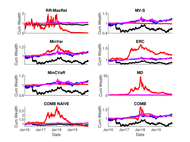
Figure 2: Performance in terms of cumulative wealth of portfolio strategies without liquidity constraints with monthly rebalancing ($l=21$) over the period from 2016-01-01 to 2019-12-31 with the following colour code: S&P100, EW–TrA, RR-MaxRet–TrA and the corresponding allocation strategy from Table 1. “TrA” denotes only traditional, i.e., non-CC assets are included. Note that the date axes are aligned, but the wealth axes are not, due to large disperion in scales.

CCPPerformance

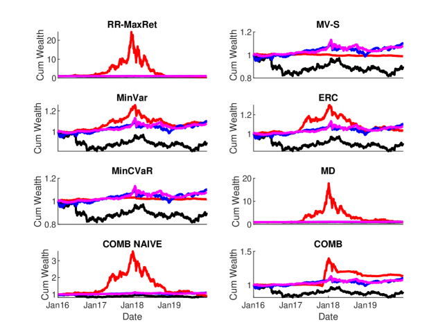
Figure 3: Performance in terms of cumulative wealth of portfolio strategies with liquidity constraints (based on LIBRO at the level of USD 10 mln) and monthly rebalancing ($l=21$) over the period from 2016-01-01 to 2019-12-31 with the following colour code: S&P100, EW–TrA, RR-MaxRet–TrA and the corresponding allocation strategy from Table 1. “TrA” denotes only traditional, i.e., non-CC assets are included. Note that the date axes are aligned, but the wealth axes are not, due to large disperion in scales.

CCPPerformance

Allocation	Portfolio performance measures: monthly rebalancing
Strategy	CW		SR		ASR		CEQ		TO		TTO
	No const	10 mln	No const	10 mln	No const	10 mln	No const	10 mln	No const	10 mln	No const	10 mln
Benchmark strategies
S&P100	$0.900$	$0.900$	$-0.016$	$-0.016$	$-0.016$	$-0.016$	$0.000$	$0.000$	$0.000$	$0.000$	$0.000$	$0.000$
EW TrA	$1.102$	$1.102$	0.033	0.033	0.033	0.033	$-0.001$	$-0.001$	$3.615$	$3.615$	$0.000$	$0.000$
MV-S TrA	$1.076$	$1.076$	$0.028$	$0.028$	$0.028$	$0.028$	$0.000$	$0.000$	$2.199$	$2.199$	$0.274$	$0.274$
EW	$0.877$	$0.877$	$-0.003$	$-0.003$	$-0.003$	$-0.003$	$-0.001$	$-0.001$	$4.345$	$4.345$	$0.000$	$0.000$
Risk-oriented strategies
MinVaR	$0.990$	$0.990$	$-0.041$	$-0.011$	$-0.041$	$-0.011$	$-0.007$	$-0.002$	$8.541$	$7.672$	$0.056$	$0.056$
MinCVaR	$1.021$	$1.018$	$0.026$	$0.023$	$0.026$	$0.023$	$0.000$	$0.000$	$14.884$	$8.093$	0.112	0.114
ERC	$1.224$	$1.035$	0.033	$0.009$	0.033	$0.009$	$0.000$	$0.000$	$4.193$	$9.840$	$0.058$	$0.064$
MD	2.751	$0.858$	$0.020$	$-0.003$	$0.020$	$-0.003$	$0.000$	$-0.001$	$20.315$	$48.707$	$0.391$	$0.209$
Return-oriented strategies
RR-MaxRet	$0.030$	$0.591$	$-0.015$	$-0.016$	$-0.015$	$-0.016$	$0.000$	$0.000$	0.687	0.731	$0.687$	$0.479$
Risk-Return-oriented strategies
MV-S	$1.090$	$1.096$	$0.024$	$0.028$	$0.024$	$0.027$	$0.000$	$0.000$	$4.021$	$8.591$	$0.291$	$0.290$
Combination of models
COMB NAÏVE	$0.716$	$0.908$	$-0.015$	$-0.005$	$-0.015$	$-0.005$	$-0.001$	$0.000$	$3.553$	$36.731$	$0.211$	$0.156$
COMB	$1.048$	1.134	$0.010$	$0.029$	$0.010$	$0.029$	$0.000$	$0.000$	$6.758$	$5.759$	$0.148$	$0.145$

Table 3: Performance measures for all investment strategies as well as benchmarks over the entire time period from 2016-01-01 to 2019-12-31, with monthly rebalancing ($l=21$). The performance measures are final cumulative wealth (CW), the Sharpe ratio (SR), the adjusted Sharpe ratio (ASR), the certainty equivalent (CEQ), and turnover. “TrA” denotes only traditional, i.e., non-CC assets are included. Strategies are detailed in Table 1. Highest results are highlighted in red. 

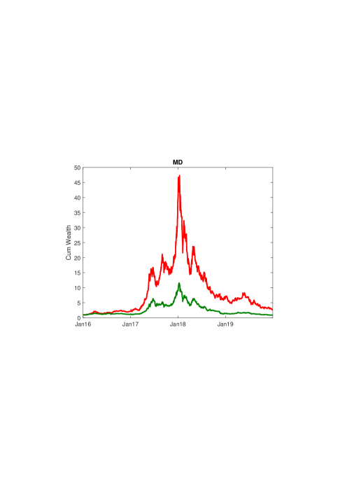
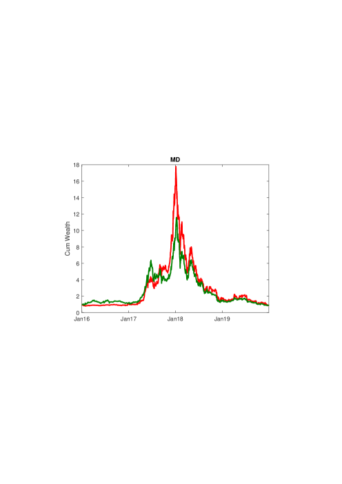
Figure 4: Performance in terms of cumulative wealth of portfolio strategies of the maximum-diversification strategy (MD) without (left panel) and with (right panel) liquidity constraints (based on LIBRO at the level of USD 10 mln), with monthly rebalancing ($l=21$) over the period from 2016-01-01 to 2019-12-31. For reference, the equally-weighted EW strategy is displayed. Note that the date axes are aligned, but the wealth axes are not, due to large disperion in scales.

Allocation strategy		1	2	3	4	5	6	7	8	9	10	11
1	S&P100
2	EW-TrA
3	EW
4	RR Max Ret
5	MV-S
6	MinVar
7	ERC
8	MinCVaR
9	MD
10	COMB NAÏVE
11	COMB

Table 4: Tests for difference between the Sharpe ratio SR (lower triangle) and the certainty equivalent (CEQ, upper triangle) of all strategies with respect to each other: color-coded $p$-values with significance at the 0.01, 0.05 and 0.1 level (without liquidity constraints).

CCPTests

Figure 5: Evolution of the portfolio composition (i.e., relative weights) of all allocation strategies (without liquidity constraints) with monthly rebalancing over the period from 2016-01-01 to 2019-12-31: the black line separates conventional assets (“TrA,” upper yellow part of the spectrum) from cryptocurrencies (CCs, lower green-blue part of the spectrum).

CCPWeights

Figure 6: Evolution of the portfolio composition (i.e., relative weights) of all allocation strategies with a position limit of USD 10 mln (via the LIBRO approach) with monthly rebalancing over the period from 2016-01-01 to 2019-12-31: the black line separates conventional assets (“TrA,” upper yellow part of the spectrum) from cryptocurrencies (CCs, lower green-blue part of the spectrum).

CCPWeights

Next, we analyse risk-adjusted performance for all portfolios. While MD demonstrates superior absolute performance, ERC dominates in terms of risk-adjusted performance, in particular in terms of its (adjusted) Sharpe Ratio of $0.033$. Importantly, turnover is much lower at $4.2$ (unconstrained, constrained: $9.8$), slightly below that of EW and above MV-S. Turnover and target turnover per strategy are reported in the last four columns in Table 3, which show that the only strategy with appreciably lower trading is RR-MaxRet at $0.69$ (constrained: $0.73$), with the above-mentioned harsh result. This is expected, given that the strategy is by construction the most concentrated one, consisting of the one asset with the highest return (see also Figures 5 and 6).

It is interesting to note that for the strategies with strong diversification, in particular MD and ERC, but also MV-S, enforcing the LIBRO constraints leads to higher turnover. This is of concern to investors, as it prompts higher transaction costs. At first sight this observation appears counterintuitive, as restricted weights could be expected to reduce trading needs (due to positions partially remaining at their binding limits). The puzzle is explained by the last two columns, reporting target turnover: clearly, changes in target weights are mitigated via the liquidity constraints, corresponding to intuition. At the same time, it is exactly small and illiquid CCs which exhibit the largest volatility, and thus prompt larger trades when at the next rebalancing date positions are brought back to target weights. Enforcing LIBRO constraints leads to positions in more (and prone to be smaller) CCs, triggering larger rebalancing needs in terms of portfolio turnover.

Finally, Table 4 reports when the differences between strategies in terms of CEQ or SR are significant, based on tests described in Appendix 9.1. Although MD, COMB, and in particular MV-S have SR and CEQ higher than the EW strategy, tests do not support significance of this difference. In constrast, the ERC portfolio exhibits a higher SR and this difference is significant. The comparison of risk-adjusted metrics for MinVar and MinCVaR reveals that they differ significantly from each other—testament to the strong deviation of CC returns from the normal distribution. MinCVaR also differs significantly from the diversifying strategies MD and ERC.

As a robustness check, we also conduct all analyses for weekly and daily rebalancing of portfolios. Results are provided in Appendix 9.4, generally confirming the conclusions so far, and show that the qualitative results are robust with regard to the rebalancing frequency.

7.2 Including CCs in portfolios: diversification effects

We separately analyse diversification characteristics of the allocation rules for two reasons: On the one hand, CCs are known from the literature for their diversifying properties; on the other hand, the most diversifying strategies MD and ERC performed best. First, we examine the composition of the optimal portfolios over time. Second, we run mean-variance spanning tests in order to establish if CCs are a valuable addition to broadly diversified portfolios of traditional assets. Third, we analyse diversification across the portfolio strategies by means of dedicated diversification measures.

7.2.1 Portfolio composition

Figures 5 and 6 plot the evolution of portfolio constituents across time, without and with liquidity constraints, respectively. At each date on the abscissa, the simplex of weights is color-coded vertically, with traditional assets on the light end of the spectrum and CCs towards the dark end; a black lines indicates the boundary between the two groups. We can see wide variation in the extent to which the strategies rely on CCs: MaxRet and MD are prone to invest heavily in CCs, while risk-oriented strategies like MinVar and MinCVaR hardly include any. The risk-return-oriented strategy MV-S employs CCs conservatively, yet it does reach at times noteworthy allocations even against the background of such a well-diversified portfolio of traditional assets. The share of CCs is lower in the last 2 years of the time period, but does not drop to zero.

Most importantly, the figures point out how the LIBRO approach, as expected, significantly affects portfolio weights; the most visible difference arises for models with a high share of CCs, namely MD and RR-MaxRet, but also ERC, where it mitigates the exposure particularly in the first half of the investment period.

The weights distribution of the COMB portfolio undergoes quite pronounced changes over the investment period: from high concentration of traditional assets to high concentration of CCs, and back—confirming that no individual model outperforms its competitors permanently.

To shed more light on how these weights affect the performance of each strategy’s portfolio, we also compare the risk structures for all strategies in Figures 8 and 9. After all, the volatility structure of CCs leads to disproportionate risk contributions relative to their capital weights: traditional assets affect changes in portfolio values to a visibly lower degree.

7.2.2 Mean-variance spanning

In order to investigate the impressions from the efficient-frontier plots in Section 7.1.1, we conduct two mean-variance spanning tests on each of the 52 CCs: first, the corrected test of (HK, huberman1987mean, 55), second the step-down test by kan2012tests (61).

Cryptocurrency	F-Test	F-Test1	F-Test2
BCN	3.28	1.23	5.32
	(0.04)	(0.27)	(0.02)
DOGE	1.73	0.01	3.46
	(0.18)	(0.92)	(0.06)
EAC	1.70	0.09	3.32
	(0.18)	(0.76)	(0.07)
NLG	2.79	4.31	1.26
	(0.06)	(0.04)	(0.26)
PPC	3.19	0.61	5.78
	(0.04)	(0.44)	(0.02)
XMG	1.86	3.44	0.28
	(0.16)	(0.06)	(0.60)
XRP	1.88	0.83	2.93
	(0.16)	(0.36)	(0.09)

Table 5: Spanning Tests for individual cryptocurrencies with respect to the efficient frontier constructed from all traditional investment assets, including alternative assets (see Table 2 for a complete list; $p$-value in parentheses). F-Test refers to the corrected test of huberman1987mean (55), $F_{1}$ and $F_{2}$ to step-down tests by kan2012tests (61), testing for spanning of tangency portfolios and for global minimum portfolios, respectively. Only CCs for which at least one test rejects spanning at the 10% level are reported.

Table 5 lists only CCs with at least one test rejecting the hypothesis that traditional assets span the frontier at the 10% level. Recall that our definition of traditional assets includes a broad set of alternative investments, all but CCs. The corrected HK test rejects spanning for 3 CCs. In contrast, the step-down test provides information on the source for spanning rejection: $F_{1}$ tests for spanning of tangency portfolios, whereas $F_{2}$ tests spanning for global minimum portfolios. From Table 5, we see that the $F_{1}$ test rejects spanning for only 2 CCs, pointing out that tangency portfolios which include CCs are significantly different from the benchmark tangency portfolio, but also that the inclusion of the two years 2018–19 has dramatically reduced that number from previously 27 CCs, which included Bitcoin (BTC), Ripple (XRP), Dash (DASH) and Litecoin (LTC). $F_{2}$ rejects spanning for 5 CCs for the entire time period, still including one of the coins with the highest market capitalisation, XRP. Thus, we conclude there still exists evidence that a MV-S portfolio can be improved by 7 out of 52 CCs, but that the integration of CC with financial markets has progressed markedly. Anecdotal evidence in line with this finding comes from the recent outbreak of the corona-virus pandemic, when initially CC markets moved for the first time with strong positive correlation together with financial markets, driven by institutional investors rebalancing in favor of cash holdings, before CCs resumed their diversifying role in subsequent weeks.

Also, but there is little evidence that a MinVar portfolio can be improved. This result is supported by the dynamics of the portfolios’ composition presented in Figures 5 and 6 for unconstrained and LIBRO portfolios, respectively: MinVar portfolios in both cases are constructed entirely from traditional assets, whereas MV-S portfolios have a (varying) CC component throughout the whole investment period.

In sum, the results imply that investors should consider a broader selection of CCs (see Question 3), not only BTC. However, only a small fraction of CCs continue to improve the efficient frontier.

7.2.3 Diversification metrics across portfolio strategies

Table 6 reports results on our three chosen diversification metrics (detailed in Section 5.3). As expected, for the RR-MaxRet strategy there are no diversification benefits—by definition it consists of only one asset at a time (unless LIBRO forces it into more than one asset). The range of values across diversification metrics emphasizes that diversification has different aspects and its quantification depends on the definition used. Consequently, different measures do not always provide identical conclusions about the diversification effects of CCs in portfolios. For instance, in terms of a $DR^{2}$ of $13.73$ ($13.44$), MinCVaR is characterized as most diversified strategy. Slightly lower measures pertain for MinVar and ERC portfolios with $12.02$ ($11.72$) and $8.71$ ($9.41$), respectively. The MD portfolio is a special case regarding this type of diversification, with $DR^{2}$ of $2.64$ ($2.07$) and at the same time a PDI of $21.06$ ($21.01$). Clearly PDI highest for the MD portfolio because of its objective function, maximizing diversification via the number of independent sources of variation in the portfolio.

Allocation	Portfolio diversification effects: monthly rebalancing
Strategy	$DR^{2}$		Effective $N$		PDI
	No const	10 mln	No const	10 mln	No const	10 mln
Benchmark strategies
MV-S TrA	$5.39$	$5.39$	$3.11$	$3.11$	$4.92$	$4.92$
Return oriented strategies
RR-MaxRet	$1.00$	$1.00$	$1.00$	$1.48$	$1.00$	$1.00$
Risk-oriented strategies
MinVar	$12.02$	$11.72$	$2.68$	$2.69$	$20.60$	$20.60$
ERC	$8.71$	$9.41$	17.16	13.61	$20.62$	$20.62$
MinCVaR	13.73	13.44	$3.15$	$3.15$	$20.60$	$20.61$
MD	$2.64$	$2.07$	$3.99$	$3.17$	21.06	21.01
Risk-Return-oriented strategies
MV-S	$8.03$	$7.48$	$3.26$	$3.35$	$20.62$	$20.62$
Combination of models
COMB NAÏVE	$3.43$	$3.62$	$11.60$	$10.92$	$20.65$	$20.67$
COMB	$10.00$	$9.44$	$3.39$	$3.40$	$20.61$	$20.61$

Table 6: Measures of diversification for all investment strategies and a benchmark, over the entire time period from 2016-01-01 to 2019-12-31, with monthly rebalancing ($l=21$). $DR^{2}$ denotes the squared diversification ratio, PDI the portfolio diversification index; all three measures are detailed in Section 5.3. “TrA” denotes only traditional, i.e., non-CC assets are included. Strategies are detailed in Table 1. Results without liqudity constraints (columns “No const”) are contrasted with those when applying LIBRO with a threshold of USD 10 mln (column “10 mln”). Highest results are highlighted in red.

The ERC portfolio is characterized by the highest Effective $N$ of $17.16$ ($13.61$) by a large margin, also a typical result (see, e.g., clarke2013risk, 31) due to its nature: it includes all assets by definition. Apart from MaxRet, the lowest Effective $N$ of $2.68$ ($2.69$) arises for the MinVar portfolio, containing only traditional assets, showing that fewer than $3$ equally-weighted stocks would provide the same diversification by this measure. All other individual strategies also exhibit Effective $N$ ranging between 3 and 4. One more remarkable result concerns the combined portfolios’ concentration: While COMB’s Effective $N$ lies in the range of individual strategies, COMB Naïve exceeds $10$ both in constrained and unconstrained portfolios. In terms of $DR^{2}$, the combined strategies rank inversely, reaching $3.43$ ($3.62$) for COMB Naïve and $10.0$ ($9.44$) for COMB; their PDIs are similar to those of the other risk-oriented portfolios MinVar, MinCVaR and ERC.

Note that with the exception of ERC liquidity constraints do not strongly affect the diversification features of portfolios: all metrics display only minor changes. This result is due to the fact that LIBRO generally lowers the weight of constituents, but does not completely exclude them.

We particularly highlight the difference of diversification of the MV-S portfolios with and without CCs: diversification measured by $DR^{2}$ increases through the inclusion of CCs from $5.39$ ($5.39$) to $8.03$ ($7.48$), and PDI scales up even more strongly, from $4.92$ ($4.92$) to $20.62$ ($20.62$). Thus, the inclusion of CCs remarkably improves portfolio diversification, especially in terms of the distribution of principal portfolio variances.

7.3 Interpretation of the results

In this section we relate our empirical results to the Questions 1–6, along which the contribution of this paper is structured.

Question 1: For whom is investing in the CC market valuable? Is the benefit derived from adding CCs to a portfolio dependent on the investor’s objectives (e.g., return-oriented or diversification seeking)?

As the efficient frontiers in Figure 1 clearly show, the main benefit of CCs accrue to investors who make use of the high-risk/high-return character of their returns; investors with low risk tolerance benefit least. While it is not surprising that CCs constitute risky investments, Figure 5 shows how the risk-oriented strategies (minimizing variance or CVaR) consist almost entirely of traditional assets, so CCs have no influence on them; at least a risk-return orientation is necessary for CCs to play a noteworthy and permanent role in portfolios. At the other end of the specturm, the extremely CC-affine MaxRet strategy, despite stellar performance during the boom phase of 2017, was all but wiped out by the end of our period (ultimately retaining only 3% of its initial value).

The model-free EW strategy is a special case: its performance in the middle of our time period was extraordinary, and so was its collapse when the 2017 price rally in CCs disintegrated. As with MaxRet, both parts are driven by the high weight of small CCs—these were precisely the ones that gained disproportionately in value during the price rally, and subsequently suffered the severest. Therefore, over our complete time span the EW portfolio in fact lost $12.3\%$ in value, whereas other types of investors ended up with gains.

By far the best performance was achieved by investors who target strong (or even maximal) diversification. These strategies, ERC and MD, lead to sizeable exposures to a broader cross-section of CCs, while they limit the risks the EW strategy incurs.

The general conclusion is that the utility from adding CCs to a portfolio strongly depends on the investor’s objective. In particular investors targeting a well-diversified portfolio while willing to bear some risk are advised to consider CCs for their investments.

Question 2: To which type of investor are CC investments most useful? Only professional traders who rebalance their portfolio frequently, or also less actively trading retail investors?

The rebalancing frequency (whether portfolio positions are traded daily, weekly, or monthly to react to market developments by updating estimates and to revert positions to target weights) does influence the performance of investors’ portfolios. For instance, over our study period cumulative wealth for the MV-S strategy grows by 5% when readjusting the portfolio on a daily basis, by 12% with weekly, and 9% with monthly position changes. These difference become more pronounced when transaction costs are deducted, as turnover is naturally higher at a higher rebalancing frequencies. For the RR-MaxRet strategey, the loss attenuates with weekly and exacerbates with daily reallocations.

However, the overall picture does not change across rebalancing frequencies: Even with a more frequent reallocations, still diversification-seeking investors (ERC and MD) significantly outperform the other investment strategies. Therefore, our general conclusions about the effect of adding CCs into investment portfolios do not change qualitatively between daily traders, weekly rebalancing and monthly reallocation (retail investors).

Question 3: Should investors focus on one particular coin (e.g., Bitcoin), a selected few, or rather build a portfolio of a broad selection of CCs?

Most importantly, our findings clearly indicate that diversification also across CCs is beneficial. At the same time, investors could diversify too much. As Table 6 shows, the MD strategy, which had the highest return, showcases an Effective $N$ of only $3.26$. ERC has much higher Effective $N$ of $17.16$, still it features considerably lower final cumulative wealth, at least in unconstrained optimization. Judged by PDI, MD is the most successful strategy, which of course is driven by the fact that the target-weight allocation of MD is derived precisely by maximizing PDI. However, this also indicates that including as many assets in the portfolio as possible is not necessary to adequately represent the covariance matrix, and not beneficial in terms of cumulative wealth.

Figures 5 and 6 caution the interpretation of MD dominating in terms of accumulated returns. Both Figures show that MD includes a broad range of CCs, whereas MinVar and MinCVaR—both with comparable Effective N and PDI—almost entirely exclude them, giving weight only to traditional assets. In this sense we do find evidence that CCs can substitute for traditional assets in portfolio optimization.

Regarding the ERC strategy, while it reaches optimal diversification for the alternative metric of Effective $N$, it provides sizable gains in cumulative wealth and at the same adequately diversifies the portfolio. Figures 5 and 6 indicate that CCs and traditional assets are mixed in the portfolio, while the PDI is close to the one of MD and $DR^{2}$ only second to the pure risk-oriented strategies MinVar and MinCVaR.

Therefore, including CCs to diversify the portfolio is beneficial to achieve high target returns, and balancing traditional assets and CCs is advisable.

Question 4: What exposure to each CC should be held in the portfolio? How informative are past prices, how stable are positions when re-balancing the portfolio? Do model-free strategies like equal-weighting provide reasonable results?

Even though CCs are highly volatile, the past pricing series are informative for portfolio allocation. As such, quantitative methodologies for portfolio allocation are applicable and one is not restricted to non-quantitative or model-free investment schemes. The EW strategy, which we discussed in the answer to Question 1, can exhibit phases of extraordinary returns, but does not manage risk well. At the other end of the spectrum, however, strategies exclusively targeted at lowering risk at all cost do not benefit from CCs. This is of course unsurprising, since lower risk must go at the expense of lesser expected return, most clearly visible already in the efficient frontiers in Figure 1.

Question 5: Can these strategies be implemented in practice? In particular, are all CCs liquid enough for inclusion in an investment portfolio? If not, how can investors still profit from promising CCs with little trading volume without exposing their portfolio too much to illiquidity? Moreover, how is performance affected by honoring such portfolio restrictions?

This question is addressed by LIBRO: The fact that the bounds on CC weights by LIBRO (trimborn_investing_2017, 109) turn out to bind indicates that several CCs are not sufficiently liquid for investors with deeper pockets. Still, the approach allows the inclusion of illiquid CCs up to restricted amounts. This has the positive effect that investors can still perform diversification strategies to quite some degree—strategies that rank among the most profitable. However, the impressive results by strategies with broad CC exposure turn out not to be very scalable. For instance, the MD strategy shows excellent performance without liqudity constraints ($+175\%$), yet the application of LIBRO pushes final CW below initial wealth ($-14\%$).

Clearly, the performance of unconstrained MD profits from unreasonably high weights on small and illiquid CCs. Table 6 illustrates this in terms of Effective $N$ and PDI: MD reaches a very low Effective $N$ of $3.99$, although it includes only CCs, compare the weight composition in Figures 5 and 6. PDI is clearly higher than for other strategies, in line with the objective of MD, and the PDI only shrinks marginally when incorporating LIBRO, whereas Effective $N$ drops by about 1. This implies that the strategy focuses disproportionately on (a) singular CC(s), driving the high returns, which cannot be traded sufficiently for a portfolio of USD 10 mln. At the other end of the spectrum, the mininum-risk strategies focus on traditional assets with high trading volume, therefore they are little affected by LIBRO.

Question 6: Overall, how do the properties of CC returns affect portfolios? Is a certain type of portfolio-allocation method more suitable to manage and simultaneously exploit their properties?

Regarding CC return properties, a lot of prior research exists (see also our literature review in Section 2). We confirm that the patterns of generally high means, high volatilities, excess kurtosis, and low correlations with traditional assets are also present in our sample (see the descriptive statistics in Appendix 9.2). Our contribution addresses the effect of including CCs in already broadly diversified portfolios: Beyond what we have established in the answers to the preceding five questions, our central finding is that the key conclusion of prior studies—that CCs are valuable additions to the investment universe—holds true, but it is critical to mind the limits of quantitative results derived from simplified frameworks. While diversification strategies prove most promising, including only the top CCs foregoes diversification potential. Most importantly, returns of broad CC portfolios that are calculated without accounting for liquidity remain virtual: they cannot be realized by professional investors.

Finally, for certain types of investors, namely those highly risk averse, the benefits can prove too risky to pursue.

8 Conclusion

This study investigates cryptocurrencies as new investment assets available to portfolio management. We investigate the utility gains for different types of investors when they consider cryptocurrencies as an addition to a well diversified portfolio of traditional assets. We consider risk-averse, return-seeking as well as diversification-preferring investors who trade along different allocation frequencies, namely daily, weekly or monthly. To conduct this study, we analyze the performance of commonly used asset-allocation models based on historical prices and trading volumes of 52 cryptocurrencies, combined with 16 traditional assets. The rules-based investment methods cover a broad spectrum of investor objectives, from the classical Markowitz optimization to recent strategies aiming to maximize portfolio diversification. Along with individual portfolio allocation strategies, we also include combined strategies from model averaging. The performance of portfolios is evaluated with a range of different measures, including cumulative wealth, risk-adjusted performance and diversification effects produced by portfolios.

We find that due to the volatility structure of cryptocurrencies, the application of traditional risk-based portfolios strategies, such as equal-risk contribution, minimum-variance and minimum-CVaR, does not boost the performance of investments significantly. In contrast, approaches such as the maximum-return strategy (or strategies with high target returns), and also the maximum-diversification portfolio reach higher expected returns via higher or broader cryptocurrency exposure for investors. As for diversification benefits, we demonstrate an effect beyond well-diversified, global portfolios of conventional assets without CCs. We also document how various rules have different effects on portfolio diversification, depending on the concept of diversification and the chosen measure of its quantification.

Furthermore, following the idea of model averaging and diversification across models, we show that both naive and bootstrap-based combined portfolios exhibit robust high risk-adjusted returns. Portfolios with model-averaged weights achieve significantly higher performance than purely risk-oriented strategies and not significantly lower than the best performing strategies.

We also show how different rebalancing frequencies affect performance, as well as how constraints mitigating liquidity risks of cryptocurrencies (LIBRO) can significantly affect the outcome of strategies that rely on a larger cross-section of CCs. The results remain coherent across all frameworks. Further extensions can be made along three main lines: first, more involved estimators of expected returns and the covariance matrix could be employed; second, more performance measures could be used to evaluate the investment strategies’ results; and third, additional portfolio-allocation strategies could be included in the comparison. In particular, factor-based APT (arbitrage price theory) models would constitute the complementary approach to statistical-optimisation techniques studied in this paper.

9 Appendix

9.1 Test for difference of SR or CEQ between two strategies

We employ the test by ledoit2008robust (68). Let $\nu=(\mu_{i},\mu_{j},\sigma_{i},\sigma_{j})$ denote the vector of the moments of two strategies $i$ and $j$.

Then we can test for a difference of the strategies’ CEQs or SRs via the test statistics defined as the differences of those measures,

$$f_{CEQ}(\nu)=\mu_{i}-\frac{\gamma}{2}\sigma^{2}_{i}-\mu_{j}+\frac{\gamma}{2}\sigma^{2}_{j},$$ (23)

or

$$f_{SR}(\nu)=\frac{\mu_{i}}{\sigma_{i}}-\frac{\mu_{j}}{\sigma_{j}},$$ (24)

respectively.

Applying the delta method yields that if $\sqrt{T-M}(\hat{\nu}-\nu)\xrightarrow{\text{d}}N(0,\Psi)$, then

$$\sqrt{T-M}(\hat{f}-f)\xrightarrow{\text{d}}N(0,\nabla^{\prime}f(\nu)\Psi\nabla f(\nu)),$$ (25)

where $\nabla f$ stands for the derivative of $f$.

The standard error for such a test statistic $\hat{f}$ then amounts to:

$$SE(\hat{f})=\sqrt{\frac{\nabla^{\prime}f(\nu)\Psi\nabla f(\nu)}{T-M}},$$ (26)

so we require a consistent estimator $\hat{\Psi}$ for $\Psi$.

The standard method to provide such an esimator is to apply heteroskedasticity- and autocorrelation-robust kernel estimation to obtain the estimate

$$\Psi_{T-M}=\frac{T-M}{T-M-4}\sum_{j=-T+M+1}^{T-M-1}Ker\left(\frac{j}{S_{T-M}}\right)\hat{\Gamma}_{T-M}(j),$$ (27)

where a kernel function $Ker(\cdot)$ and a bandwidth $S_{T-M}$ need to be chosen.

Then a two-sided $p$-value for the hypothesis $H_{0}$: $f=0$ is given as:

$$\hat{p}=2\Phi\frac{\lvert\hat{f}\rvert}{SE(\hat{f})}.$$ (28)

9.2 Descriptive statistics of portfolio components

For completeness, we present descriptive statistics both for our traditional assets as well as all 52 CCs in our sample. Table 7 shows that, as expected, correlations between CCs and traditional assets are low to non-existent, also in our sample. Tables 8 and 9 show univariate distributional properties of daily log returns on traditional assets and CCs, respectively. The generally elevated magnitude for CCs is clear; Figure 7 visually confirms the strong leptokurtic nature of CC returns.

	DOGE	ZET	XMG	SYS	POT	DGC	DMD	RBY	START	EMC2
CNY	–0.03	–0.01	–0.02	–0.04	0.01	–0.03	–0.01	0.04	0.00	–0.04
REIT	0.01	0.02	–0.01	0.05	0.01	0.01	–0.01	0.03	0.03	–0.02
EUR	0.02	0.00	–0.01	0.00	0.01	0.01	0.01	0.00	–0.05	–0.02
GBP	0.02	0.02	–0.02	–0.02	–0.03	0.01	0.00	0.01	–0.02	–0.04
JPY	0.00	0.01	0.02	0.00	–0.01	0.03	–0.01	0.01	0.00	0.00
MSCI CP	0.04	0.05	0.04	0.06	0.04	0.00	0.00	0.02	0.00	–0.04
GOLD	0.05	0.00	0.02	0.01	–0.01	–0.01	0.00	–0.02	0.01	0.02
NIKKEI225	0.00	0.02	0.00	0.01	–0.03	0.04	0.03	–0.04	0.02	–0.02
SSE	–0.06	0.00	0.00	0.04	–0.06	0.02	0.03	0.02	0.03	0.02
S&P100	0.04	0.03	0.05	0.05	0.03	–0.02	–0.01	0.03	0.00	–0.04
EURO STOXX 50	0.04	0.05	0.02	0.02	0.01	0.01	–0.01	0.02	–0.01	0.00
FTSE 100	0.04	0.04	0.04	0.07	0.05	0.01	–0.02	0.02	0.01	–0.01
UK 10Y	0.00	–0.05	0.00	0.01	0.02	–0.02	0.00	0.00	0.02	0.02
Japan 10Y	0.02	0.02	–0.02	–0.02	0.02	–0.04	–0.01	0.02	0.00	0.08
USA 10Y	0.00	–0.02	–0.02	–0.02	–0.01	–0.03	–0.01	–0.03	0.00	0.01
EURO 10Y	0.01	–0.04	0.02	–0.02	–0.01	–0.01	0.02	0.01	0.01	0.04

Table 7: Correlation coefficients of daily log returns of the top ten CCs with all conventional financial assets in our analysis (detailed in Table 2) over the entire sample period from 2016-01-01 to 2019-12-31.

Asset name	Max	$P_{90}$	Med	Mean	$P_{10}$	Min	SD
CNY	1.84	0.24	0.00	0.01	-0.23	-1.20	0.23
JPY	2.22	0.58	0.00	-0.01	-0.61	-3.78	0.53
EUR	3.02	0.59	0.00	-0.01	-0.63	-2.38	0.52
GBP	3.00	0.67	-0.02	-0.01	-0.65	-8.40	0.61
FTSE REIT	4.14	1.04	0.03	0.02	-1.08	-9.38	0.96
GOLDS	4.58	0.90	0.02	0.02	-0.84	-3.38	0.77
MSCI CP	2.67	0.78	0.04	0.02	-0.76	-4.88	0.69
NIKKEI225	7.43	1.24	0.01	0.02	-1.22	-8.25	1.19
SSE	5.60	1.47	0.01	-0.00	-1.33	-8.87	1.46
S&P100	4.84	0.97	0.03	0.03	-0.84	-4.18	0.83
EURO STOXX50	4.60	1.18	0.04	0.01	-1.20	-9.01	1.07
FTSE100	3.51	0.96	0.02	0.01	-0.95	-4.78	0.86
UK 10Y	2.00	0.30	0.00	0.00	-0.29	-1.43	0.28
Japan 10Y	0.74	0.09	0.00	-0.00	-0.08	-0.63	0.10
USA 10Y	1.29	0.30	0.00	0.00	-0.28	-1.55	0.27
EURO 10Y	0.85	0.22	0.00	-0.00	-0.21	-1.90	0.22

Table 8: Descriptive statistics for daily log returns (in %) of all conventional assets in our baseline portfolio (detailed in Table 2) over the entire sample period from 2016-01-01 to 2019-12-31. $P_{10}$ and $P_{90}$ denote the first and ninth decile, respectively, “Med” the median, and “SD” standard deviation.

CC	Max	$P_{90}$	Med	Mean	$P_{10}$	Min	SD
ABY	35.10	14.18	-0.19	0.01	-13.65	-29.69	12.13
AUR	29.85	12.50	-0.12	-0.09	-12.68	-27.22	11.00
BCN	21.80	10.40	-0.20	-0.12	-10.93	-20.65	8.77
BLK	22.88	9.61	-0.25	-0.07	-9.59	-22.44	8.55
BTC	9.58	5.01	0.22	0.24	-4.03	-9.88	3.80
BTS	17.26	8.04	-0.32	-0.07	-8.03	-16.64	6.71
BURST	21.70	10.51	0.24	0.09	-10.44	-20.09	8.57
BYC	30.16	12.10	0.00	-0.14	-11.80	-26.84	10.57
CANN	37.87	12.56	-0.06	0.18	-12.44	-28.67	12.00
CURE	25.31	11.55	-0.26	-0.05	-11.22	-20.68	9.35
DASH	15.67	7.01	-0.16	0.21	-6.04	-12.56	5.59
DGB	22.92	10.36	-0.56	0.09	-9.22	-18.47	8.23
DGC	54.02	16.36	-0.33	-0.53	-17.31	-62.84	18.93
DMD	17.83	9.57	-0.13	-0.01	-9.16	-19.58	7.62
DOGE	14.99	6.75	-0.25	0.05	-5.62	-12.58	5.34
EAC	41.30	12.35	-0.07	-0.04	-13.06	-37.18	13.11
EMC2	25.40	11.60	-0.35	-0.01	-10.82	-23.49	9.68
FTC	27.50	11.43	-0.77	-0.20	-10.64	-21.49	9.55
GRC	37.14	13.80	-0.50	0.21	-13.23	-23.57	11.61
HUC	28.23	12.92	0.00	0.05	-12.93	-22.96	10.43
IOC	28.86	14.69	-0.07	0.25	-13.03	-28.26	11.55
LTC	15.71	6.36	-0.07	0.12	-5.99	-12.70	5.33
MAX	80.52	21.21	-0.44	-0.24	-22.02	-81.86	26.40
NAV	26.75	12.16	-0.34	0.10	-11.07	-20.07	9.53
NEOS	28.82	12.37	0.00	-0.22	-12.43	-25.50	10.36
NLG	18.09	8.89	-0.20	0.04	-8.53	-14.55	6.91
NMC	16.64	7.34	-0.20	-0.07	-7.27	-16.26	6.27
NOTE	27.56	11.89	-0.35	-0.39	-12.44	-25.80	10.47
NVC	20.18	7.19	-0.17	-0.08	-7.92	-15.06	6.61
NXT	17.15	8.26	-0.54	-0.22	-7.92	-15.68	6.56
POT	20.16	9.77	-0.07	-0.03	-10.39	-19.77	8.13
PPC	16.94	6.98	-0.19	-0.07	-7.47	-15.07	6.26
QRK	37.18	11.97	-0.38	-0.05	-12.22	-30.88	12.15
RBY	25.58	12.34	0.00	0.10	-12.33	-28.14	10.41
RDD	32.46	14.26	-0.05	0.08	-13.67	-28.14	11.90
SLR	25.15	11.21	-0.23	0.01	-11.01	-21.65	9.41
START	29.14	14.48	-0.66	-0.16	-12.99	-26.97	11.36
SYS	24.83	10.61	-0.14	0.20	-10.24	-19.16	8.72
UNO	22.07	11.13	-0.01	0.16	-9.47	-23.61	8.79
VIA	25.06	10.68	-0.00	-0.01	-11.35	-20.53	9.22
VRC	33.85	14.29	-0.51	0.04	-13.28	-28.46	11.86
VTC	27.29	10.98	-0.41	0.03	-10.74	-19.54	9.09
WDC	29.58	11.66	0.00	-0.42	-12.39	-33.05	11.24
XCN	59.83	20.82	-0.42	-0.16	-22.36	-51.64	20.06
XCP	22.41	10.77	-0.48	-0.19	-10.48	-21.09	8.84
XDN	24.72	11.73	-0.29	-0.13	-12.12	-22.17	9.58
XMG	31.69	12.70	-0.18	0.24	-11.33	-23.38	10.54
XMR	16.29	8.54	-0.05	0.26	-7.22	-14.12	6.36
XPM	21.99	9.61	-0.25	-0.20	-10.58	-19.71	8.45
XRP	16.18	6.70	-0.39	-0.06	-6.05	-13.14	5.52
XST	29.94	13.98	-0.43	-0.04	-13.15	-26.17	11.24
ZET	32.50	16.43	-0.30	-0.13	-15.80	-33.04	13.16

Table 9: Descriptive statistics for daily log returns (in %) of all 52 CCs eligible for our portfolio strategies (detailed in Table 1) over the entire sample period from 2016-01-01 to 2019-12-31. $P_{10}$ and $P_{90}$ denote the first and ninth decile, respectively, “Med” the median, and “SD” standard deviation.

CCPHistReturnsDensity

9.3 Dynamics of risk contributions for portfolio strategies

The outcome of portfolio optimization can be viewed in two different ways: first, in terms of the weights the chosen strategy assigns to each asset; second, in terms of the risk each constituent contributes to the portfolio. While flip sides of the same coin, with strongly divergent statistical properties across assets, as in our case, relative risk contributions can differ noticably from relative portfolio shares. For instance, if a portfolio were to hold the same percentage of its value in UK bonds and in bitcoin, the changes in portfolio value over time driven by BTC will amount to a multiple of those stemming from the same-sized fixed-income position.

While we reported weigts in Figures 5 and 6 in the main text, for completeness we present the risk contributions as a function of time in Figures 8 and 9 for portfolio optimizations without and with enforced liquidity constraints, respectively.

Figure 8: Evolution of risk contributions (i.e., fraction of portfolio value changes driven by each constituent) of all allocation strategies (without liquidity constraints) with monthly rebalancing over the period from 2016-01-01 to 2019-12-31: the black line separates conventional assets (“TrA,” upper yellow part of the spectrum) from cryptocurrencies (CCs, lower green-blue part of the spectrum).

CCPRisk_contribution

Figure 9: Evolution of risk contributions (i.e., fraction of portfolio value changes driven by each constituent) of all allocation strategies with a position limit of USD 10 mln (via the LIBRO approach) with monthly rebalancing over the period from 2016-01-01 to 2019-12-31: the black line separates conventional assets (“TrA,” upper yellow part of the spectrum) from cryptocurrencies (CCs, lower green-blue part of the spectrum).

CCPRisk_contribution

9.4 Results for daily and weekly rebalanced portfolios

While our main analysis maintained the industry standard of rebalancing on a monthly basis, we deem it important to also consider higher trading frequencies in the CC market. We therefore report the performance results based on weekly rebalancing in Table 10, as well as for daily reallocations in Table 12.

Since diversification effects can also be affected by the rebalancing frequencies, Tables 11 and 13 display the diversification measures for a weekly and daily frequency, respectively.

Allocation	Portfolio performance measures: weekly rebalancing
Strategy	CW		SR		ASR		CEQ		TO		TTO
	No const	10 mln	No const	10 mln	No const	10 mln	No const	10 mln	No const	10 mln	No const	10 mln
Benchmark strategies
S &P100	$0.901$	$0.901$	$-0.016$	$-0.016$	$-0.016$	$-0.016$	$0.000$	$0.000$	$0.000$	$0.000$	$0.000$	$0.000$
EW TrA	$1.103$	$1.103$	$0.033$	0.033	$0.033$	0.033	$-0.001$	$-0.001$	$9.557$	$9.557$	$0.000$	$0.000$
MV-S TrA	$1.069$	$1.069$	$0.028$	$0.028$	$0.027$	$0.027$	$0.000$	$0.000$	$7.631$	$7.631$	$0.195$	$0.195$
EW	$0.889$	$0.889$	$-0.003$	$-0.003$	$-0.003$	$-0.003$	$-0.001$	$-0.001$	$6.136$	$6.136$	$0.000$	$0.000$
Risk-oriented strategies
MinVaR	$0.99$	$0.99$	$-0.019$	$0.001$	$-0.019$	$0.001$	$-0.006$	$-0.001$	$15.370$	$11.352$	0.035	0.035
MinCVaR	$1.014$	$1.014$	$0.017$	$0.017$	$0.017$	$0.017$	$0.000$	$0.000$	$32.224$	$8.301$	$0.087$	$0.082$
ERC	$1.213$	$1.036$	$0.032$	$0.009$	$0.032$	$0.009$	$0.000$	$0.000$	$9.951$	$7.050$	0.035	$0.042$
MD	1.992	$0.895$	$-0.002$	$-0.002$	$0.014$	$-0.002$	$0.000$	$-0.001$	$36.707$	$34.133$	$0.252$	$0.119$
Return-oriented strategies
RR-MaxRet	$0.1512$	$1.074$	$-0.015$	$-0.016$	$-0.015$	$-0.016$	$0.000$	$0.000$	0.454	2.952	$0.454$	$0.278$
Risk-Return-oriented strategies
MV-S	$1.124$	1.107	0.034	$0.032$	0.034	$0.032$	$0.000$	$0.000$	$6.662$	$6.475$	$0.202$	$0.205$

Table 10: Performance measures for all investment strategies as well as benchmarks over the entire time period from 2016-01-01 to 2019-12-31, with weekly rebalancing ($k=5$). The performance measures are final cumulative wealth (CW), the Sharpe ratio (SR), the adjusted Sharpe ratio (ASR), the certainty equivalent (CEQ), and turnover. “TrA” denotes only traditional, i.e., non-CC assets are included. Strategies are detailed in Table 1. Highest results are highlighted in red. 

Allocation	Portfolio diversification effects: weekly rebalancing
Strategy	$DR^{2}$		Effective $N$		PDI
	No const	10 mln	No const	10 mln	No const	10 mln
Benchmark strategies
MV-S TrA	$5.310$	$5.310$	$3.120$	$3.120$	$4.870$	$4.870$
Return oriented strategies
RR-MaxRet	$1.000$	$1.000$	$1.000$	$1.500$	$1.000$	$1.000$
Risk-oriented strategies
MinVar	$12.030$	$11.730$	$2.670$	$2.680$	$20.520$	$20.520$
ERC	$8.710$	$9.400$	17.200	13.600	$20.540$	$20.530$
MinCVaR	13.870	13.480	$3.160$	$3.150$	$20.520$	$20.520$
MD	$2.650$	$2.060$	$4.000$	$3.170$	20.970	20.920
Risk-Return-oriented strategies
MV-S	$8.010$	$7.430$	$3.320$	$3.390$	$20.540$	$20.540$

Table 11: Measures of diversification for all investment strategies and a benchmark, over the entire time period from 2016-01-01 to 2019-12-31 for weekly rebalancing ($k=5$). $DR^{2}$ denotes the squared diversification ratio, PDI the portfolio diversification index; all three measures are detailed in Section 5.3. “TrA” denotes only traditional, i.e., non-CC assets are included. Strategies are detailed in Table 1. Results without liqudity constraints (columns “No const”) are contrasted with those when applying LIBRO with a threshold of USD 10 mln (column “10 mln”).

Highest results are highlighted in red.

Allocation	Portfolio performance measures: daily rebalancing
Strategy	CW		SR		ASR		CEQ		TO		TTO
	No const	10 mln	No const	10 mln	No const	10 mln	No const	10 mln	No const	10 mln	No const	10 mln
Benchmark strategies
S&P100	$0.900$	$0.900$	$-0.016$	$-0.016$	$-0.016$	$-0.016$	$0.000$	$0.000$	$0.000$	$0.000$	$0.000$	$0.000$
EW TrA	$1.102$	1.102	0.033	0.033	0.033	0.033	$-0.001$	$-0.001$	$10.557$	$10.557$	$0.000$	$0.000$
MV-S TrA	$1.029$	$1.029$	$0.012$	$0.012$	$0.012$	$0.012$	$0.000$	$0.000$	$6.832$	$6.832$	$0.096$	$0.096$
EW	$0.877$	$0.877$	$-0.003$	$-0.003$	$-0.003$	$-0.003$	$-0.001$	$-0.001$	$19.400$	$19.400$	$0.000$	$0.000$
Risk-oriented strategies
MinVaR	$0.985$	$0.985$	$-0.052$	$-0.011$	$-0.052$	$-0.011$	$-0.009$	$-0.002$	$19.930$	$18.083$	0.013	0.013
MinCVaR	$1.003$	$1.004$	$0.004$	$0.005$	$0.004$	$0.005$	$0.000$	$0.000$	$15.207$	$14.233$	$0.026$	$0.034$
ERC	$1.216$	$1.031$	$0.032$	$0.008$	$0.032$	$0.008$	$0.000$	$0.000$	$13.144$	$12.347$	$0.014$	$0.019$
MD	2.149	$0.967$	$0.016$	$-0.001$	$0.016$	$-0.001$	$0.000$	$-0.001$	$55.774$	$58.244$	$0.121$	$0.038$
Return-oriented strategies
RR-MaxRet	$0.006$	$0.561$	$-0.022$	$-0.023$	$-0.022$	$-0.023$	$0.000$	$0.000$	0.245	1.639	$0.240$	$0.145$
Risk-Return-oriented strategies
MV-S	$1.053$	$1.040$	$0.015$	$0.012$	$0.015$	$0.012$	$0.000$	$0.000$	$8.432$	$6.713$	$0.099$	$0.101$

Table 12: Performance measures for all investment strategies as well as benchmarks over the entire time period from 2016-01-01 to 2019-12-31, with daily rebalancing ($k=1$). The performance measures are final cumulative wealth (CW), the Sharpe ratio (SR), the adjusted Sharpe ratio (ASR), the certainty equivalent (CEQ), and turnover. “TrA” denotes only traditional, i.e., non-CC assets are included. Strategies are detailed in Table 1. Highest results are highlighted in red. 

Allocation	Portfolio diversification effects: daily rebalancing
Strategy	$DR^{2}$		Effective $N$		PDI
	No const	10 mln	No const	10 mln	No const	10 mln
Benchmark strategies
MV-S TrA	$5.340$	$5.340$	$3.130$	$3.130$	$4.870$	$4.870$
Return oriented strategies
RR-MaxRet	$1.000$	$1.000$	$1.000$	$1.500$	$1.000$	$1.000$
Risk-oriented strategies
MinVaR	$12.060$	$11.750$	$2.670$	$2.680$	$20.490$	$20.490$
ERC	$8.720$	$9.400$	17.220	13.620	$20.510$	$20.510$
MinCVaR	13.900	13.570	$3.160$	$3.160$	$20.500$	$20.500$
MD	$2.650$	$2.060$	$4.010$	$3.180$	20.950	20.900
Risk-Return-oriented strategies
MV-S	$8.030$	$7.460$	$3.310$	$3.400$	$20.510$	$20.510$

Table 13: Measures of diversification for all investment strategies and a benchmark, over the entire time period from 2016-01-01 to 2019-12-31 for daily rebalancing ($k=1$). $DR^{2}$ denotes the squared diversification ratio, PDI the portfolio diversification index; all three measures are detailed in Section 5.3. “TrA” denotes only traditional, i.e., non-CC assets are included. Strategies are detailed in Table 1. Results without liqudity constraints (columns “No const”) are contrasted with those when applying LIBRO with a threshold of USD 10 mln (column “10 mln”).Highest results are highlighted in red.

References

- (1) Joseph Abadi and Markus K. Brunnermeier “Blockchain Economics” Available at https://scholar.princeton.edu/markus/publications/blockchain-economics, 2019
- (2) Fabian Ackermann, Walt Pohl and Karl Schmedders “Optimal and Naive Diversification in Currency Markets” In Management Science 63.10, 2017, pp. 3347–3360 DOI: 10.1287/mnsc.2016.2497
- (3) Kwame Addae-Dapaah and Hwee Loh “Exchange Rate Volatility and International Real Estate Diversification: A Comparison of Emerging and Developed Economies” In Journal of Real Estate Portfolio Management 11.3, 2005, pp. 225–240 DOI: 10.5555/repm.11.3.l8g742127472h533
- (4) Saman Adhami, Giancarlo Giudici and Stefano Martinazzi “Why do businesses go crypto? An empirical analysis of initial coin offerings” FinTech – Impact on Consumers, Banking and Regulatory Policy In Journal of Economics and Business 100, 2018, pp. 64–75 DOI: https://doi.org/10.1016/j.jeconbus.2018.04.001
- (5) Md Akhtaruzzaman, Ahmet Sensoy and Shaen Corbet “The influence of Bitcoin on portfolio diversification and design” In Finance Research Letters, 2019, pp. 101344 DOI: https://doi.org/10.1016/j.frl.2019.101344
- (6) Laura Alessandretti, Abeer ElBahrawy, Luca Maria Aiello and Andrea Baronchelli “Anticipating Cryptocurrency Prices Using Machine Learning” In Complexity 2018 Hindawi Limited, 2018, pp. 1–16 DOI: 10.1155/2018/8983590
- (7) Doron Avramov “Stock return predictability and model uncertainty” In Journal of Financial Economics 64.3 Elsevier, 2002, pp. 423–458
- (8) Aurelio F. Bariviera, María José Basgall, Waldo Hasperué and Marcelo Naiouf “Some stylized facts of the Bitcoin market” In Physica A: Statistical Mechanics and its Applications 484, 2017, pp. 82–90 DOI: https://doi.org/10.1016/j.physa.2017.04.159
- (9) Pedro Barroso and Pedro Santa-Clara “Beyond the Carry Trade: Optimal Currency Portfolios” In Journal of Financial and Quantitative Analysis 50.5 Cambridge University Press, 2015, pp. 1037–1056 DOI: 10.1017/S0022109015000460
- (10) Dirk G. Baur, KiHoon Hong and Adrian D. Lee “Bitcoin: Medium of exchange or speculative assets?” In Journal of International Financial Markets, Institutions and Money 54, 2018, pp. 177–189 DOI: https://doi.org/10.1016/j.intfin.2017.12.004
- (11) Julia Belousova and Gregor Dorfleitner “On the diversification benefits of commodities from the perspective of euro investors” In Journal of Banking and Finance 36 Elsevier, 2012, pp. 2455–2472 URL: https://epub.uni-regensburg.de/24267/
- (12) John Benjamin, Stacy Sirmans and Emily Zietz “Returns and Risk on Real Estate and Other Investments: More Evidence” In Journal of Real Estate Portfolio Management 7.3, 2001, pp. 183–214 DOI: 10.5555/repm.7.3.b27x8337007445g5
- (13) Benjamin M. Blau “Price dynamics and speculative trading in Bitcoin” In Research in International Business and Finance 43, 2018, pp. 15–21 DOI: https://doi.org/10.1016/j.ribaf.2017.07.183
- (14) Rainer Böhme, Nicolas Christin, Benjamin Edelman and Tyler Moore “Bitcoin: Economics, Technology, and Governance” In Journal of Economic Perspectives 29.2, 2015, pp. 213–38 DOI: 10.1257/jep.29.2.213
- (15) Wilko Bolt and Maarten R.C. van Oordt “On the Value of Virtual Currencies” In Journal of Money, Credit and Banking, 2020 DOI: 10.1111/jmcb.12619
- (16) Alexander Brauneis and Roland Mestel “Price discovery of cryptocurrencies: Bitcoin and beyond” In Economics Letters 165, 2018, pp. 58–61 DOI: https://doi.org/10.1016/j.econlet.2018.02.001
- (17) Alexander Brauneis, Roland Mestel and Erik Theissen “What Drives the Liquidity of Cryptocurrencies? A Long-Term Analysis” In Finance Research Letters, 2020, pp. 101537 DOI: https://doi.org/10.1016/j.frl.2020.101537
- (18) Marie Brière, Kim Oosterlinck and Ariane Szafarz “Virtual currency, tangible return: Portfolio diversification with bitcoin” In Journal of Asset Management 16.6, 2015, pp. 365–373
- (19) Carey Caginalp and Gunduz Caginalp “Establishing cryptocurrency equilibria through game theory” In AIMS Mathematics 4.3, 2019, pp. 420–436 DOI: http://dx.doi.org/10.3934/math.2019.3.420
- (20) Rachel. Campbell “Art as a Financial Investment” In The Journal of Alternative Investments 10.4 Institutional Investor Journals Umbrella, 2008, pp. 64–81 DOI: 10.3905/jai.2008.705533
- (21) Mark M. Carhart “On Persistence in Mutual Fund Performance” In The Journal of Finance 52.1 [American Finance Association, Wiley], 1997, pp. 57–82 URL: http://www.jstor.org/stable/2329556
- (22) Eng-Tuck Cheah and John Fry “Speculative bubbles in Bitcoin markets? An empirical investigation into the fundamental value of Bitcoin” In Economics Letters 130, 2015, pp. 32–36 DOI: https://doi.org/10.1016/j.econlet.2015.02.029
- (23) Cathy Yi-Hsuan Chen and Christian M Hafner “Sentiment-induced bubbles in the cryptocurrency market” In Journal of Risk and Financial Management 12.2 Multidisciplinary Digital Publishing Institute, 2019, pp. 53
- (24) Vijay Kumar Chopra and William T Ziemba “The Effect of Errors in Means, Variances, and Covariances on Optimal Portfolio Choice” In The Journal of Portfolio Management 19.2 Institutional Investor Journals Umbrella, 1993, pp. 6–11
- (25) Yves Choueifaty and Yves Coignard “Toward maximum diversification” In Journal of Portfolio Management 35.1 Euromoney Institutional Investor PLC, 2008, pp. 40–51
- (26) Yves Choueifaty, Tristan Froidure and Julien Reynier “Properties of the most diversified portfolio” In Journal of Investment Strategies 2.2, 2011, pp. 49–70
- (27) Tzee-man Chow, Jason Hsu, Vitali Kalesnik and Bryce Little “A survey of alternative equity index strategies” In Financial Analysts Journal 67.5 CFA Institute, 2011, pp. 37–57
- (28) Jeffrey Chu, Saralees Nadarajah and Stephen Chan “Statistical Analysis of the Exchange Rate of Bitcoin” In PLOS ONE 10.7 Public Library of Science, 2015, pp. 1–27 DOI: 10.1371/journal.pone.0133678
- (29) Patrick Chu “Study on the Diversification Ability of Fine Wine Investment” In The Journal of Investing 23, 2014, pp. 123–139 DOI: 10.3905/joi.2014.23.1.123
- (30) David LEE Kuo Chuen, Li Guo and Yu Wang “Cryptocurrency: A New Investment Opportunity?” In The Journal of Alternative Investments 20.3 Institutional Investor Journals Umbrella, 2017, pp. 16–40
- (31) Roger Clarke, Harindra De Silva and Steven Thorley “Risk parity, maximum diversification, and minimum variance: An analytic perspective” In Journal of Portfolio Management 39.3 Euromoney Institutional Investor PLC, 2013, pp. 39–53
- (32) Robert T Clemen “Combining forecasts: A review and annotated bibliography” In International Journal of Forecasting 5.4 Elsevier, 1989, pp. 559–583
- (33) John H. Cochrane “Presidential Address: Discount Rates” In The Journal of Finance 66.4, 2011, pp. 1047–1108 DOI: 10.1111/j.1540-6261.2011.01671.x
- (34) Victor DeMiguel, Lorenzo Garlappi and Raman Uppal “Optimal versus naive diversification: How inefficient is the 1/N portfolio strategy?” In The Review of Financial Studies 22.5 Oxford University Press, 2009, pp. 1915–1953
- (35) Nicola Dimitri “Bitcoin Mining as a Contest” In Ledger 2, 2017, pp. 31–37 DOI: 10.5195/ledger.2017.96
- (36) Anne Haubo Dyhrberg “Hedging capabilities of bitcoin. Is it the virtual gold?” In Finance Research Letters 16, 2016, pp. 139–144 DOI: https://doi.org/10.1016/j.frl.2015.10.025
- (37) Alexander Eisl, Stephan M. Gasser and Karl Weinmayer “Caveat Emptor: Does Bitcoin Improve Portfolio Diversification?” Available at SSRN 2408997, 2015
- (38) Hermann Elendner “F5: optimised crypto-currency investment strategies” Available at f5crypto.com, 2018 URL: %5Curl%7Bf5crypto.com%7D
- (39) Hermann Elendner, Simon Trimborn, Bobby Ong and Teik Ming Lee “The Cross-Section of Crypto-Currencies as Financial Assets” In Handbook of Digital Finance and Financial Inclusion: Cryptocurrency, FinTech, InsurTech, and Regulation 1 Academic Press, 2018
- (40) Eugene F. Fama and Kenneth R. French “Common risk factors in the returns on stocks and bonds” In Journal of Financial Economics 33.1, 1993, pp. 3–56 DOI: https://doi.org/10.1016/0304-405X(93)90023-5
- (41) Eugene F. Fama and Kenneth R. French “A five-factor asset pricing model” In Journal of Financial Economics 116.1, 2015, pp. 1–22 DOI: https://doi.org/10.1016/j.jfineco.2014.10.010
- (42) Eugene Fama and Kenneth French “The Cross-Section of Expected Stock Returns” In The Journal of Finance 47.2 [American Finance Association, Wiley], 1992, pp. 427–465 DOI: 10.1111/j.1540-6261.1992.tb04398.x
- (43) Guanhao Feng, Stefano Giglio and Dacheng Xiu “Taming the Factor Zoo: A Test of New Factors” In The Journal of Finance, 2020 DOI: 10.1111/jofi.12883
- (44) James J. Fogarty “Wine Investment and Portfolio Diversification Gains” In Journal of Wine Economics 5 Cambridge University Press, 2010, pp. 119–131 DOI: 10.1017/S1931436100001401
- (45) John Fry and Eng-Tuck Cheah “Negative bubbles and shocks in cryptocurrency markets” In International Review of Financial Analysis 47, 2016, pp. 343–352 DOI: https://doi.org/10.1016/j.irfa.2016.02.008
- (46) Neil Gandal, JT Hamrick, Tyler Moore and Tali Oberman “Price manipulation in the Bitcoin ecosystem” In Journal of Monetary Economics 95, 2018, pp. 86–96 DOI: https://doi.org/10.1016/j.jmoneco.2017.12.004
- (47) Florian Glaser, Kai Zimmermann, Martin Haferkorn, Moritz Christian Weber and Michael Siering “Bitcoin – Asset or Currency? Revealing Users’ Hidden Intentions” In ECIS 2014, 2014
- (48) Paul Gompers, Anna Kovner, Josh Lerner and David Scharfstein “Performance persistence in entrepreneurship” In Journal of Financial Economics 96.1, 2010, pp. 18–32 DOI: https://doi.org/10.1016/j.jfineco.2009.11.001
- (49) Christian M Hafner “Testing for Bubbles in Cryptocurrencies with Time-Varying Volatility” In Journal of Financial Econometrics 18.2, 2018, pp. 233–249 DOI: 10.1093/jjfinec/nby023
- (50) Wolfgang Karl Härdle and Léopold Simar “Applications in Finance” In Applied Multivariate Statistical Analysis Springer, 2015, pp. 487–499
- (51) Robert A Haugen and Nardin L Baker “The efficient market inefficiency of capitalization-weighted stock portfolios” In The Journal of Portfolio Management 17.3 Institutional Investor Journals Umbrella, 1991, pp. 35–40
- (52) Thi-Hong-Van Hoang, Hooi Hooi Lean and Wing-Keung Wong “Is gold good for portfolio diversification? A stochastic dominance analysis of the Paris stock exchange” In International Review of Financial Analysis 42, 2015, pp. 98–108 DOI: https://doi.org/10.1016/j.irfa.2014.11.020
- (53) Ai Jun Hou, Weining Wang, Cathy Y H Chen and Wolfgang Karl Härdle “Pricing Cryptocurrency Options” In Journal of Financial Econometrics 18.2, 2020, pp. 250–279 DOI: 10.1093/jjfinec/nbaa006
- (54) Nicolas Houy “The Bitcoin Mining Game” In Ledger 1, 2016, pp. 53–68 DOI: 10.5195/ledger.2016.13
- (55) Gur Huberman and Shmuel Kandel “Mean-variance spanning” In The Journal of Finance 42.4 Wiley Online Library, 1987, pp. 873–888
- (56) Stefan Hubrich “Know when to hodl them, know when to fodl them: An Investigation of Factor Based Investing in the Cryptocurrency Space” Available at SSRN 3055498, 2017 DOI: 10.13140/RG.2.2.35090.96969
- (57) Ravi Jagannathan and Tongshu Ma “Risk Reduction in Large Portfolios: Why Imposing the Wrong Constraints Helps” In The Journal of Finance 58.4, 2003, pp. 1651–1683
- (58) Narasimhan Jegadeesh and Sheridan Titman “Returns to Buying Winners and Selling Losers: Implications for Stock Market Efficiency” In The Journal of Finance 48.1 [American Finance Association, Wiley], 1993, pp. 65–91 URL: http://www.jstor.org/stable/2328882
- (59) J Dave Jobson and Bob M Korkie “Performance hypothesis testing with the Sharpe and Treynor measures” In The Journal of Finance 36.4 Wiley Online Library, 1981, pp. 889–908
- (60) Philippe Jorion “International portfolio diversification with estimation risk” In Journal of Business 58 JSTOR, 1985, pp. 259–278
- (61) Raymond Kan and GuoFu Zhou “Tests of Mean-Variance Spanning” In Annals of Economics & Finance 13.1, 2012, pp. 145–193
- (62) Raymond Kan and Guofu Zhou “Optimal portfolio choice with parameter uncertainty” In Journal of Financial and Quantitative Analysis 42.3 Cambridge University Press, 2007, pp. 621–656
- (63) Alisa Kim, Simon Trimborn and Wolfgang K Härdle “VCRIX—A Volatility Index for Crypto-Currencies” Available at SSRN 3480348, 2019
- (64) Tony Klein, Hien Pham Thu and Thomas Walther “Bitcoin is not the New Gold – A comparison of volatility, correlation, and portfolio performance” In International Review of Financial Analysis 59 Elsevier, 2018, pp. 105–116
- (65) Ladislav Kristoufek “What Are the Main Drivers of the Bitcoin Price? Evidence from Wavelet Coherence Analysis” In PLOS ONE 10.4 Public Library of Science, 2015, pp. 1–15 DOI: 10.1371/journal.pone.0123923
- (66) Tim A. Kroencke, Felix Schindler and Andreas Schrimpf “International Diversification Benefits with Foreign Exchange Investment Styles” In Review of Finance 18.5, 2013, pp. 1847–1883 DOI: 10.1093/rof/rft047
- (67) Pavlo Krokhmal, Jonas Palmquist and Stanislav Uryasev “Portfolio optimization with conditional value-at-risk objective and constraints” In Journal of Risk 4, 2002, pp. 43–68
- (68) Oliver Ledoit and Michael Wolf “Robust performance hypothesis testing with the Sharpe ratio” In Journal of Empirical Finance 15.5 Elsevier, 2008, pp. 850–859
- (69) John Lintner “The Valuation of Risk Assets and the Selection of Risky Investments in Stock Portfolios and Capital Budgets” In The Review of Economics and Statistics 47.1 The MIT Press, 1965, pp. 13–37 URL: http://www.jstor.org/stable/1924119
- (70) Edith X. Liu “Portfolio Diversification and International Corporate Bonds” In Journal of Financial and Quantitative Analysis 51.3 Cambridge University Press, 2016, pp. 959–983 DOI: 10.1017/S002210901600034X
- (71) Yukun Liu and Aleh Tsyvinski “Risks and Returns of Cryptocurrency” Available at SSRN 3226952, 2018
- (72) Yukun Liu, Aleh Tsyvinski and Xi Wu “Common Risk Factors in Cryptocurrency” Available at SSRN 3379131, 2019
- (73) Sébastien Maillard, Thierry Roncalli and Jérôme Teïletche “The properties of equally weighted risk contribution portfolios” In The Journal of Portfolio Management 36.4, 2010, pp. 60–70
- (74) Harry Markowitz “Portfolio Selection” In The Journal of Finance 7.1, 1952, pp. 77–91 DOI: 10.2307/2975974
- (75) Rajnish Mehra and Edward C. Prescott “The equity premium: A puzzle” In Journal of Monetary Economics 15.2, 1985, pp. 145–161 DOI: https://doi.org/10.1016/0304-3932(85)90061-3
- (76) Jianping Mei and Michael Moses “Art as an Investment and the Underperformance of Masterpieces” In American Economic Review 92.5, 2002, pp. 1656–1668 DOI: 10.1257/000282802762024719
- (77) Robert C Merton “On estimating the expected return on the market: An exploratory investigation” In Journal of Financial Economics 8.4 Elsevier, 1980, pp. 323–361
- (78) Paul P Momtaz “Initial coin offerings” Available at SSRN 3166709, 2018
- (79) Paul P. Momtaz “The Pricing and Performance of Cryptocurrency” In The European Journal of Finance Routledge, 2019 DOI: 10.1080/1351847X.2019.1647259
- (80) Paul P Momtaz “Token sales and initial coin offerings: Introduction” In The Journal of Alternative Investments 21.4 Institutional Investor Journals Umbrella, 2019, pp. 7–12
- (81) Satoshi Nakamoto “Bitcoin: A peer-to-peer electronic cash system” Available at: https://bitcoin.org/bitcoin.pdf, 2008 URL: https://bitcoin.org/bitcoin.pdf
- (82) Robert Novy-Marx “Predicting anomaly performance with politics, the weather, global warming, sunspots, and the stars” In Journal of Financial Economics 112.2, 2014, pp. 137–146 DOI: https://doi.org/10.1016/j.jfineco.2014.02.002
- (83) José Antonio Núñez, Mario I. Contreras-Valdez and Carlos A. Franco-Ruiz “Statistical analysis of bitcoin during explosive behavior periods” In PLOS ONE 14.3 Public Library of Science, 2019, pp. 1–22 DOI: 10.1371/journal.pone.0213919
- (84) Joerg Osterrieder “The Statistics of Bitcoin and Cryptocurrencies” In 2017 International Conference on Economics, Finance and Statistics (ICEFS 2017) Atlantis Press, 2017 DOI: https://doi.org/10.2991/icefs-17.2017.33
- (85) Daniel Traian Pele, Niels Wesselhöfft, Wolfgang K. Härdle, Michalis Kolossiatis and Yannis G. Yatracos “A Statistical Classification of Cryptocurrencies” Available at SSRN 3548462, 2020
- (86) Jacques Pezier and Anthony White “The relative merits of investable hedge fund indices and of funds of hedge funds in optimal passive portfolios” In The Journal of Alternative Investments 10.4, 2008, pp. 37–49 DOI: https://doi.org/10.3905/jai.2008.705531
- (87) Emmanouil Platanakis and Andrew Urquhart “Should investors include Bitcoin in their portfolios? A portfolio theory approach” In The British Accounting Review, 2019, pp. 100837 DOI: https://doi.org/10.1016/j.bar.2019.100837
- (88) Dimitris N. Politis and Joseph P. Romano “The stationary bootstrap” In Journal of the American Statistical Association 89.428 Taylor & Francis Group, 1994, pp. 1303–1313
- (89) Dimitris N. Politis and Halbert White “Automatic block-length selection for the dependent bootstrap” In Econometric Reviews 23.1 Taylor & Francis, 2004, pp. 53–70
- (90) Edward E Qian “On the financial interpretation of risk contribution: Risk budgets do add up” In Journal of Investment Management 4.4, 2006, pp. 41–51
- (91) Igor Rivin and Carlo Scevola “The CCI30 Index” Available at https://arxiv.org/abs/1804.06711, 2018 arXiv:1804.06711 [q-fin.GN]
- (92) R. Rockafellar and Stanislav Uryasev “Optimization of conditional value-at-risk” In Journal of Risk 2, 2000, pp. 21–42
- (93) Richard Roll “A critique of the asset pricing theory’s tests Part I: On past and potential testability of the theory” In Journal of Financial Economics 4.2, 1977, pp. 129–176 DOI: https://doi.org/10.1016/0304-405X(77)90009-5
- (94) Stephen A Ross “The arbitrage theory of capital asset pricing” In Journal of Economic Theory 13.3, 1976, pp. 341–360 DOI: https://doi.org/10.1016/0022-0531(76)90046-6
- (95) Alexander M. Rudin and Jonathan S Morgan “A portfolio diversification index” In The Journal of Portfolio Management 32.2 Institutional Investor Journals, 2006, pp. 81–89
- (96) Olivier Scaillet, Adrien Treccani and Christopher Trevisan “High-Frequency Jump Analysis of the Bitcoin Market” In Journal of Financial Econometrics 18.2, 2018, pp. 209–232 DOI: 10.1093/jjfinec/nby013
- (97) Peter Schanbacher “Combining Portfolio Models” In Annals of Economics and Finance 15.2 WUHAN UNIV JOURNALS PRESS DONGHU RD, 155, WUHAN, HUBEI 430072, PEOPLES R CHINA, 2014, pp. 433–455
- (98) Peter Schanbacher “Averaging across asset allocation models” In Jahrbücher für Nationalökonomie und Statistik 235.1 Lucius & Lucius, 2015, pp. 61–81
- (99) Stefan Scharnowski “Understanding Bitcoin liquidity” In Finance Research Letters, 2020, pp. 101477 DOI: https://doi.org/10.1016/j.frl.2020.101477
- (100) Linda Schilling and Harald Uhlig “Some simple bitcoin economics” SPECIAL CONFERENCE ISSUE: “Money Creation and Currency Competition” October 19-20, 2018 Sponsored by the Study Center Gerzensee and Swiss National Bank In Journal of Monetary Economics 106, 2019, pp. 16–26 DOI: https://doi.org/10.1016/j.jmoneco.2019.07.002
- (101) Daniel Schwartzkopff, Luke Schwartzkopff, Raymond Botha, Matthew Finlayson and Frans Cronje “CRYPTO20: The First Tokenized Cryptocurrency Index Fund” Available at: https://cdn.crypto20.com/pdf/c20-whitepaper.pdf, 2017 URL: https://cdn.crypto20.com/pdf/c20-whitepaper.pdf
- (102) Syed Jawad Hussain Shahzad, Elie Bouri, David Roubaud, Ladislav Kristoufek and Brian Lucey “Is Bitcoin a better safe-haven investment than gold and commodities?” In International Review of Financial Analysis 63, 2019, pp. 322–330 DOI: https://doi.org/10.1016/j.irfa.2019.01.002
- (103) William F. Sharpe “Capital Asset Prices: A Theory of Market Equilibrium under Conditions of Risk” In The Journal of Finance 19.3 [American Finance Association, Wiley], 1964, pp. 425–442 URL: http://www.jstor.org/stable/2977928
- (104) Dehua Shen, Andrew Urquhart and Pengfei Wang “A three-factor pricing model for cryptocurrencies” In Finance Research Letters, 2019 DOI: 10.1016/j.frl.2019.07.021
- (105) Yusif Simaan “Estimation risk in portfolio selection: The mean variance model versus the mean absolute deviation model” In Management Science 43.10 INFORMS, 1997, pp. 1437–1446
- (106) Yhlas Sovbetov “Factors Influencing Cryptocurrency Prices: Evidence from Bitcoin, Ethereum, Dash, Litcoin, and Monero” In Journal of Economics and Financial Analysis 2, 2018, pp. 1–27
- (107) Steve Strongin, Melanie Petsch and Greg Sharenow “Beating benchmarks” In The Journal of Portfolio Management 26.4 Institutional Investor Journals Umbrella, 2000, pp. 11–27
- (108) Simon Trimborn and Wolfgang Karl Härdle “CRIX an Index for cryptocurrencies” In Journal of Empirical Finance 49, 2018, pp. 107–122
- (109) Simon Trimborn, Mingyang Li and Wolfgang Karl Härdle “Investing with Cryptocurrencies–a Liquidity Constrained Investment Approach” In Journal of Financial Econometrics 18.2, 2019, pp. 280–306 DOI: 10.1093/jjfinec/nbz016
- (110) Andrew Urquhart “Price clustering in Bitcoin” In Economics Letters 159, 2017, pp. 145–148 DOI: https://doi.org/10.1016/j.econlet.2017.07.035
- (111) Dimitri Vayanos and Jiang Wang “Market Liquidity—Theory and Empirical Evidence” In Handbook of the Economics of Finance 2 Elsevier, 2013, pp. 1289–1361 DOI: https://doi.org/10.1016/B978-0-44-459406-8.00019-6
- (112) Sha Wang and Jean-Philippe Vergne “Buzz Factor or Innovation Potential: What Explains Cryptocurrencies’ Returns?” In PLOS ONE 12.1 Public Library of Science, 2017, pp. 1–17 DOI: 10.1371/journal.pone.0169556
- (113) Wang Chun Wei “Liquidity and market efficiency in cryptocurrencies” In Economics Letters 168, 2018, pp. 21–24 DOI: https://doi.org/10.1016/j.econlet.2018.04.003
- (114) Rico Wyss “Measuring and Predicting Liquidity in the Stock Market”, 2004
- (115) David Yermack “Is Bitcoin a Real Currency? An Economic Appraisal” In Handbook of Digital Currency San Diego: Academic Press, 2015, pp. 31–43 DOI: http://dx.doi.org/10.1016/B978-0-12-802117-0.00002-3
- (116) Wei Zhang, Pengfei Wang, Xiao Li and Dehua Shen “Some stylized facts of the cryptocurrency market” In Applied Economics 50.55 Routledge, 2018, pp. 5950–5965 DOI: 10.1080/00036846.2018.1488076