Constraining $f(R)$ model through spectral indices and reheating temperature

Abstract

We investigate a form of $f(R)={R^{1+\delta}}/{R_{c}^{\delta}}$ and study the viability of the model for inflation in the Jordan and the Einstein frames. This model is further analysed by using the power spectrum indices of the inflation and the reheating temperature. During the inflationary evolution, the model predicts a value of $\delta$ parameter very close to one ($\delta=0.98$), while the reheating temperature $T_{re}\sim 10^{17}$ GeV at $\delta=0.98$ is consistent with the standard approach to inflation and observations. We calculate the slow roll parameters for the minimally coupled scalar field within the framework of our model. It is found that the values of the scalar spectral index and tensor-to-scalar ratio are very close to the recent observational data, including those released by Planck 2018. We also show that the Jordan and the Einstein frames are equivalent when $\delta\sim 1$ by using the scalar spectral index, tensor-to-scalar ratio and reheating temperature.

I Introduction

In study of the very early universe, inflation was introduced to solve the horizon problem, flatness problem, monopole problem, entropy problem etc. These are among the most pronounced problems of the Lambda Cold Dark Matter ($\Lambda$CDM) model in research in cosmology at present. Of course, even though there exist several competent solutions of these problems of $\Lambda$CDM model, still we do not have a completely viable inflationary model. In literature, there are several models like the Starobinsky model, Chaotic inflationary model, Plateau type inflationary model etc. which attempt to solve these issues. Among these models, the Starobinsky model has its own merits to be considered as the most significant one I1 .

Several inflationary models use the scalar field having constant energy density during inflation just like the cosmological constant or the vacuum energy density I2 . Models of cosmological constant varying through interaction with the background in an intermediate phase sandwiched between the early inflation and the present accelerated phase have also been proposed I2111 . Some authors assume that the universe was supercooled as vacuum in the very early universe. Its source was considered to be the entropy I3 . Following this, Guth proposed an inflationary model in 1981 I4 . It was also based on supercooling in the false vacuum state where the universe enters a reheating phase by means of bubble collision I5 . However, this approach does not work well because it is inflicted from the reheating problem which needs to be solved.

A viable inflationary model should be able to reheat the universe. Reheating begins after the end of inflationary phase and this phase is very crucial for our universe because it increases the temperature of the very cold universe. The Grand Unification Theory (GUT) energy scale lies between $10^{13}$ GeV to $10^{16}$ GeV and electroweak Spontaneous Symmetry Breaking (SSB) phase transition occurs at $\sim 300$ GeV, therefore reheating temperature should be $>10^{16}$ GeV I5.1 ; I5.2 . According to the particle field theories and nuclear synthesis, temperature of the universe should be greater than $100$ GeV after the reheating process ends I5.2 . Till 1982, there was a lapse of the viable model which could solve the problems of the $\Lambda$CDM model as well as graceful exit problem of the old inflationary model.

In 1982, Linde proposed a inflationary model I6 , known as ‘new’ inflationary model. This model offers the solution to the $\Lambda$CMD model’s problems, including the graceful exit problem. The basic difference between old and new inflationary models is that the universe becomes homogeneous in the new inflationary model whereas it was inhomogeneous in the old inflationary theory. The recent observations of Cosmic Microwave Background power spectrum is uniform at the order of $10^{-5}$ I7 ; I7.1 , so that the new inflationary model is more successful than the old inflationary model. Linde proposed a chaotic inflationary theory also, in 1983 I8 .

There is a class of theories to explain the inflation based upon the scalar field theory and modified gravity theories I1 ; I9 ; I10 ; I11 ; I12 ; I13 . Starobinsky’s inflationary model became a viable model, particularly after release of the Planck 2018 data I14 . Starobinsky proposed the first modified gravity model for inflation in 1980 I1 and several other authors also published valuable work on inflation in the framework of modified gravity models I15 ; I16 ; I17 ; I17.1 ; I18 . Scalar-tensor theory is a modified gravity model, and for the first time, Brans and Dicke introduced a scalar-tensor theory by replacing inverse of the Newtonian gravitational constant $G^{-1}$ by a scalar field $\phi$ I18 .

We transform the spacetime metric $g_{\mu\nu}$ from the Jordan frame to the Einstein frame by the conformal transformation. In the scalar-tensor theory, the scalar field arises as a new degree of freedom after conformal transformation of the metric tensor $g_{\mu\nu}$. In cosmology, there is a serious debate on the equivalence of the Jordan and the Einstein frames. Several approaches have been used to understand and settle down this problem I18.1 ; I18.2 ; I18.3 ; I18.4 ; I18.5 .

In the present paper, we consider a general function of Ricci scalar, $R$, given by

$$f(R)=\frac{R^{1+\delta}}{R_{c}^{\delta}},$$ (1)

where $R_{c}$ is a constant and $\delta$ is a dimensionless model parameter. This $f(R)$ gravity model has also been used to explain the dark matter problem in I20 . If $\delta\rightarrow 0$, we recover the Einstein-Hilbert action as $f(R)={R^{1+\delta}}/{R_{c}^{\delta}}\rightarrow R$. This form of $f(R)$ is inspired by the model $f(R)=R^{1+\delta}$ I21 , where the parameter $\delta$ is a function of the constant tangential velocity and its value, as calculated from the constant tangential velocity of the test particles ($200-300$ km/s), is of the order of $(v^{2}/c^{2})\sim 10^{-6}$. The viability of a similar f(R) model with a small $\delta$ has also been discussed for extended galactic rotational velocity profiles in weak field approximation I211 . Therefore, a small correction in $R$ may explain the issues which are otherwise solved by invoking dark matter. However, as we will notice further in this paper, we require a larger value of $\delta$ compared to $10^{-6}$ to account for inflation at the early epoch in the universe. We use the $f(R)$ model given by equation (1) to address the issues of inflation and reheating in modified gravity scanario .

The inflationary observational parameters as the scalar spectral index $n_{s}$, tensor-to-scalar ratio $r$, amplitude of the scalar power spectrum $A_{s}$ etc. are constraints on model’s parameters and the reheating temperature I14 . These are calculated from the Cosmic Microwave Background (CMB) power spectrum of the universe, mainly through the Planck’s observations, Wilkinson Microwave Anisotropy Probe (WMAP) observations etc.

The present paper is organised as follows. In section II, we focus our attention to inflation, reheating temperature and power spectral indices in the scalar-tensor theory. We also calculate the value of the $\delta$ parameter in both frame the Jordan and the Einstein frame in sections III and IV, respectively. We compare the Jordan and the Einstein frames in the section V and discuss the conclusion in section VI.

Further, we use the Greek letters $\mu,\nu,\alpha,\beta=0,1,2,3$ and Latin letters $i,j,k=1,2,3$. The sign convention used for metric is $(-,+,+,+)$ and the natural unit system $c=\hbar=k_{B}=1$, where c, $\hbar$ and $k_{B}$ are the speed of light, reduced Planck constant and the Boltzmann’s constant, respectively. Dot and prime are considered as differentiation w.r.t. cosmic time and Ricci scalar, respectively.

II Inflationary dynamics and Reheating temperature

In the present work, we consider the scalar-tensor theory as an effective theory and study inflation within it. We further assume the background dynamic universe as being homogeneous, isotropic and spatially flat, which is defined by the Friedmann-Robertson-Walker (FRW) spacetime metric, given by the spacetime interval,

$$ds^{2}=-dt^{2}+a^{2}(t)[dr^{2}+r^{2}(d\theta^{2}+\sin^{2}\theta d\phi^{2})],$$ (2)

where $a(t)$ is scale factor, $t$ is the cosmic time and $r,\theta,\phi$ are the spherical coordinates.

We know that the strong energy condition is $\rho+3P\geq 0$, so that the universe undergoes deceleration. The Equation of State (EoS) $w$ of all the known normal matter components of the universe is $\geq-1/3$. However, an interpretation of the observational data of Supernovae type Ia (SN-Ia) in 1998 suggests that the present universe is in an accelerating phase Ia1 ; Ia2 .

From the above discussion, we can conclude that the normal matter does not produce accelerated expansion of the universe. However, the acceleration can still be obtained by adding some exotic matter or making ‘correction’ in the curvature part of the Einstein-Hilbert action. There are some other ways to solve this problem in emergent gravity models, steady state theory, string theory etc. The aim of this ‘correction’ is to attain the accelerated expansion of the universe with the EoS of the matter $w<-(1/3)$. Such an equation of state can be obtained by the violation of the strong energy condition i.e., by ensuring $\rho+3P<0$. In this paper, we discuss about the inflation in a de-Sitter spacetime.

Such a universe in the present accelerated phase can be realised by the $\Lambda$ cosmological constant. Of course, the $\Lambda$ model cannot be a cosmologically viable model for the accelerated expansion in the early universe because exponential expansion will never end Ia3 . Therefore, we do not need exactly constant energy density in the early universe. Actually, we need approximately constant energy density i.e $H\simeq$ constant and quasi de-Sitter spacetime during inflation.

We can write ${\ddot{a}}/{a}$ in terms of $H$ and it derivatives

$$\dfrac{\ddot{a}}{a}=H^{2}+\dot{H}=H^{2}\Big{(}1+\dfrac{\dot{H}}{H^{2}}\Big{)},$$ (3)

where $H\equiv\dot{a}/a$ is the Hubble parameter and $\dot{H}$ is the time derivative of the Hubble parameter. Now, we define

$$\varepsilon_{1}\equiv-\dfrac{\dot{H}}{H^{2}}.$$ (4)

We get acceleration from equations (3) and (4)

$$H^{2}(1-\varepsilon_{1})>0; if \varepsilon_{1}<1.$$ (5)

It means that the acceleration can be produced if and only if $\varepsilon_{1}<1$ i.e. $|\dot{H}/H^{2}|<1$.

Here, we have defined the parameters for slow roll inflation Ia4 ; Ia5

$$\varepsilon_{1}\equiv\frac{-\dot{H}}{H^{2}}; \eta_{H}\equiv\frac{-\ddot{H}}{\dot{H}H};$$ (6)

and these parameters should be

$$\varepsilon_{1}\ll 1; \eta_{H}\ll 1.$$ (7)

To explain inflation in the scalar field description, we assume a homogenous self-interacting scalar field $\phi(t)$ having potential $V(\phi)$, minimally coupled to the curvature in the very early universe Ia6 ; Ia7 . Then, the slow roll parameters can be defined as

$$\varepsilon_{1}\equiv\frac{\dot{\phi}^{2}}{2V(\phi)}; \varepsilon_{2}\equiv\frac{\ddot{\phi}}{H\dot{\phi}}.$$ (8)

To study the inflation, using the scalar field potential is quite convenient. Therefore, we have the slow roll parameters $\varepsilon_{1}$ and $\varepsilon_{2}$ in terms of $V(\phi)$,

$$\varepsilon_{1}\equiv\dfrac{M^{2}_{pl}}{2}\Big{(}\dfrac{V,_{\phi}}{V}\Big{)}^{2};$$ (9)

$$\varepsilon_{2}\equiv\dfrac{M^{2}_{pl}}{2}\Big{(}\dfrac{V,_{\phi}}{V}\Big{)}^{2}-M^{2}_{pl}\Big{(}\dfrac{V,_{\phi\phi}}{V}\Big{)},$$ (10)

and we also define another parameter

$$\eta\equiv M^{2}_{pl}\Big{(}\dfrac{V,_{\phi\phi}}{V}\Big{)}.$$ (11)

These parameters for inflation should be

$$\varepsilon_{1}\ll 1; \varepsilon_{2}\ll 1; \eta\ll 1.$$ (12)

Now, using the equations (9), (10) and (11), we obtain

$$\varepsilon_{2}=\varepsilon_{1}-\eta.$$ (13)

We have the number of e-folds $N=\ln[a(t_{en})/a(t)]$, where $t_{en}$ is the epoch at which the inflation ends Ia6 , given as

$$N=\dfrac{1}{M_{p}}\int^{t_{f}}_{t_{i}}Hdt=\dfrac{1}{M_{p}}\int^{\phi_{end}}_{\phi_{i}}{\dfrac{H}{\dot{\phi}}d\phi}.$$ (14)

We assume that the number of e-foldings required to solve the problems of the $\Lambda$CDM model are $50<N<60$ Ia8 ; I14 . Therefore,

$$N=\int^{\phi_{60}}_{\phi_{end}}{\dfrac{d(\phi/M_{p})}{\sqrt{2\varepsilon_{1}}}}.$$ (15)

The power spectrum indices, scalar spectral index $n_{s}$ and tensor-to-scalar ratio $r$ are given as Ia5 ; Ia9

$$n_{s}=1-6\varepsilon_{1}+2\eta$$ (16)

and

$$r=16\varepsilon_{1}.$$ (17)

Equations (15), (16) and (17) are used to calculate the values of $N$, $n_{s}$ and $r$, respectively, in the present model (1). These are the significant parameters of the inflation.

Observational values of these parameters from the recent Planck 2018 data analysisI14 are

$$n_{s}=0.9649\pm 0.0042, at 68\% CL;$$ (18)

$$r<0.1, at 95\% CL;$$ (19)

and by BICEP2/Keck Array BK14 recent dataIa10

$$r<0.065, at 95\% CL.$$ (20)

In this paper, we compare the calculated values of the power spectrum indices with the observations and check the consistency of this closeness.

II.1 Reheating temperature $T_{re}$

A viable inflationary models should be able to reheat the universe. Reheating starts after the end of inflationary phase. This phase is quite crucial for our universe because it increases the temperature of the super cold universe, which is necessary for further evolution. Therefore, we now calculate the reheating temperature.

We assume that the entropy ($S=sV$, where $S$ is entropy, $s$ is entropy density and $V$ is volume of the patch) does not change during adiabatic expansion after the end of the reheating till now, i.e., $s_{re}a_{re}^{3}=s_{o}a_{o}^{3}$, where $s_{re}$, $s_{o}$, $a_{re}$ and $a_{o}$ denote entropy density at the end of reheating, today’s entropy density, scale factor at the end of reheating and present scale factor, respectively. We can thus connect the reheating and present epochs via entropy.

After reheating, universe was dominated by the relativistic species, and the total entropy was almost carried by the these relativistic species till the present epoch. Entropy density of the relativistic species can be given as I10

$$s_{re}=\frac{2\pi^{2}}{45}g_{s,re}T_{re}^{3},$$ (21)

where $g_{s,re}$ is total relativistic degree of freedom at end of reheating and $T_{re}$ is the reheating temperature. Today, the entropy density of relativistic species is

$$s_{o}=\frac{2\pi^{2}}{45}g_{s,o}T_{o}^{3},$$ (22)

where $g_{s,o}=(43/11)$ I10 refers to the total number of relativistic degrees of freedom after neutrino decoupling and $T_{o}$ is CMB temperature today. Now, using the relation (21) and (22), we have

$$T_{re}=\Big{(}\frac{43}{11g_{s,re}}\Big{)}^{1/3}\frac{a_{o}T_{o}}{a_{re}},$$ (23)

All the perturbations get frozen when wavelengths exit the Hubble horizon at the wave number $k=a_{k}H_{k}$, where $a_{k}$ and $H_{k}$ are the scale factor and Hubble parameter, respectively, at the exit of the Hubble horizon. These perturbations are imprinted on the Cosmic Microwave Background (CMB) and their signatures are observed when wavelength re-enter the Hubble horizon at the wave number $k=a_{o}H_{o}$, where $a_{o}$ and $H_{o}$ are the scale factor and Hubble parameter, respectively, at the re-entry of the Hubble horizon. We have the relation to calculate the value of $a_{o}/a_{re}$

$$\dfrac{k}{a_{k}H_{k}}=\frac{a_{en}}{a_{k}}\frac{a_{re}}{a_{en}}\frac{a_{o}}{a_{re}}\frac{k}{a_{o}H_{k}},$$ (24)

where $a_{en}$ is the scale factor at the end of inflation. Using the definition of the number of e-foldings Ia6 for $N_{k}\equiv\ln{({a_{en}}/{a_{k}})}$ and $N_{re}\equiv\ln{({a_{re}}/{a_{en}})}$. We have

$$\frac{a_{o}}{a_{re}}=e^{-N_{k}-N_{re}}\frac{a_{o}H_{k}}{k},$$ (25)

and putting the value of ${a_{o}}/{a_{re}}$ in the equation (23) from equation (25)

$$T_{re}=\Big{(}\frac{43}{11g_{s,re}}\Big{)}^{1/3}\frac{a_{o}T_{o}}{k}H_{k}e^{-N_{k}-N_{re}}.$$ (26)

As usual energy density of the universe vary $\rho_{i}\propto a^{-3(1+w_{i})}$, here $w_{i}$ is a EoS of the fluid and $i$ refers to different species. Therefore we have a relation between $\rho_{en}$ and $\rho_{re}$ as

$$\dfrac{\rho_{re}}{\rho_{en}}=\Big{(}\dfrac{a_{re}}{a_{en}}\Big{)}^{-3(1+w_{re})},$$ (27)

where $\rho_{en}$ is a energy density at the end of inflation, $\rho_{re}$ is a energy density at the end of reheating, $w_{re}$ is an equation of state during reheating.

We have a relation for reheating number of e-foldings $N_{re}$ in terms of $\rho_{en}$ and $\rho_{re}$ by using the above equation (27)

$$N_{re}=\frac{1}{3(1+w_{re})}\ln{\Big{(}\frac{\rho_{en}}{\rho_{re}}\Big{)}}.$$ (28)

Here, we assume that the total energy density of the inflaton field completely converted into energy density of the relativistic species during reheating. Therefore the energy density of the relativistic species at the end of reheating is given by

$$\rho_{re}=\dfrac{\pi^{2}}{30}g_{re}T_{re}^{4},$$ (29)

where, $g_{re}$ is the relativistic degree of freedom.

Now, putting the value of $\rho_{re}$ in the equation (28) from equation (29),

$$e^{-N_{re}}=\Big{(}\dfrac{30\rho_{en}}{\pi^{2}g_{re}}\Big{)}^{-\frac{1}{3(1+w_{re})}}T_{re}^{\frac{4}{3(1+w_{re})}}.$$ (30)

and with the value of the $e^{-N_{re}}$ from (30) in the equation (26),

$$T_{re}=\Big{[}\Big{(}\frac{43}{11g_{s,re}}\Big{)}^{1/3}\Big{(}\frac{a_{o}T_{o}}{k}\Big{)}H_{k}e^{-N_{k}}\Big{(}\dfrac{30\rho_{en}}{\pi^{2}g_{re}}\Big{)}^{-\frac{1}{3(1+w_{re})}}\Big{]}^{\frac{3(1+w_{re})}{3w_{re}-1}}.$$ (31)

Considering $w_{re}=0$ during reheating, $T_{re}$ becomes

$$T_{re}=\Big{(}\frac{11g_{s,re}}{43}\Big{)}\Big{(}\frac{k}{a_{o}T_{o}}\Big{)}^{3}\Big{(}\dfrac{30}{\pi^{2}g_{re}}\Big{)}H_{k}^{-3}e^{3N_{k}}\rho_{en}.$$ (32)

From the above equation it is clear that the reheating temperature depends on the $H_{k}$, $N_{k}$ and $\rho_{en}$. This leads us to calculate the reheating temperature by using these values in the Jordan and the Einstein frames.

II.2 Inflationary dynamics in the Scalar-Tensor (S-T) theory

In the generalized scalar-tensor theories, action without matter field can be written as Ib1

$$\mathcal{A}=\int{d^{4}x{\sqrt{-g}}\left[\dfrac{f(R,\phi)}{2\kappa^{2}}-\dfrac{\omega}{2}g^{\mu\nu}\partial_{\mu}\phi\partial_{\nu}\phi-V(\phi)\right]}$$ (33)

where $f(R,\phi)$ is a function of Ricci scalar and scalar field and $\omega$ is a parameter which is $\neq 1$ for non-canonical scalar field, and $=1$ for canonical scalar field. Varying the action (33) w.r.t. the scalar field $\phi$ and metric tensor with $\omega=1$. We obtain the equations of motion Ib1

$$H^{2}=\dfrac{1}{3F}\left\{\dfrac{\dot{\phi}^{2}}{2}+V(\phi)+\dfrac{FR-f}{2}-3H\dot{F}\right\}$$ (34)

$$\dot{H}=-\dfrac{1}{2F}(\dot{\phi}^{2}+\ddot{F}-H\dot{F})$$ (35)

$$\ddot{\phi}+3H\dot{\phi}+\dfrac{1}{2}(2V_{,\phi}-f_{,\phi})=0,$$ (36)

where $V_{,\phi}={\partial V}/{\partial\phi}$, $f_{,\phi}={\partial f}/{\partial\phi}$, $F={\partial f}/{\partial R}$.

In $f(R,\phi)$ theories, the slow roll parameters are defined asIa5 ; Ib1

$$\varepsilon_{1}\equiv-\dfrac{\dot{H}}{H^{2}}; \varepsilon_{2}\equiv\dfrac{\ddot{\phi}}{\dot{\phi}H}; \varepsilon_{3}\equiv\dfrac{\dot{F}}{2HF}; \varepsilon_{4}\equiv\dfrac{\dot{E}}{2HE},$$ (37)

where

$$E\equiv F\left[1+\dfrac{3\dot{F}^{2}}{2\kappa^{2}\dot{\phi}^{2}F}\right].$$ (38)

We can write slow roll parameters in the generalised form as $\varepsilon_{i}$, where $i=1,2,3,4$ and we consider $\dot{\varepsilon}_{i}\simeq 0$ Ia5 .

Cosmological perturbations in $f(R)$ theory has been studied in Ib1 . Perturbations generated during inflation are strong evidence of the inflation. These perturbations freeze after crossing the Hubble radius. They are imprinted on the Cosmic Microwave Background (CMB) and used as a fingerprint of the inflation. These fingerprints are known as power spectral indices (e.g. tensor-to-scalar ratio, scalar spectral index, tensor spectral index etc.). Power spectrum of the CMB is almost scale invariant $(n_{s}\sim 1)$ during inflation.
Spectral index $n_{s}$ during inflation in modified gravity theories is Ia9

$${n}_{s}\simeq 1-4{\varepsilon}_{1}-2{\varepsilon}_{2}+2{\varepsilon}_{3}-2{\varepsilon}_{4},$$ (39)

and tensor-to-scalar ratio $r$ is Ia9

$$r=\dfrac{{\mathcal{P}_{T}}}{{\mathcal{P}_{s}}}\simeq\dfrac{8\kappa^{2}Q_{s}}{F},$$ (40)

where $Q_{s}=\dot{\phi}^{2}E/[FH^{2}(1+\varepsilon_{3})^{2}]$; ${\mathcal{P}_{s}}\simeq{Q_{s}}^{-1}({H}/{2\pi})^{2}$ and ${\mathcal{P}_{T}}\simeq{16}(H\kappa)^{2}/{\pi}{F}$ Ia9 .

Scalar curvature perturbation, $\mathcal{R}=\psi-{H\delta F}/{\dot{F}}$, remains invariant $\mathcal{R}=\tilde{\mathcal{R}}$ under the conformal transformation and tensor perturbation is also remains invariant. Therefore, tensor-to-scalar ratio and scalar spectral index in the Jordan frame are identical with Einstein frame Ia9 .

III Inflationary dynamics and Reheating temperature in the Jordan frame

Action in the $f(R)$ theories of gravity without matter field during inflation is

$$\mathcal{A}=\dfrac{1}{2\kappa^{2}}\int{d^{4}x{\sqrt{-g}}f(R)},$$ (41)

where $f(R)$ is the function of Ricci scalar $R$, and we obtain the field equation after varying the action (41) w.r.t. the metric tensor

$$F(R)R_{\mu\nu}-\dfrac{1}{2}f(R)g_{\mu\nu}-\nabla_{\mu}\nabla_{\nu}F(R)$$

$$+g_{\mu\nu}\square F(R)=0,$$ (42)

where $F(R)\ ={\partial f}/{\partial R}$, $\nabla_{\mu}$ is the covariant derivative and $\square\equiv\nabla_{\mu}\nabla^{\mu}$ is the covariant D’Alembert operator. Trace of the equation (42) is

$$3\square F(R)+F(R)R-2f(R)=0,$$ (43)

and equations of motion in $f(R)$ gravity are given as

$$H^{2}=\dfrac{1}{3F}\Big{[}\dfrac{FR-f}{2}-3H\dot{F}\Big{]};$$ (44)

$$-2F\dot{H}=\ddot{F}-H\dot{F}.$$ (45)

Energy density and pressure of the universe in the $f(R)$ theory of gravity are

$$\rho=\frac{1}{\kappa^{2}F}\Big{[}\dfrac{FR-f}{2}-3H\dot{F}\Big{]};$$ (46)

$$P=\frac{1}{\kappa^{2}F}\Big{[}\ddot{F}-\dfrac{FR-f}{2}+2H\dot{F}\Big{]},$$ (47)

respectively. The slow roll conditions (6) become $-\dot{H}/H^{2}=1$ and $-\ddot{H}/\dot{H}H=1$ at the end of inflation. Putting the values of $F$ and $F^{\prime}$ in equation (46), we have the energy density of the universe at the end of inflation as

$$\rho_{en}=\frac{3\delta(2+\delta)}{(1+\delta)}M_{p}^{2}H^{2}_{en}.$$ (48)

We can replace $H_{en}$ to the $H_{k}$ in the (48) because $H$ remains approximately constant during inflation

$$\rho_{en}=\frac{3\delta(2+\delta)}{(1+\delta)}M_{p}^{2}H^{2}_{k}.$$ (49)

Putting the value of $\dot{F}=\dot{R}F^{\prime}$ in the equation (44) and

using the values of $F$ and $F^{\prime}$ where $F^{\prime}=\partial^{2}f/\partial R^{2}$, where prime denotes the derivative w.r.t. $R$, we have

$$H^{2}=\dfrac{\delta}{6(1+\delta)}\left[R-6H(1+\delta)\dfrac{\dot{R}}{R}\right].$$ (50)

We use the slow roll approximations from equations (6), $R=6(\dot{H}+2H^{2})$ and $\dot{R}\simeq 24H\dot{H}$ in the equation (50) and obtain

$$-\dfrac{\dot{H}}{H^{2}}=\dfrac{1-\delta}{\delta(1+2\delta)}.$$ (51)

Putting the value of the $-{\dot{H}}/{H^{2}}$ from (51) in the equation (4), we obtain the value of $\varepsilon_{1}$ as

$$\varepsilon_{1}=\dfrac{1-\delta}{\delta(1+2\delta)}.$$ (52)

The parameter $\delta$ has the range $(\delta>(-1+\sqrt{3})/{2}$ (i.e. $0.366<\delta<1$) from the condition of acceleration (5). However, we do not consider $\delta>1$ to avoid the state of super inflation Ia9 .

In the equation (37), second and fourth slow roll parameters become $\varepsilon_{2}=0$ and $\varepsilon_{4}={\ddot{F}}/{H\dot{F}}$, respectively, due to the fact that $\dot{\phi}$ is absent in the Jordan frame and equation (38) takes the form $E\equiv{3\dot{F}^{2}}/{2\kappa^{2}}$ in the Jordan frame Ia9 . Therefore, these parameters turn out as

$$\varepsilon_{1}\equiv\dfrac{-\dot{H}}{H^{2}}, \varepsilon_{2}=0, \varepsilon_{3}\equiv\dfrac{\dot{F}}{2HF}, \varepsilon_{4}\equiv\dfrac{\ddot{F}}{H\dot{F}}.$$ (53)

We can write the equation (45) in terms of slow roll parameters as

$$-\dfrac{\dot{H}}{H^{2}}=-\dfrac{\dot{F}}{2HF}\left(1-\dfrac{\ddot{F}}{\dot{F}H}\right),$$ (54)

$$\varepsilon_{1}=-\varepsilon_{3}(1-\varepsilon_{4}).$$ (55)

During the slow roll inflation $\varepsilon_{4}\ll 1$ and so, the equation (55) changes to

$$\varepsilon_{1}\simeq-\varepsilon_{3}.$$ (56)

We have found the scalar spectral index $n_{s}$ and tensor-to-scalar ratio $r$ in $f(R)$ gravity theories in the Jordan frame after using the equation (53), respectively, as Ia9 ; II1 ,

$$n_{s}\simeq 1-4\varepsilon_{1}+2\varepsilon_{3}-2\varepsilon_{4}$$ (57)

and

$$r=48\varepsilon_{3}^{2},$$ (58)

with $Q_{s}={E}/[{FH^{2}(1+\varepsilon_{3})^{2}}]$. We have used the Hubble parameter at the time of horizon exit at $k=a_{k}H_{k}$ as,

$$H_{k}=\Big{(}\dfrac{\pi M_{p}\sqrt{\mathcal{P}_{s}rF}}{\sqrt{2}}\Big{)}.$$ (59)

Clearly, it depends on the amplitude of scalar power spectrum $\mathcal{P}_{s}$, tensor-to-scalar ratio $r$ and new degree of freedom $F$.

III.1 Scalar spectral index, tensor-to-scalar ratio and reheating temperature in the Jordan frame in the $f(R)={R^{1+\delta}}/{R^{\delta}_{c}}$ model.

In this section, we calculate the slow roll parameters (53) and power spectrum index from (1) model. These slow roll parameters are given by

$$\varepsilon_{1}=\dfrac{(1-\delta)}{\delta(1+2\delta)}; \varepsilon_{2}=0; \varepsilon_{3}=\dfrac{(\delta-1)}{(1+2\delta)}; \varepsilon_{4}=\dfrac{(\delta-1)}{\delta}.$$ (60)

We can write $\varepsilon_{3}$ and $\varepsilon_{4}$ parameters in terms of $\varepsilon_{1}$ as

$$\varepsilon_{3}=-\delta\varepsilon_{1}; \varepsilon_{4}=-(2\delta+1)\varepsilon_{1}.$$ (61)

We obtain scalar spectral index by putting the value of $\varepsilon_{1}$ $\varepsilon_{3}$ and $\varepsilon_{4}$ in the equation (57) from (60)

$$n_{s}=1-\dfrac{2(1-\delta)^{2}}{\delta(2\delta+1)}.$$ (62)

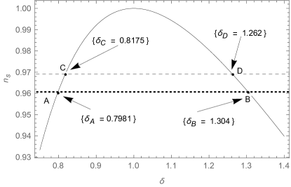
Figure 1: Plot between scalar spectral index $n_{s}$ and $\delta$. The straight dashed line shows an observational upper limit of the $n_{s}=0.9691$ and the straight dotted line is a lower limit of $n_{s}=0.9607$. In this paper, we do not consider the value of delta greater than one, therefore the value of $\delta$ must lie between $\delta_{A}\leq\delta\leq\delta_{C}$. As $\delta$ increases from $0.8175$, the value of $n_{s}$ crosses its upper limit.

After putting the value of $\varepsilon_{3}$ from the equation (60) in (58), we obtain the tensor-to-scalar ratio in the Jordan frame

$$r=\dfrac{48(1-\delta)^{2}}{(1+2\delta)^{2}}.$$ (63)

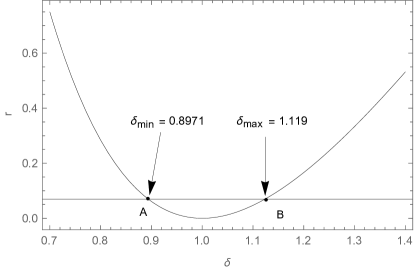
Figure 2: Plot between tensor-to-scalar ratio $r$ and $\delta$ in the Jordan frame. The straight solid line is an upper limit of $r=0.065$. This is an observational constraint on the parameter $\delta$. Points A and B indicate the minimum and maximum value of $\delta$, implying that $\delta$ has a value $0.8971\leq\delta<1.119$, including $r_{min}=0$ at $\delta=1$.

We have also found the relation between $n_{s}$ and $r$ by using equations (62) and (63)

$$r\simeq-\dfrac{24\delta}{(1+2\delta)}(n_{s}-1).$$ (64)

This relation shows the dependence on the $\delta$ parameter.

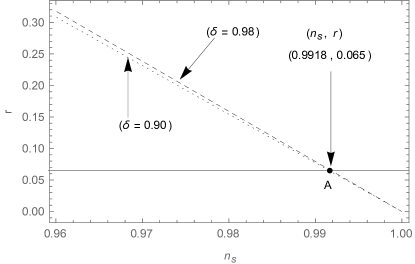
Figure 3: Plot between tensor-to-scalar ratio $r$ and scalar spectral index $n_{s}$ for $\delta=0.98$ and $\delta=0.90$ in the Jordan frame. The upper dashed line represents $\delta=0.98$ and the lower dotted line is drawn at $\delta=0.90$. The straight solid line is an upper bound on the value of $r$, which is $r<0.065$ coming from the observations. Point A denotes $n_{s}=0.9918$ at $r=0.065$.

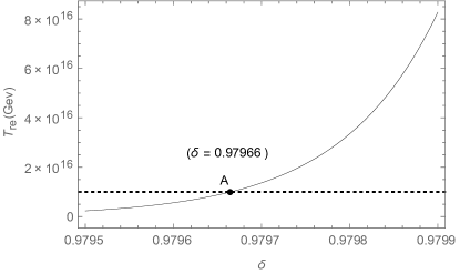
Figure 4: Plot between reheating temperature $T_{re}$ in $GeV$ and model parameter $\delta$ in the Jordan frame. The dotted straight line represents the lower limit of the $T_{re}=10^{16}$ GeV and intersects the curve at the point A $\delta=0.97966$.

We have used the relations (62) and (63) to obtain the plots of $\delta$ vs $n_{s}$ and $r$. It can be seen that both $n_{s}$ and $r$ depend only on the model parameter $\delta$. Fig.1 is a plot between $\delta$ and $n_{s}$, showing that the allowed values of the parameter $\delta$ are fixed by the observational upper and lower limit of the $n_{s}$. The range of the $\delta$ is $0.7981\leq\delta\leq 0.8175$. The value of the $n_{s}$ increases from 0.9607 to 0.9691 between the points A and C and decreases between the points D and B.

From Fig.1, we can see that initially $n_{s}$ increases with increasing $\delta$ and reaches the maximum at $\delta=1$ implying that there is no tilt in the CMB power spectrum.

Fig.2 is a plot between tensor-to-scalar ratio $r$ and $\delta$. We have a range of the $\delta$ parameter $0.8971\leq\delta\leq 1.1192$ obtained from the observational value of $r$. If the value of delta increases, the value of $r$ falls to zero before rising again. At $r=0$ with $\delta=1$, the primordial gravitational waves cannot be produced. As $r$ increases further from 0 to 0.065 with $\delta$ from 1 to 1.1192, having a gravitational wave component up to its uppermost observed value $r$ 0.065, even though this $\delta$ would imply a super inflation. Therefore, we can set the limit of the $\delta$ as $0.8971\leq\delta<1$ for inflation. However, this is inconsistent with the range of $\delta$ allowed in Fig.1. It can be seen that $r<0.1$ allows a better consistency of $r$ and $n_{s}$ with respect to their variation with $\delta$.

Therefore, it is interesting to check it further and so we plot tensor-to-scalar ratio $r$ and $n_{s}$ in Fig.3 with two different values of the model parameter $\delta$. Assuming $\delta\simeq 0.98$ gives a constraint on the value of $n_{s}$ and $r$. Both curves intersect at the point (0.9918, 0.065). However, while it is satisfactory for $r$, the value of $n_{s}$ is inconsistent with the observed range discussed in Fig.1. Again, consistency can be made stronger by allowing $r<0.1$ as shown in our model.

Reheating temperature may be determined in terms of $\delta$ after putting $N_{k}=60$, $\rho_{en}$, and $H_{k}$ from equations (49) and (59), respectively,

$$T_{re}=\Big{(}\frac{11g_{s,re}}{43}\Big{)}\Big{(}\dfrac{30}{\pi^{2}g_{re}}\Big{)}\Big{(}\frac{k}{a_{o}T_{o}}\Big{)}^{3}\Big{(}\dfrac{\sqrt{2}}{\pi\sqrt{\mathcal{P}_{s}}r}\Big{)}\dfrac{1}{\sqrt{F}}$$

$$\dfrac{3\delta(2+\delta)}{1+\delta}e^{3\sqrt{\frac{3}{2}}\frac{\delta}{1-\delta}}M_{p}.$$ (65)

Equation (65) depends on the model parameter and the observational parameters. By using equation (65) we can track the behaviour of reheating temperature $T_{re}$ with $\delta$. Thus, $T_{re}$ also sets a lower bound on $\delta$. From Fig.4, it can be seen that $T_{re}=10^{16}$ GeV sets this bound at $\delta=0.97966$. A lower reheating temperature would satisfy the observations of $r$ and $n_{s}$ and give a more consistent value of $\delta$.

IV Inflationary dynamics and reheating temperature in the Einstein frame

Replacing $f(R)$ by $[f(\chi)-f(\chi),_{\chi}(R-\chi)]$ in the equation (41) gives action as

$$\mathcal{A}=\dfrac{1}{2\kappa^{2}}\int{d^{4}x{\sqrt{-g}}[f(\chi)-f(\chi),_{\chi}(R-\chi))]},$$ (66)

where $\chi$ is an auxiliary field.

After defining $\varphi\equiv f(\chi),_{\chi}$ equation (66) can be written as

$$\mathcal{A}=\int{d^{4}x{\sqrt{-g}}\left[\dfrac{1}{2\kappa^{2}}\varphi R-U(\varphi)\right]},$$ (67)

where $U(\varphi)$ is potential of the field $(\varphi)$ as

$$U(\varphi)\equiv\dfrac{\chi(\varphi)\varphi-f(\chi(\varphi))}{2\kappa^{2}}.$$ (68)

We can rewrite the equation (41) as

$$\mathcal{A}=\int d^{4}x\sqrt{-g}\left(\frac{1}{2\kappa^{2}}f(R)R-U\right),$$ (69)

where

$$U=\dfrac{FR-f}{2\kappa^{2}}.$$ (70)

Invoking a conformal transformation of the metric tensor $\tilde{g}^{\mu\nu}=\Omega^{2}g^{\mu\nu}$ and $\sqrt{-g}=\Omega^{-4}\sqrt{-\tilde{g}}$, we obtain the action in the Einstein frame ($\mathcal{A}_{E}$) as

$$\mathcal{A}_{E}=\int d^{4}x\sqrt{-\tilde{g}}\left[\frac{1}{2\kappa^{2}}F\Omega^{-2}(\tilde{R}+6\tilde{\square}\omega-6\tilde{g}^{\mu\nu}\partial_{\mu}\omega\partial_{\nu}\omega)-\Omega^{-4}U\right],$$ (71)

where $\omega\equiv\ln\Omega$, $\partial_{\mu}\omega\equiv{\partial\omega}/{\partial\tilde{x}^{\mu}}$, $\tilde{\square}\omega\equiv({1}/{\sqrt{-g}})\partial_{\mu}(\sqrt{-\tilde{g}}\tilde{g}^{\mu\nu}\partial_{\nu}\omega)$,
$R=\Omega^{2}(\tilde{R}+6\tilde{\square}\omega-6\tilde{g}^{\mu\nu}\partial_{\mu}\omega\partial_{\nu}\omega)$.

We can rewrite the equation (71) by redefining the scalar field $\kappa\phi=\sqrt{3/2}\ln F$ and $\Omega^{2}=F$ in the Einstein frame as

$$\mathcal{A}_{E}=\int d^{4}x\sqrt{-\tilde{g}}\left[\frac{1}{2\kappa^{2}}\tilde{R}-\dfrac{1}{2}\tilde{g}^{\mu\nu}\partial_{\mu}\phi\partial_{\nu}\phi-V(\phi)\right]$$ (72)

where

$$V(\phi)=\dfrac{U}{F^{2}}=\dfrac{FR-f}{2\kappa^{2}F^{2}}.$$ (73)

Equation (72) shows that the scalar field $\phi$ is minimally coupled with the curvature. Since action (72) is same for the canonical single scalar field, therefore the dynamical equations and the conclusions drawn are equivalent in the Einstein frame for the slow roll inflation.

We have evaluated the potential of the scalar field $V(\phi)$ from the equation (73) by using the value of $R$, $f(R)$ and $F$ in term of the scalar field, $\phi$ as I20

$$V(\phi)=\dfrac{\delta R_{c}M_{p}^{2}}{2(1+\delta)^{\frac{1+\delta}{\delta}}}\left[e^{\sqrt{\frac{2}{3}}\frac{\phi}{M_{p}}}\right]^{\frac{1-\delta}{\delta}}.$$ (74)

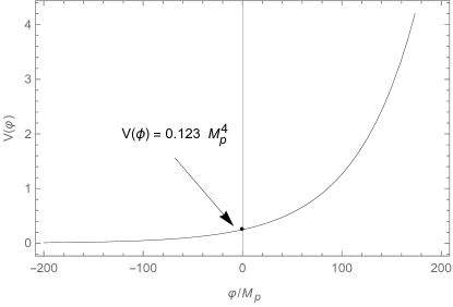
Figure 5: Plot showing the behavior of the scalar field potential $V(\phi)$ with respect to scalar field $\phi/M_{p}$. Here, we consider $\delta=0.98$ and $R_{c}=1$ in $M_{p}^{2}$ units. Homogeneous and isotropic scalar field potential has minimum if $\phi\rightarrow\infty$. Inflation begins at $\phi=M_{p}$ and rolling down towards $\phi=0$.

Interestingly, potentials of this type are able to produce slow roll inflation in the very early universe.

In Fig. 5, slow roll inflation ends as $\phi\rightarrow\infty$. Such a potential has a minima at $\infty$, therefore the scalar field (inflaton field) does not oscillate about minima. It goes on rolling towards infinity and decays into other particles in reheating phase. In this mechanism, potential has a global minima at the $\phi_{min}$ and the inflaton field oscillates about it. It may decay by a direct coupling to the matter field and other scalar field. Alternatively, reheating process may be followed by gravitational particle production VI1 ; Ia3 . However, in the present paper, we do not intend to discuss the process of the particle production during reheating.

Slow roll parameters in the scalar-tensor theory are defined by the equation (37) but in the Einstein frame $F=1$, and so $\tilde{\varepsilon}_{3}$ and $\tilde{\varepsilon}_{4}$ vanish Ia9 . Equation (37) becomes

$$\tilde{\varepsilon}_{1}\equiv-\dfrac{\dot{\tilde{H}}}{\tilde{H}^{2}}; \tilde{\varepsilon}_{2}\equiv\dfrac{\ddot{\phi}}{\tilde{H}\dot{\phi}}; \tilde{\varepsilon}_{3}=0; \tilde{\varepsilon}_{4}=0$$ (75)

where $\dot{\phi}={\partial\phi}/{\partial\tilde{t}}$ and $\ddot{\phi}={\partial^{2}\phi}/{\partial\tilde{t}^{2}}$, $d\tilde{t}=\sqrt{F}dt$, $\tilde{a}=\sqrt{F}a$ and the Hubble parameter $\tilde{H}\equiv(1/\tilde{a}){d\tilde{a}}/{d\tilde{t}}=({1}/\sqrt{F})\left(H+{\dot{F}}/{2F}\right)$.

There are two parameters $\tilde{\varepsilon}_{1}$ and $\tilde{\varepsilon}_{2}$ surviving in the Einstein frame. These can be expressed in terms of potential as well as in terms of $f(R)$ as III1

$$\tilde{\varepsilon}_{1}\equiv\dfrac{1}{2\kappa^{2}}\left(\dfrac{V,_{\phi}}{V}\right)^{2},$$ (76)

$$\tilde{\varepsilon}_{1}=\dfrac{1}{3}\left(\dfrac{2f-FR}{FR-f}\right)^{2},$$ (77)

$$\tilde{\varepsilon}_{2}=\dfrac{1}{2\kappa^{2}}\left(\dfrac{V,_{\phi}}{V}\right)^{2}-\dfrac{1}{\kappa^{2}}\left(\dfrac{V,_{\phi\phi}}{V}\right),$$ (78)

$$\tilde{\varepsilon}_{2}=\tilde{\varepsilon}_{1}-\eta,$$ (79)

where $\eta$ is given by the equation (11).

Further, $\eta$ can be expressed in terms of the $f(R)$ as III1

$$\eta=\dfrac{2}{3}\dfrac{F^{2}}{F^{\prime}(FR-f)}-\dfrac{2RF}{(FR-f)}+\dfrac{8}{3}$$ (80)

Using the slow roll condition (12) in the $\tilde{\rho}_{\phi}\simeq(1/2){\dot{\tilde{\phi}}}^{2}+V(\phi)$, the energy density of the scalar field becomes $\tilde{\rho}(\phi)\simeq V(\phi)$ while the Friedmann’s equation at the time of $k=\tilde{a}_{k}\tilde{H}_{k}$ turns out to be $\tilde{H}^{2}_{k}\simeq\tilde{\rho}_{k}(\phi)/3M_{p}^{2}$. At the end of the inflation, $(1/2)\dot{\phi}^{2}\simeq V(\phi)$ and the energy density $\tilde{\rho}_{en}(\phi)$ becomes

$$\tilde{\rho}_{en}(\phi)\simeq\dfrac{3}{2}V_{en}(\phi).$$ (81)

Inflaton potential at the end of inflation is

$$V_{en}(\phi)=V_{k}(\phi)e^{\sqrt{\frac{2}{3}}\Big{[}\frac{\phi_{k}}{M_{p}}-\frac{\phi_{en}}{M_{p}}\Big{]}\frac{1-\delta}{\delta}}.$$ (82)

Here, we have assumed that $\phi_{en}=0$; $\phi_{k}=M_{p}$ and $V(\phi)_{k}=3\tilde{H}^{2}_{k}M_{p}^{2}$. Putting these values in the above equation, we obtain

$$V_{en}(\phi)=3\tilde{H}^{2}_{k}M_{p}^{2}e^{\sqrt{\frac{2}{3}}\Big{(}\frac{\delta-1}{\delta}\Big{)}}.$$ (83)

Using the above value of the $V(\phi)_{en}$ in the (81), $\tilde{\rho}_{en}(\phi)$ becomes

$$\tilde{\rho}_{en}(\phi)\simeq\frac{9}{2}M_{p}^{2}\tilde{H}^{2}_{k}e^{\sqrt{\frac{2}{3}}\Big{(}\frac{\delta-1}{\delta}\Big{)}}.$$ (84)

In the Einstein frame, Hubble parameter in terms of $\tilde{\mathcal{P}}_{s}$ and $\tilde{r}$ is given as,

$$\tilde{H}_{k}=\Big{(}\dfrac{\pi M_{P}\sqrt{\tilde{\mathcal{P}}_{s}}\tilde{r}}{\sqrt{2}}\Big{)},$$ (85)

at the horizon exit.

Scalar spectral index $\tilde{n}_{s}$ in the Scalar-Tensor theory is given by the equation (39) Ib1 . Thus, using the values of $\tilde{\varepsilon}_{1}$, $\tilde{\varepsilon}_{2}$, $\tilde{\varepsilon}_{3}$ and $\tilde{\varepsilon}_{4}$ from the equation (75),

$$\tilde{n}_{s}-1\simeq-4\tilde{\varepsilon}_{1}-2\tilde{\varepsilon}_{2}.$$ (86)

which is further given as (from the equation (79))

$$\tilde{n}_{s}\simeq 1-6\tilde{\varepsilon}_{1}+2\eta.$$ (87)

Further, we have found the tensor-to-scalar ratio by putting the value of $Q_{s}={\dot{\phi}^{2}}/{\tilde{H}^{2}}$ in the equation (40) in the Einstein frame Ia9 as

$$\tilde{r}\simeq-16\frac{\dot{\tilde{H}}}{\tilde{H}^{2}}=16\tilde{\varepsilon}_{1}.$$ (88)

We can also determine the number of e-foldings in the Einstein frame from the equation (15) as

$$N=\int^{\phi_{60}}_{\phi_{end}}{\dfrac{d(\phi/M_{p})}{\sqrt{2\tilde{\varepsilon}_{1}}}}.$$ (89)

This expression is further used to calculate the value of the $\delta$ parameter.

IV.1 Scalar spectral index, tensor-to-scalar ratio and reheating temperature in the Einstein frame in the $f(R)={R^{1+\delta}}/{R^{\delta}_{c}}$ model.

In this section we calculate $\tilde{\varepsilon}_{1}$ and $\eta$ in the model (1) by using the equation (77) and (80), respectively, as

$$\tilde{\varepsilon}_{1}=\dfrac{1}{3}\dfrac{(1-\delta)^{2}}{\delta^{2}}$$ (90)

and

$$\eta=\dfrac{2(1-\delta)^{2}}{3\delta^{2}}=2\tilde{\varepsilon}_{1}.$$ (91)

These expressions show dependence on the single parameter $\delta$ only, and thus are sensitive to the $f(R)$ model parameter.

This leads us to obtain the expressions for scalar spectral index $\tilde{n}_{s}$ and tensor-to-scalar ratio $\tilde{r}$ using the value of $\tilde{\varepsilon}_{1}$ and $\eta$ in the equation (87) and (88), respectively, as

$$\tilde{n}_{s}\simeq 1-\dfrac{2}{3}\left(\dfrac{1-\delta}{\delta}\right)^{2},$$ (92)

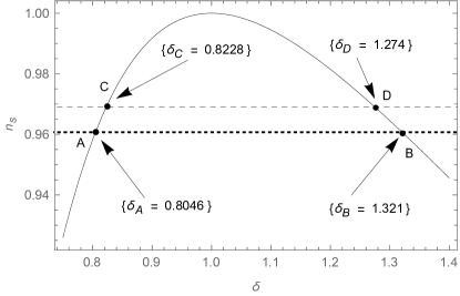
Figure 6: Plot between scalar spectral index $\tilde{n}_{s}$ and $\delta$ parameter in the Einstein frame. The dashed straight line is the upper limit of the $\tilde{n}_{s}=0.9691$ and dotted straight line is the lower limit $\tilde{n}_{s}=0.9607$. The value of $\delta$ lies over the range $0.8046\leq\delta\leq 0.8228$. The variation also shows a maximum at $\delta=1$ and $\tilde{n}_{s}=1$.

$$\tilde{r}=\dfrac{16}{3}\dfrac{(1-\delta)^{2}}{\delta^{2}}.$$ (93)

Using equations (92) and (93), we get the relation between spectral index and tensor-to-scalar ratio as

$$\tilde{r}=-8(\tilde{n}_{s}-1).$$ (94)

It may be noticed that the above relation is independent of $\delta$ parameter.

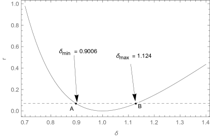
Figure 7: Plot between tensor-to-scalar ratio $\tilde{r}$ and $\delta$ in the Einstein frame. The dashed straight line at $\tilde{r}=0.065$ sets the observational limit on the $\delta$ parameter. It marks a minimum at $\delta=1$ with $r_{min}=0$.

Further, we calculate the value of $\delta$ from the number of e-foldings by putting the value of $\tilde{\varepsilon}_{1}$ in the equation (89),

$$N=\int^{\phi_{60}}_{\phi_{end}}{\dfrac{d(\phi/M_{p})}{\sqrt{2(1-\delta)^{2}/3\delta^{2}}}}.$$ (95)

Integrating equation (95),

$$N=\sqrt{\dfrac{3}{2}}\dfrac{\delta}{(1-\delta)}\left[\dfrac{\phi_{60}}{M_{p}}-\dfrac{\phi_{end}}{M_{p}}\right].$$ (96)

If we assume that inflation starts at $\phi_{60}=M_{p}$ and ends at $\phi_{end}=0$, then from equation (96) we have

$$N=\sqrt{\dfrac{3}{2}}\dfrac{\delta}{(1-\delta)}$$ (97)

We have kept the number of e-folds $N=60$ with a view to solve the horizon problem and flatness problem in the $\Lambda$CDM model. Putting the value of $N$ in the equation (97) we can constrain our model parameter. Thus,

$$\dfrac{\delta}{(1-\delta)}=60\sqrt{\dfrac{2}{3}}$$ (98)

$$\delta=0.97999\simeq 0.98$$ (99)

which is very close to 1. It is particularly significant because using the value of $\delta$, we are able to calculate the scalar spectral index and tensor-to-scalar ratio, both in the Jordan frame and the Einstein frame.

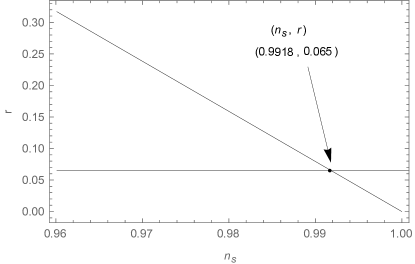
Figure 8: Plot between tensor-to-scalar ratio $\tilde{r}$ and scalar spectral index $\tilde{n}_{s}$ for $\delta=0.98$ in the Einstein frame. The horizontal straight line is an upper bound on the $\tilde{r}$. At the point of intersection A, the value of $\tilde{n}_{s}$ is $0.9918$.

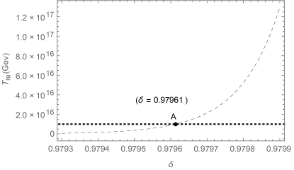
Figure 9: Plot between the reheating temperature $T_{re}$ and the model parameter $\delta$ in the Einstein frame. The straight dotted line provides a lower bound on the reheating temperature giving $\delta=0.97961.$

The equation (92) gives the relation between $n_{s}$ and $\delta$ also seen in Fig.6, where we have constrained the value of $\delta$ parameter from the observational upper and lower limits of the $n_{s}$. The admissible range is $0.8046\leq\delta\leq 0.8228$. The solid curve has a maximum at the value of $\tilde{n}_{s}=1$ and $\delta=1$ which implies that there is no tilt in the power spectrum of the CMB.

In Fig.7, we have shown a range of the parameter $0.9006\leq\delta\leq 1.124$ from the observational value of $\tilde{r}$. If the value of delta increases then the $\tilde{r}$ goes towards the zero before increasing with $\delta$. The value of $\tilde{r}$ is zero at $\delta=1$, which means that the primordial gravitational waves can not be produced during inflation but metric fluctuations must present in the early universe. Since an increasing value of $\delta$ makes $\tilde{r}$ become greater than 0.065, therefore, we can set the optimal bound on the $\delta$ as $0.9006\leq\delta<1$ for inflation.

Indeed, if we satisfy $r<0.065$ then $\tilde{n}_{s}$ must be at least equal to $0.9918$, which can be further relaxed if $r<0.1$. This behaviour can be seen from Fig.8.

With the above analysis, we can comment that although there is a lack of complete concordance range of the $\delta$ parameter from the Fig.6 and Fig.7, however, from the Fig.3 and Fig.8, we have obtained the values of $n_{s}\leq 0.9918$ with our model parameter $\delta=0.98$. Therefore, we may conclude that $\delta$ lies in the range $0.8046\leq\delta\leq 1$ in the Einstein frame.

Now, the reheating temperature from (32) given in the Einstein frame after putting the value of $\tilde{N}_{k}$, $\tilde{H}_{k}$ and $\tilde{\rho}_{\phi}(en)$ from equations (97), (85) and (84), respectively, into (89) becomes as

$$\tilde{T}_{re}=\frac{9}{2}\Big{(}\frac{11g_{s,re}}{43}\Big{)}\Big{(}\dfrac{30}{\pi^{2}g_{re}}\Big{)}\Big{(}\frac{k}{a_{o}T_{o}}\Big{)}^{3}\Big{(}\dfrac{\sqrt{2}}{\pi\sqrt{\tilde{\mathcal{P}}_{s}}\tilde{r}}\Big{)}$$

$$e^{\sqrt{\frac{3}{2}}\frac{\delta-1}{\delta}}e^{3\sqrt{\frac{2}{3}}\frac{\delta}{1-\delta}}M_{p}.$$ (100)

The behaviour of $\tilde{T}_{re}$ from (100) with respect to $\delta$ can be seen in the Fig.9, where $\tilde{T}_{re}=10^{16}$ GeV is a lower bound indicating $\delta=0.97961$. This provides the minimum energy required to decouple gravitational field from other fields.

V Are the Jordan frame and the Einstein frame equivalent?

In the foregoing discussion, we have seen conformal equivalence with the help of $n_{s}$, $r$ and $T_{re}$ between the Jordan and the Einstein frame in the very early universe. In the Jordan frame, we obtained scalar spectral index and tensor-to-scalar ratio, respectively, as

$$n_{s}=1-\dfrac{2}{\delta}\dfrac{(1-\delta)^{2}}{(1+2\delta)}; r=48\dfrac{(1-\delta)^{2}}{(1+2\delta)^{2}},$$ (101)

and in the Einstein frame as

$$\tilde{n}_{s}=1-\dfrac{2}{3}\dfrac{(1-\delta)^{2}}{\delta^{2}}; \tilde{r}=\dfrac{16}{3}\dfrac{(1-\delta)^{2}}{\delta^{2}}.$$ (102)

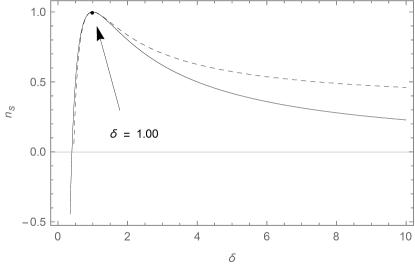
Figure 10: Plot between scalar spectral index $n_{s}$ and $\delta$ in the Jordan frame (solid curve) and the Einstein frame (dashed curve). As $\delta$ rises above $\delta=1$, we observe a marked difference between the two frames, while below $\delta=1$ they are approximately indistinguishable from each other.

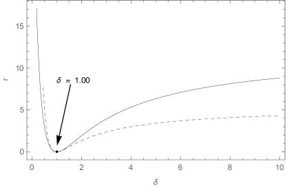
Figure 11: Plot between tensor-to-scalar ratio $r$ and $\delta$ in the Jordan frame (solid curve) and the Einstein frame (dashed curve).

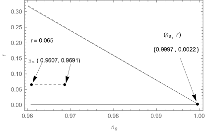
Figure 12: Plot between tensor-to-scalar ratio $r$ and scalar spectral index $n_{s}$ at $\delta=0.98$ in the Jordan frame (solid curve) and the Einstein frame (dashed curve). The horizontal dashed line provides an observational limit on $n_{s}$ at $r=0.065$, whereas the lower solid horizontal straight line is drawn by using the calculated value of $r=0.0022$.

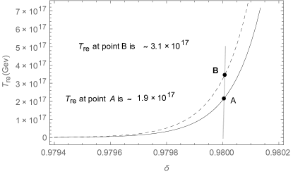
Figure 13: Plot between reheating temperature $T_{re}$ and the model parameter $\delta$ in the Jordan frame and the Einstein frame. The value of the reheating temperatures are approximately same.

We may compare this to the Starobinsky model, $f(R)=R+R^{2}/6M^{2}$, where the spectral index and tensor-to-scalar ratio in the Jordan frame are Ia5 ; Ia9

$$n_{s}\simeq 1-\dfrac{2}{N_{k}}; r\simeq\dfrac{12}{N_{k}^{2}},$$ (103)

with ${N}_{k}\simeq{1}/(2{\varepsilon_{1}})$, and in the Einstein frame

$$\tilde{n_{s}}\simeq 1-\dfrac{2}{\tilde{N}_{k}}-\dfrac{3}{\tilde{N}_{k}^{2}}; \tilde{r}\simeq\dfrac{12}{\tilde{N}_{k}^{2}},$$ (104)

with $\tilde{N}_{k}={1}/(2\tilde{\varepsilon_{1}})$.

The above equations (103) and (104) clearly show that the expressions for spectral index and tensor-to-scalar ratio in the Jordan frame and in the Einstein frame, respectively, are not exactly same. However, as the third term containing $3/(\tilde{N}_{k}^{2})$ in the equation (104) is negligible in comparison to the second term $1/{\tilde{N}_{k}}$, equations (103) and (104) become approximately equivalent in the Starobinski model.

Similarly, for our model (1), spectral index and tensor-to-scalar ratio in the Jordan frame and in the Einstein frame are exactly same if $\delta\simeq 1$. However, we use $\delta=0.98$ from equation (99) for calculating scalar spectral index and tensor-to-scalar ratio in the Jordan frame and in the Einstein frame. The corresponding values turn out, respectively, as

$$n_{s}=0.99972; r=2.2\times 10^{-3},$$ (105)

$$\tilde{n}_{s}=0.99972 \tilde{r}=2.19\times 10^{-3}.$$ (106)

Thus, we find that the Jordan and the Einstein frame are equivalent when $\delta=0.98$ as seen from equations (105) and (106). A comparison between both frames is shown in Figures 10, 11, 12, 13. There is an increasingly marked departure from mutual equivalence as the value of $\delta$ rises above $\delta=1$ during the inflation. On the contrary, from Fig.10 and Fig.11, we note that when $\delta$ falls below $\delta=1$, the differences in the values of $n_{s}$ and $r$ in the Jordan frame and in the Einstein frame are quite small making the two frames almost indistinguishable from each other.

In Fig.12, the maximum and minimum observational values of $n_{s}$ at $r=0.065$ have been shown by the horizontal dashed straight line. The solid straight line at the bottom represents the calculated value of $r\simeq 0.0022$ indicating $n_{s}=0.9997$ in the both frames. The difference between the calculated value ($n_{s}=0.9997$ at $\delta=0.98$) and the observational value ($n_{s}=0.9649\pm 0.0042$) lies over the range $\sim 0.0306$ to $0.0390$.

Further, we have the value of reheating temperature at $\delta=0.98$ in the Jordan frame and in the Einstein frame, respectively, as

$$T_{re}=4.42M_{p}\Big{(}\frac{11g_{s,re}}{43}\Big{)}\Big{(}\dfrac{30}{\pi^{2}g_{re}}\Big{)}\Big{(}\frac{k}{a_{o}T_{o}}\Big{)}^{3}$$

$$\Big{(}\dfrac{\sqrt{2}}{\pi\sqrt{\mathcal{P}_{s}}r}\Big{)}e^{3N_{k}}\dfrac{1}{\sqrt{F}},$$ (107)

and

$$\tilde{T}_{re}=4.57M_{p}\Big{(}\frac{11g_{s,re}}{43}\Big{)}\Big{(}\dfrac{30}{\pi^{2}g_{re}}\Big{)}$$

$$\Big{(}\frac{k}{a_{o}T_{o}}\Big{)}^{3}\Big{(}\dfrac{\sqrt{2}}{\pi\sqrt{\tilde{\mathcal{P}}_{s}}\tilde{r}}\Big{)}e^{3\tilde{N}_{k}}.$$ (108)

Now, putting ${F}=exp(\sqrt{(2/3)}\phi/M_{p})$ in equation (32) where $\phi=M_{p}$ when the inflation begins and $\phi\leq M_{p}$ at the time of horizon exit, we obtain $\tilde{T}_{re}$ in the Einstein frame through

$$T_{re}\simeq\frac{1}{\sqrt{F}}\tilde{T}_{re}.$$ (109)

The above equation (109) shows the relation between reheating temperature in the Jordan frame and in the Einstein frame. In both cases, $\sqrt{F}\ll 1$ or $\sqrt{F}\gg 1$, these frames do not remain equivalent. ${T}_{re}$ and $\tilde{T}_{re}$ strongly depend on the number of e-folding and energy density at the end of the inflation.

Numerical values of reheating temperature at $\delta=0.98$ in the Jordan frame and the Einstein frame are given as

$${T}_{re}=1.98\times 10^{17}GeV; \tilde{T}_{re}=3.1\times 10^{17}GeV,$$ (110)

and at $\delta\simeq 0.9789$ (or number of e-folding $N\simeq 57$),

$${T}_{re}=2.3\times 10^{13}GeV; \tilde{T}_{re}=3.7\times 10^{13}GeV.$$ (111)

At $\delta\simeq 0.9788$

$${T}_{re}=5.99\times 10^{12}GeV; \tilde{T}_{re}=9.3\times 10^{12}GeV.$$ (112)

We can see from the equations (110), (111) and (112) that even a small variation in the value of $\delta$ produces a drastic change in the reheating temperature $T_{re}$. However, both frames provide approximately same value of reheating temperature.

Equations (105), (106), (110), (111) and (112), are approximately same as a consequence of equivalence between the Jordan frame and the Einstein frame. This is also seen from Fig.13, where the curves show the similar behaviour leaving only a small difference in the value of reheating temperature.

VI Conclusion

We have ended up this paper showing equivalence between the Jordan frame and the Einstein frame, while examining the viability of our model. We calculated the model parameter $\delta$ during the inflation and attempted to constraint the upper limit on the reheating temperature. Throughout, we have studied the framework of $f(R)=R^{1+\delta}/R_{c}^{\delta}$ model which provides the value of the power spectrum indices very close to the observations. Inflationary slow roll parameters, scalar spectral indices and tensor-to-scalar ratio are sensitive to $\delta$ parameter. If $\delta=1$ then $n_{s}$ becomes $=1$ implying that tilt of the power spectrum is zero. However, considering that the Hubble parameter is not exactly constant during inflation, tilt should be $n_{s}\sim 1$. We have calculated value $n_{s}=0.99972$ at $\delta=0.98$ but the observational constraints on the scalar spectral index from Planck 2018 give $n_{s}=0.9647\pm 0.0042$. Thus, there is small difference between the observed and the calculated value of the $n_{s}$ in our model, that can be attributed to several factors, including statistical or systematic errors. We also see that tensor-to-scalar ratio $r$ becomes zero if $\delta=1$ which means that the amplitude of the tensor power spectrum is zero. Therefore, primordial gravitational waves cannot not get produced during inflation if $\delta=1$, and $\delta\simeq 0.98$ appears consistent with inflation.

We have the relation (64) between $n_{s}$ and $r$ in the Jordan frame in terms of $\delta$ parameter, while on the other hand, the relation (94) is completely independent of $\delta$ in the Einstein frame. Thus, it leads to the same result as equation (64) at $\delta=0.98$. This can also be seen from the Fig.12. Above all, it appears that $\delta=0.98$ is the most preferred value of $\delta$ during the inflation for our model.

We have obtained another result about $\delta$ parameter which shows that the Jordan and the Einstein frame are equivalent if $\delta=0.98$. In addition, we found that scalar spectral index, tensor-to-scalar ratio and reheating temperature in the Jordan frame show an increasingly marked difference from the Einstein frame when $\delta$ rises above $\delta=1$. Thus, a lower value of this model parameter is favoured.

Calculations show that the reheating temperature at $\delta=0.98$ is $T_{re}\sim 10^{17}$ GeV. This value of the reheating temperature is required for grand unification symmetry breaking. However, it is interesting to see that if we introduce even a small variation from $\delta=0.98$ to $\delta=0.9788$, then the reheating temperature hugely drops to $T_{re}\sim 10^{13}$ GeV. Clearly, this shows that the reheating temperature is strongly sensitive to the value of $\delta$ parameter, although it does not tell us how exactly reheating occurs. In our future work, we will attempt to calculate reheating temperature via perturbative reheating mechanism or other possible processes for such potential. Further investigations may be done to study phase transition and we guess that some corrections may arise in the potential. We would also use this model to examine the evolution of $\delta$, especially up to phase of the late-time cosmic acceleration of the universe.

Acknowledgments

Authors are thankful to IUCAA, Pune for extending the facilities and support under the associateship programme where most of the work was done. AS also thanks Vipin Sharma, Bal Krishna Yadav, Swagat Mishra and Varun Sahni for the useful discussions on various aspects of inflationary theories.

References

- (1) A. A. Starobinsky, “A new type of isotropic cosmological models without singularity”, Phys. Lett. B 91, 99, (1980).
- (2) A. D. Linde, “Is the cosmological constant really a constant?”, JETP Lett. 19,183, (1974). [Pisma Zh. Eksp. Teor. Fiz. 19 (1974) 320].
- (3) M. M. Verma, “Dark energy as a manifestation of the non-constant cosmological constant”, Astrophys. Space Sci. 330, 101 (2010).
- (4) A. D. Linde, “Phase transitions in gauge theories and cosmology”, Rept. Prog. Phys. 42, 389 (1979).
- (5) A. H. Guth, “The inflationary universe: A possible solution to the horizon and flatness problems”, Phys. Rev. D 23, 347 (1981).
- (6) D. A. Kirzhnits and A. D. Linde, “Symmetry behavior in gauge theories”, Ann. Phys. 101, 195 (1976).
- (7) E. W. Kolb and M. S. Turner, “The early universe”, Taylor and Francis (CRC Press) (2019).
- (8) J. V. Narlikar, “An introduction to cosmoslogy”, Cambridge University Press, Third Edition (2017).
- (9) A. D. Linde, “A new inflationary universe scenario: A possible solution of the horizon, flatness, homogeneity, isotropy and primordial monopole problems”, Phys. Lett. B 108, 389 (1982).
- (10) A. A. Penzias and R. W. Wilson, “A measurement of excess antenna temperature at 4080 Mc/s.”, Astrophys. J. 142, 419, (1965).
- (11) N. W. Boggess et al., “The COBE mission: Its design and performance two years after launch”, Astrophys. J 397, 420 (1992).
- (12) A. D. Linde, “Chaotic inflation”, Phys. Lett. B 129, 177 (1983).
- (13) A. D. Linde, “Inflationary cosmology”, Lect. Notes Phys. 738,1 (2008).
- (14) D. S. Gorbunov and V. A. Rubakov, “Introduction to the theory of the early universe: Cosmological perturbations and inflationary theory”, Hackensack, USA: World Scientific 489 p (2011).
- (15) D. H. Lyth and A. Riotto, “Particle physics models of inflation and the cosmological density perturbation”, Phys. Rept. 314, 1 (1999).
- (16) S. Capozziello, “Curvature quintessence”, Int. J. Mod. Phys. D, 11, 483, (2002).
- (17) F. L. Bezrukov and M. Shaposhnikov, “The Standard model Higgs boson as the inflaton”, Phys. Lett. B 659, 703 (2008).
- (18) Planck Collaboration, Y. Akrami et al., “Planck 2018 results. X. Constraints on inflation”, arXiv:1807.06211.
- (19) A. A. Starobinsky, “Disappearing cosmological constant in gravity”, JETP Lett. 86, 157 (2007).
- (20) S. A. Appleby and R. A. Battye, “Do consistent models mimic general relativity plus ?”, Phys. Lett. B 654, 7 (2007).
- (21) E. V. Linder, “Exponential gravity”, Phys. Rev. D 80, 123528 (2009).
- (22) W. Hu and I. Sawicki, “Models of cosmic acceleration that evade solar system tests”, Phys. Rev. D 76, 064004 (2007).
- (23) C. Brans, and R.H. Dicke, “Mach’s Principle and a Relativistic Theory of Gravitation”, Phys. Rev. 124, 925, (1961).
- (24) V. Faraoni and E. Gunzig, “ Einstein frame or Jordan frame?”, Int. J. Theor. Phys. 38, 217, (1999).
- (25) F. Bezrukov and M. Shaposhnikov, “Standard model Higgs boson mass from inflation: Two loop analysis”, J. High Energy Phys. 07, 089 (2009).
- (26) J. White, M. Minamitsuji and M. Sasaki, “Curvature perturbation in multi-field inflation with non-minimal coupling”, J. Cosmol. Astropart. Phys. 1207, 039 (2012).
- (27) S. Bahamonde, S. D. Odintsov, V. K. Oikonomou and P. V. Tretyakov, “Deceleration versus Acceleration Universe in Different Frames of Gravity”, Phys. Lett. B 766, 225 (2017).
- (28) D. Nandi, “Stable contraction in Brans-Dicke cosmology”, J. Cosmol. Astropart. Phys. 1905, 040 (2018); D. Nandi, “Note on stability in conformally connected frames”, Phys. Rev. D99, 103532 (2019).
- (29) B. K. Yadav and M. M. Verma, “Dark matter as scalaron in gravity models”, J. Cosmol. Astropart. Phys. 10, 052 (2019).
- (30) C. G. Boehmer, T. Harko and F. S. N. Lobo, “Dark matter as a geometric effect in gravity”, Astropart. Phys. 29, 386 (2008).
- (31) V. K. Sharma, B. K. Yadav and M. M. Verma, “Extended galactic rotational velocity profiles in gravity background”, Eur. Phys. J. C 80, 619 (2020).
- (32) S. Perlmutter, S. Gabi, G. Goldhaber, A. Goobar, D.E. Groom, et al., “Measurements of the cosmological parameters and from the first seven supernovae at z 0.35”, Astrophys. J. 483, 565 (1997).
- (33) A. G. Riess, A. V. Filippenko, P. Challis, A. Clocchiatti, A. Diercks, et al., “Observational evidence from supernovae for an accelerating universe and a cosmological constant”, Astron. J. 116, 1009, (1998).
- (34) L. Amendola and S. Tsujikawa, “Dark energy: Theory and observations”, Cambridge University Press, First Edition, (2010).
- (35) V. Mukhanov, “Physical foundations of cosmology”, Cambridge University Press, UK (2005).
- (36) S. Nojiri, S. D. Odintsov and V. K. Oikonomou, “Modified gravity theories in a nutshell: Inflation, bounce and late-time evolution”, Phys. Rep. 692, 1 (2017).
- (37) D. H. Lyth, “Particle physics models of inflation”, Lect. Notes Phys. 738, 81 (2008); A. R. Liddle and D. H. Lyth, “Cosmological inflation and large-scale structure”, Cambridge University Press, UK, First Publication (2000).
- (38) S. M. Caroll, “Spacetime and geometry: An introduction to general relativity”, Pearson Education, First Edition, (2016).
- (39) M. Amin, S. Khalil and M. Salah, “A viable logarithmic model for inflation”, J. Cosmol. Astropart. Phys. 08, 043 (2016).
- (40) A. de Felice and S. Tsujikawa, “ theories”, Living Rev. Relativ., 13, 3 (2010).
- (41) P. A. R. Ade et al. (BICEP2 and Keck Array Collaborations), “BICEP2 / Keck Array x: Constraints on Primordial Gravitational Waves using Planck, WMAP, and New BICEP2/Keck Observations through the 2015 Season”, Phys. Rev. Lett. 121, 221301 (2018).
- (42) J. C. Hwang, and H. Noh, “Cosmological perturbations in generalized gravity theories”, Phys. Rev. D 54, 1460 (1996).
- (43) V. K. Oikonomou, “Exponential inflation with gravity”, Phys. Rev D 97, 064001 (2018).
- (44) T. Miranda, C. Escamilla-Rivera, O. F. Piattella and J. C. Fabris, “Genric slow-roll and non-gaussianity parameters in theories”, J. Cosmol. Astropart. Phys. 05, 028 (2019).
- (45) Y. Akrami, R. Kallosh, A. Linde and V. Vardanyan, “The landscape, the swampland and the era of precision”, Fortsch. Phys. 67, 1800075 (2019).
- (46) E. J. Copeland, N. J. Nunes, and F. Rosati, “Quintessence models in supergravity”, Phys. Rev. D 62, 123503 (2000).