Template Matching and Change Point Detection by M-estimation

Abstract

We consider the fundamental problem of matching a template to a signal. We do so by M-estimation, which encompasses procedures that are robust to gross errors (i.e., outliers). Using standard results from empirical process theory, we derive the convergence rate and the asymptotic distribution of the M-estimator under relatively mild assumptions. We also discuss the optimality of the estimator, both in finite samples in the minimax sense and in the large-sample limit in terms of local minimaxity and relative efficiency. Although most of the paper is dedicated to the study of the basic shift model in the context of a random design, we consider many extensions towards the end of the paper, including more flexible templates, fixed designs, the agnostic setting, and more.

1 Introduction

A basic task in signal processing is the matching of a template, aka filter or pattern, to a noisy signal (Brunelli, 2009; Turin, 1960). There has been an extensive amount of research is this very broad area, as applications are many, from locating blood vessels and tumors in medical imaging to more sophisticated tasks such as locating a human face or ‘recognizing’ objects like cars in images (Hjelmås and Low, 2001; Belongie et al., 2002; Lowe, 1999; Serre et al., 2005).

Scan statistic

In statistics, this template matching problem has been considered in different variants. Such is the literature on the scan statistic (Glaz and Balakrishnan, 2012; Glaz et al., 2009, 2001), where the focus has been on the detection of the presence of the filter somewhere in the noisy signal, rather than the estimation of its location (when present), for which theory has been developed, including first-order performance bounds (Walther, 2010; Desolneux et al., 2003; Arias-Castro et al., 2005; Arias-Castro et al., 2011, 2018) with a minimax decision theory perspective, as well as more refined results studying and even establishing the limit distribution (Naus and Wallenstein, 2004; Pozdnyakov et al., 2005; Glaz and Zhang, 2004; Wang and Glaz, 2014; Haiman and Preda, 2006; Proksch et al., 2018; König et al., 2020; Sharpnack and Arias-Castro, 2016). Some of this has some nontrivial intersections with the study of the maximum of various types of random walks and similar processes (Shao, 1995; Jiang, 2002; Boutsikas and Koutras, 2006; Siegmund and Venkatraman, 1995; Kabluchko, 2011). In this literature, there are comparatively very few papers that tackle the problem of estimating the location of the template: Jeng et al. (2010) establish a consistency result for the location of very short intervals, while Kou (2017) shows that the scan statistic is, as a location estimator, consistent near the signal-to-noise ratio required for mere detection.

Change point detection

Discontinuities are features of great importance in practice, and it is no coincidence that the template that is most often considered in the scan statistic literature is the indicator of an interval — or multiple intervals as in (Jeng et al., 2010; Hall and Jin, 2010; Frick et al., 2014) — or a rectangle or other shape as in (Arias-Castro et al., 2011; Walther, 2010). A discontinuity is sometimes called a change point, and there is also a large body of work in that area. While some of the work on change point detection happens under the umbrella of sequential analysis where data are streaming in (Siegmund, 2013), what we are discussing here is most closely related to the ‘offline’ or ‘a posteriori’ setting where all data are readily available (Truong et al., 2020). This spans, in itself, a very large literature (Chen and Gupta, 2011; Csörgö and Horváth, 1997; Brodsky and Darkhovsky, 2013; Basseville and Nikiforov, 1993). First-order performance bounds are available, for example in (Frick et al., 2014; He and Severini, 2010), but distributional limits are more scarce, at least when it comes to the location of the discontinuities. Hinkley (1970) derives the asymptotic distribution of the maximum likelihood ratio when everything else about the model is known. Yao and Au (1989) obtain the asymptotic distribution of the least squares estimator of a piecewise constant signal, and this is extended to other U-type statistics in (Döring, 2011; Mauer, 2018; Ferger, 2001; Bai, 1997). (Ferger, 1994; Dümbgen, 1991) consider estimating the location of a change of distribution in a sequence of random variables. We note that all this work is done in the context of a deterministic design corresponding to a regular grid (as in a signal processing setting).

Alignment

The problem of matching a (clean/noiseless) template to a signal is closely related to the problem of matching two or more noisy signals, sometimes referred to as aligning or registering or synchronizing the signals. While this literature is also very large on the side of methodology and applications (Zitova and Flusser, 2003; Hajnal and Hill, 2001; Sotiras et al., 2013), there is a sizable literature that develops theory for such problems. Some of these theoretical developments were made in the context of functional data, which is where in statistics such problems are most prominent, and where the problem is sometimes called ‘self-modeling’ or ‘shape invariant modeling’ (Lawton et al., 1972). In this context, consistency results and/or rates of convergence are obtained in (Kneip and Gasser, 1988, 1992; Wang and Gasser, 1999), while distributional limits are derived in (Härdle and Marron, 1990; Gamboa et al., 2007; Bigot et al., 2009; Trigano et al., 2011; Kneip and Engel, 1995), and also in (Vimond, 2010), where questions of efficiency are considered in a semi-parametric model were only smoothness assumptions are made on the common ‘shape’. Collier and Dalalyan (2012, 2015) consider a hypothesis testing problem in that setting. We note that the signals are typically smoothed before the alignment is carried out, and that the Fourier transform plays an important role, and the noise is often assumed to be Gaussian or to have sub-Gaussian tails. This is in contrast to the present setting in which no smoothing is used and the Fourier transform plays no role, and we work with minimal assumptions on the noise distribution. We mention a more recent line of work on this problem which focuses on more complex and noisy settings arising in applications such as cryo-electron microscopy (Perry et al., 2019; Wang and Singer, 2013; Perry et al., 2018).

Contribution

In the present paper we study a standard mathematical model for matching a template to a noisy signal by M-estimation. While the most popular method may still be based on maximizing the (Pearson) correlation, the estimators we study can be made much more robust to heavy-tailed noise or the presence of outlying observations. We draw on standard empirical process theory and decision theory, as expounded in (van der Vaart, 1998), to derive limit distributions and minimax convergence rates in a wide array of situations.

1.1 Model

We assume a regression model with additive error

$$Y_{i}=f(X_{i}-\theta^{*})+Z_{i},\quad i=1,\dots,n,$$ (1)

where $f:\mathbb{R}\to\mathbb{R}$ is a known function referred to as the template, and $\theta^{*}\in\mathbb{R}$ is the unknown shift of interest. The design points $X_{1},\dots,X_{n}$ are assumed to be iid with density $\lambda$. The noise or measurement error variables $Z_{1},\dots,Z_{n}$ are assumed iid with density $\phi$, and independent of the design points. Note that in this model $(X_{1},Y_{1}),\dots,(X_{n},Y_{n})$ independent and identically distributed.

Assumption 1.

We assume everywhere that $f$ is compactly supported and, for convenience, càdlag with none or finitely many discontinuities. In particular, $f$ is bounded. And to make sure the shift parameter is identifiable, we also assume that, for any $\theta\neq\theta^{*}$, $f(\cdot-\theta)\neq f(\cdot-\theta^{*})$ on a set of positive measure under $\lambda$, or equivalently, $\int(f(x-\theta^{*})-f(x-\theta))^{2}\lambda(x){\rm d}x>0$ whenever $\theta\neq\theta^{*}$.

Assumption 2.

We assume everywhere that $\lambda$ is compactly supported.

Assumption 3.

We assume everywhere that $\phi$ is even, so that the noise is symmetric about 0.

The assumption that the template and the design density both have compact support is for convenience — although it already applies in most of the settings encountered in practice. It allows us to effectively restrict the parameter space to a compact interval of the real line. Indeed, take $A$ large enough that $f$ and $\lambda$ are both supported on $[-A,A]$. Then the model (1) is effectively parameterized by $\theta\in[-2A,2A]$ as the model is the same, namely $Y_{i}=Z_{i}$, whenever $\theta$ is outside that interval. The assumption that the noise is symmetric is not needed everywhere, but already covers interesting situations.

1.2 Goal and methods

Our goal is, in signal processing terminology, to match the template $f$ to the signal $Y$, which in statistical terms consists in the estimation of the shift $\theta^{*}$. We consider an M-estimator defined implicitly as the solution to the following optimization problem

$$\hat{\theta}:=\operatorname*{arg\,min}_{\theta}\sum_{i=1}^{n}{\sf L}(Y_{i}-f(X_{i}-\theta)),$$ (2)

where ${\sf L}$ is a loss function chosen by the analyst. A popular choice is the squared error loss, ${\sf L}(y)=y^{2}$, which defines the least squares estimator

$$\hat{\theta}:=\operatorname*{arg\,min}_{\theta}\sum_{i=1}^{n}(Y_{i}-f(X_{i}-\theta))^{2}.$$ (3)

This is the maximum likelihood estimator when the noise distribution is Gaussian. Another popular choice is the absolute-value loss, ${\sf L}(y)=|y|$, which defines the least absolute-value estimator

$$\hat{\theta}:=\operatorname*{arg\,min}_{\theta}\sum_{i=1}^{n}|Y_{i}-f(X_{i}-\theta)|.$$ (4)

This is the maximum likelihood estimator when the noise distribution is Laplace. Other popular losses include the Huber loss and the Tukey loss. The Huber loss is of the form

$${\sf L}(y)=\begin{cases}\tfrac{1}{2}y^{2}&\text{if }|y|\leq c,\\ c|y|-\tfrac{1}{2}c^{2}&\text{if }|y|>c.\end{cases}$$ (5)

Like the squared error and absolute-value losses, this loss is even and convex. The Tukey loss is of the form

$${\sf L}(y)=\begin{cases}1-(1-(y/c)^{2})^{3}&\text{if }|y|\leq c,\\ 1&\text{if }|y|>c.\end{cases}$$ (6)

The Tukey loss is also even, but not convex as it is in fact bounded. In both cases, $c\geq 0$ is a parameter traditionally chosen to maximize the efficiency of the estimator relative to the maximum likelihood estimator under a particular noise distribution (often Gaussian).

Assumption 4.

We assume everywhere that ${\sf L}$ is non-negative, even, non-decreasing on away from the origin, and because these are the losses used in practice, we also assume that ${\sf L}$ is either Lipschitz or has a Lipschitz derivative. (We obviously assume that ${\sf L}$ is not constant.)

Remark 1.1.

If in addition $c:=\int\exp(-L(z)){\rm d}z<\infty$, then $\phi(z):=c^{-1}\exp(-L(z))$ satisfies Asumption 3, and $\hat{\theta}$ in (2) is the maximum likelihood estimator when this is the noise distribution. This additional condition is for example fulfilled when the loss is even and convex.

1.3 Content

Our focus will be on a generic M-estimator and its asymptotic properties (as $n\to\infty$). In Section 2, we establish the consistency of the M-estimator under mild assumptions. In Section 3, we consider the ‘smooth setting’, which corresponds here to the case where the template is Lipschitz. We obtain distributional limits and convergence rates in $\sqrt{n}$, and discuss some optimality properties: local asymptotic minimaxity, relative efficiency, and finite-sample minimaxity. See Figure 1(a) for an illustration. In Section 4, we consider the ‘non-smooth setting’, which in particular includes the case where the template is discontinuous. Similarly, we obtain the limit distribution and the convergence rate, which is in $n$ when the template is piecewise Lipschitz with at least one discontinuity. See Figure 1(b) for an illustration. In Section 5 we consider more flexible models for which we derive similar results. In Section 6, we discuss a number of variants and extensions, including the setting where the design is fixed. In Section 7, we present the result of some numerical experiments, which are only meant to probe our theory in finite samples.

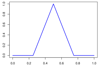
(a) When the template is Lipschitz, and the other model components satisfy some mild assumptions, the model is ‘smooth’. The M-estimator is $\sqrt{n}$-consistent and asymptotically normal.

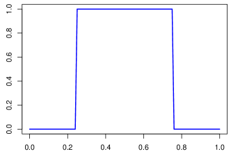
(b) When the template is piecewise Lipschitz with at least one discontinuity, and the other model components satisfy some mild assumptions, the M-estimator is $n$-consistent and its asymptotic distribution, although not well-defined, is essentially the minimum of a marked Poisson process.

Figure 1: Two emblematic templates: a Lipschitz template on the left representing a ‘smooth’ setting, and a piecewise Lipschitz template on the right representing a ‘non-smooth’ setting.

2 Consistency

Having chosen to work with a particular loss function ${\sf L}$, define

$$m_{\theta}(x,y):={\sf L}(y-f(x-\theta)),$$ (7)

so that the estimator in (2) can be equivalently defined via

$$\hat{\theta}_{n}:=\operatorname*{arg\,min}_{\theta}\widehat{M}_{n}(\theta), \widehat{M}_{n}(\theta):=\frac{1}{n}\sum_{i=1}^{n}m_{\theta}(X_{i},Y_{i}),$$ (8)

where we have added the subscript $n$ to emphasize that the estimator is being computed on a sample of size $n$. So that we can carry out a large-sample analysis, we require that

$$\operatorname{\mathbb{E}}[m_{\theta}(X,Y)]<\infty,\quad\text{for all $\theta$},$$ (9)

where $(X,Y)$ is a generic observation and $\operatorname{\mathbb{E}}$ is the expectation with respect to the distribution of $(X,Y)$ under $\theta^{*}$, the true value of the shift. Under Asumption 1 and Asumption 4, the following can be seen to be sufficient

$$\operatorname{\mathbb{E}}[{\sf L}(Z)]<\infty,$$ (10)

where $Z$ is a generic noise random variable. For the squared error loss, the requirement is that the noise distribution have a finite second moment, while for the absolute-value and the Huber losses, the requirement is that the noise distribution have a finite first moment, and the requirement is automatically fulfilled when the loss is bounded. When (9) holds, $\widehat{M}_{n}(\theta)$ has a well-defined expectation under $\theta^{*}$ given by

$$M(\theta):=\operatorname{\mathbb{E}}[m_{\theta}(X,Y)].$$ (11)

In particular, for any $\theta$, $\widehat{M}_{n}(\theta)$ converges to $M(\theta)$ in probability by the law of large numbers, and thus one anticipates that, under some additional conditions perhaps, $\hat{\theta}_{n}$ would converge to a minimizer of $M$.

Assumption 5.

$M$ introduced in (11) is well-defined. Moreover, $\theta^{*}$ is the unique minimum of $M$ and $\inf\{M(\theta):|\theta-\theta^{*}|\geq\delta\}>M(\theta^{*})$ for every $\delta>0$.

With Asumption 3 and Asumption 4 in place, Asumption 5 is satisfied for the squared error, absolute-value, and Huber losses, and also for the Tukey loss if in addition the noise distribution is unimodal. See Lemma A.1.

Theorem 2.1 (Consistency).

Under the basic assumptions, $\hat{\theta}_{n}$ is consistent for $\theta^{*}$.

Proof.

The requirements for applying (van der Vaart, 1998, Th 5.7) are (i) $M$ takes its minimum at $\theta^{*}$ and is bounded away from its minimum at $\theta$ away from $\theta^{*}$ — which is implied in Asumption 5; and (ii) $\widehat{M}_{n}$ converges to $M$ uniformly, meaning that

$$\sup_{\theta}|\widehat{M}_{n}(\theta)-M(\theta)|\to 0,\quad n\to\infty,$$ (12)

in probability — which is due to the fact that the function class $\{m_{\theta}:\theta\in\mathbb{R}\}$ is Glivenko–Cantelli. This latter property is essentially established in (van der Vaart, 1998, Ex 19.8), where the assumption of continuity can be relaxed to continuity almost everywhere, which holds here by the fact that $f$ and ${\sf L}$ are at least piecewise continuous. (van der Vaart, 1998, Ex 19.8) works under the assumption that the parameter space is compact, and this is effectively the case here. ∎

3 Smooth setting

We start by analyzing the situation where $f$ is Lipschitz. It turns out that, when this is the case, under mild assumptions on the design and noise distributions as well as the loss function, the situation is ‘standard’ for a parametric model in the sense that the M-estimator is $\sqrt{n}$ - consistent and asymptotically normal. In addition, the model is ‘smooth’ in the sense of being quadratic mean differentiable (van der Vaart, 1998, Sec 5.5), which then implies that the maximum likelihood estimator — which can coincide with the M-estimator as mentioned in Remark 1.1 — is locally asymptotic minimax and efficient.

Remark 3.1.

We remind the reader that a Lipschitz function is differentiable almost everywhere with a bounded derivative, and that it is the integral of that derivative (i.e., it is absolutely continuous). For such a function $g$, we will denote by $g^{\prime}$ its derivative and by $|g^{\prime}|_{\infty}$ its Lipschitz constant (which bounds the derivative when it exists).

3.1 Asymptotic normality

We first consider a smooth loss, encompassing the squared error loss and the Huber loss, among others.

Theorem 3.2.

Suppose the basic assumptions are in place. Assume, in addition, that $f$ is Lipschitz, that $\lambda$ is Lipschitz on an open set containing the support of $f(\cdot-\theta^{*})$, and that ${\sf L}$ has a Lipschitz first derivative. Unless ${\sf L}$ itself is Lipschitz, assume that the noise distribution has finite second moment. Then $\sqrt{n}(\hat{\theta}_{n}-\theta^{*})$ is asymptotically normal with mean $0$ and variance $\tau^{2}$, with

$$\tau^{2}:=\frac{C_{\phi,{\sf L}}}{\operatorname{\mathbb{E}}[f^{\prime}(X-\theta^{*})^{2}]},\quad C_{\phi,{\sf L}}:=\frac{\operatorname{\mathbb{E}}[{\sf L}^{\prime}(Z)^{2}]}{\operatorname{\mathbb{E}}[{\sf L}^{\prime\prime}(Z)]^{2}}.$$ (13)

Remark 3.3.

The assumption that $\lambda$ is Lipschitz is not needed, as can be seen by using the approach of Section 4. However, it makes for a particularly straightforward proof.

Proof.

Assume $\theta^{*}=0$ without loss of generality. In (van der Vaart, 1998, Th 5.23), the first condition is that $\theta\mapsto m_{\theta}(x,y)$ be differentiable at $0$ for almost every $(x,y)$, which is clearly the case here, as it is differentiable with derivative

$$\dot{m}_{\theta}(x,y)=f^{\prime}(x-\theta){\sf L}^{\prime}(y-f(x-\theta)),$$ (14)

If ${\sf L}$ itself is Lipschitz, we have

$$|m_{\theta_{1}}(x,y)-m_{\theta_{2}}(x,y)| =|{\sf L}(y-f(x-\theta_{1}))-{\sf L}(y-f(x-\theta_{2}))|$$ (15)

$$\leq|{\sf L}^{\prime}|_{\infty}\,|f(x-\theta_{1})-f(x-\theta_{2})|$$ (16)

$$\leq|{\sf L}^{\prime}|_{\infty}\,|f^{\prime}|_{\infty}|\theta_{1}-\theta_{2}|$$ (17)

$$=:\overline{m}(x,y)\,|\theta_{1}-\theta_{2}|.$$ (18)

Otherwise, we have

$$|m_{\theta_{1}}(x,y)-m_{\theta_{2}}(x,y)| =|{\sf L}(y-f(x-\theta_{1}))-{\sf L}(y-f(x-\theta_{2}))|$$ (19)

$$\leq|{\sf L}^{\prime\prime}|_{\infty}\,(|y-f(x)|+2|f|_{\infty})\,|f^{\prime}|_{\infty}\,|\theta_{1}-\theta_{2}|$$ (20)

$$=:\overline{m}(x,y)\,|\theta_{1}-\theta_{2}|.$$ (21)

In the second inequality we used the fact that $|y-f(x-\theta)|\leq|y-f(x)|+|f|_{\infty}$ for all $\theta$ and that $|{\sf L}^{\prime}(y)|\leq|{\sf L}^{\prime\prime}|_{\infty}|y|$ for all $y$ since ${\sf L}^{\prime}(0)=0$. In either case, $\operatorname{\mathbb{E}}[\overline{m}(X,Y)^{2}]<\infty$, so that the second condition of (van der Vaart, 1998, Th 5.23) is satisfied.

The third condition in that theorem is that $M(\theta)$ admits a Taylor expansion of order two at $\theta^{*}$ with nonzero second order term. Our assumptions imply that we can differentiate once inside the expectation defining $M$ to obtain its first derivative. To see this, note that $\theta\mapsto m_{\theta}(x,y)$ has first derivative given by (14), which is dominated by $|f^{\prime}|_{\infty}|{\sf L}^{\prime}|_{\infty}$ if ${\sf L}$ is Lipschitz, and by $|f^{\prime}|_{\infty}|{\sf L}^{\prime\prime}|_{\infty}(|y-f(x)|+2|f|_{\infty})$ otherwise, which is integrable in either case. Hence, $M$ is differentiable, with

$$M^{\prime}(\theta) =\operatorname{\mathbb{E}}[\dot{m}_{\theta}(X,Y)]$$

$$=\operatorname{\mathbb{E}}[f^{\prime}(X-\theta){\sf L}^{\prime}(Y-f(X-\theta))]$$

$$=\int\int f^{\prime}(x-\theta){\sf L}^{\prime}(f(x)-f(x-\theta)+z)\phi(z)\lambda(x){\rm d}z{\rm d}x$$

$$=\int\int f^{\prime}(x){\sf L}^{\prime}(f(x+\theta)-f(x)+z)\phi(z)\lambda(x+\theta){\rm d}z{\rm d}x.$$

Thus, by applying a simple change of variables we have transferred $\theta$ away from $f^{\prime}$ at the cost of burdening $\lambda$. But our assumptions are exactly what we need to differentiate inside the integral, since the integrand is differentiable with derivative

$$f^{\prime}(x)\big{\{}f^{\prime}(x+\theta){\sf L}^{\prime\prime}(f(x+\theta)-f(x)+z)\lambda(x+\theta)+{\sf L}^{\prime}(f(x+\theta)-f(x)+z)\lambda^{\prime}(x+\theta)\big{\}}\phi(z),$$ (22)

which is dominated by

$$|f^{\prime}|_{\infty}\big{\{}|f^{\prime}|_{\infty}|{\sf L}^{\prime\prime}|_{\infty}|\lambda|_{\infty}+|{\sf L}^{\prime}|_{\infty}|\lambda^{\prime}|_{\infty}\big{\}}\phi(z),$$ (23)

if ${\sf L}$ is Lipschitz, and otherwise by

$$|f^{\prime}|_{\infty}\big{\{}|f^{\prime}|_{\infty}|{\sf L}^{\prime\prime}|_{\infty}|\lambda|_{\infty}+|{\sf L}^{\prime\prime}|_{\infty}(|z|+2|f|_{\infty})|\lambda^{\prime}|_{\infty}\big{\}}\phi(z),$$ (24)

and this is integrable in either case. (Recall that $\lambda$ is compactly supported.) Hence, $M$ is indeed twice differentiable, with

$$M^{\prime\prime}(0) =\int\int f^{\prime}(x)\big{\{}f^{\prime}(x){\sf L}^{\prime\prime}(z)\lambda(x)+{\sf L}^{\prime}(z)\lambda^{\prime}(x)\big{\}}\phi(z){\rm d}z{\rm d}x$$

$$=\int\int f^{\prime}(x)^{2}{\sf L}^{\prime\prime}(z)\lambda(x)\phi(z){\rm d}z{\rm d}x$$

$$=\operatorname{\mathbb{E}}[f^{\prime}(X)^{2}]\operatorname{\mathbb{E}}[{\sf L}^{\prime\prime}(Z)],$$

because $\int_{-\infty}^{\infty}{\sf L}^{\prime}(z)\phi(z){\rm d}z=0$ due to the fact that ${\sf L}^{\prime}$ is odd and $\phi$ is even.

The last condition in (van der Vaart, 1998, Th 5.23) is that $\hat{\theta}_{n}$ be consistent, which we have already established in Theorem 2.1.

Therefore, (van der Vaart, 1998, Th 5.23) applies, and implies that $\sqrt{n}(\hat{\theta}_{n}-\theta^{*})$ is asymptotically normal with mean $0$ and variance

$$\frac{\operatorname{\mathbb{E}}[\dot{m}_{0}(X,Y)^{2}]}{M^{\prime\prime}(0)^{2}},$$ (25)

the latter reducing to (13) after some simplifications. ∎

Theorem 3.2 applies to the squared error, the Huber, and the Tukey losses with no additional conditions other than the basic assumptions. For squared error loss, the factor $C_{\phi,{\sf L}}$ in the asymptotic variance is given by

$$C_{\rm squared}:=\operatorname{\mathbb{E}}[Z^{2}]=\text{noise variance}.$$ (26)

For the Huber loss (5),

$$C_{\rm huber}:=\frac{\operatorname{\mathbb{E}}[Z^{2}\wedge c^{2}]}{\operatorname{\mathbb{P}}(|Z|\leq c)^{2}}.$$ (27)

Theorem 3.2 does not apply to the absolute-value loss. But very similar arguments can be used to obtain a normal limit distribution for that loss.

Theorem 3.4.

In the context of Theorem 3.2, assume that ${\sf L}$ is the absolute-value loss and that $\phi$ is continuous and strictly positive at the origin. Then the same conclusion holds with

$$C_{\phi,{\sf L}}=\frac{1}{4\phi(0)^{2}}.$$ (28)

Proof.

Assume $\theta^{*}=0$ without loss of generality.

In (van der Vaart, 1998, Th 5.23), the first condition is that $\theta\mapsto m_{\theta}(x,y)$ be differentiable at $0$ for almost every $(x,y)$, which is clearly the case here, as it is differentiable with derivative

$$\dot{m}_{\theta}(x,y)=f^{\prime}(x-\theta)\operatorname{sign}(y-f(x-\theta)),$$ (29)

We also have

$$|m_{\theta_{1}}(x,y)-m_{\theta_{2}}(x,y)| =\big{|}|y-f(x-\theta_{1})|-|y-f(x-\theta_{2})|\big{|}$$ (30)

$$\leq|f(x-\theta_{1})-f(x-\theta_{2})|$$ (31)

$$\leq|f^{\prime}|_{\infty}\,|\theta_{1}-\theta_{2}|.$$ (32)

Hence, the second condition of (van der Vaart, 1998, Th 5.23) is satisfied.

Our assumptions imply that we can differentiate once inside the expectation defining $M$ to obtain its first derivative

$$M^{\prime}(\theta) =\operatorname{\mathbb{E}}[\dot{m}_{\theta}(X,Y)]$$

$$=\operatorname{\mathbb{E}}[f^{\prime}(X-\theta)\operatorname{sign}(Y-f(X-\theta))]$$

$$=\int\int f^{\prime}(x-\theta)\operatorname{sign}(f(x)-f(x-\theta)+z)\phi(z)\lambda(x){\rm d}z{\rm d}x$$

$$=\int\int f^{\prime}(x)\operatorname{sign}(f(x+\theta)-f(x)+z)\phi(z)\lambda(x+\theta){\rm d}z{\rm d}x$$

$$=\int f^{\prime}(x)\big{(}1-2\Phi(f(x)-f(x+\theta))\big{)}\lambda(x+\theta){\rm d}x,$$

where $\Phi(z):=\int_{-\infty}^{z}\phi(u){\rm d}u$. The integrand is differentiable with derivative

$$f^{\prime}(x)\big{\{}2f^{\prime}(x+\theta)\phi(f(x)-f(x+\theta))\lambda(x+\theta)+\big{(}1-2\Phi(f(x)-f(x+\theta))\big{)}\lambda^{\prime}(x+\theta)\big{\}}$$ (33)

which is bounded and therefore dominated as $\theta$ varies. The remaining arguments are as in the proof of Theorem 3.2. ∎

Remark 3.5.

The expression for the asymptotic variance for the absolute-value loss given could have been anticipated based on the corresponding expression for the Huber loss given in (27). Indeed, as $c\to 0$, the Huber loss (5) converges pointwise to the absolute-value loss, so that we could have speculated that the same would be true for the asymptotic variances. It turns out that this prediction would have been correct, as it is indeed the case that

$$\operatorname{\mathbb{E}}[Z^{2}\wedge c^{2}]/\operatorname{\mathbb{P}}(|Z|\leq c)^{2}\xrightarrow{c\to 0}1/4\phi(0)^{2}$$ (34)

when $\phi$ may be taken continuous at the origin. It is also the case that the Huber loss converges pointwise to the squared error loss when $c\to\infty$ instead, and that

$$\operatorname{\mathbb{E}}[Z^{2}\wedge c^{2}]/\operatorname{\mathbb{P}}(|Z|\leq c)^{2}\xrightarrow{c\to\infty}\operatorname{\mathbb{E}}[Z^{2}].$$ (35)

Remark 3.6.

The constant $C_{\phi,{\sf L}}$ in Theorem 3.2 and Theorem 3.4 is the asymptotic variance in the classical location model where $Y_{i}=\theta^{*}+Z_{i}$. The only way in which the model we assume (1) is different asymptotically is in the denominator in (13).

3.2 Local asymptotic minimaxity

Under the same smoothness condition on the template as in Section 3.1, namely, assuming that $f$ has a bounded derivative, and under some smoothness assumption on the noise density (and not the design density this time), the statistical model is smooth in the sense of being quadratic mean differentiable (QMD). Indeed, under $\theta$, the joint distribution of $(X,Y)$ has density

$$p_{\theta}(x,y):=\lambda(x)\phi(y-f(x-\theta)).$$ (36)

The function $\theta\mapsto p_{\theta}(x,y)$ is differentiable when $f$ and $\phi$ are. The information at $\theta$ is defined as

$$I_{\theta} :=\int\int\frac{\dot{p}_{\theta}(x,y)^{2}}{p_{\theta}(x,y)}{\rm d}y{\rm d}x$$ (37)

$$=\int\int\frac{\lambda(x)f^{\prime}(x-\theta)^{2}\phi^{\prime}(y-f(x-\theta))^{2}}{\phi(y-f(x-\theta))}{\rm d}y{\rm d}x$$ (38)

$$=\int\lambda(x)f^{\prime}(x-\theta)^{2}{\rm d}x\times\int\frac{\phi^{\prime}(y)^{2}}{\phi(y)}{\rm d}y,$$ (39)

and when it is finite and continuous, as it is the case here, the model is QMD (Lehmann and Romano, 2005, Th 12.2.1).

When a model is QMD then, under additional mild assumptions, the MLE behaves in a standard way: If $\hat{\theta}_{n}$ denotes the MLE, then $\sqrt{n}(\hat{\theta}_{n}-\theta)$ is asymptotically normal with zero mean and variance $1/I_{\theta}$ under $\theta$. These additional assumptions are fulfilled, for example, when $(x,y)\mapsto\sup_{\theta}\,\dot{p}_{\theta}(x,y)^{2}/p_{\theta}(x,y)$ is square integrable (van der Vaart, 1998, Th 5.39). If the M-estimator is the MLE, meaning when $\phi(y)\propto\exp(-{\sf L}(y))$, this is the case under the conditions of Theorem 3.2.

It turns out this behavior is best possible asymptotically as we describe next. In the present context, we say that an estimator $\hat{\theta}_{n}$ is locally asymptotically minimax (LAM) at some $\theta_{0}$ if

$$\lim_{\delta\to 0}\liminf_{n\to\infty}\sup_{|\theta-\theta_{0}|<\delta}\operatorname{\mathbb{E}}_{\theta}\big{[}\sqrt{n}|\hat{\theta}_{n}-\theta|\big{]}$$ (40)

achieves the minimum possible value among all estimators. Here $\operatorname{\mathbb{E}}_{\theta}$ denotes the expectation with respect to $p_{\theta}$. We say that an estimator is LAM if it is LAM at every $\theta_{0}$. And, indeed, the MLE is LAM under the same conditions, meaning those of (van der Vaart, 1998, Th 5.39), which again hold in the context of Theorem 3.2. Hence, we may conclude the following.

Theorem 3.7.

Under the conditions of Theorem 3.2, and assuming in addition that $\phi(y)\propto\exp(-{\sf L}(y))$, the M-estimator is LAM.

3.3 Relative efficiency

Although the Huber estimator and the least absolute-value estimator can be motivated as maximum likelihood estimators in their own right, they are often considered as robust compromises to the otherwise preferred least squares estimator. The rationale behind this is in general flimsy, as it amounts to assuming that the noise distribution is Gaussian, as in that case the least squares estimator is the MLE and thus LAM. In signal processing applications, however, the normal assumption can be justified. In any case, this is the perspective we adopt.

We assume therefore that the noise distribution is Gaussian, making the least squares estimator the gold standard for asymptotic comparisons. In that context, if $\hat{\theta}_{n}$ is another estimator such that $\sqrt{n}(\hat{\theta}_{n}-\theta)$ is asymptotically normal with mean 0 and variance $\tau^{2}$ under $\theta$, then its relative efficiency with respect to the MLE is

$$\frac{\tau^{2}}{\tau^{2}_{\rm mle}},$$ (41)

and gives, asymptotically, how many more samples this estimator requires in order to achieve the same precision as the MLE in terms of the width of asymptotically-valid confidence intervals at an arbitrary level of confidence. In our context, $\tau_{\rm mle}$ is obtained from (13) with (26).

Using the expression (27), the relative efficiency of the Huber estimator with parameter $c$ is

$$\frac{\operatorname{\mathbb{E}}[Z^{2}\wedge c^{2}]}{\operatorname{\mathbb{E}}[Z^{2}]\operatorname{\mathbb{P}}(|Z|\leq c)^{2}}.$$ (42)

As anticipated, this is greater than 1 for all values of $c$ and converges to 1 as $c\to\infty$ (as the Huber loss converges to the squared error loss). Using the expression (28), the relative efficiency of the least absolute-value estimator is

$$\frac{1}{4\phi(0)^{2}\operatorname{\mathbb{E}}[Z^{2}]}.$$ (43)

In line with Remark 3.6, in both cases we recover the relative efficiency for the problem of estimating a normal mean.

3.4 Finite-sample minimaxity

When the model is smooth, the M-estimator is locally asymptotically minimax when it is the MLE, as we saw in Section 3.2, and more generally achieves the optimal $\sqrt{n}$ rate of convergence only losing in the leading constant, as detailed in Section 3.3. What about in finite samples?

In the present context, we define the risk of an estimator $\hat{\theta}_{n}$ at $\theta$ as

$${\sf risk}(\hat{\theta}_{n},\theta):=\operatorname{\mathbb{E}}_{\theta}\big{[}|\hat{\theta}_{n}-\theta|\big{]}.$$ (44)

The minimax risk is then defined as

$$R_{n}^{*}:=\inf_{\hat{\theta}_{n}}\sup_{\theta}{\sf risk}(\hat{\theta}_{n},\theta),$$ (45)

where the infimum is over all estimators taking in a sample of size $n$.

Lemma 3.8.

Suppose the basic assumptions are in place. Assume, in addition, that $f$ is Lipschitz, that $\lambda$ is Lipschitz on an open set containing the support of $f(\cdot-\theta^{*})$, and that $t\mapsto B(t):=\int\phi(y)\log\phi(y-t){\rm d}y$ has a derivative which is Lipschitz near the origin. Then the minimax risk satisfies $\sqrt{n}R_{n}^{*}\gtrsim 1$.

Proof.

Assume without loss of generality that $\theta^{*}=0$. Recall the notation used for the joint density of $(X,Y)$ set in (36). By (Tsybakov, 2009, Th 2.1 and Th 2.2), it suffices to prove that ${\sf KL}(p_{\theta},p_{0})\lesssim 1/n$ when $\sqrt{n}|\theta|\lesssim 1$. Here ${\sf KL}$ denotes the Kullback–Leibler divergence. We have

$${\sf KL}(p_{\theta},p_{0})=A(\theta)-A(0),$$ (46)

where

$$A(\theta) :=\operatorname{\mathbb{E}}[-\log p_{\theta}(X,Y)]$$ (47)

$$=-\int B(f(x-\theta)-f(x))\lambda(x){\rm d}x.$$ (48)

Note that $|f(x-\theta)-f(x)|\leq|f^{\prime}|_{\infty}|\theta|$ and that $\theta$ is taken small. Hence, since $B$ is continuously differentiably in a neighborhood of the origin and $f$ is almost surely differentiable, $\theta\mapsto B(f(x-\theta)-f(x))\lambda(x)$ is almost surely differentiable near the origin. Its derivative is

$$f^{\prime}(x-\theta)B^{\prime}(f(x-\theta)-f(x))\lambda(x),$$ (49)

which is bounded since $f^{\prime}$ and $\lambda$ are. Also, $B^{\prime}$ is continuous and therefore locally bounded. Hence, by dominated convergence, $A$ is differentiable with

$$A^{\prime}(\theta) =\int f^{\prime}(x-\theta)B^{\prime}(f(x-\theta)-f(x))\lambda(x){\rm d}x$$ (50)

$$=\int f^{\prime}(x)B^{\prime}(f(x)-f(x+\theta))\lambda(x+\theta){\rm d}x,$$ (51)

after a change of variable. We also have that $\theta\mapsto f^{\prime}(x)B^{\prime}(f(x)-f(x+\theta))\lambda(x+\theta)$ is almost surely differentiable near the origin, with derivative

$$f^{\prime}(x)\big{\{}-f^{\prime}(x+\theta)B^{\prime\prime}(f(x)-f(x+\theta))\lambda(x+\theta)+B^{\prime}(f(x)-f(x+\theta))\lambda^{\prime}(x+\theta)\big{\}},$$ (52)

which is bounded for similar reasons. Hence, by dominated convergence, $A$ is twice differentiable with bounded second derivative. Note that $A^{\prime}(0)=B^{\prime}(0)\int f^{\prime}(x)\lambda(x){\rm d}x$ with $B^{\prime}(0)=0$ since $B$ is differentiable and attains its maximum at $0$, the latter because $B(0)-B(t)=\int\phi(y)\log(\phi(y)/\phi(y-t)){\rm d}y$ is the Kullback–Leibler divergence from $\phi(\cdot-t)$ to $\phi$. We thus obtain

$$A(\theta)-A(0)\leq\tfrac{1}{2}|A^{\prime\prime}|_{\infty}\theta^{2}.$$ (53)

This in turn implies that ${\sf KL}(p_{\theta},p_{0})\leq C\theta^{2}$ for some $C>0$. And $C\theta^{2}\leq 1/n$ when $\sqrt{n}|\theta|\leq 1/\sqrt{C}$. ∎

Hence, when the model is smooth, the minimax rate of convergence is also $\sqrt{n}$. And this rate is achieved by the M-estimator under essentially the same conditions.

Corollary 3.9 (Minimaxity).

Assume that the conditions of Theorem 3.2 or Theorem 3.4 hold, as well as those of Lemma 3.8. Then the M-estimator achieves the minimax convergence rate.

Proof.

It turns out that under the conditions of Theorem 3.2 or Theorem 3.4, the M-estimator satisfies (van der Vaart, 1998, Cor 5.53)

$$\operatorname{\mathbb{E}}_{\theta}[\sqrt{n}|\hat{\theta}_{n}-\theta|]=O(1).$$ (54)

(Note that this is not a consequence of the normal limit established in Theorem 3.2 or Theorem 3.4.) In our case, we can bound the expectation in (54) uniformly over $\theta$. This follows trivially from the arguments provided in the proof of (van der Vaart, 1998, Cor 5.53) and further details are omitted. Hence, $\sup_{\theta}{\sf risk}(\hat{\theta}_{n},\theta)=O(1/\sqrt{n})$, and in particular, $\hat{\theta}_{n}$ achieves the minimax convergence rate established in Lemma 3.8. ∎

4 Non-smooth setting

When $f$ is not Lipschitz, the situation can be nonstandard. We saw in Theorem 2.1 that the M-estimator remains consistent under the basic assumptions, but it turns out that it can have a consistency rate other than $\sqrt{n}$. Because nonstandard, the analysis is a little bit more involved, yet as it turns out all the tools we need are again available in (van der Vaart, 1998). The model is no longer smooth and we do not go into questions of local asymptotic minimaxity or relative efficiency. However, it turns out that the M-estimator remains rate-minimax.

Although other situations may be of interest, for the sake of concreteness we will consider two cases (and some sub-cases). In the first case, we take $f$ to be $\alpha$-Holder for some $0<\alpha\leq 1$, meaning

$$H:=\sup_{x_{1},x_{2}}\frac{|f(x_{1})-f(x_{2})|}{|x_{1}-x_{2}|^{\alpha}}<\infty.$$ (55)

When this holds for $\alpha=1$ the function is simply Lipschitz. In the second case, we take $f$ to be piecewise $\alpha$-Holder. We will let $\mathcal{D}$ denote the discontinuity set of $f$ which, remember, we are assuming is finite.

Everywhere, the basic assumptions are in place.

4.1 Preliminaries

We start with some preliminary results from which everything else follows. The following function will play an important role

$$\Delta(\theta_{1},\theta_{2})=\int(f(x-\theta_{1})-f(x-\theta_{2}))^{2}\lambda(x){\rm d}x.$$ (56)

We will also use the following notation

$$\tilde{m}_{\theta}(x,z)={\sf L}(z+f(x-\theta^{*})-f(x-\theta)),$$ (57)

which is useful because $m_{\theta}(x,y)=\tilde{m}_{\theta}(x,y-f(x-\theta^{*}))$.

The first result is an expansion of the function $M$ of (11).

Lemma 4.1.

If ${\sf L}$ has a bounded and almost everywhere continuous second derivative, then

$$M(\theta)=M(\theta^{*})+A(\theta)\Delta(\theta,\theta^{*}),$$ (58)

where $A$ is bounded and satisfies $A(\theta)\to C_{0}:=\tfrac{1}{2}\int L^{\prime\prime}\phi$ as $\theta\to\theta^{*}$. If ${\sf L}$ is the absolute-value loss, and $\phi$ is locally bounded and continuous at 0, then this continues to holds, except that $C_{0}:=\phi(0)$.

Proof.

Assume $\theta^{*}=0$ without loss of generality and let $\Delta(\theta)$ be short for $\Delta(\theta,\theta^{*})$. We start with the first situation. Motivated by the fact that $f(x)-f(x-\theta)$ tends to be small when $\theta$ is small, we derive

$$\tilde{m}_{\theta}(x,z) ={\sf L}(z+f(x)-f(x-\theta))$$ (59)

$$={\sf L}(z)+{\sf L}^{\prime}(z)(f(x)-f(x-\theta))+\tfrac{1}{2}{\sf L}^{\prime\prime}(z+\zeta(z,x,\theta))(f(x)-f(x-\theta))^{2},$$ (60)

for some $|\zeta(z,x,\theta)|\leq|f(x)-f(x-\theta)|$. Integrating over $x$ and $z$, we obtain

$$M(\theta) =M(0)+\int\int_{\mathbb{R}}\tfrac{1}{2}{\sf L}^{\prime\prime}(z+\zeta(z,x,\theta))(f(x)-f(x-\theta))^{2}\phi(z)\lambda(x){\rm d}z{\rm d}x$$

$$=M(0)+C_{0}\Delta(\theta)\pm\int\int_{\mathbb{R}}\gamma(z,|f(x)-f(x-\theta)|)(f(x)-f(x-\theta))^{2}\phi(z)\lambda(x){\rm d}z{\rm d}x,$$

where we have used the fact that $\int_{\mathbb{R}}{\sf L}^{\prime}(z)\phi(z){\rm d}z=0$, and where we used the notation

$$\gamma(z,a):=\sup_{|b|\leq a}|{\sf L}^{\prime\prime}(z+b)-{\sf L}^{\prime\prime}(z)|.$$ (61)

By our assumptions on ${\sf L}^{\prime\prime}$, $\gamma(z,a)\to 0$ when $a\to 0$ for almost every $z$. In addition, $\gamma$ is uniformly bounded. Hence, by dominated convergence, the last integral is $o(\Delta(\theta))$ as $\theta\to 0$.

We now turn to the situation where ${\sf L}$ is the absolute-value loss. We first note that

$$\int_{\mathbb{R}}|z+a|\phi(z){\rm d}z=2\Phi_{2}(z)+a,$$ (62)

where

$$\Phi_{2}(z):=\int_{-\infty}^{z}\Phi(u){\rm d}u,\quad\Phi(z):=\int_{-\infty}^{z}\phi(u){\rm d}u.$$ (63)

Note that $\Phi_{2}^{\prime}=\Phi$ and $\Phi_{2}^{\prime\prime}=\phi$. Using this, we derive

$$M(\theta) =M(0)+\int\big{\{}2\big{[}\Phi_{2}(f(x)-f(x-\theta))-\Phi_{2}(0)\big{]}+f(x)-f(x-\theta)\big{\}}{\rm d}x$$

$$=M(0)+C_{0}\Delta(\theta)+\int\phi(\zeta(x,\theta))(f(x)-f(x-\theta))^{2}\lambda(x){\rm d}x,$$

for some $|\zeta(x,\theta)|\leq|f(x)-f(x-\theta)|$. Note that $|\zeta(x,\theta)|\leq 2|f|_{\infty}$, so that $\phi(\zeta(x,\theta))$ is bounded. Moreover, by the fact that $\phi$ is continuous at 0, and that $f$ is continuous almost everywhere, it holds that $\phi(\zeta(x,\theta))\to 0$ as $\theta\to 0$ for almost all $x$. We can thus apply dominated convergence to find that the last integral is $o(\Delta(\theta))$ as $\theta\to 0$. ∎

Another notion that will be important is that of an envelope. We say that a function $V$ is an envelope for a function class $\mathcal{M}$ if any function in $\mathcal{M}$ is, in absolute value, pointwise bounded by $V$, or in formula, $|g(x)|\leq V(x)$ for all $x$ and all $g\in\mathcal{M}$. Below,

$$\mathcal{M}_{\delta}:=\big{\{}m_{\theta}-m_{\theta^{*}}:|\theta-\theta^{*}|\leq\delta\big{\}},$$ (64)

and

$$\mathcal{D}(\delta):=\{x=d+t:d\in\mathcal{D},|t|\leq\delta\},$$ (65)

where $\delta$ is thought of as being small.

Lemma 4.2.

Assume either that ${\sf L}$ has a Lipschitz derivative and that the noise distribution has finite second moment; or that ${\sf L}$ itself is Lipschitz. If $f$ is $\alpha$-Holder, then $\mathcal{M}_{\delta}$ admits an envelope of the form $V(x,y):=\overline{m}(z)\delta^{\alpha}$ where $z:=y-f(x-\theta^{*})$ and $\int\overline{m}^{2}\phi<\infty$. If $f$ is only piecewise $\alpha$-Holder, then the same is true but with $V(x,y):=\overline{m}(z)(\delta^{\alpha}+\mathbb{I}{\{x\in\mathcal{D}(\delta)\}})$.

Proof.

Assume $\theta^{*}=0$ without loss of generality, so that $\theta$ below satisfies $|\theta|\leq\delta$. For $x,y$, we let $z=y-f(x)$.

First, assume that $f$ is $\alpha$-Holder and let $H$ be defined as in (55). If the loss has a Lipschitz derivative, we have

$$|m_{\theta}(x,y)-m_{0}(x,y)| =|{\sf L}(z+f(x)-f(x-\theta))-{\sf L}(z)|$$

$$\leq|{\sf L}^{\prime}(z+\zeta)|\times|f(x)-f(x-\theta)|$$

$$\leq|{\sf L}^{\prime\prime}|_{\infty}(|z|+2|f|_{\infty})\times H|\theta|^{\alpha},$$

for some $|\zeta|\leq|f(x)-f(x-\theta)|\leq 2|f|_{\infty}$. We then conclude with $|\theta|\leq\delta$. If the loss is Lipshitz, we have

$$|m_{\theta}(x,y)-m_{0}(x,y)| \leq|L^{\prime}|_{\infty}|f(x)-f(x-\theta)|$$

$$\leq|L^{\prime}|_{\infty}H|\theta|^{\alpha},$$

and we conclude in the same way.

Next, assume that $f$ is piecewise $\alpha$-Holder. In this situation, let $H$ be defined as in (55), except away from discontinuities. Based on what we just did, it suffices to show that

$$|f(x)-f(x-\theta)|\leq C_{1}(\delta^{\alpha}+\mathbb{I}{\{x\in\mathcal{D}(\delta)\}}),$$ (66)

when $|\theta|\leq\delta$ for some constant $C_{1}$. Indeed, either there are no discontinuity point between $x$ and $x-\theta$, in which case $|f(x)-f(x-\theta)|\leq H|\theta|^{\alpha}$; or there is a discontinuity point, say $d$, between $x$ and $x-\theta$, so that $|x-d|\leq|\theta|\leq\delta$, implying that $|f(x)-f(x-\theta)|\leq 2|f|_{\infty}\mathbb{I}{\{x\in\mathcal{D}(\delta)\}}$. ∎

The next result is a complexity bound for $\mathcal{M}_{\delta}$. The complexity is in terms of bracketing numbers (van der Vaart, 1998, Sec 19.2). Two functions $g_{1},g_{2}$ such that $g_{1}\leq g_{2}$ pointwise define a bracket made of all functions $g$ such that $g_{1}\leq g\leq g_{2}$. It is said to be an $\varepsilon$-bracket with respect to $L^{2}(\mu)$, for a positive measure $\mu$, if $\int(g_{2}-g_{1})^{2}{\rm d}\mu\leq\varepsilon^{2}$. Given a class of functions $\mathcal{M}$, its $\varepsilon$-bracketing number with respect to $L^{2}(\mu)$ is the minimum number of $\varepsilon$-brackets needed to cover $\mathcal{M}$ (meaning to include any function in that class). In our context, the measure is the underlying sample distribution, meaning $p_{\theta*}$ in the notation introduced in (36). We let $N_{\delta}(\varepsilon)$ denote the $\varepsilon$-bracketing number of $\mathcal{M}_{\delta}$ with respect to $L^{2}(p_{\theta*})$.

Lemma 4.3.

There is a constant $C>0$ such that the following holds. Assume the loss is as in Lemma 4.2. If $f$ is $\alpha$-Holder, then $N_{\delta}(\varepsilon)\leq C\delta\varepsilon^{-1/\alpha}$. If $f$ is piecewise $\alpha$-Holder, and $\lambda$ is bounded, then $N_{\delta}(\varepsilon)\leq C\delta\varepsilon^{-1/(\alpha\wedge 1/2)}$.

Proof.

Assume $\theta^{*}=0$ without loss of generality, so that any value of the parameter below is in $[-\delta,\delta]$. Let $\theta_{j}=j\delta/k$ for $j=-k,\dots,k$. For $x,y$, we let $z=y-f(x)$ below. We rely on the proof of Lemma 4.2.

First, assume that $f$ is $\alpha$-Holder. We have

$$|m_{\theta}(x,y)-m_{\theta_{0}}(x,y)| \leq\overline{m}(z)|\theta-\theta_{0}|^{\alpha},$$

where $\overline{m}(z)$ is square integrable. For a given $\theta$, let $j$ be such that $|\theta-\theta_{j}|\leq\delta/k$. Then

$$|m_{\theta}(x,y)-m_{\theta_{j}}(x,y)| \leq\overline{m}(z)|\theta-\theta_{j}|^{\alpha}\leq\overline{m}(z)(\delta/k)^{\alpha},$$

implying that

$$A_{j}(x,y)\leq m_{\theta}(x,y)\leq B_{j}(x,y),$$ (67)

where

$$A_{j}(x,y) :=m_{\theta_{j}}(x,y)-\overline{m}(z)(\delta/k)^{\alpha}$$

$$B_{j}(x,y) :=m_{\theta_{j}}(x,y)+\overline{m}(z)(\delta/k)^{\alpha}.$$

Note that $B_{j}-A_{j}$ has $L^{2}$ norm of order $(\delta/k)^{\alpha}$ since $\overline{m}$ is square integrable. Choosing $k\geq C_{2}\delta/\varepsilon^{1/\alpha}$ for a large enough $C_{2}$ makes it an $\varepsilon$-bracket. And these $k$ brackets together cover $\mathcal{M}_{\delta}$.

Next, assume that $f$ is piecewise $\alpha$-Holder. Assume for expediency that $f$ has a single discontinuity, and let $d$ denote the location of that discontinuity. Following the corresponding arguments in Lemma 4.2, we can prove that

$$|m_{\theta}(x,y)-m_{\theta_{0}}(x,y)| \leq\overline{m}(z)(|\theta-\theta_{0}|^{\alpha}+\mathbb{I}{\{\theta_{0}\leq x-d\leq\theta\}}),$$

where $\overline{m}(z)$ is square integrable. For a given $\theta$, let $j$ be such that $\theta_{j}\leq\theta\leq\theta_{j+1}$. Then

$$A_{j}(x,y)\leq m_{\theta}(x,y)\leq B_{j}(x,y),$$ (68)

where

$$A_{j}(x,y) :=m_{\theta_{j}}(x,y)-\overline{m}(z)((\delta/k)^{\alpha}+\mathbb{I}{\{\theta_{j}\leq x-d\leq\theta_{j+1}\}})$$

$$B_{j}(x,y) :=m_{\theta_{j}}(x,y)+\overline{m}(z)((\delta/k)^{\alpha}+\mathbb{I}{\{\theta_{j}\leq x-d\leq\theta_{j+1}\}}).$$

The difference satisfies

$$\int(B_{j}(x,y)-A_{j}(x,y))^{2}\phi(y-f(x))\lambda(x){\rm d}y{\rm d}x$$

$$\leq 4\int\overline{m}(z)^{2}\phi(z){\rm d}z\times 2\int((\delta/k)^{2\alpha}+\mathbb{I}{\{\theta_{j}\leq x-d\leq\theta_{j+1}\}})\lambda(x){\rm d}x$$

$$\lesssim(\delta/k)^{2\alpha}+|\lambda|_{\infty}(\delta/k),$$

and so has $L^{2}$ norm of order $(\delta/k)^{\alpha}+(\delta/k)^{1/2}\asymp(\delta/k)^{\alpha\wedge 1/2}$, uniformly in $j$. Therefore, choosing $k\geq C_{3}\delta/\varepsilon^{1/(\alpha\wedge 1/2)}$ for a large enough $C_{3}$ ensures that $B_{j}-A_{j}$ has $L^{2}$ norm bounded by $\varepsilon$. And the $k$ brackets that these pairs of functions define as $j$ ranges through $\{-k,\dots,k\}$, together, cover the space $\mathcal{M}_{\delta}$. ∎

From here proceed in reverse order compared to Section 3: We first study the rate of convergence and then discuss the limit distribution.

4.2 Rate of convergence

The bracketing integral of a function class $\mathcal{M}$ with respect to $L^{2}(\mu)$ is defined as the integral of the square root of the logarithm of the corresponding $\varepsilon$-bracketing number as a function of $\varepsilon$. In particular, we introduce the bracketing integral of $\mathcal{M}_{\delta}$, denoted

$$J_{\delta}(t):=\int_{0}^{t}\sqrt{\log N_{\delta}(\varepsilon)}{\rm d}\varepsilon.$$ (69)

A simple adaptation of the arguments underlying (van der Vaart, 1998, Th 5.52), in combination with (van der Vaart, 1998, Cor 19.35), gives the following result.

Lemma 4.4.

Suppose there are constants $a>b\geq 0$ and $C>0$ such that, for $\delta>0$ small enough,

$$\inf_{|\theta-\theta^{*}|\geq\delta}M(\theta)-M(\theta^{*})\geq\delta^{a}/C,$$ (70)

and

$$J_{\delta}(\infty)\leq C\delta^{b}.$$ (71)

Then the M-estimator satisfies

$$\operatorname{\mathbb{E}}\big{[}n^{\frac{1}{2(a-b)}}|\hat{\theta}_{n}-\theta^{*}|\big{]}=O(1).$$ (72)

With the preceding lemmas, we are able to establish an upper bound on the rate of convergence of the M-estimator.

Theorem 4.5.

Suppose that either ${\sf L}$ has a bounded and almost everywhere continuous second derivative; or is the absolute-value loss and $\phi$ is locally bounded and continuous at 0.

• Suppose $f$ is $\alpha$-Holder and

  $$\sup_{|\theta-\theta^{*}|\leq\delta}\Delta(\theta,\theta^{*})\asymp\delta^{2\alpha}.$$ (73)

  Then the M-estimator is $r_{n}$-consistent with $r_{n}=n^{1/2\alpha}$.

• Suppose $f$ is discontinuous and piecewise $\alpha$-Holder with $\alpha\geq 1/2$, and $\lambda$ is bounded and continuous at the points of discontinuity of $f(\cdot-\theta^{*})$, and strictly positive at one or more of these locations. Then the M-estimator is $r_{n}$-consistent with $r_{n}=n$.

Proof.

Consider the first situation. We apply Lemma 4.4. By Lemma 4.1 and (73), the condition (70) is satisfied with $a=2\alpha$. Hence, it suffices to show that (71) holds with $b=\alpha$. Indeed, by Lemma 4.2, we have $J_{\delta}(\infty)=J_{\delta}(C\delta^{\alpha})$ for $C$ large enough, and by Lemma 4.3, we have

$$J_{\delta}(C\delta^{\alpha})\leq\int_{0}^{C\delta^{\alpha}}\sqrt{\log(C\delta/\varepsilon^{1/\alpha})}{\rm d}\varepsilon\asymp\delta^{\alpha}.$$ (74)

We now turn to the second situation. By of Lemma 4.2, we have $J_{\delta}(\infty)=J_{\delta}(C\delta^{1/2})$ for $C$ large enough, and by Lemma 4.3, we have

$$J_{\delta}(C\delta^{1/2})\leq\int_{0}^{C\delta^{1/2}}\sqrt{\log(C\delta/\varepsilon^{2})}{\rm d}\varepsilon\asymp\delta^{1/2},$$ (75)

so that (71) holds with $b=1/2$. It thus suffices to show that (70) holds with $a=1$. Assume for simplicity that $f$ has only one discontinuity, and therefore of the form $f(x)=f_{1}(x)\mathbb{I}{\{x<d\}}+f_{2}(x)\mathbb{I}{\{x\geq d\}}$ with $f_{1}$ and $f_{2}$ being $\alpha$-Holder. For example, consider a situation where $\theta>0=\theta^{*}$. We have

$$\Delta(\theta,\theta^{*})=\int_{-\infty}^{d}+\int_{d}^{d+\theta}+\int_{d+\theta}^{\infty}\quad(f(x)-f(x-\theta))^{2}\lambda(x){\rm d}x.$$ (76)

(In what follows, remember that $\lambda$ is compactly supported.) In the 1st and 3rd integral, $|f(x)-f(x-\theta)|\leq H|\theta|^{\alpha}$ since $f$ does not have a discontinuity over the corresponding ranges, $x\in[0,d)$ and $x\in(d+\theta,1]$, respectively. Hence, these two integrals are of order $|\theta|^{2\alpha}$, which is at most of order $O(\theta)$ since $\alpha\geq 1/2$. For the 2nd or middle integral, we use the fact that $(f(x)-f(x-\theta))\lambda(x)=(f_{2}(x)-f_{1}(x-\theta))^{2}\lambda(x)\to(f_{2}(d)-f_{1}(d))^{2}\lambda(d)$ when $x\in[d,d+\theta]$ and $\theta\to 0$, so that the integral is $\sim|\theta|(f_{2}(d)-f_{1}(d))^{2}\lambda(d)$ by dominated convergence. More generally, if $\mathcal{D}$ denotes the points of discontinuity of $f$, extending these arguments gives

$$\Delta(\theta,\theta^{*})\sim|\theta|D,\quad\text{as }\theta\to 0=\theta^{*},\quad\text{where }D:=\sum_{d\in\mathcal{D}}(f(d^{+})-f(d^{-}))^{2}\lambda(d)\ .$$ (77)

From this we conclude. ∎

Of course, we have only obtained an upper bound on the consistency rate. But as we will see in the next subsection, that rate is sharp.

Remark 4.6.

We note that (73) is not automatically satisfied even when the function $f$ is exactly $\alpha$-Holder (and not $(\alpha+\eta)$-Holder for any $\eta>0$). Indeed, consider the case where $f$ coincides near the origin with $x\mapsto|x|^{\alpha}$ for some fixed $0<\alpha<1$, and is otherwise Lipschitz. Then such an $f$ is exactly $\alpha$-Holder, and yet, it can be shown that

$$\sup_{|\theta-\theta^{*}|\leq\delta}\Delta(\theta,\theta^{*})\asymp\begin{cases}\delta^{2}&\text{if }\alpha>1/2,\\ \delta^{2}\log(1/\delta)&\text{if }\alpha=1/2,\\ \delta^{2\alpha+1}&\text{if }\alpha<1/2.\end{cases}$$ (78)

4.3 Minimaxity

We can easily adapt the arguments underlying the information bound stated in Lemma 3.8 to the settings that interest us in the present section where $f$ is not Lipschitz. We do so and obtain the following.

Lemma 4.7.

Suppose the basic assumptions are in place. Assume, in addition, that $\phi$ has finite first moment and that $B$ is as in Lemma 3.8. If $r_{n}$ is such that $\sup\{\Delta(\theta,\theta^{*}):r_{n}|\theta-\theta^{*}|\leq 1\}\lesssim 1/n$, the minimax rate satisfies $r_{n}R_{n}^{*}\gtrsim 1$.

Proof.

Assume without loss of generality that $\theta^{*}=0$ and let $\Delta(\theta)$ be short for $\Delta(\theta,\theta^{*})$. In the notation introduced in the proof of Lemma 3.8, it suffices to prove that $A(\theta)-A(0)\lesssim 1/n$ when $r_{n}|\theta|\leq 1$. We saw in the proof of that lemma that $B^{\prime}(0)=0$. This together with the fact that $B^{\prime}$ is Lipschitz near the origin implies that there is a positive constant $C_{1}$ such that $|B(t)-B(0)|\leq C_{1}t^{2}$ when $|t|$ is small enough. We use that to derive

$$A(\theta)-A(0) =\int\big{\{}B(0)-B(f(x-\theta)-f(x))\big{\}}\lambda(x){\rm d}x$$ (79)

$$\leq C_{1}\int(f(x-\theta)-f(x))^{2}\lambda(x){\rm d}x$$ (80)

$$=C_{1}\Delta(\theta).$$ (81)

From this we conclude. ∎

Corollary 4.8.

In the context of Lemma 4.7, if $f$ is $\alpha$-Holder, then $n^{1/2\alpha}R_{n}^{*}\gtrsim 1$; if instead $f$ is discontinuous and piecewise $\alpha$-Holder with $\alpha\geq 1/2$, then $nR_{n}^{*}\gtrsim 1$.

Proof.

As we saw in the proof of Theorem 4.5, if $f$ is $\alpha$-Holder, $\Delta(\theta,\theta^{*})\lesssim|\theta-\theta^{*}|^{2\alpha}$; while if instead $f$ is discontinuous and piecewise $\alpha$-Holder with $\alpha\geq 1/2$, $\Delta(\theta,\theta^{*})\lesssim|\theta-\theta^{*}|$. We then apply Lemma 4.7 to conclude. ∎

4.4 Limit distribution

To establish a limit distribution, we follow the standard strategy which starts by showing that a properly normalized version of the empirical process $\widehat{M}_{n}$ converges to a Gaussian process, and is followed by an application of the argmax continuous mapping theorem.

The following is a direct consequence of (van der Vaart, 1998, Th 19.28).

Lemma 4.9.

Consider a set of functions on some Euclidean space and let $\mu$ denote a Borel probability measure. Consider a class of functions $\mathcal{W}_{n,T}:=\{w_{n,t}:n\geq 1,t\in[-T,T]\}$ satisfying the following:

1. The class has a square integrable envelope.

2. The limit $g(t):=\lim_{n}\sqrt{n}\int w_{n,t}{\rm d}\mu$ is well-defined for all $t$.

3. There is a function $\omega_{1}$ with $\lim_{t\to 0+}\omega_{1}(t)=0$ and a sequence $\eta_{n}\to 0$ such that

   $$v_{n}(s,t):=\int(w_{n,s}-w_{n,t})^{2}{\rm d}\mu\leq\omega_{1}(|s-t|)+\eta_{n};$$ (82)

4. The limit $v(s,t):=\lim_{n}v_{n}(s,t)$ is well-defined for all $s,t$.

5. The class has bracketing integral $J_{n,T}(\delta)\leq\omega_{2}(\delta)$ for some function $\omega_{2}$ with $\lim_{t\to 0+}\omega_{2}(t)=0$.

Then $W_{n,t}:=\sum_{i=1}^{n}w_{n,t}$ converges weakly to $g(t)+G_{t}$ on $[-T,T]$, where $G_{t}$ denotes the centered Gaussian process with variance function $v$. Note that $v(s,t)\leq\omega_{1}(|s-t|)$.

The following is a special case of (van der Vaart, 1998, Cor 5.58).

Lemma 4.10.

Suppose that a sequence of processes $W_{n}$ defined on the real line converges weakly in the uniform topology on every bounded interval to a process $W$ with continuous sample paths each having a unique minimum point $h$ (almost surely). If $h_{n}$ minimizes $W_{n}$, and $(h_{n})$ is uniformly tight, then $h_{n}$ converges weakly to $h$.

We apply these two lemmas to obtain a limit distribution for the M-estimator when the template is $\alpha$-Holder. For expediency, we only consider smoother losses.

Theorem 4.11.

Suppose that ${\sf L}$ has a bounded and almost everywhere continuous second derivative. Assume that $f$ is $\alpha$-Holder and such that

$$r^{2\alpha}\Delta(\theta^{*}+s/r,\theta^{*}+t/r)\to\Delta_{0}(s,t),\quad r\to\infty,$$ (83)

where $\Delta_{0}$ is a continuous function such that $\Delta_{0}(s,t)\neq 0$ when $s\neq t$. Then $n^{1/2\alpha}(\hat{\theta}_{n}-\theta^{*})$ converges weakly to $\operatorname*{arg\,min}_{t}\{g(t)+G_{t}\}$ where $g(t):=C_{0}\Delta_{0}(t,0)$ with $C_{0}:=\tfrac{1}{2}\int L^{\prime\prime}\phi$ and $G_{t}$ is the centered Gaussian process on the real line with variance function $C_{1}\Delta_{0}(s,t)$ with $C_{1}:=\int({\sf L}^{\prime})^{2}\phi$.

Proof.

As usual, assume that $\theta^{*}=0$ without loss of generality, and let $z=y-f(x)$.

We first prove that the process $\sqrt{n}(\widehat{M}_{n}(t/r_{n})-\widehat{M}_{n}(0))$ — where $r_{n}=n^{1/2\alpha}$ is the rate of convergence established in Theorem 4.5 — converges weakly to $g(t)+G_{t}$. For this it is enough to prove that it converges on every interval of the form $[-T,T]$, and we do so by applying Lemma 4.9 with $w_{n,t}:=\sqrt{n}(m_{t/r_{n}}-m_{0})$. Note that $\mu=p_{0}$, the distribution of $(X,Y)$ under $\theta=0$. Lemma 4.2 and a rescaling argument gives (i). But to be sure, using Lemma 4.1, we have

$$|w_{n,t}(x,y)| \leq\sqrt{n}\big{\{}|{\sf L}^{\prime}(z)||f(x)-f(x-t/r_{n})|+\tfrac{1}{2}|{\sf L}^{\prime\prime}|_{\infty}(f(x)-f(x-t/r_{n}))^{2}\big{\}}$$ (84)

$$\leq\sqrt{n}\big{\{}|{\sf L}^{\prime}(z)|H(T/r_{n})^{\alpha}+\tfrac{1}{2}|{\sf L}^{\prime\prime}|_{\infty}(H(T/r_{n})^{\alpha})^{2}\big{\}}$$ (85)

$$\leq C({\sf L}^{\prime}(|z|)+1)=:\overline{w}(x,y).$$ (86)

We then conclude with the fact that $\overline{w}$ is square integrable by the usual assumptions.

For (ii), using Lemma 4.1, we have

$$\sqrt{n}\int w_{n,t}{\rm d}\mu =\sqrt{n}\times\sqrt{n}(M(t/r_{n})-M(0))$$ (87)

$$\sim nC_{0}\Delta(t/r_{n},0),\quad n\to\infty,$$ (88)

$$=nC_{0}r_{n}^{-2\alpha}r_{n}^{2\alpha}\Delta(t/r_{n},0)$$ (89)

$$\to C_{0}\Delta_{0}(t,0)=g(t),\quad n\to\infty.$$ (90)

For (iii), using (59), we have for $s,t\in[-T,T]$,

$$\int(w_{n,s}-w_{n,t})^{2}{\rm d}\mu =n\int(m_{s/r_{n}}-m_{t/r_{n}})^{2}{\rm d}p_{0}$$ (91)

$$\leq n\Big{[}2C_{1}\Delta(s/r_{n},t/r_{n})+|{\sf L}^{\prime\prime}|_{\infty}^{2}\{\Delta(s/r_{n},0)^{2}+\Delta(t/r_{n},0)^{2}\}\Big{]}$$ (92)

$$\leq n\Big{[}2C_{1}(H|s/r_{n}-t/r_{n}|^{\alpha})^{2}+|{\sf L}^{\prime\prime}|_{\infty}^{2}\{(H|s/r_{n}|^{\alpha})^{4}+(H|t/r_{n}|^{\alpha})^{4}\}\Big{]}$$ (93)

$$\leq nC\big{(}|s-t|^{2\alpha}/r_{n}^{2\alpha}+(T/r_{n})^{4\alpha}\big{)}$$ (94)

$$=C\big{(}|s-t|^{2\alpha}+T^{4\alpha}/n\big{)},$$ (95)

using the fact that $r_{n}^{2\alpha}=n$. We conclude that (82) holds with $\omega_{1}(s,t):=C|s-t|^{2\alpha}$ and $\eta_{n}:=CT^{4\alpha}/n$.

For (iv), we refine these arguments using dominated convergence, to get for any $s,t\in\mathbb{R}$,

$$v_{n}(s,t) =n\int(m_{s/r_{n}}-m_{t/r_{n}})^{2}{\rm d}p_{0}$$ (96)

$$\sim nC_{1}\Delta(s/r_{n},t/r_{n}),\quad n\to\infty,$$ (97)

$$=nC_{1}r_{n}^{-2\alpha}r_{n}^{2\alpha}\Delta(s/r_{n},t/r_{n})$$ (98)

$$\to C_{1}\Delta_{0}(s,t)=v(s,t),\quad n\to\infty.$$ (99)

For (v), we use Lemma 4.3 and a rescaling argument to bound the bracketing number of this function class by $C(T/r_{n})(\varepsilon/\sqrt{n})^{-1/\alpha}=CT\varepsilon^{-1/\alpha}$, so that its bracketing integral at $\delta$ is bounded by $\omega_{2}(\delta):=\int_{0}^{\delta}\sqrt{\log(CT/\varepsilon^{-1/\alpha})}{\rm d}\varepsilon$.

The fact that $\sqrt{n}(\widehat{M}_{n}(t/r_{n})-\widehat{M}_{n}(0))$ converges weakly to $g(t)+G_{t}$ is useful to us because $\hat{\theta}_{n}=\hat{t}_{n}/r_{n}$ where $\hat{t}_{n}=\operatorname*{arg\,max}_{t}\sqrt{n}(\widehat{M}_{n}(t/r_{n})-\widehat{M}_{n}(0))$. To conclude, we only need to show that Lemma 4.10 applies. On the one hand, the process $g(t)+G_{t}$ has continuous sample paths. This is because $g$ is continuous — since $g(t)\propto\Delta_{0}(t,0)$ and $\Delta_{0}$ is assumed continuous — and $G_{t}$ is Gaussian with variance function $v$ satisfying $v(s,t)\leq C|s-t|^{2\alpha}$ and this is enough for $G_{t}$ to have continuous sample paths according to (Dudley, 1967, Th 7.1). On the other hand, the process has a unique minimum point since $v(s,t)\neq 0$ when $s\neq t$ — since $v\propto\Delta_{0}$ and $\Delta_{0}$ satisfies that property — which is sufficient by (Kim and Pollard, 1990, Lem 2.6). And we have shown in Theorem 4.5 that $\hat{t}_{n}$ is uniformly tight. ∎

Theorem 4.11 also applies when $\alpha=1$, meaning when the template is Lipschitz, and in fact implies Theorem 3.2 in that case. Thus, we have established that, when the template $f$ is Holder, the M-estimator converges weakly to the minimizer of a Gaussian process which does not depend on the noise distribution except through the constants $C_{0}$ and $C_{1}$. When the template $f$ is discontinuous, the situation is qualitatively different: the limit process does not have a unique minimum point and the M-estimator does not have a limit distribution, and the limit process is far from ‘universal’ but rather depends heavily on the noise distribution.

Instead of the more commonly-used argmax theorem (Lemma 4.10), which takes place in the uniform topology, we will use the following mild variant of (Ferger, 2004, Th 3), which takes place in the Skorohod topology.

Lemma 4.12.

Suppose that a sequence of processes $W_{n}$ defined on the real line converges weakly in the Skorohod topology on every bounded interval to a process $W$ with sample paths each achieving their minimum somewhere in $[\underline{h},\overline{h}]$, and only there, with $\underline{h}$ and $\overline{h}$ being continuous random variables. Assume also that $W_{n}$ and $W$ have right and left limits at every point, and that $\operatorname{\mathbb{P}}(W\text{ is continuous at }x)=1$ for all $x$. If $h_{n}$ minimizes $W_{n}$, and $(h_{n})$ is uniformly tight, then, for every $x$,

$$\operatorname{\mathbb{P}}(\underline{h}\leq x)\leq\liminf_{n}\operatorname{\mathbb{P}}(h_{n}\leq x)\leq\limsup_{n}\operatorname{\mathbb{P}}(h_{n}\leq x)\leq\operatorname{\mathbb{P}}(\overline{h}\leq x).$$

It turns out that the limit process is here a marked Poisson process, and with the help of this variant of the argmax continuous mapping theorem, we obtain the following.

Theorem 4.13.

Suppose that either ${\sf L}$ has a bounded and almost everywhere continuous second derivative. Assume that $f$ is discontinuous and piecewise $\alpha$-Holder with $\alpha>1/2$, and $\lambda$ is bounded and continuous at the points of discontinuity of $f(\cdot-\theta^{*})$, and strictly positive at one or more of these locations. Then $n(\hat{\theta}_{n}-\theta^{*})$ dominates $\underline{t}$ and is dominated by $\overline{t}$ asymptotically, where $[\underline{t},\overline{t}]$ is the closure of the minimum point set of $W=\sum_{d\in\mathcal{D}}W_{d}$, where $\mathcal{D}$ denotes the discontinuity set of $f(\cdot-\theta^{*})$ and the $W_{d}$’s are independent with $W_{d}$ being the double-sided marked Poisson process on $\mathbb{R}$ with intensity $\lambda(d)$ and mark distribution that of ${\sf L}(Z+\delta_{d})-{\sf L}(Z)$, where $\delta_{d}:=f(d^{+}-\theta^{*})-f(d^{-}-\theta^{*})$.

Remark 4.14.

The values that $W$ takes at its discontinuity points are irrelevant, and in particular it does not need to be taken càdlag as is the norm. In the proof we set things up so that it is, but this is only for convenience.

Proof.

As usual, assume that $\theta^{*}=0$ without loss of generality. When the meaning of $(x,y)$ is clear from context, we use $z$ as a shorthand for $y-f(x)$. We assume for convenience that $f$ is càglad, the reverse of càdlag, meaning that at every point it is continuous from the left and has a limit from the right. We do is in order for the Poisson processes that follow to be càdlag.

We first prove that the process $W_{n}(t):=n(\widehat{M}_{n}(t/n)-\widehat{M}_{n}(0))$ converges weakly to $W(t)$. Note that $n$ is the rate of convergence established in Theorem 4.5. Indeed, take $x$, and also $t>0$ smaller than the separation between any two discontinuity points of $f$. Two cases are possible. Either there is $d\in\mathcal{D}$ such that $x-t\leq d<x$, in which case we use the fact that

$$f(x)-f(x-t) =f(x)-f(d^{+})+\delta_{d}+f(d^{-})-f(x-t)$$

$$=\pm H(x-d)^{\alpha}+\delta_{d}\pm H(d-(x-t))^{\alpha}$$

$$=\delta_{d}\pm 2Ht^{\alpha},$$

implying that

$${\sf L}(z+f(x)-f(x-t))-{\sf L}(z) ={\sf L}(z+\delta_{d})-{\sf L}(z)\pm{\sf L}^{\prime}(z+\delta_{d})2Ht^{\alpha}\pm\tfrac{1}{2}|{\sf L}^{\prime\prime}|_{\infty}(2Ht^{\alpha})^{2}$$ (100)

$$=B_{d}(z)\pm\overline{m}(z)t^{\alpha},\quad B_{d}(z):={\sf L}(z+\delta_{d})-{\sf L}(z),$$ (101)

where $\overline{m}\geq 0$ and $\int\overline{m}^{2}\phi<\infty$. Otherwise,

$$f(x)-f(x-t)=\pm H(x-(x-t))^{\alpha}=\pm Ht^{\alpha},$$

implying that

$${\sf L}(z+f(x)-f(x-t))-{\sf L}(z) ={\sf L}^{\prime}(z)(f(x)-f(x-t))\pm\tfrac{1}{2}|{\sf L}^{\prime\prime}|_{\infty}(Ht^{\alpha})^{2}$$ (102)

$$={\sf L}^{\prime}(z)(f(x)-f(x-t))\pm\overline{m}(z)t^{2\alpha},$$ (103)

for a possibly different non-negative, square integrable function $\overline{m}$. We simply take the pointwise maximum of the two. Hence,

$$m_{t}(x,y)-m_{0}(x,y) ={\sf L}(z+f(x)-f(x-t))-{\sf L}(z)$$

$$=\sum_{d\in\mathcal{D}}\Big{\{}(B_{d}(z)\pm\overline{m}(z)t^{\alpha})\mathbb{I}{\{x\in(d,d+t]\}}$$

$$\quad\quad\quad\quad+({\sf L}^{\prime}(z)(f(x)-f(x-t))\pm\overline{m}(z)t^{2\alpha})\mathbb{I}{\{x\notin(d,d+t]\}}\Big{\}},$$

and therefore,

$$n(\widehat{M}_{n}(t/n)-\widehat{M}_{n}(0)) =\sum_{d\in\mathcal{D}}W_{n,d}(t)\pm(t/n)^{\alpha}\sum_{i=1}^{n}\overline{m}(Z_{i})\mathbb{I}{\{d<X_{i}\leq d+t/n\}}$$ (104)

$$\quad\quad\quad\quad+\sum_{d\in\mathcal{D}}A_{n,d}(t)\pm(t/n)^{2\alpha}\sum_{i=1}^{n}\overline{m}(Z_{i}),$$ (105)

where

$$W_{n,d}(t):=\sum_{i=1}^{n}\mathbb{I}{\{d<X_{i}\leq d+t/n\}}B_{d}(Z_{i})$$ (106)

and

$$A_{n,d}(t):=\sum_{i=1}^{n}{\sf L}^{\prime}(Z_{i})(f(X_{i})-f(X_{i}-t/n))\mathbb{I}{\{X_{i}\notin(d,d+t/n]\}}.$$ (107)

A Poisson approximation gives that $W_{n,d}$ converges as a process to a marked Poisson process with intensity $\lambda(d)$ on $\mathbb{R}_{+}$ and mark distribution that of $B_{d}(Z)$, and these processes are independent of each other in the large-$n$ limit. We elaborate in Lemma A.2. So it suffices to show that the other three terms above are $o_{P}(1)$. The second term has absolute first moment equal to

$$(t/n)^{\alpha}n\operatorname{\mathbb{E}}[\overline{m}(Z)]\operatorname{\mathbb{P}}(d\leq X<d+t/n)$$

$$\sim(t/n)^{\alpha}n\operatorname{\mathbb{E}}[\overline{m}(Z)]\lambda(d)(t/n)$$

$$\asymp t^{\alpha+1}/n^{\alpha}\to 0.$$

For the third term, each $A_{n,d}$ has mean 0 by the fact that $\operatorname{\mathbb{E}}[{\sf L}^{\prime}(Z)]=0$ and $X\mathchoice{\mathrel{\hbox to0.0pt{$\displaystyle\perp$\hss}\mkern 2.0mu{\displaystyle\perp}}}{\mathrel{\hbox to0.0pt{$\textstyle\perp$\hss}\mkern 2.0mu{\textstyle\perp}}}{\mathrel{\hbox to0.0pt{$\scriptstyle\perp$\hss}\mkern 2.0mu{\scriptstyle\perp}}}{\mathrel{\hbox to0.0pt{$\scriptscriptstyle\perp$\hss}\mkern 2.0mu{\scriptscriptstyle\perp}}}Z$, and it has second moment equal to

$$n\operatorname{\mathbb{E}}[{\sf L}^{\prime}(Z)^{2}]\operatorname{\mathbb{E}}\big{[}(f(X)-f(X-t/n))^{2}\mathbb{I}{\{X\notin(d,d+t/n]\}}\big{]}$$

$$\leq n\operatorname{\mathbb{E}}[{\sf L}^{\prime}(Z)^{2}](H(t/n)^{\alpha})^{2}$$

$$\asymp n/n^{2\alpha}\to 0,$$

since $\alpha>1/2$. The fourth term has absolute first moment equal to

$$(t/n)^{2\alpha}n\operatorname{\mathbb{E}}[\overline{m}(Z)]\asymp n/n^{2\alpha}\to 0,$$

since $\alpha>1/2$. In all cases, we may thus apply Markov’s inequality to get that these terms all converge to 0 in probability.

We focused on $t>0$, but the same arguments apply to $t<0$. Note that, when considering $t<0$, $B^{-}_{d}(z):={\sf L}(z-\delta_{d})-{\sf L}(z)$ plays the role of $B_{d}(z)$, but $B_{d}^{-}(Z)\sim B_{d}(Z)$, using the fact that ${\sf L}$ is even and that $Z$ is symmetric about 0, so that the mark distribution remains that of $B_{d}(Z)$.

We now apply Lemma 4.12. By construction, $W_{n}$ and $W$ both are piecewise continuous and thus have right and left limits at every point. And we proved that $n\hat{\theta}_{n}$ is uniformly tight in Theorem 4.5. So we just have to show that $W$ satisfies the other properties required in the lemma. We note that $W$ is itsef a marked Poisson process with intensity $\sum_{d\in\mathcal{D}}\lambda(d)$ and mark distribution the mixture of the $B_{d}(Z)$ distributions with mixture weights proportional to the $\lambda(d)$’s. In particular, as is well-known, for every (fixed) $x$, $W$ is continuous at $x$ with probability 1. Further, the mark distribution has strictly positive mean, this being the case because $\operatorname{\mathbb{E}}[B_{d}(Z)]>0$ under Asumption 5. It follows from this that $W(t)\to+\infty$ as $t\to\pm\infty$ (almost surely), and given that $W$ is piecewise constant with different values on each interval — since the distribution of $B_{d}(Z)$ is continuous under our assumptions — its minimum point set is a (bounded) interval defined by two discontinuity points, $\underline{t}$ and $\overline{t}$, which have continuous distributions. ∎

Remark 4.15.

In change-point settings where the design is fixed, the minimizer of the limit process is often unique, in which case this is the limit of any empirical minimizer. This is the case, for example, in (Yao and Au, 1989; Hinkley, 1970; Dümbgen, 1991). In (Kosorok, 2008, Sec 14.5.1), a function of the form $a\{x\leq t\}+b\{x>t\}$ is fitted to the data (or in the language that we have been using, is ‘matched’ to the noisy signal). The design is random as it is here, and therefore the empirical minimizer is not unique in terms of $t$. To circumvent this issue, the smallest minimizer (in $t$) is used as the location estimator, which is then shown to converge to the smallest minimizer of the limit process, which in terms of $t$ is also a compound Poisson process. See also (Seijo and Sen, 2011; Lan et al., 2009). This approach does not seem applicable in our context. Indeed, the situation here is different in that $f$ is not necessary piecewise constant, and in particular it is very possible that the empirical minimizer is unique, rendering the selection of the smallest minimizer superfluous and leaving the issue of multiple minima in the limit untouched. We thus opted for the approach proposed by Ferger (2004).

5 More flexible templates

Some situations may call for finding the best match in a family of templates. Assuming a parametric model, the model becomes

$$Y_{i}=f_{\theta^{*}}(X_{i})+Z_{i},$$ (108)

where the family $\{f_{\theta}:\theta\in\Theta\}$ is known. The smooth setting can be considered in a very general framework and we do so in Section 5.1. The non-smooth setting is, as usual, more delicate, so we content ourselves with considering a location-scale extension of our basic model (1) in Section 5.2 which seems popular in practice.

5.1 Smooth setting

We consider the model (108) in a rather general setting where $f_{\theta}:\mathbb{R}^{p}\to\mathbb{R}$ and $\Theta$ is a bounded subset of a Euclidean space. The same toolset can then be used to derive the asymptotic behavior of the M-estimator, defined as in (8) with

$$m_{\theta}(x,y):={\sf L}(y-f_{\theta}(x)).$$ (109)

Throughout, the same basic assumptions are in place with appropriate modifications: In particular, in Asumption 1 we now assume that

For any $$\theta\neq\theta^{*} f_{\theta}(\cdot)\neq f_{\theta^{*}}(\cdot) \lambda$$, on a set of positive measure under . (110)

Here we consider the smooth case, which again corresponds to a template $f$ which is Lipschitz.

Consistency

In view of Asumption 5, consistency ensues as soon as the function class $\{m_{\theta}:\theta\in\Theta\}$ is Glivenko–Cantelli, which is the case here since

$$|f_{\theta_{1}}(x)-f_{\theta_{2}}(x)|\leq H\|\theta_{1}-\theta_{2}\|$$ (111)

for all $\theta_{1},\theta_{2}\in\Theta$. See (van der Vaart, 1998, Ex 19.7).

Rate of convergence

To obtain a rate of convergence, we rely on Lemma 4.4 as before. We note that Lemma 4.1 remains valid, now with $\Delta(\theta,\theta^{*})=\int(f_{\theta}(x)-f_{\theta^{*}}(x))^{2}\lambda(x){\rm d}x$, and by dominated convergence,

$$\Delta(\theta,\theta^{*})\sim(\theta-\theta^{*})^{\top}Q(\theta-\theta^{*}),\quad\theta\to\theta^{*},\quad\text{where }Q:=\operatorname{\mathbb{E}}\big{[}\dot{f}_{\theta^{*}}(X)\dot{f}_{\theta^{*}}(X)^{\top}\big{]},$$ (112)

so that $\Delta(\theta,\theta^{*})\asymp\|\theta-\theta^{*}\|^{2}$ as long as $Q$ is full rank, which we assume henceforth. It is also the case that $\mathcal{M}_{\delta}$ has an envelope with square integral bounded by $C\delta^{2}$ and $\varepsilon$-bracketing number $N_{\delta}(\varepsilon)\leq C\delta\varepsilon^{-d}$. The former is an immediate consequence of (111), while the latter is based on (van der Vaart, 1998, Ex 19.7) and a scaling argument. We are thus in a position to apply Lemma 4.4, with $a=2$ and $b=1$, to get that the M-estimator is $\sqrt{n}$-consistent in expectation, meaning that

$$\operatorname{\mathbb{E}}\big{[}\sqrt{n}\|\hat{\theta}_{n}-\theta^{*}\|\big{]}=O(1).$$ (113)

And Lemma 4.7 applies (essentially verbatim) to establish this as the minimax rate of convergence under the same condition on $\phi$.

Limit distribution

We can also obtain a limit distribution following the arguments underlying Theorem 4.11. With all these arguments in plain view, it is a simple endeavor to check that everything proceeds in the same way, based on the fact that

$$n\Delta(\theta^{*}+s/\sqrt{n},\theta^{*}+t/\sqrt{n})\xrightarrow{n\to\infty}\Delta_{0}(s,t):=(s-t)^{\top}Q(s-t).$$ (114)

Following that path, we arrive at the conclusion that

$$\sqrt{n}(\hat{\theta}_{n}-\theta^{*})\xRightarrow{n\to\infty}\operatorname*{arg\,min}_{t}\{g(t)+G_{t}\},$$ (115)

where $g(t):=C_{0}\Delta_{0}(t,0)=C_{0}t^{\top}Qt$ and $G_{t}$ is the centered Gaussian process with variance function $v(s,t):=C_{1}\Delta_{0}(s,t)=C_{1}(s-t)^{\top}Q(s-t)$. But this is the classical setting. Indeed, $G_{t}$ can be represented as $U^{\top}Q^{1/2}t$ where $U$ is a standard normal random vector. This is true because $G_{t}$ and $Q^{1/2}U^{\top}t$, as processes, are both Gaussian with same mean and same variance function. Hence,

$$\operatorname*{arg\,min}_{t}\{g(t)+G_{t}\}\equiv\operatorname*{arg\,min}_{t}\{C_{0}t^{\top}Qt+C_{1}^{1/2}Q^{1/2}U^{\top}t\}=-\frac{C_{1}^{1/2}}{2C_{0}}Q^{-1/2}U,$$ (116)

which is centered normal with covariance

$$(\operatorname{\mathbb{E}}[{\sf L}^{\prime}(Z)^{2}]/\operatorname{\mathbb{E}}[{\sf L}^{\prime\prime}(Z)]^{2})\operatorname{\mathbb{E}}[\dot{f}_{\theta^{*}}(X)\dot{f}_{\theta^{*}}(X)^{\top}]^{-1}.$$ (117)

We have thus established this as the limit distribution of $\sqrt{n}(\hat{\theta}_{n}-\theta^{*})$.

The model is also quadratic mean differentiable (Lehmann and Romano, 2005, Th 12.2.2), with the information at $\theta$ being given by

$$I_{\theta}:=\int\dot{f}_{\theta}(x)\dot{f}_{\theta}(x)^{\top}\lambda(x){\rm d}x\times\int\frac{\phi^{\prime}(y)^{2}}{\phi(y)}{\rm d}y\ .$$ (118)

The analog of Theorem 3.7 applies in that case, meaning that the M-estimator is locally asymptotically minimax when it coincides with the MLE.

Example 5.1.

A special case which might be of interest in the context of matching a template to a signal is when $f_{\theta}(x)=S_{\theta}(f(T_{\theta}(x)))$, where for every $\theta$, $S_{\theta}:\mathbb{R}\to\mathbb{R}$ and $T_{\theta}:\mathbb{R}^{p}\to\mathbb{R}^{p}$ are both diffeomorphisms, and such that $\theta\mapsto S_{\theta}(x)$ and $\theta\mapsto T_{\theta}(x)$ are differentiable for almost every $x$. As before, $f$ is a known function. In this special case, and assuming without loss of generality that $S_{\theta^{*}}$ and $T_{\theta^{*}}$ are the identity functions for their respective spaces, we have

$$\dot{f}_{\theta^{*}}(x)=\dot{S}_{\theta^{*}}(f(x))+\dot{T}_{\theta^{*}}(x)^{\top}\nabla f(x).$$ (119)

For instance, in the affine family of templates given by $af(B^{-1}(\cdot-b))$, the parameter is $\theta=(a,b,B)$ where $a>0$, $b\in\mathbb{R}^{p}$ and $B\in\mathbb{R}^{p\times p}$ invertible, and the transformations are given by $S_{\theta}(y)=ay$, $T_{\theta}(x)=B^{-1}(x-b)$. Assuming without loss of generality that $\theta^{*}=(1,0,I)$, $S_{\theta^{*}}$ and $T_{\theta^{*}}$ are the identity functions. Then $\dot{f}_{\theta^{*}}(x)=(f(x),-\nabla f(x),-\nabla f(x)x^{\top})$. When the design is on the real line, that is when $b$ and $B$ are real numbers, this becomes $\dot{f}_{\theta^{*}}(x)=(f(x),-f^{\prime}(x),-f^{\prime}(x)x)$, in which case the asymptotic covariance matrix of the M-estimator is, according to (117), proportional to the inverse of the integral with respect to $\lambda$ of the following matrix

$$\dot{f}_{\theta^{*}}(x)\dot{f}_{\theta^{*}}(x)^{\top}=\begin{pmatrix}f(x)^{2}&-f(x)f^{\prime}(x)&-xf(x)f^{\prime}(x)\\ -f(x)f^{\prime}(x)&f^{\prime}(x)^{2}&xf^{\prime}(x)^{2}\\ -xf(x)f^{\prime}(x)&xf^{\prime}(x)^{2}&x^{2}f^{\prime}(x)^{2}\end{pmatrix}\ .$$ (120)

5.2 Non-smooth setting

Unlike the smooth setting, non-smooth situations typically need a more custom treatment. Instead of attempting to do that, which if possible at all is beyond the scope of the present paper, we consider a relatively simple extension of our basic model (1) which already exhibits some interesting features and which, simultaneously, happens to be popular in practice. Specifically we consider (108) where, for $\theta=(\beta,\xi,\nu)\in\Theta:=\mathbb{R}\times\mathbb{R}\times\mathbb{R}_{+}^{*}$, $f_{\theta}(x)=\beta f((x-\xi)/\nu)$. As before, $f$ is fixed. We are thus considering the following amplitude-location-scale model

$$Y_{i}=\beta^{*}f((X_{i}-\xi^{*})/\nu^{*})+Z_{i},$$ (121)

where $f$ is known to the analyst and the goal is to estimate the three parameters $\beta^{*},\xi^{*},\nu^{*}$. (Sometimes only one of these parameters is of interest, so that the others can be considered nuisance parameters. But this perspective does not fundamentally change the analysis.) The M-estimator is then defined as in (8) with

$$m_{\theta}(x,y):={\sf L}(y-\beta f((X_{i}-\xi)/\nu)),$$ (122)

with the minimization now being over $\Theta$. We of course assume (110), and in addition, that $f_{\theta^{*}}$ is not constant on the support of $\lambda$. So that the setting is non-smooth, we assume below that $f$ is piecewise Lipschitz. For concreteness, we focus on a loss function which has a bounded second derivative. Otherwise, all the other basic assumptions are in place.

It turns out that the Euclidean norm, which was used in Section 3 and Section 4 as the absolute value, and in Section 5.1, is here not a good reference semimetric. Instead, we use the following

$${\sf d}(\theta_{1},\theta_{2}):=(\beta_{1}-\beta_{2})^{2}+|\xi_{1}-\xi_{2}|+|\nu_{1}-\nu_{2}|.$$ (123)

The square-root of that would also do, but the main feature of this semimetric is that the amplitude is treated differently than the location and the scale, and this will be crucial when deriving rates of convergence (as we do below) since the rate of convergence for the estimation of the amplitude is in $\sqrt{n}$ while those for the location and scale are in $n$.

Consistency

$\Theta$ as defined above is not compact, and some odd things can happen. To avoid complications, we assume that the support of $\lambda$ contains in its interior the support of $f_{\theta^{*}}$. Besides being a somewhat natural restriction, with this assumption we are able to reduce the analysis to a compact subset $\Theta_{0}\subset\Theta$. We do so in Lemma A.3, where we make mild assumptions on the noise distribution and loss function, which are essentially the same underlying Asumption 5, as detailed in Lemma A.1. Then consistency is, again, a consequence of the fact that $\{m_{\theta}:\theta\in\Theta_{0}\}$ is Glivenko–Cantelli — in fact, it is Donsker, as we argue below.

Rate of convergence

To obtain a rate of convergence, we rely on Lemma 4.4 as before. We note that Lemma 4.1 remains valid, now with $\Delta(\theta,\theta^{*})=\int(f_{\theta}(x)-f_{\theta^{*}}(x))^{2}\lambda(x){\rm d}x$. Without loss of generality, assume that $\theta^{*}=(1,0,1)$ henceforth. Developing the square inside the integral, we get

$$\Delta(\theta,\theta^{*}) =(1-\beta)^{2}\int f(x)^{2}\lambda(x){\rm d}x$$

$$\quad+\beta^{2}\int(f(x)-f(x-\xi))^{2}\lambda(x){\rm d}x$$

$$\quad+\beta^{2}\int(f(x-\xi)-f((x-\xi)/\nu))^{2}\lambda(x){\rm d}x$$

$$\quad\quad+2(1-\beta)\beta\int f(x)(f(x)-f(x-\xi))\lambda(x){\rm d}x$$

$$\quad\quad+2(1-\beta)\beta\int f(x)(f(x-\xi)-f((x-\xi)/\nu)\lambda(x){\rm d}x$$

$$\quad\quad+2\beta^{2}\int(f(x)-f(x-\xi))(f(x-\xi)-f((x-\xi)/\nu)\lambda(x){\rm d}x.$$

The first three terms on the RHS are the main terms, as we will see, with the other terms being negligible. The 1st term is $=C(1-\beta)^{2}$. For the following, consider $(\beta,\xi,\nu)$ approaching $(\beta^{*},\xi^{*},\nu^{*})=(1,0,1)$. As we saw in (77), the 2nd term is $\sim|\xi|D$. Similar calculations establish that the 3rd term is $\sim|\nu-1|D$, and also that the 4th term is $=O((1-\beta)\xi)$, that the 5th term is $=O((1-\beta)(1-\nu))$, and that the 6th term is $=O(\xi(1-\nu))$. We thus conclude that

$$\Delta(\theta,\theta^{*})\asymp{\sf d}(\theta,\theta^{*}),\quad\theta\to\theta^{*}.$$ (124)

In particular, (70) holds with $a=1$.

We now look at the class $\mathcal{M}_{\delta}:=\{m_{\theta}-m_{\theta^{*}}:{\sf d}(\theta,\theta^{*})\leq\delta\big{\}}$. Using similar arguments as those underlying Lemma 4.2, we derive

$$|m_{\theta}(x,y)-m_{\theta^{*}}(x,y)|\leq\overline{m}(z)|f(x)-\beta f((x-\xi)/\nu)|,$$

where $z:=y-f(x)$ and $\overline{m}$ is a square integrable function with respect to $\phi$. We then have

$$|f(x)-\beta f((x-\xi)/\nu)| \leq|f(x)-\beta f(x)|+|\beta f(x)-\beta f(x-\xi)|+|\beta f(x-\xi)-\beta f((x-\xi)/\nu)|$$

$$\leq|1-\beta||f(x)|+|\beta||f(x)-f(x-\xi)|+|\beta||f(x-\xi)-f((x-\xi)/\nu)|$$

$$\leq|1-\beta||f|_{\infty}+|\beta|C(|\xi|+\mathbb{I}{\{x\in\mathcal{D}(\delta)\}})+|\beta|C(|\nu-1|+\mathbb{I}{\{x\in\mathcal{D}(\delta)\}}),$$

where for the last two terms on the RHS we reasoned as in the proof of Lemma 4.2. When ${\sf d}(\theta,\theta^{*})\leq\delta$, we have $|\beta-1|\leq\delta^{1/2}$, while $|\xi|\leq\delta$ and $|\nu-1|\leq\delta$, so that

$$|m_{\theta}(x,y)-m_{\theta^{*}}(x,y)|\leq\overline{m}(z)\cdot C(\delta^{1/2}+\mathbb{I}{\{x\in\mathcal{D}(\delta)\}}).$$

The function on the RHS is therefore an envelope for the class $\mathcal{M}_{\delta}$. In terms of bracketing numbers, reasoning as above, we find that for any $\theta,\theta_{0}$ within $\delta$ of $\theta^{*}$,

$$|m_{\theta}(x,y)-m_{\theta_{0}}(x,y)|\leq\overline{m}(z)\cdot\big{(}|\beta-\beta_{0}|+\mathbb{I}{\{\operatorname{dist}(x,\xi_{0}+\nu_{0}\mathcal{D})\leq C(|\xi-\xi_{0}|\vee|\nu-\nu_{0}|)\}}\big{)},$$

where again $\overline{m}$ is square integrable. For $\theta=(\beta,\xi,\nu)$, let $\beta_{0}\in\{1+(j/k)\delta^{1/2}:j=-k,\dots,k\}$ such that $|\beta-\beta_{0}|\leq\delta^{1/2}/k$; let $\xi_{0}\in\{(j/l)\delta:j=-l,\dots,l\}$ such that $|\xi-\xi_{0}|\leq\delta/l$; and let $\nu_{0}\in\{1+(j/l)\delta:j=-l,\dots,l\}$ such that $|\nu-\nu_{0}|\leq\delta/l$. Then

$$m_{\theta}(x,y)=m_{\theta_{0}}(x,y)\pm\overline{m}(z)\cdot\big{(}\delta^{1/2}/k+\mathbb{I}{\{\operatorname{dist}(x,\xi_{0}+\nu_{0}\mathcal{D})\leq C\delta/l\}}\big{)},$$

so that $m_{\theta}$ is in the bracket defined by the two functions (differing by $\pm$) on the RHS. The square integral of the difference between these two functions is $\asymp\delta/k^{2}+\delta/l$. So this is bounded by $\varepsilon^{2}$, we choose $k\asymp\delta^{1/2}/\varepsilon$ and $l\asymp\delta/\varepsilon^{2}$. We conclude that we can cover $\mathcal{M}_{\delta}$ with $k\times l\times l=O(\delta^{1/2}/\varepsilon)^{5}$ $\varepsilon$-brackets, so that $\mathcal{M}_{\delta}$ has $\varepsilon$-bracketing number $N_{\delta}(\varepsilon)\leq C(\delta^{1/2}/\varepsilon)^{5}$. And from this we deduce, as in the proof of Theorem 4.5, that (71) holds with $b=1/2$.

We are thus in a position to apply Lemma 4.4 and get that the M-estimator $\hat{\theta}_{n}$ is $n$-consistent, which here implies that

$$\operatorname{\mathbb{E}}\big{[}\sqrt{n}|\hat{\beta}_{n}-\beta^{*}|\big{]}=O(1), \operatorname{\mathbb{E}}\big{[}n|\hat{\xi}_{n}-\xi^{*}|\big{]}=O(1), \operatorname{\mathbb{E}}\big{[}n|\hat{\nu}_{n}-\nu^{*}|\big{]}=O(1).$$

In particular, $\hat{\beta}_{n}$ is $\sqrt{n}$-consistent while $\hat{\xi}_{n}$ and $\hat{\nu}_{n}$ are $n$-consistent. And these rates are minimax, as Lemma 4.7 applies essentially verbatim, all resting on the behavior of $\Delta(\theta,\theta^{*})$ as $\theta\to\theta^{*}$.

Limit distribution

We can also obtain a limit distribution following the arguments underlying Theorem 4.13. We assume for convenience that $f$ is càglad. In what follows we assume that $\xi$ is sufficiently close to 0 and $\nu$ to 1 that intervals of the form $[d\wedge(\xi+\nu d),d\vee(\xi+\nu d)]$ where $d\in\mathcal{D}$ do not intersect. For $d\in\mathcal{D}$, define $\delta_{d}:=f(d^{+})-f(d^{-})$, which is the ‘jump’ that $f$ makes at $d$. In view of the rates of convergence that we obtained just above, we consider $\beta=1+r/\sqrt{n}$, $\xi=s/n$, and $\nu=1+t/n$, where $r,s,t$ will remain fixed while $n\to\infty$. Using the fact that $f$ is piecewise Lipschitz, we have

• If $d<x\leq\xi+\nu d$, for some $d\in\mathcal{D}$, then

  $$m_{\theta}(x,y)-m_{\theta^{*}}(x,y) ={\sf L}(z+\delta_{d}\pm C/\sqrt{n})-{\sf L}(z)$$

  $$=B^{+}_{d}(z)\pm\overline{m}(z)/\sqrt{n},\quad B^{+}_{d}(z):={\sf L}(z+\delta_{d})-{\sf L}(z),$$

  where $\overline{m}$ is generic for a square integrable function. To arrive there we used a Taylor development of ${\sf L}$ around $z+\delta_{d}$.

• Similarly, if $\xi+\nu d<x\leq d$, for some $d\in\mathcal{D}$, then

  $$m_{\theta}(x,y)-m_{\theta^{*}}(x,y) =B^{-}_{d}(z)\pm\overline{m}(z)/\sqrt{n},\quad B^{-}_{d}(z):={\sf L}(z-\delta_{d})-{\sf L}(z).$$

• If there is no discontinuity point between $x$ and $(x-\xi)/\nu$, then using the fact that

  $${\sf L}(z+t)-{\sf L}(z)={\sf L}^{\prime}(z)t+\frac{1}{2}{\sf L}^{\prime\prime}(z)t^{2}\pm\frac{1}{2}\gamma(z,|t|)t^{2},$$

  with $\gamma$ defined in (61), and the fact that

  $$f(x)-\beta f((x-\xi)/\nu)=(1-\beta)f(x)+R(x;\beta,\xi,\nu),$$ (125)

  with

  $$|R(x;\beta,\xi,\nu)|\leq C(|\xi|+|\nu-1|)\leq C/n,$$ (126)

  we have

  $$m_{\theta}(x,y)-m_{\theta^{*}}(x,y) ={\sf L}^{\prime}(z)(1-\beta)f(x)+{\sf L}^{\prime}(z)R(x;\beta,\xi,\nu)+\tfrac{1}{2}{\sf L}^{\prime\prime}(z)(1-\beta)^{2}f(x)^{2}$$

  $$\quad\pm\tfrac{1}{2}\gamma(z,C/n)C/n\pm C/n^{2}.$$

Hence, denoting $I_{d}(\xi,\nu^{\prime}):=(d\wedge(d+\xi+d(\nu^{\prime}-1)),d\vee(d+\xi+d(\nu^{\prime}-1))]$, we have

$$n\big{(}\widehat{M}_{n}(\theta)-\widehat{M}_{n}(\theta^{*})\big{)}$$

$$=\sum_{i}\sum_{d\in\mathcal{D}}\big{(}B^{+}_{d}(Z_{i})\mathbb{I}{\{d<X_{i}\leq d+s/n+dt/n\}}+B^{-}_{d}(Z_{i})\mathbb{I}{\{d+s/n+dt/n<X_{i}\leq d\}}\big{)}$$

$$\quad+\sum_{i}\sum_{d\in\mathcal{D}}(\overline{m}(Z_{i})/\sqrt{n})\mathbb{I}{\{X_{i}\in I_{d}(s/n,t/n)\}}$$

$$\quad+\sum_{i}{\sf L}^{\prime}(Z_{i})(1-\beta)f(X_{i})\mathbb{I}{\{X_{i}\notin\cup_{d}I_{d}(s/n,t/n)\}}$$

$$\quad+\sum_{i}\tfrac{1}{2}{\sf L}^{\prime\prime}(Z_{i})(1-\beta)^{2}f(X_{i})^{2}\mathbb{I}{\{X_{i}\notin\cup_{d}I_{d}(s/n,t/n)\}}$$

$$\quad+\sum_{i}{\sf L}^{\prime}(Z_{i})R(X_{i};\beta,s/n,t/n)\mathbb{I}{\{X_{i}\notin\cup_{d}I_{d}(s/n,t/n)\}}$$

$$\quad\pm\sum_{i}\tfrac{1}{2}\gamma(Z_{i},C/n)(C/n)\mathbb{I}{\{X_{i}\notin\cup_{d}I_{d}(s/n,t/n)\}}$$

$$\quad\pm\sum_{i}(C/n^{2})\mathbb{I}{\{X_{i}\notin\cup_{d}I_{d}(s/n,t/n)\}}.$$

As $n\to\infty$, the 1st sum on the RHS converges to $\sum_{d\in\mathcal{D}}N_{d}(s+td)$, where $\{N_{d}:d\in\mathcal{D}\}$ are independent two-sided marked Poisson processes on the real line, with $N_{d}$ having intensity $\lambda(d)$ and mark distribution that of $B_{d}^{+}(Z)$. (Note that $B_{d}^{+}(Z)\sim B_{d}^{-}(Z)$.) This process can be equivalently expressed as $\sum_{d\in\mathcal{D}}N_{d}(s)+\sum_{d\in\mathcal{D}}\tilde{N}_{d}(t)$, where $N_{d}$ is as before while $\tilde{N}_{d}$ has intensity $\lambda(d)d$ and same mark distribution, and all these processes are independent of each other. The 2nd sum has expectation

$$n\sum_{d\in\mathcal{D}}(C/\sqrt{n})\operatorname{\mathbb{P}}(X\in I_{d}(s/n,t/n))\asymp 1/\sqrt{n},\quad\text{since }\operatorname{\mathbb{P}}(X\in I_{d}(s/n,t/n))=O(1/n),$$

and so it converges to 0 in probability by Markov’s inequality. Because $\operatorname{\mathbb{P}}(X\notin\cup_{d}I_{d}(s/n,t/n))\to 1$, by the Lindeberg central limit theorem, the 3rd sum converges in distribution to the normal distribution with zero mean and variance $r^{2}\operatorname{\mathbb{E}}[{\sf L}^{\prime}(Z)^{2}]\operatorname{\mathbb{E}}[f(X)^{2}]$. The 4th sum converges to $\tfrac{1}{2}r^{2}\operatorname{\mathbb{E}}[{\sf L}^{\prime\prime}(Z)]\operatorname{\mathbb{E}}[f(X)^{2}]$ in probability, essentially by the law of large numbers. (More rigorously, via Chebyshev’s inequality, for example.) The 5th sum has zero mean and variance bounded by $n\operatorname{\mathbb{E}}[{\sf L}^{\prime}(Z)^{2}]\operatorname{\mathbb{E}}[R(X_{i};\beta,s/n,t/n)^{2}]=O(1/n)$, and so converges to 0 in probability by Markov’s inequality. The 6th sum is non negative and has expectation bounded by $C\operatorname{\mathbb{E}}[\gamma(Z,C/n)]=o(1)$, by dominated convergence, so that it converges to 0 in probability by Markov’s inequality. The 7th sum is simply $=O(1/n)$.

The minimization over $\beta$, or equivalently over $r$, corresponds in the limit to a classical setting, since the Gaussian process, as a (random) function of $r$, can be expressed as ${\tilde{C}_{1}}^{1/2}rU$, where $\tilde{C}_{1}:=\operatorname{\mathbb{E}}[{\sf L}^{\prime}(Z)^{2}]\operatorname{\mathbb{E}}[f(X)^{2}]$ and $U$ is standard normal, and the drift term is equal to $\tilde{C}_{0}r^{2}$, $\tilde{C}_{0}:=\tfrac{1}{2}\operatorname{\mathbb{E}}[{\sf L}^{\prime\prime}(Z)]\operatorname{\mathbb{E}}[f(X)^{2}]$. In particular, we have established that

$\sqrt{n}(\hat{\beta}_{n}-\beta^{*})$ converges weakly to the normal distribution with zero mean and variance

$$(\operatorname{\mathbb{E}}[{\sf L}^{\prime}(Z)^{2}]/\operatorname{\mathbb{E}}[{\sf L}^{\prime\prime}(Z)]^{2})\operatorname{\mathbb{E}}[f(X)^{2}]^{-1}.$$

The minimization over $\xi$, or equivalently over $s$, corresponds in the limit to the minimum a compound Poisson process. In particular, as in Theorem 4.13, we can establish that

$n(\hat{\xi}_{n}-\xi^{*})$ is asymptotically, and in distribution, between the two most extreme minimizers of $\sum_{d}N_{d}$.

And, similarly,

$n(\hat{\nu}_{n}-\nu^{*})$ is asymptotically, and in distribution, between the two most extreme minimizers of $\sum_{d}\tilde{N}_{d}$.

Since the minimization over $\xi$ and $\nu$ rely, in the limit, on independent processes, $\hat{\xi}_{n}$ and $\hat{\nu}_{n}$ are independent in the asymptote. Also, these processes are asymptotically independent of the Gaussian process driving the minimization over $\beta$, as these Poisson processes only rely on $O_{P}(1)$ data points. Hence,

$\hat{\beta}_{n}$, $\hat{\xi}_{n}$ and $\hat{\nu}_{n}$ are asymptotically mutually independent.

6 Variants and extensions

6.1 Fixed design

A fixed design is most common in signal processing, and also in change point analysis. Most, if not all, of our results can be proved with very similar tools in that context. So that there is a close correspondence with the basic setting of (1), in the context of a fixed design we assume that

$$Y_{i}=f(x_{i}-\theta^{*})+Z_{i},\quad i=1,\dots,n,$$ (127)

where $x_{i}=\Lambda^{-1}(i/(n+1))$, $\Lambda$ being the distribution with density $\lambda$ and $\lambda$ being as before. That the same results apply is due to the fact that the empirical process theory behind our results extends quite naturally (and easily) to the independent-but-not-necessarily-iid setting, which is exactly the extension needed since $(x_{1},Y_{1}),\dots,(x_{n},Y_{n})$ are no longer iid but are still assumed independent. The additional complexity is the fact that now the underlying distribution depends on $n$: In terms of $(x_{1},Z_{1}),\dots,(x_{n},Z_{n})$, it is the product of $\delta_{x_{i}}\otimes\phi$ over $i=1,\dots,n$. But this presents no particular difficulty in our case.

These results from empirical process theory enable us to understand the large-$n$ behavior of $\widehat{M}_{n}(\theta)-M_{n}(\theta)$, where

$$M_{n}(\theta):=\operatorname{\mathbb{E}}[\widehat{M}_{n}(\theta)]=\frac{1}{n}\sum_{i=1}^{n}m_{\theta}(x_{i}), m_{\theta}(x):=\operatorname{\mathbb{E}}[{\sf L}(Z+f(x-\theta^{*})-f(x-\theta))].$$

But what is the behavior of $M_{n}$ itself? As is clear, $M_{n}$ is a Riemann sum, and when $f$ is piecewise Lipschitz, for example, and ${\sf L}$ is as before, one can easily prove that

$$\sup_{\theta}|M_{n}(\theta)-M(\theta)|\leq C/n,$$ (128)

where $C$ depends $f$ and ${\sf L}$. The limit function $M$ is defined exactly as before in (11), and we have used the fact that the supremum is over a compact set when $f$ and $\lambda$ are compactly supported, which we assume them to be.

6.2 Periodic template

In the signal processing literature it is not uncommon to consider the periodic setting where the design points are effectively in a torus rather than the real line. This is equivalent to considering a template that is periodic. The torus can be taken to be the unit interval with algebra there done modulo 1. In that case, the design density $\lambda$ is simply a density with support the unit interval, and the assumption that the template $f$ is compact is waved. So that the shift is identifiable, we require that $f$ is exactly 1-periodic meaning that $f(\cdot-\theta)\neq f(\cdot-\theta^{*})$ unless $\theta=\theta^{*}$ (remember, modulo 1).

As can be easily verified, all our results apply in that setting with only minor modifications, if any at all.

Remark 6.1.

In signal processing it is common to match a template to a signal by maximizing its convolution or Pearson correlation with the signal. Considering a regular design (also very common) where $x_{i}=i/n$, this amounts to defining the following estimator

$$\hat{t}:=\operatorname*{arg\,max}_{t\in[n]}\sum_{i=1}^{n}f\left(\tfrac{i-t}{n}\right)Y_{i}\ .$$ (129)

The parameter $\theta$ corresponds to $t/n$ and is here constrained to be on the grid, as is typically the case in signal processing. This estimator, as defined, is in fact the least squares estimator since

$$\sum_{i=1}^{n}\left(Y_{i}-f\left(\tfrac{i-t}{n}\right)\right)^{2}=\sum_{i=1}^{n}Y_{i}^{2}+\sum_{i=1}^{n}f\left(\tfrac{i-t}{n}\right)^{2}-2\sum_{i=1}^{n}f\left(\tfrac{i-t}{n}\right)Y_{i}\ ,$$ (130)

and the first two sums on right-hand side do not depend on $t$. (For the second one, this is because $f$ is 1-periodic.)

6.3 Agnostic setting

In practice, the model (1) could be completely wrong. Suppose, however, that the following holds

$$Y_{i}=g(X_{i})+Z_{i},$$ (131)

with otherwise the same assumptions on the design and noise. (This type of situation is sometimes referred to as a ‘mispecified model’ or ‘improper learning’.) In that case, the function $\tilde{m}_{\theta}(x,z)$ of (57), which plays a crucial role in our derivations, takes the form

$$\tilde{m}_{\theta}(x,z)={\sf L}(z+g(x)-f(x-\theta)).$$ (132)

It then becomes quite clear that most, if not all of our results extend to this case, if it is true that

$$\theta^{*}:=\operatorname*{arg\,min}_{\theta}\operatorname{\mathbb{E}}[\tilde{m}_{\theta}(X,Z)]$$ (133)

is uniquely defined. Almost no conditions on $g$ are required other than, say, boundedness.

A case in point is where $g$, a function on the unit interval, is known to have a single discontinuity, say at $d$. Note that $d$ is unknown. Then one may want to use a stump, $f(x)=a\mathbb{I}{\{x>0\}}$, to locate the discontinuity. If one uses the squared error loss for example, it happens that $\theta^{*}$ is exactly the location of the discontinuity if it is the case that $g(x)<a/2$ when $x<d$ and $g(x)>a/2$ when $x>d$. And using an additional scale parameter as in (121) frees one from having to guess a good value for $a$. The point here is that a simple, parameteric model can be used to locate a feature of interest (a discontinuity in this example) in an otherwise ‘nonparametric’ setting.

6.4 Semi-parametric models

The models we discussed in this paper are all parametric. This was intentional, to keep the exposition focused. However, empirical process theory has developed an arsenal of tools for semi-parametric models (van der Vaart, 1998; Bickel et al., 1998, Ch 25). An emblematic example in the context of matching a template would be a class of piecewise Lipschitz functions: the parametric component of the model would be the location of the knots defining the intervals where the template is Lipschitz, while the nonparametric component would be the Lipschitz functions defining the template on these intervals. Korostelev (1988) considered this problem in the continuous white noise model and showed that it is possible to locate the location of a discontinuity to what corresponds to $O(1/n)$ accuracy in our context by simply looking for unusually large slopes. This is similar to the approach we allude to at the end of Section 6.3. In any case, the same rate of convergence can be obtained for the M-estimator using tools similar to the ones we used in this paper; see (van der Vaart, 1998, Sec 5.8.1).

6.5 Alignment/registration

We mentioned in the Introduction the close relationship with the problem of signal alignment (aka registration). A typical setting, that most resembles our basic shift model (1), is where

$$Y_{ij}=f(X_{ij}-\theta_{j})+Z_{ij},\quad i\in[n],\quad j\in[s],$$ (134)

so that instead of a single sample of size $n$ from (1), we are provided with $s$ such samples, all shifted differently. Invariably, the function $f$ is unknown, and not much needs to be assumed about $f$ to estimate the shifts (i.e., align the signals) with $\sqrt{n}$ precision. Indeed, with some kernel smoothing, it is possible to design an estimator that is $\sqrt{n}$-consistent, as shown in (Härdle and Marron, 1990; Gamboa et al., 2007; Vimond, 2010; Trigano et al., 2011). Although this convergence rate can be achieved with hardly any assumption of $f$, our work here, which we placed in the context of the change point analysis literature, would indicate that this rate is suboptimal when $f$ has a discontinuity.

6.6 Concentration bounds

The rate of convergence and the limit distribution, in each case, was established under very mild assumptions on the noise distribution. In particular, in terms of tail decay, we only assumed that it was sufficient for the expected loss to be finite at the true value of the parameter, i.e., $\operatorname{\mathbb{E}}[{\sf L}(Z)]<\infty$. As we discussed earlier, for the losses considered here (and almost everywhere else in the literature), this implies that $\operatorname{\mathbb{E}}[{\sf L}^{\prime}(Z+c)^{2}]<\infty$ for every $c>0$, which is all that was needed.

When some tail decay is assumed, then concentration bounds can be derived. The simplest and most straightforward example of that is when the loss function is bounded, as is the case for the Tukey loss. Then, under no additional assumption on the noise distribution, the M-estimator enjoys sub-Gaussian concentration. This can be seen from combining Talagrand’s inequality for empirical processes (Talagrand, 1996) and (van der Vaart and Wellner, 1996, Th 3.2.5) — the latter being a more general version of (van der Vaart, 1998, Th 5.52), which is the result at the foundation of Lemma 4.4.

7 Numerical experiments

We performed some basic experiments to probe our theory. We present the result of these experiments below, subdivided into ‘smooth’ and ‘non-smooth’ settings. The design distribution is the uniform distribution on the unit interval. We consider three noise distributions: Gaussian, Student $t$-distribution with 3 degrees of freedom, and Cauchy. And we consider four losses: squared error, absolute-value, Huber, and Tukey. We assume throughout that $\theta^{*}=0$.

7.1 Smooth setting

We consider the following two filters:

$$\text{Template $A$: }\;\;f(x)=\begin{cases}4x-1&0.25\leq x<0.5,\\ 3-4x&0.5\leq x<0.75,\\ 0&\text{otherwise}\end{cases}$$ (135)

and

$$\text{Template $B$: }\;\;f(x)=\max\{0,(1-(4x-2)^{2})^{3}\}.$$ (136)

Template $A$ is Lipschitz, while Template $B$ is even smoother. Our motivation for considering Template $B$ is to verify that more smoothness does not change things much (as predicted by our theory). See Figure 2 for an illustration.

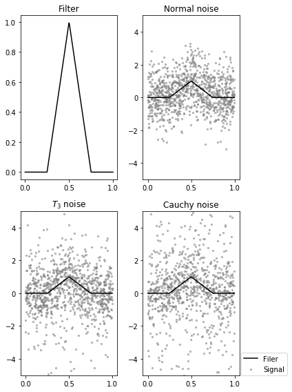
(a) Template $A$

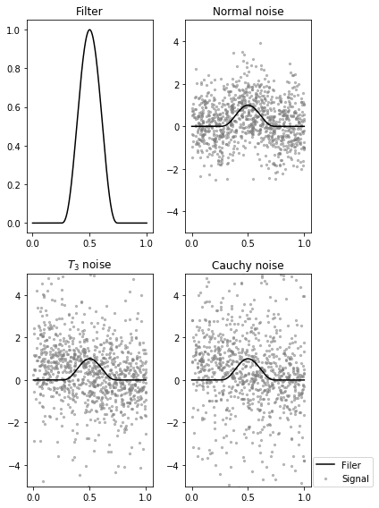
(b) Template $B$

Figure 2: Templates and noisy signals. Although the sample size is $n=10000$, for the sake of clarity, we only include $1000$ points and limit the range of the y-axis to $[-5,5]$.

We used a sample of size $n=10000$ and repeated each scenario (combination of template, noise distribution, and loss function) $200$ times. We show the mean of $|\sqrt{n}(\hat{\theta_{n}}-\theta^{*})|$ in Table 1. Box plots of estimation error $|\hat{\theta_{n}}-\theta^{*}|$ are shown in Figure 3 and Figure 4. The distribution of $\sqrt{n}(\hat{\theta_{n}}-\theta^{*})$ is plotted in Figure 5 and Figure 6 as an histogram overlaid with the Gaussian distribution predicted by our asymptotic calculations. Out of curiosity, we also looked at the setting where the noise is Cauchy and yet we use squared error as loss in Figure 7. The result of these experiments are by and large congruent with our theory. In particular, there is no noticeable difference between the two templates.

Template	Noise	Loss Function
		Squared error	Absolute-value	Huber	Tukey
Template $A$	Normal	0.2791	0.3705	0.2620	0.3301
	$T_{3}$	0.5168	0.3496	0.3634	0.5053
	Cauchy	28.2535	0.4355	0.5203	0.4113
Template $B$	Normal	0.2511	0.3326	0.2453	0.2918
	$T_{3}$	0.4524	0.3236	0.3293	0.3286
	Cauchy	48.2211	0.3958	0.3982	0.3462

Table 1: Mean of $|\sqrt{n}(\hat{\theta_{n}}-\theta^{*})|$ with $n=10000$ over $200$ repeats.

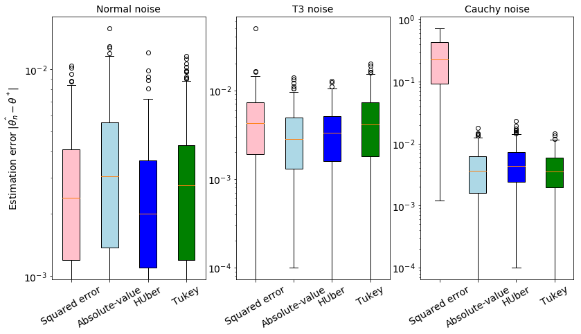
Figure 3: Box plot of estimation error $|\hat{\theta_{n}}-\theta^{*}|$ for Template $A$

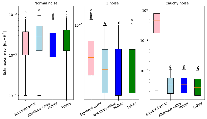
Figure 4: Box plot of estimation error $|\hat{\theta_{n}}-\theta^{*}|$ for Template $B$

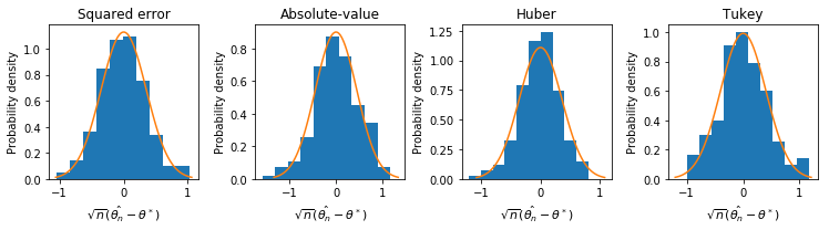
(a) Normal noise

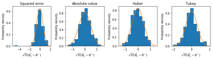
(b) $T_{3}$ noise

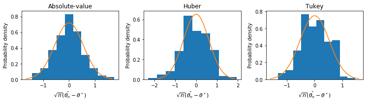
(c) Cauchy noise

Figure 5: Distribution under Template $A$. The histogram presents the distribution of $\sqrt{n}(\hat{\theta_{n}}-\theta^{*})$. The orange bell-shaped curve is the density of normal distribution predicted by the theory.

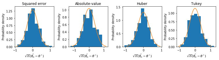
(a) Normal noise

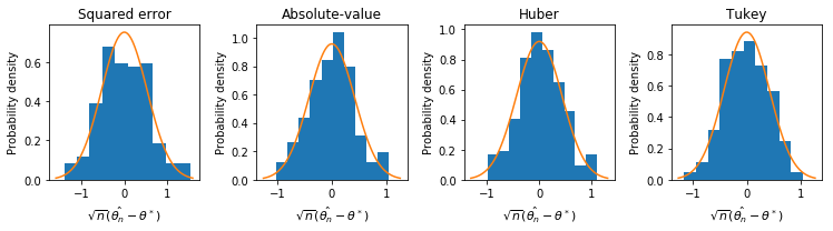
(b) $T_{3}$ noise

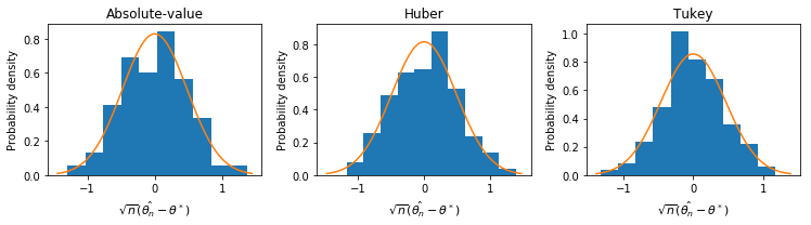
(c) Cauchy noise

Figure 6: Distribution under Template $B$. The histogram presents the distribution of $\sqrt{n}(\hat{\theta_{n}}-\theta^{*})$. The orange bell-shaped curve is the density of normal distribution predicted by the theory.

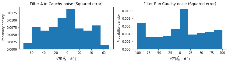
Figure 7: Distribution of $\sqrt{n}(\hat{\theta_{n}}-\theta^{*})$, for Templates $A$ and $B$, with squared error loss under the Cauchy distribution as noise distribution. Note that our theory is silent on this setting.

We also ran experiments with varying sample size $n$. We focused on Template $A$ with absolute-value loss and $T_{3}$ noise, to investigate the accuracy of the asymptotic distribution as $n$ increases. As sample size we used $n\in\{100,500,1000,5000,10000\}$. To have a finer sense of the accuracy, we used $1000$ repeats. We show the mean of $|\sqrt{n}(\hat{\theta_{n}}-\theta^{*})|$ in Table 2, the box plot of $|\hat{\theta_{n}}-\theta^{*}|$ in Figure 8, and the histogram of $\sqrt{n}(\hat{\theta_{n}}-\theta^{*})$ in Figure 9.

n	100	500	1000	5000	10000
Mean of $|\sqrt{n}(\hat{\theta_{n}}-\theta^{*})|$	0.5704	0.4286	0.4278	0.3766	0.3889

Table 2: Mean of $|\sqrt{n}(\hat{\theta_{n}}-\theta^{*})|$ for Template $A$ with absolute-value loss and $T_{3}$ noise based on $1000$ repeats.

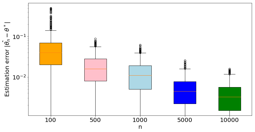
Figure 8: Box plot of the estimation error $|\hat{\theta_{n}}-\theta^{*}|$ for Template $A$ with absolute-value loss and $T_{3}$ noise based on $1000$ repeats.

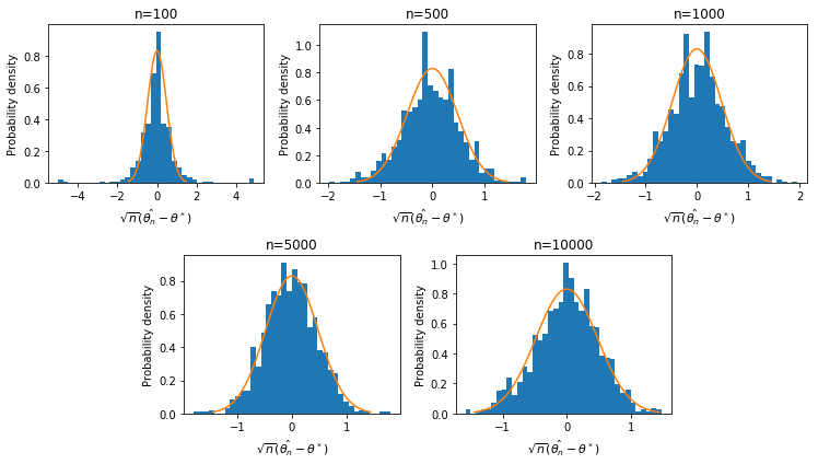
Figure 9: Distribution of $\sqrt{n}(\hat{\theta_{n}}-\theta^{*})$ for Template $A$ with absolute-value loss and $T_{3}$ noise based on $1000$ repeats.

In Figure 9, as $n\rightarrow\infty$, the distributions of $\sqrt{n}(\hat{\theta_{n}}-\theta^{*})$ approaches to the normal distribution shown in the theory. Figure 8 indicates estimation error $|\hat{\theta_{n}}-\theta^{*}|$ decreases as $n$ increases.

7.2 Non-smooth setting

We consider the following three filters:

$$\text{Template $C$: }\;\;f(x)=\begin{cases}1&0.25\leq x<0.75,\\ 0&\text{otherwise,}\end{cases}$$ (137)

$$\text{Template $D$: }\;\;f(x)=\begin{cases}1&0.2\leq x<0.4\;\;\text{or}\;\;0.6\leq x<0.8,\\ 0&\text{otherwise}\end{cases}$$ (138)

and

$$\text{Template $E$: }\;\;f(x)=\begin{cases}4x-1&0.25\leq x<0.5,\\ 0&\text{otherwise.}\end{cases}$$ (139)

Template $C$ is a piecewise constant function with two discontinuities. Template $D$ is another piecewise constant function with more discontinuities. Template $E$ is a half-triangle with one discontinuity. See Figure 10 for an illustration. Our theory predict that what matters is the number and size of the discontinuities.

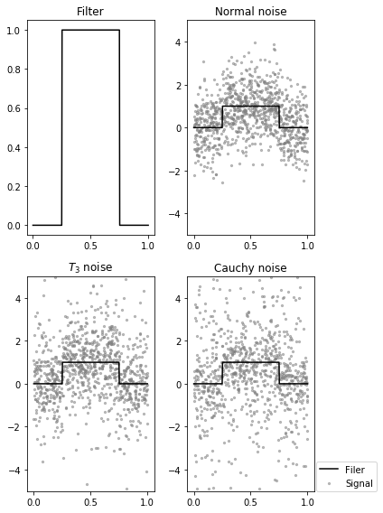
(a) Template $C$

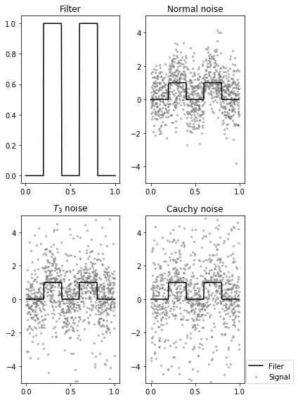
(b) Template $D$

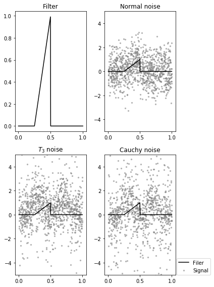
(c) Template $E$

Figure 10: Templates and noisy signals. Although the sample size is $n=10000$, for the sake of clarity, we only include $1000$ points and limit the range of the y-axis to $[-5,5]$.

We show the mean of $|n(\hat{\theta_{n}}-\theta^{*})|$ in Table 3, the estimation error $|\hat{\theta_{n}}-\theta^{*}|$ is shown as a box plot in Figures 11, 12, and 13, and the distribution of $n(\hat{\theta_{n}}-\theta^{*})$ is plotted in Figures 14, 15, and 16.

Template	Noise	Loss Function
		Squared error	Absolute-value	Huber	Tukey
Template $C$	Normal	1.876	1.849	1.868	2.120
	$T_{3}$	3.889	2.739	3.550	2.761
	Cauchy	2326.050	4.362	3.310	4.204
Template $D$	Normal	0.868	1.080	0.897	0.877
	$T_{3}$	1.802	1.220	1.344	1.813
	Cauchy	2766.000	2.278	2.078	1.862
Template $E$	Normal	3.498	3.798	3.414	4.008
	$T_{3}$	7.307	5.366	5.720	5.734
	Cauchy	4798.370	9.102	8.839	7.759

Table 3: Mean of $|n(\hat{\theta_{n}}-\theta^{*})|$ based on $200$ repeats.

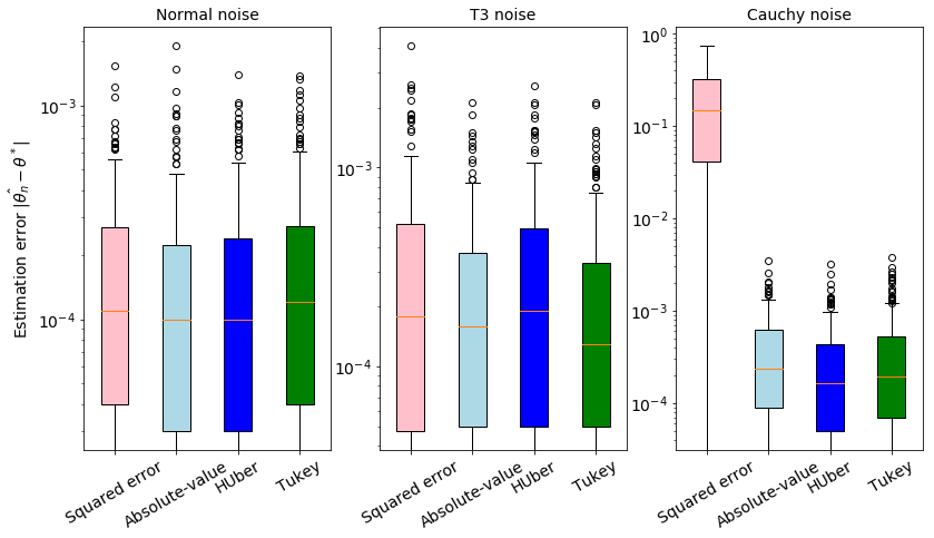
Figure 11: Box plot of estimation error $|\hat{\theta_{n}}-\theta^{*}|$ for Template $C$ based on $200$ repeats.

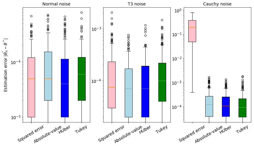
Figure 12: Box plot of estimation error $|\hat{\theta_{n}}-\theta^{*}|$ for Template $D$ based on $200$ repeats.

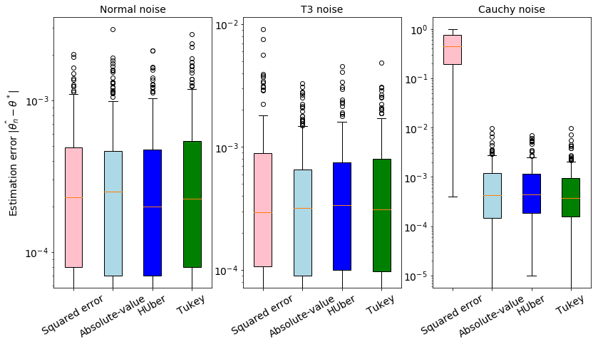
Figure 13: Box plot of estimation error $|\hat{\theta_{n}}-\theta^{*}|$ for Template $E$ based on $200$ repeats.

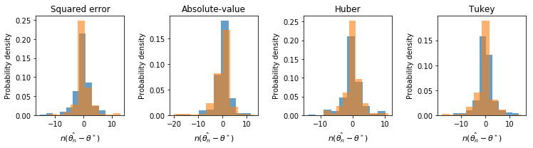
(a) Normal noise

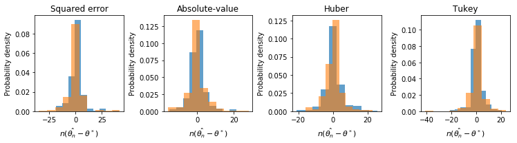
(b) $T_{3}$ noise

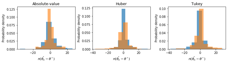
(c) Cauchy noise

Figure 14: The blue histogram represents the distribution of $n(\hat{\theta_{n}}-\theta^{*})$ for Template $C$. The orange histograms shows the simulated density of the midpoint of the minimizer interval of the marked Poisson process predicted by the theory. Based on $200$ repeats.

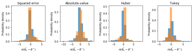
(a) Normal noise

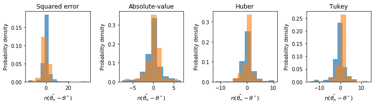
(b) $T_{3}$ noise

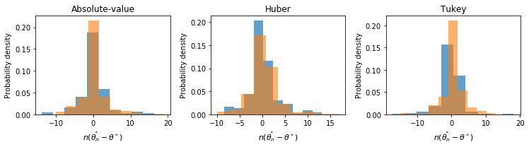
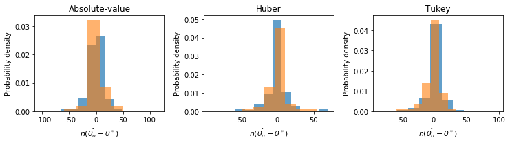
(c) Cauchy noise

Figure 15: The blue histogram represents the distribution of $n(\hat{\theta_{n}}-\theta^{*})$ for Template $D$. The orange histograms shows the simulated density of the midpoint of the minimizer interval of the marked Poisson process predicted by the theory. Based on $200$ repeats.

(a) Normal noise

(b) $T_{3}$ noise

(c) Cauchy noise

Figure 16: The blue histogram represents the distribution of $n(\hat{\theta_{n}}-\theta^{*})$ for Template $E$. The orange histograms shows the simulated density of the midpoint of the minimizer interval of the marked Poisson process predicted by the theory. Based on $200$ repeats.

We also ran some experiments with varying $n$ as before. We focused on Template E with the absolute-value loss under the $T_{3}$ noise distribution. The mean of $|n(\hat{\theta_{n}}-\theta^{*})|$ is reported in Table 4, a box plot of the estimation error $|\hat{\theta_{n}}-\theta^{*}|$ is given in Figure 17, and the distribution of $n(\hat{\theta_{n}}-\theta^{*})$ is plotted in Figure 18.

n	100	500	1000	5000	10000
Mean of $|n(\hat{\theta_{n}}-\theta^{*})|$	10.1872	5.0808	5.7420	5.7146	5.0682

Table 4: Mean of $|n(\hat{\theta_{n}}-\theta^{*})|$ for Template $E$ with absolute-value loss under $T_{3}$ noise based on $1000$ repeats.

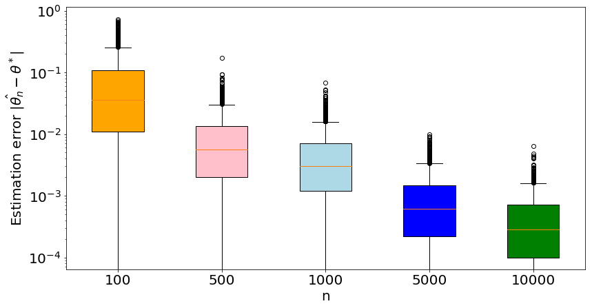
Figure 17: Box plot of estimation error $|\hat{\theta_{n}}-\theta^{*}|$ for Template $E$ with absolute-value loss under $T_{3}$ noise based on $1000$ repeats.

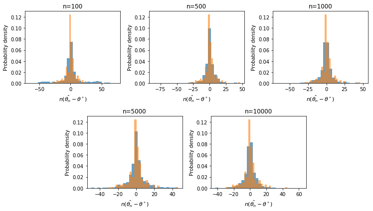
Figure 18: The blue histograms present the distribution of $n(\hat{\theta_{n}}-\theta^{*})$ for Template $E$ with absolute-value loss and $T_{3}$ noise. The orange histograms show the simulated density of marked Poisson process predicted by the theory. Based on $1000$ repeats.

Acknowledgments

We are particularly grateful to Lutz Dümbgen for providing some illuminating intuition for the change point setting where the template is discontinuous; to Jason Schweinsberg for clarifying the notion of weak convergence towards a Poisson process; and to Nicolas Verzelen for important pointers to the literature and for his general support throughout the writing of the paper. We are also thankful to Ioan Bejenaru, Richard Nickl, and Wenxin Zhou for helpful discussions and pointers.

Appendix A Miscellanea

A.1 Auxiliary results

Lemma A.1.

Suppose Assumptions 1, 3, and 4 are in place. Then, Asumption 5 is fulfilled if (i) the loss is strictly convex, or (ii) the noise distribution is unimodal and the loss is either Lipschitz or has a Lipschitz derivative and $\phi$ has finite first moment. Asumption 5 is also fulfilled for the Huber loss and the absolute-value loss if the noise distribution has a unique median.

Proof.

Assume $\theta^{*}=0$ without loss of generality. For $x$ and $y$ given, we let $z=y-f(x)$.

The function $\theta\mapsto m_{\theta}(x,y)$ is piecewise continuous under our assumptions. Moreover, it is dominated since, by the properties of ${\sf L}$,

$$m_{\theta}(x,y) ={\sf L}(y-f(x-\theta))$$

$$={\sf L}(y-f(x)+f(x)-f(x-\theta))$$

$$\leq{\sf L}(|y-f(x)|+|f(x)-f(x-\theta)|)$$

$$\leq\overline{m}(x,y):={\sf L}(|y-f(x)|+2|f|_{\infty}),$$

and $\operatorname{\mathbb{E}}[\overline{m}(X,Y)]<\infty$ by (10) and the fact that the loss is slowly increasing. Hence, $M$ is continuous by dominated convergence. In addition, by the fact that $f$ is compactly supported, $m_{\theta}(x,y)\to{\sf L}(y)$ when $\theta\to\pm\infty$, and so we also have $M(\theta)\to M(\infty):=\operatorname{\mathbb{E}}[{\sf L}(Y)]$ as $\theta\to\pm\infty$. We have

$$M(\theta)=\operatorname{\mathbb{E}}[{\sf L}(Z+f(X)-f(X-\theta))], M(\infty)=\operatorname{\mathbb{E}}[{\sf L}(Z+f(X))].$$

The identifiability condition in Asumption 1 implies that $\operatorname{\mathbb{P}}(f(X)-f(X-\theta)\neq 0)>0$ when $\theta\neq 0$ and $\operatorname{\mathbb{P}}(f(X)\neq 0)>0$, so by conditioning on $X$, taking into account that $X$ and $Z$ are independent, it suffices to prove that $g(a):=\operatorname{\mathbb{E}}[{\sf L}(Z+a)]$ achieves its minimum uniquely at $a=0$. Since $g$ is even, it suffices to prove that $g(a)>g(0)$ for any $a>0$.

Assume ${\sf L}$ is convex. Then

$$g(a)=\operatorname{\mathbb{E}}[{\sf L}(Z+a)] =\operatorname{\mathbb{E}}[{\sf L}(Z-a)]$$

$$=\operatorname{\mathbb{E}}[\tfrac{1}{2}{\sf L}(Z+a)+\tfrac{1}{2}{\sf L}(Z-a)]$$

$$\geq\operatorname{\mathbb{E}}[{\sf L}(Z)]=g(0),$$

where in the second equality we used the fact that the distribution of $Z$ is symmetric about 0 and that ${\sf L}$ is even, and in the inequality we used the fact that ${\sf L}$ is convex. That inequality is strict when the loss is strictly convex. This covers the squared error loss, for example.

For the Huber loss (5), the inequality is strict unless $Z-a\geq c$ or $Z+a\leq-c$ with probability 1, meaning that $\operatorname{\mathbb{P}}(Z\in[-a-c,a+c])=0$; for the absolute-value loss, the inequality is strict unless $\operatorname{sign}(Z-a)=\operatorname{sign}(Z+a)$ with probability 1, meaning that $\operatorname{\mathbb{P}}(Z\in[-a,a])=0$. In either case, this is only possible if the noise distribution does not put any mass in $[-a,a]$, which would then imply that any point in this entire interval is a median of the noise distribution.

Assume that the loss is Lipschitz. In that case, by dominated convergence, $g$ is differentiable with $g^{\prime}(a)=\operatorname{\mathbb{E}}[{\sf L}^{\prime}(Z+a)]$, and all we have to prove is that $g^{\prime}(a)\geq 0$ when the noise distribution is unimodal. (Recall that we work with $a>0$.) The uniqueness would then come from the fact that $g$ is not constant. We have

$$g^{\prime}(a) =\int_{-\infty}^{\infty}{\sf L}^{\prime}(z+a)\phi(z){\rm d}z$$

$$=\int_{0}^{\infty}{\sf L}^{\prime}(z)\big{\{}\phi(z-a)-\phi(z+a)\big{\}}{\rm d}z.$$

We claim that the integrand is non-negative. Indeed, ${\sf L}^{\prime}(z)\geq 0$ for $z\geq 0$ since ${\sf L}$ is non-decreasing away from the origin per Asumption 4. Also, using the fact that $\phi$ is non-increasing on $[0,\infty)$, we reason as follows: if $z\geq a$, then $z+a\geq z-a\geq 0$, implying $\phi(z+a)\leq\phi(z-a)$; and if $z\leq a$, then $a+z\geq a-z\geq 0$, implying $\phi(a+z)\leq\phi(a-z)$, in turn implying $\phi(z+a)\leq\phi(z-a)$ since $\phi$ is even. Our claim is thus established. This covers the Tukey loss, for example.

Assume that the loss has a Lipschitz derivative. In that case we can reduce this to the previous case by observing that $g$ above remains differentiable as long as $\phi$ has a finite first moment. Indeed,

$$\operatorname{\mathbb{E}}[|{\sf L}^{\prime}(Z+a)|]\leq\operatorname{\mathbb{E}}[|{\sf L}^{\prime\prime}|_{\infty}|Z+a|]\leq|{\sf L}^{\prime\prime}|_{\infty}(\operatorname{\mathbb{E}}[|Z|]+a)<\infty,$$ (140)

for all $a\geq 0$. ∎

Lemma A.2.

Suppose that, on the real line, $X_{1},\dots,X_{n}$ are iid from some density $\lambda$, and independently, that $A_{1},\dots,A_{n}$ are iid with distribution $\Psi$. Fix a finite subset $d_{1}<\cdots<d_{p}$ where $\lambda$ can be taken to be continuous. Define $W_{n,j}(t)=\sum_{i}\{d_{j}<X_{i}\leq d_{j}+t/n\}A_{i}$. Then $W_{n,j}$ converges weakly to the marked Poisson process with intensity $\lambda(d_{j})$ on the positive real line and mark distribution $\Psi$. Moreover, $W_{n,1},\dots,W_{n,p}$ are asymptotically independent.

Proof.

It is suffices to establish the statement on intervals. Without loss of generality, we consider the unit interval, so that we only consider $t\in[0,1]$. Everywhere, $n$ is large enough that $d_{j+1}-d_{j}>1/n$ for all $j$. This guarantees that, for any $t\in[0,1]$, the intervals $[d_{j},d_{j}+t/n]$ are disjoint. Let $\{A_{j,i}:i\geq 1,j=1,\dots,p\}$ be iid from $\Psi$. Then it’s easy to see that $W_{n,1},\dots,W_{n,p}$, jointly, have the same distribution as $\tilde{W}_{n,1},\dots,\tilde{W}_{n,p}$, where

$$\tilde{W}_{n,j}(t):=\sum_{i=1}^{N_{n,j}(t)}A_{j,i},\quad N_{n,j}(t):=\#\{i:d_{j}<X_{i}\leq d_{j}+t/n\}.$$ (141)

It is thus sufficient to show that $N_{n,j}$ converges weakly to the Poisson process with intensity $\lambda(d_{j})$ on the positive real line and that $N_{n,1},\dots,N_{n,p}$ are asymptotically independent. By (Billingsley, 1999, Th 12.6), it suffices to look at the finite-dimensional distributions. Therefore, fix $0\leq t_{1}<\cdots<t_{k}\leq 1$ and $\{n_{j,s}:j=1,\dots,p;s=1,\dots,k\}$ non-negative integers. Based on the ‘balls-in-bins’ dependency structure of these counts, we have

$$\operatorname{\mathbb{P}}\big{(}N_{n,j}(t_{s})\leq n_{j,s},\forall j\in[p],s\in[k]\big{)}$$ (142)

$$=\operatorname{\mathbb{P}}\big{(}N_{n,1}(t_{s})\leq n_{1,s},\forall s\in[k]\big{)}$$ (143)

$$\quad\times\operatorname{\mathbb{P}}\big{(}N_{n,2}(t_{s})\leq n_{2,s},\forall s\in[k]\mid N_{n,1}(t_{k})\leq n_{1,k}\big{)}$$ (144)

$$\quad\quad\times\cdots$$ (145)

$$\quad\quad\quad\times\operatorname{\mathbb{P}}\big{(}N_{n,p}(t_{s})\leq n_{p,s},\forall s\in[k]\mid N_{n,1}(t_{k})\leq n_{1,k},\dots,N_{n,p-1}(t_{k})\leq n_{p-1,k}\big{)},$$ (146)

with

$$\operatorname{\mathbb{P}}\big{(}N_{n,j}(t_{s})\leq n_{j,s},\forall s\in[k]\mid N_{n,1}(t_{k})\leq n_{1,k},\dots,N_{n,j-1}(t_{k})\leq n_{j-1,k}\big{)}$$

$$\begin{cases}\geq\operatorname{\mathbb{P}}\big{(}N_{n,j}(t_{s})\leq n_{j,s},\forall s\in[k]\big{)}\\ \leq\operatorname{\mathbb{P}}\big{(}N_{n-r_{j},j}(t_{s})\leq n_{j,s},\forall s\in[k]\big{)},\quad r_{j}:=n_{1,k}+\cdots+n_{j-1,k}.\end{cases}$$

Note that $r_{1},\dots,r_{p}$ are all fixed, and it’s easy to convince oneself that it suffices at this point to show that, for each $j$,

$$\operatorname{\mathbb{P}}\big{(}N_{n,j}(t_{s})\leq n_{j,s},\forall s\in[k]\big{)}\xrightarrow{n\to\infty}\operatorname{\mathbb{P}}\big{(}N_{j}(t_{s})\leq n_{j,s},\forall s\in[k]\big{)},$$ (147)

were $N_{j}$ is a Poisson process with intensity $\lambda(d_{j})$ on the positive real line, in other words, that $N_{n,j}$ converges weakly to $N_{j}$. We do so by looking at the probability mass function instead of the cumulative distribution function. With $t_{1}<\cdots<t_{k}$ and $\{n_{j,s}\}$ generic, we have

$$\operatorname{\mathbb{P}}\big{(}N_{n,j}(t_{1})=n_{j,1},\dots,N_{n,j}(t_{k})=n_{j,k}\big{)}$$

$$=\operatorname{\mathbb{P}}\big{(}N_{n,j}(t_{1})=n_{j,1},N_{n,j}(t_{2})-N_{n,j}(t_{1})=n_{j,2}-n_{j,1},\dots,N_{n,j}(t_{k})-N_{n,j}(t_{k-1})=n_{j,k}-n_{j,k-1}\big{)}$$

$$\sim\operatorname{\mathbb{P}}\big{(}N_{n,j}(t_{1})=n_{j,1}\big{)}\times\operatorname{\mathbb{P}}\big{(}N_{n,j}(t_{2})-N_{n,j}(t_{1})=n_{j,2}-n_{j,1}\big{)}$$

$$\quad\quad\quad\quad\times\cdots\times\operatorname{\mathbb{P}}\big{(}N_{n,j}(t_{k})-N_{n,j}(t_{k-1})=n_{j,k}-n_{j,k-1}\big{)},\quad\text{as }n\to\infty,$$

where the approximation follows the same arguments used above to prove the asymptotic independence of the various count processes. We then conclude with the fact that, for any $m\geq 0$ integer,

$$\operatorname{\mathbb{P}}\big{(}N_{n,j}(t_{s})-N_{n,j}(t_{s-1})=m\big{)} =\#\{i:d_{j}+t_{s-1}/n<X_{i}\leq d_{j}+t_{s}/n\}$$

$$\xrightarrow{n\to\infty}\lambda(d_{j})(t_{s}-t_{s-1})=\operatorname{\mathbb{P}}\big{(}N_{j}(t_{s})-N_{j}(t_{s-1})=m\big{)},$$

using the fact that $\lambda$ is continuous at $d_{j}$. ∎

Lemma A.3.

Consider the setting of Section 5.2. Assume in addition that $\operatorname{\mathbb{E}}[{\sf L}(Z)]<{\sf L}(\infty)$ and that $\operatorname{\mathbb{E}}[{\sf L}(Z)]<\operatorname{\mathbb{E}}[{\sf L}(Z+a)]$ for all $a\neq 0$. Then there is a compact subset $\Theta_{0}\subset\Theta$ of the form $[-B,B]\times[-B,B]\times[1/B,B]$ for some $B\geq 1$, such that, with probability tending to 1, any minimizer $\hat{\theta}_{n}$ of $\widehat{M}_{n}$ is in $\Theta_{0}$.

Proof.

Let $a=\inf\{x:f(x)>0\}$ and $b=\sup\{x:f(x)>0\}$, and assume that $\lambda$ is supported on $[-c,c]$. Since we know that $f_{\theta^{*}}$ has support contained within the support of $\lambda$, we can restrict attention to those $\theta$ such that $f_{\theta}$ has support contained within the support of $\lambda$, which is equivalent to $\xi$ and $\nu$ satisfying $\xi+a\nu\geq-c$ and $\xi+b\nu\leq c$. Note that this implies that $-c|b+a|/(b-a)\leq\xi\leq c|b+a|/(b-a)$ and $\nu\leq 2c/(b-a)$.

We now show that there is $\nu_{0}>0$ such that, if $\nu\leq\nu_{0}$, then $\widehat{M}_{n}(\beta,\xi,\nu)$ is, asymptotically, bounded away (and above) from $\widehat{M}_{n}(\theta^{*})$, regardless of $\beta$ and $\xi$. Henceforth, we assume without loss of generality that $\theta^{*}=(1,0,1)$.

On the one hand, by the law of large numbers, in probability as $n\to\infty$,

$$\widehat{M}_{n}(\theta^{*})\to M(\theta^{*})=\operatorname{\mathbb{E}}[{\sf L}(Z)].$$ (148)

On the other hand,

$$\inf_{\beta,\xi,\nu\leq\nu_{0}}\widehat{M}_{n}(\beta,\xi,\nu) =\inf_{\beta,\xi,\nu\leq\nu_{0}}\frac{1}{n}\sum_{i}{\sf L}\big{(}Z_{i}+f(X_{i})-\beta f((X_{i}-\xi)/\nu)\big{)}$$ (149)

$$\geq\inf_{\beta,\xi,\nu\leq\nu_{0}}\frac{1}{n}\sum_{i}{\sf L}\big{(}Z_{i}+f(X_{i}))\mathbb{I}{\{X_{i}\notin\xi\pm\nu K\}}$$ (150)

$$=\inf_{|I|\leq 2\nu_{0}K}\frac{1}{n}\sum_{i}{\sf L}\big{(}Z_{i}+f(X_{i}))\mathbb{I}{\{X_{i}\notin I\}},$$ (151)

where $I$ above is a closed interval of length $|I|$. The inequality relies on the fact that $\beta f((x-\xi)/\nu)=0$ when $x\notin\xi\pm\nu K$ and the fact that the loss function is non-negative. Now,

$$\frac{1}{n}\sum_{i}{\sf L}\big{(}Z_{i}+f(X_{i}))\mathbb{I}{\{X_{i}\notin I\}}=\frac{1}{n}\sum_{i}g_{I}(X_{i},Z_{i}),\quad g_{I}(x,z):={\sf L}\big{(}z+f(x))\mathbb{I}{\{x\notin I\}},$$ (152)

and the class of functions $\{g_{I}:|I|\leq 2\nu_{0}K\}$ is clearly Glivenko–Cantelli. Hence,

$$\inf_{|I|\leq 2\nu_{0}K}\frac{1}{n}\sum_{i}{\sf L}\big{(}Z_{i}+f(X_{i}))\mathbb{I}{\{X_{i}\notin I\}}\xrightarrow{n\to\infty}\inf_{|I|\leq 2\nu_{0}K}\operatorname{\mathbb{E}}[{\sf L}\big{(}Z+f(X))\mathbb{I}{\{X\notin I\}}].$$ (153)

In turn, by dominated convergence, as $\nu_{0}\to 0$, the last expression converges to $\operatorname{\mathbb{E}}[{\sf L}(Z+f(X))]$, which is strictly larger than $\operatorname{\mathbb{E}}[{\sf L}(Z)]$ by (the equivalent of) Asumption 5. In particular, if $\nu_{0}$ is so small that the last infimum is $>\operatorname{\mathbb{E}}[{\sf L}(Z)]$, we guarantee that, with probability tending to 1, $\hat{\nu}_{n}\geq\nu_{0}$.

So far, we showed that we can restrict $(\xi,\nu)$ in order for $f_{\theta}$ to have support inside that of $\lambda$, and that we may add a lower bound on $\nu$ (away from $0$). It remains to show that, under these conditions, we may also add a bound on $|\beta|$. Fix $\varepsilon>0$ and define $S_{\varepsilon}=\{x:|f(x)|>\varepsilon\}$. Then, with the infimum over $\xi$ and $\nu$ restricted as described above, for $\beta_{0}>0$ and $z_{0}>0$, we have

$$\inf_{|\beta|\geq\beta_{0},\xi,\nu}\widehat{M}_{n}(\beta,\xi,\nu)$$

$$\geq\inf_{|\beta|\geq\beta_{0},\xi,\nu}\quad\frac{1}{n}\sum_{i}\inf_{|a_{i}|\geq\varepsilon}{\sf L}\big{(}Z_{i}+f(X_{i})-\beta a_{i}\big{)}\mathbb{I}{\{X_{i}\in\xi+\nu S_{\varepsilon}\}}+\frac{1}{n}\sum_{i}{\sf L}\big{(}Z_{i}+f(X_{i})\big{)}\mathbb{I}{\{X_{i}\notin\xi+\nu S_{0}\}}$$

$$\geq\inf_{\xi,\nu}\quad\frac{1}{n}\sum_{i}{\sf L}((\beta_{0}\varepsilon-Z_{i}-f(X_{i}))_{+})\mathbb{I}{\{X_{i}\in\xi+\nu S_{\varepsilon}\}}+\frac{1}{n}\sum_{i}{\sf L}\big{(}Z_{i}+f(X_{i})\big{)}\mathbb{I}{\{X_{i}\notin\xi+\nu S_{0}\}}$$

$$\xrightarrow{n\to\infty}\inf_{\xi,\nu}\quad\operatorname{\mathbb{E}}[{\sf L}((\beta_{0}\varepsilon-Z-f(X))_{+})\mathbb{I}{\{X\in\xi+\nu S_{\varepsilon}\}}]+\operatorname{\mathbb{E}}[{\sf L}(Z+f(X))\mathbb{I}{\{X\notin\xi+\nu S_{0}\}}]$$

$$\xrightarrow{\beta_{0}\to\infty}\inf_{\xi,\nu}\quad{\sf L}(\infty)\operatorname{\mathbb{P}}(X\in\xi+\nu S_{\varepsilon})+\operatorname{\mathbb{E}}[{\sf L}(Z+f(X))\mathbb{I}{\{X\notin\xi+\nu S_{0}\}}]$$

$$\xrightarrow{\varepsilon\to 0}\inf_{\xi,\nu}\quad{\sf L}(\infty)\operatorname{\mathbb{P}}(X\in\xi+\nu S_{0})+\operatorname{\mathbb{E}}[{\sf L}(Z+f(X))\mathbb{I}{\{X\notin\xi+\nu S_{0}\}}].$$

The first limit uses a uniform law of large numbers as we did above, only here it is based on the fact that the collection of sets of the form $\xi+\nu S_{\varepsilon}$, as $\xi$ and $\nu$ vary as they do here, has finite VC dimension, and similarly for the collection of sets of the form $\xi+\nu S_{0}$. We compare the last expression with $M(\theta^{*})$ to get

$${\sf L}(\infty)\operatorname{\mathbb{P}}(X\in\xi+\nu S_{0})+\operatorname{\mathbb{E}}[{\sf L}(Z+f(X))\mathbb{I}{\{X\notin\xi+\nu S_{0}\}}]-M(\theta^{*})$$ (154)

$$=({\sf L}(\infty)-\operatorname{\mathbb{E}}[{\sf L}(Z)])\operatorname{\mathbb{P}}(X\in\xi+\nu S_{0})+\operatorname{\mathbb{E}}[\varphi(f(X))\mathbb{I}{\{X\notin\xi+\nu S_{0}\}}]=:Q(\xi,\nu),$$ (155)

where $\varphi(a):=\operatorname{\mathbb{E}}[{\sf L}(Z+a)]-\operatorname{\mathbb{E}}[{\sf L}(Z)]$. By assumption, ${\sf L}(\infty)-\operatorname{\mathbb{E}}[{\sf L}(Z)]>0$ and $\varphi(a)>0$ when $a\neq 0$, so that $Q(\xi,\nu)=0$ if and only if $\operatorname{\mathbb{P}}(X\in\xi+\nu S_{0})=0$ and $\operatorname{\mathbb{P}}(X\notin\xi+\nu S_{0},X\in S_{0})=0$, which together imply that $\operatorname{\mathbb{P}}(X\in S_{0})=0$, which would contradict the fact that $f\nequiv 0$ on the support of $\lambda$. Hence, $Q(\xi,\nu)>0$, and since $Q$ is continuous by dominated convergence, and $(\xi,\nu)$ is in a compact set, we have that $\inf_{\xi,\nu}Q(\xi,\nu)>0$. All in all, we are able to conclude that there is $\beta_{0}>0$ such that, with probability tending to 1, $|\hat{\beta}_{n}|\leq\beta_{0}$. And this is the only thing that was left to prove to establish the lemma. ∎

References

• Arias-Castro et al. (2011) Arias-Castro, E., E. J. Candès, and A. Durand (2011). Detection of an anomalous cluster in a network. The Annals of Statistics 39(1), 278–304.
• Arias-Castro et al. (2018) Arias-Castro, E., R. M. Castro, E. Tánczos, and M. Wang (2018). Distribution-free detection of structured anomalies: Permutation and rank-based scans. Journal of the American Statistical Association 113(522), 789–801.
• Arias-Castro et al. (2005) Arias-Castro, E., D. L. Donoho, and X. Huo (2005). Near-optimal detection of geometric objects by fast multiscale methods. IEEE Transactions on Information Theory 51(7), 2402–2425.
• Bai (1997) Bai, J. (1997). Estimation of a change point in multiple regression models. Review of Economics and Statistics 79(4), 551–563.
• Basseville and Nikiforov (1993) Basseville, M. and I. V. Nikiforov (1993). Detection of abrupt changes: theory and application, Volume 104. Englewood Cliffs, New Jersey: Prentice Hall.
• Belongie et al. (2002) Belongie, S., J. Malik, and J. Puzicha (2002). Shape matching and object recognition using shape contexts. IEEE Transactions on Pattern Analysis and Machine Intelligence 24(4), 509–522.
• Bickel et al. (1998) Bickel, P., C. Klaassen, Y. Ritov, and J. Wellner (1998). Efficient and adaptive estimation for semiparametric models. Springer.
• Bigot et al. (2009) Bigot, J., F. Gamboa, and M. Vimond (2009). Estimation of translation, rotation, and scaling between noisy images using the Fourier–Mellin transform. SIAM Journal on Imaging Sciences 2(2), 614–645.
• Billingsley (1999) Billingsley, P. (1999). Convergence of probability measures. John wiley & Sons.
• Boutsikas and Koutras (2006) Boutsikas, M. V. and M. V. Koutras (2006). On the asymptotic distribution of the discrete scan statistic. Journal of Applied Probability 43(4), 1137–1154.
• Brodsky and Darkhovsky (2013) Brodsky, E. and B. S. Darkhovsky (2013). Nonparametric methods in change point problems, Volume 243. Springer Science$+$Business Media.
• Brunelli (2009) Brunelli, R. (2009). Template matching techniques in computer vision: theory and practice. John Wiley & Sons.
• Chen and Gupta (2011) Chen, J. and A. K. Gupta (2011). Parametric statistical change point analysis: with applications to genetics, medicine, and finance. Springer Science$+$Business Media.
• Collier and Dalalyan (2012) Collier, O. and A. S. Dalalyan (2012). Minimax hypothesis testing for curve registration. Electronic Journal of Statistics 6, 1129–1154.
• Collier and Dalalyan (2015) Collier, O. and A. S. Dalalyan (2015). Curve registration by nonparametric goodness-of-fit testing. Journal of Statistical Planning and Inference 162, 20–42.
• Csörgö and Horváth (1997) Csörgö, M. and L. Horváth (1997). Limit theorems in change-point analysis. John Wiley & Sons Inc.
• Desolneux et al. (2003) Desolneux, A., L. Moisan, and J.-M. Morel (2003). Maximal meaningful events and applications to image analysis. The Annals of Statistics 31(6), 1822–1851.
• Döring (2011) Döring, M. (2011). Convergence in distribution of multiple change point estimators. Journal of Statistical Planning and Inference 141(7), 2238–2248.
• Dudley (1967) Dudley, R. M. (1967). The sizes of compact subsets of Hilbert space and continuity of Gaussian processes. Journal of Functional Analysis 1(3), 290–330.
• Dümbgen (1991) Dümbgen, L. (1991). The asymptotic behavior of some nonparametric change-point estimators. The Annals of Statistics 19(3), 1471–1495.
• Ferger (1994) Ferger, D. (1994). Change-point estimators in case of small disorders. Journal of Statistical Planning and Inference 40(1), 33–49.
• Ferger (2001) Ferger, D. (2001). Exponential and polynomial tailbounds for change-point estimators. Journal of Statistical Planning and Inference 92(1-2), 73–109.
• Ferger (2004) Ferger, D. (2004). A continuous mapping theorem for the argmax-functional in the non-unique case. Statistica Neerlandica 58(1), 83–96.
• Frick et al. (2014) Frick, K., A. Munk, and H. Sieling (2014). Multiscale change point inference. Journal of the Royal Statistical Society - Series B: Statistical Methodology 76(3), 495–580.
• Gamboa et al. (2007) Gamboa, F., J.-M. Loubès, and E. Maza (2007). Semi-parametric estimation of shifts. Electronic Journal of Statistics 1, 616–640.
• Glaz and Balakrishnan (2012) Glaz, J. and N. Balakrishnan (2012). Scan statistics and applications. Springer Science$+$Business Media.
• Glaz et al. (2001) Glaz, J., J. Naus, and S. Wallenstein (2001). Scan statistics. Springer.
• Glaz et al. (2009) Glaz, J., V. Pozdnyakov, and S. Wallenstein (2009). Scan statistics: methods and applications. Springer Science$+$Business Media.
• Glaz and Zhang (2004) Glaz, J. and Z. Zhang (2004). Multiple window discrete scan statistics. Journal of Applied Statistics 31(8), 967–980.
• Haiman and Preda (2006) Haiman, G. and C. Preda (2006). Estimation for the distribution of two-dimensional discrete scan statistics. Methodology and Computing in Applied Probability 8(3), 373–382.
• Hajnal and Hill (2001) Hajnal, J. V. and D. L. Hill (2001). Medical image registration. CRC press.
• Hall and Jin (2010) Hall, P. and J. Jin (2010). Innovated higher criticism for detecting sparse signals in correlated noise. The Annals of Statistics 38(3), 1686–1732.
• Härdle and Marron (1990) Härdle, W. and J. Marron (1990). Semiparametric comparison of regression curves. The Annals of Statistics 18(1), 63–89.
• He and Severini (2010) He, H. and T. A. Severini (2010). Asymptotic properties of maximum likelihood estimators in models with multiple change points. Bernoulli 16(3), 759–779.
• Hinkley (1970) Hinkley, D. (1970). Inference about the change-point in a sequence of random variables. Biometrika 57(1), 1–17.
• Hjelmås and Low (2001) Hjelmås, E. and B. K. Low (2001). Face detection: A survey. Computer Vision and Image Understanding 83, 236–274.
• Jeng et al. (2010) Jeng, X. J., T. T. Cai, and H. Li (2010). Optimal sparse segment identification with application in copy number variation analysis. Journal of the American Statistical Association 105(491), 1156–1166.
• Jiang (2002) Jiang, T. (2002). Maxima of partial sums indexed by geometrical structures. The Annals of Probability 30(4), 1854–1892.
• Kabluchko (2011) Kabluchko, Z. (2011). Extremes of the standardized Gaussian noise. Stochastic Processes and their Applications 121(3), 515–533.
• Kim and Pollard (1990) Kim, J. and D. Pollard (1990). Cube root asymptotics. The Annals of Statistics 18(1), 191–219.
• Kneip and Engel (1995) Kneip, A. and J. Engel (1995). Model estimation in nonlinear regression under shape invariance. The Annals of Statistics 23(2), 551–570.
• Kneip and Gasser (1988) Kneip, A. and T. Gasser (1988). Convergence and consistency results for self-modeling nonlinear regression. The Annals of Statistics 16(1), 82–112.
• Kneip and Gasser (1992) Kneip, A. and T. Gasser (1992). Statistical tools to analyze data representing a sample of curves. The Annals of Statistics 20(3), 1266–1305.
• König et al. (2020) König, C., A. Munk, and F. Werner (2020). Multidimensional multiscale scanning in exponential families: Limit theory and statistical consequences. The Annals of Statistics 48(2), 655–678.
• Korostelev (1988) Korostelev, A. (1988). On minimax estimation of a discontinuous signal. Theory of Probability & Its Applications 32(4), 727–730.
• Kosorok (2008) Kosorok, M. R. (2008). Introduction to empirical processes and semiparametric inference. Springer Science+Business Media.
• Kou (2017) Kou, J. (2017). Identifying the support of rectangular signals in Gaussian noise. arXiv preprint arXiv:1703.06226.
• Lan et al. (2009) Lan, Y., M. Banerjee, and G. Michailidis (2009). Change-point estimation under adaptive sampling. The Annals of Statistics 37(4), 1752–1791.
• Lawton et al. (1972) Lawton, W., E. Sylvestre, and M. Maggio (1972). Self modeling nonlinear regression. Technometrics 14(3), 513–532.
• Lehmann and Romano (2005) Lehmann, E. L. and J. P. Romano (2005). Testing statistical hypotheses. Springer Science$+$Business Media.
• Lowe (1999) Lowe, D. G. (1999). Object recognition from local scale-invariant features. In International Conference on Computer Vision, Volume 2, pp. 1150–1157. IEEE.
• Mauer (2018) Mauer, R. (2018). Least squares estimation in multiple change-point models. Ph. D. thesis, Technische Universität Dresden.
• Naus and Wallenstein (2004) Naus, J. I. and S. Wallenstein (2004). Multiple window and cluster size scan procedures. Methodology and Computing in Applied Probability 6(4), 389–400.
• Perry et al. (2019) Perry, A., J. Weed, A. S. Bandeira, P. Rigollet, and A. Singer (2019). The sample complexity of multireference alignment. SIAM Journal on Mathematics of Data Science 1(3), 497–517.
• Perry et al. (2018) Perry, A., A. S. Wein, A. S. Bandeira, and A. Moitra (2018). Message-passing algorithms for synchronization problems over compact groups. Communications on Pure and Applied Mathematics 71(11), 2275–2322.
• Pozdnyakov et al. (2005) Pozdnyakov, V., J. Glaz, M. Kulldorff, and J. M. Steele (2005). A martingale approach to scan statistics. Annals of the Institute of Statistical Mathematics 57(1), 21–37.
• Proksch et al. (2018) Proksch, K., F. Werner, and A. Munk (2018). Multiscale scanning in inverse problems. The Annals of Statistics 46(6B), 3569–3602.
• Seijo and Sen (2011) Seijo, E. and B. Sen (2011). Change-point in stochastic design regression and the bootstrap. The Annals of Statistics 39(3), 1580–1607.
• Serre et al. (2005) Serre, T., L. Wolf, and T. Poggio (2005). Object recognition with features inspired by visual cortex. In 2005 IEEE Computer Society Conference on Computer Vision and Pattern Recognition (CVPR’05), Volume 2, pp.  994–1000. IEEE.
• Shao (1995) Shao, Q. M. (1995). On a conjecture of révész. Proceedings of the American Mathematical Society 123(2), 575–582.
• Sharpnack and Arias-Castro (2016) Sharpnack, J. and E. Arias-Castro (2016). Exact asymptotics for the scan statistic and fast alternatives. Electronic Journal of Statistics 10(2), 2641–2684.
• Siegmund (2013) Siegmund, D. (2013). Sequential analysis: tests and confidence intervals. Springer Science+Business Media.
• Siegmund and Venkatraman (1995) Siegmund, D. and E. S. Venkatraman (1995). Using the generalized likelihood ratio statistic for sequential detection of a change-point. The Annals of Statistics 23(1), 255–271.
• Sotiras et al. (2013) Sotiras, A., C. Davatzikos, and N. Paragios (2013). Deformable medical image registration: A survey. IEEE Transactions on Medical imaging 32(7), 1153–1190.
• Talagrand (1996) Talagrand, M. (1996). New concentration inequalities in product spaces. Inventiones Mathematicae 126(3), 505–563.
• Trigano et al. (2011) Trigano, T., U. Isserles, and Y. Ritov (2011). Semiparametric curve alignment and shift density estimation for biological data. IEEE Transactions on Signal Processing 59(5), 1970–1984.
• Truong et al. (2020) Truong, C., L. Oudre, and N. Vayatis (2020). Selective review of offline change point detection methods. Signal Processing 167, 107299.
• Tsybakov (2009) Tsybakov, A. B. (2009). Introduction to nonparametric estimation. Springer Science$+$Business Media.
• Turin (1960) Turin, G. (1960). An introduction to matched filters. IRE Transactions on Information Theory 6(3), 311–329.
• van der Vaart (1998) van der Vaart, A. W. (1998). Asymptotic statistics. Cambridge University Press.
• van der Vaart and Wellner (1996) van der Vaart, A. W. and J. A. Wellner (1996). Weak convergence and empirical processes with applications to statistics. Springer.
• Vimond (2010) Vimond, M. (2010). Efficient estimation for a subclass of shape invariant models. The Annals of Statistics 38(3), 1885–1912.
• Walther (2010) Walther, G. (2010). Optimal and fast detection of spatial clusters with scan statistics. The Annals of Statistics 38(2), 1010–1033.
• Wang and Gasser (1999) Wang, K. and T. Gasser (1999). Synchronizing sample curves nonparametrically. The Annals of Statistics 27(2), 439–460.
• Wang and Singer (2013) Wang, L. and A. Singer (2013). Exact and stable recovery of rotations for robust synchronization. Information and Inference: A Journal of the IMA 2(2), 145–193.
• Wang and Glaz (2014) Wang, X. and J. Glaz (2014). Variable window scan statistics for normal data. Communications in Statistics - Theory and Methods 43(10-12), 2489–2504.
• Yao and Au (1989) Yao, Y.-C. and S.-T. Au (1989). Least-squares estimation of a step function. Sankhyā: The Indian Journal of Statistics, Series A 51(3), 370–381.
• Zitova and Flusser (2003) Zitova, B. and J. Flusser (2003). Image registration methods: a survey. Image and Vision Computing 21(11), 977–1000.