∎
e1e-mail: nivaldolemos@id.uff.br \thankstexte2e-mail: reboucas.marcelo@gmail.com
Inquiring electromagnetic quantum fluctuations about the orientability of space
Abstract
Orientability is an important global topological property of spacetime manifolds. It is often assumed that a test for spatial orientability requires a global journey across the whole space to check for orientation-reversing paths. Since such a global expedition is not feasible, theoretical arguments that combine universality of physical experiments with local arrow of time, CP violation and CPT invariance are usually offered to support the choosing of time- and space-orientable spacetime manifolds. Another theoretical argument also offered to support this choice comes from the impossibility of having globally defined spinor fields on non-orientable spacetime manifolds. In this paper, we argue that it is possible to locally access spatial orientability of Minkowski empty spacetime through physical effects involving quantum vacuum electromagnetic fluctuations. We study the motions of a charged particle and a point electric dipole subject to these electromagnetic fluctuations in Minkowski spacetime with orientable and non-orientable spatial topologies. We derive analytic expressions for a statistical orientability indicator for both of these point-like particles in two inequivalent spatially flat topologies. For the charged particle, we show that it is possible to distinguish the orientable from the non-orientable topology by contrasting the time evolution of the orientability indicators. This result reveals that it is possible to access orientability through electromagnetic quantum vacuum fluctuations. However, the answer to the central question of the paper, namely how to locally probe the orientability of Minkowski space intrinsically, comes about only in the study of the motions of an electric dipole. For this point-like particle, we find that a characteristic inversion pattern exhibited by the curves of the orientability statistical indicator is a signature of non-orientability. This result makes it clear that it is possible to locally unveil spatial non-orientability through the inversion pattern of curves of our orientability indicator for a point electric dipole under quantum vacuum electromagnetic fluctuations. Our findings might open the way to a conceivable experiment involving quantum vacuum electromagnetic fluctuations to locally probe the spatial orientability of Minkowski empty spacetime.
Keywords:
Topology of Minkowski space Orientability of Minkowsk space Quantum fluctuations of electromagnetic field Motion of charged particle and dipole under electromagnetic fluctuationspacs:
03.70.+k 05.40.Jc 42.50.Lc 04.20.Gz 98.80.Jk 98.80.Cq1 Introduction
The Universe is modeled as a four-dimensional differentiable manifold, which is a topological space with an additional differential structure that permits to locally define connections, metric and curvature with which the gravitation theories are formulated. Geometry is a local attribute that brings about curvature, whereas topology is a global feature of a manifold related, for example, to compactness and orientability. Geometry constrains but does not specify the topology. So, topologically different manifolds can have a given geometry.111 Despite our present-day inability to predict the spatial topology of the Universe from a fundamental theory, one should be able to probe it through cosmic microwave background radiation (CMBR) or (and) stochastic primordial gravitational waves CosmTopReviews ; Reboucas2020 , which should follow some basic detectability conditions TopDetec . For recent topological constraints from CMBR data we refer the reader to Refs. Vaudrevange-etal-12 ; Planck-2013-XXVI ; Planck-2015-XVIII . For some limits on the circles-in-the-sky method designed for searches of cosmic topology through CMBR see Ref. Gomero-Mota-Reboucas-2016 .
Since topology antecedes geometry, it is important to determine whether, how and to what extent physical phenomena depend upon or are somehow affected, induced, triggered, or even driven by a nontrivial topology. The net role played by the spatial topology is more clearly ascertained in the static spatially flat Friedmann-Lemaître-Robertson-Walker spacetime, whose dynamical degrees of freedom are frozen. Thus, in this work we focus on Minkowski spacetime, whose spatial geometry is Euclidean.
Although the topology of the spatial section, , of Minkowski spacetime, , is usually taken to be the simply-connected Euclidean space , it is a mathematical fact that it can also be any one of the possible topologically distinct quotient (multiply-connected) manifolds , where is a discrete group of isometries or holonomies acting freely on the covering space Wolf67 ; Thurston . The action of tiles or tessellates the covering manifold into identical domains or cells which are copies of what is known as fundamental polyhedron (FP) or fundamental cell or domain (FC or FD). On the covering manifold , the multiple connectedness of is taken into account by imposing periodic boundary conditions (repeated cells) that are determined by the action of the group of discrete isometries on the covering space .
In a manifold with periodic boundary conditions only certain modes of fields can exist. Thus, a nontrivial topology may leave its mark on the expectation values of local physical quantities. A case in point is the Casimir effect of topological origin dhi79 ; Dowker-Critchley-1976 ; st06 ; MD-2007 ; DHO-2002 ; DHO-2001 .
Quantum vacuum fluctuations of the electromagnetic field may give rise to stochastic motions for charged test particles sw08 ; bbf09 ; yf04 ; yc04 ; f05 ; ycw06 ; pf11 ; lrs16 . In Minkowski spacetime with the standard simply-connected spatial section, it is unsettled whether such motions of test particles can happen gour99 ; jaekel92 . What is theoretically clear is that when changes of a topological nature are made in the background space as, for example, the insertion of perfectly reflecting planes into the three-dimensional spatial section of Minkowski spacetime, the resulting mean squared velocity of a charged test particle is affected sw08 ; yf04 ; yc04 ; f05 ; ycw06 ; pf11 ; lrs16 .
In a recent paper, it was shown that endowing the spatial sections of Minkowski spacetime with a nontrivial topology influences the stochastic motions performed by a test charged particle under vacuum fluctuations of the electromagnetic field Bessa-Reboucas-2020 . Thus, either by inserting perfectly reflecting boundaries or equipping space with any of the classified nontrivial topologies, the stochastic motions of charged particles under quantum vacuum electromagnetic fluctuations are changed in a way that is measurable in principle.222In Refs. bbf09 ; yf04 ; yc04 ; f05 ; ycw06 ; sw08 ; pf11 ; lrs16 one has a nontrivial inhomogeneous quotient orbifold space topology Thurston while in Ref. Bessa-Reboucas-2020 we have nontrivial flat smooth manifolds. We also note in this regard that the classification of three-dimensional Euclidean spaces was first taken up in the field of crystallography Feodoroff-1885 ; Bieberbach-1911 ; Bieberbach-1912 and completed in 1934 Novacki-1934 . For a recent exposition the reader is referred to Refs. Adams-Shapiro01 ; Cipra02 ; Riazuelo-et-el03 ; Fujii-Yoshii-2011 .
Orientability is an important global topological property of a spacetime manifold. It is widely assumed, implicitly or explicitly, that a manifold modeling the physical spacetime is globally orientable in all respects. Namely, that it is spacetime orientable and, additionally, that it is separately time and space orientable. Besides, it is also generally assumed that, being a global property, the space orientability cannot be tested locally. Thus, to disclose the spatial orientability one would have to make trips along some specific closed paths around the whole space to check, for example, whether one returns with left- and right-hand sides exchanged. This reasoning is at first sight open to an immediate objection: since such a global journey across the whole space is not feasible one might think that spatial orientability cannot be probed. In the face of this hurdle, one would have either to derive it from a fundamental theory of physics or answer the orientability question through cosmological observations or local experiments. Thus, it is conceivable that spatial orientability might be subjected to local experimental tests.333One can certainly take advantage of gedanken experiments to reach theoretical conclusions, but not as a replacement to actual experimental evidence in physics Anandan .
Since quantum vacuum fluctuations of the electromagnetic field can be used to disclose a putative nontrivial space topology of Minkowski spacetime through stochastic motions of test charged particles Bessa-Reboucas-2020 , and given that out of the possible quotient flat manifolds are non-orientable Wolf67 , a question that naturally arises is whether these quantum vacuum fluctuations could be also used to reveal locally specific topological properties such as orientability of space.444In mathematical terms, this amounts to identifying physical signatures of the flip holonomy through the local motion of point-like particles under electromagnetic vacuum fluctuations.
Our chief goal in this article is to address this question by inquiring the electromagnetic quantum fluctuations about the spatial orientability of Minkowski spacetime. To this end, we investigate stochastic motions of a charged particle and of an electric dipole under quantum fluctuations of the electromagnetic field in Minkowski spacetime with two inequivalent spatial topologies, namely the orientable slab () and the non-orientable slab with flip ().555In the next section we present a summary of flat three-dimensional topologies and some of their main topological properties. For a more detailed account on these topologies we recommend Refs. Adams-Shapiro01 ; Cipra02 ; Riazuelo-et-el03 ; Fujii-Yoshii-2011 . These topologies turn out to be suitable to identify orientability or non-orientability signatures by stochastic motions of point-like particles in Minkowski spacetime.
In Section 2 we introduce the notation and present some key concepts and results regarding topologies of three-dimensional manifolds, which will be needed in the rest of the paper. In Section 3 we present the physical systems along with the background geometry and topology, introduce the orientability statistical indicator and derive its expressions for both a charged particle and an electric dipole under quantum vacuum electromagnetic fluctuations in Minkowski spacetime with and flat space topologies. For the charged particle, we show that by comparing the time evolution of the orientability indicator for a particle in and one can discriminate the orientable from the non-orientable topology. This result is significant in that it makes apparent the strength of our approach to access orientability through electromagnetic quantum vacuum fluctuations. However, a possible answer to the central question of the paper, namely how to locally probe the orientability of Minkowski space per se, comes about only in the study of the motions of an electric dipole. In this regard, the most important finding is that spatial non-orientability can be locally unveiled through the inversion pattern of the curves of the orientability statistical indicator for a point electric dipole under quantum vacuum electromagnetic fluctuations. Section 4 is dedicated to our main conclusions and final remarks.
2 Topological prerequisites
Our primary aim in this section is to introduce the notation and give some basic definitions and results concerning the topology of flat three-dimensional manifolds that are used throughout this paper. The spatial section of the Minkowski spacetime manifold is usually assumed to be the simply connected Euclidean space .666 is a topological space while is a geometrical space, i.e. endowed with the Euclidean metric. But it can also be a multiply-connected quotient manifold of the form , where is the covering space and is a discrete and fixed-point-free group of discrete isometries (also referred to as the holonomy group Wolf67 ; Thurston ) acting freely on the covering space Wolf67 .
Possibly the best known example of three-dimensional quotient Euclidean manifold with nontrivial topology is the torus , whose fundamental polyhedron (FP) is a parallelepiped with sides (say), the opposite faces of which are identified through translations. In any multiply-connected quotient flat manifold the fundamental polyhedron tiles (tessellates) the whole infinite simply-connected covering space . The group consists of discrete translations associated with the face identification. The periodicities in the three independent directions are given by the circles .
In forming the quotient manifolds an essential point is that they are obtained from the covering manifold by identifying points that are equivalent under the action of the discrete isometry group . Hence, each point on the quotient manifold represents all the equivalent points on the covering space. The multiple connectedness leads to periodic boundary conditions on the covering manifold (repeated cells) that are determined by the action of the group on the covering manifold. Clearly, different isometry groups define different topologies for , which in turn give rise to different periodicity on the covering manifold (different mosaic of the covering space ).
Another important point in forming the flat quotient manifolds is that every covering isometry can be expressed (in the covering space ) through translation, rotation, reflection (flip) and combinations thereof. A screw motion, for example, is a combination of a rotation by an angle around an axis , followed by a translation along a vector , say. A general glide reflection is combination of a reflection followed by a translation, as for example , where is a constant. If we have a simple reflection or flip.
In dealing with metric manifolds in mathematical physics two concepts of homogeneity arise. Local homogeneity is a geometrical characteristic of metric manifolds. It is formulated in terms of the action of the group of local isometries. In dealing with topological spaces, we have the global homogeneity of topological nature. A way to characterize global homogeneity of the quotient manifolds is through distance functions. Indeed, for any the distance function for a given discrete isometry is defined by
| (1) |
where is the Euclidean metric defined on . The distance function provides the length of the closed geodesic that passes through and is associated with a holonomy . In globally homogeneous manifolds the distance function for any covering isometry is constant. In globally inhomogeneous manifolds, in contrast, the length of the closed geodesic associated with at least one is non-translational (screw motion or flip, for example) and depends on the point , and then is not constant.
When the distance between a point and its image (in the covering space) is a constant for all points then the holonomy is a translation, that is, all elements of the covering group in globally homogeneous spaces are translations. This means that in these manifolds the faces of the fundamental cells are identified through independent translations.
In this paper, we shall consider the topologically nontrivial spaces and . The slab space is constructed by tessellating by equidistant parallel planes, so it has only one compact dimension associated with a direction perpendicular to those planes. Taking the -direction as compact, one has that, with and , points and are identified in the case of the slab space . The slab space with flip involves an additional inversion of a direction orthogonal to the compact direction, that is, one direction in the tessellating planes is flipped as one moves from one plane to the next. Letting the flip be in the -direction, the identification of points and defines the topology. In this way, the slab space is globally homogeneous, whereas the slab space with flip, , is globally inhomogeneous since the covering group contains a flip, which clearly is a non-translational discrete isometry.
Orientability is another very important global (topological) property of a manifold that measures whether one can choose consistently a clockwise orientation for loops in the manifold. A closed curve in a manifold that brings a traveler back to the starting point mirror-reversed is called an orientation-reversing path. Manifolds that do not have an orientation-reversing path are called orientable, whereas manifolds that contain an orientation-reversing path are non-orientable Weeks2020 . Most surfaces that we encounter, such as cylinders, planes and tori are orientable, whereas the Möbius strip and Klein bottle are non-orientable surfaces. For three-dimensional quotient manifolds, when the covering group contains at least one holonomy that is a reflection (flip) the corresponding quotient manifold is non-orientable. Thus, for example, the slab space is orientable while the slab space with flip is non-orientable. Clearly non-orientable manifolds are necessarily globally inhomogeneous as the covering group contains a reflection, which obviously is a non-translational covering holonomy.
In Table 1 we collect the names and symbols used to refer to the manifolds together with the number of compact independent dimensions and information concerning their global homogeneity and orientability. In addition to the simply-connected topology, these are the three-dimensional manifolds with nontrivial topologies that we shall be concerned with in this paper.
| Name | Symb. | Comp | Orientable | Homogeneous |
|---|---|---|---|---|
| Slab space | yes | yes | ||
| Slab space with flip | no | no | ||
| Euclidean space | yes | yes |
Finally let us briefly mention a few results that are implicity or explicitly used throughout this paper (see Ref. Geroch-Horowitz-1979 for a detailed discussion). Every simply-connected spacetime manifold is both time- and space-orientable. The product of two manifolds is simply-connected if and only if each factor is. If the spacetime is of the form then space-orientability of the spacetime reduces to orientability of the spatial section . This applies to the spacetime endowed with the non-orientable space topology that we deal with in this work.
Having set the stage for our investigation, in the next section we proceed to inquire whether the topological (global) non-orientability property of the spatial section of Minkowski spacetime manifold is amenable to be locally probed through the study of the motions of a charged test particle or a point electric dipole under quantum vacuum fluctuations of the electromagnetic field.
3 Non-orientability from electromagnetic fluctuations
As noted before, quantum vacuum fluctuations of the electromagnetic field give rise to stochastic motions for charged particles which are sensitive to the topology of the background space. In this section, we address the main underlying question of this paper, which is whether these fluctuations offer a suitable way of discovering a putative non-orientability of Minkowski spatial sections. We take up this question through the study of stochastic motions of a charged particle and an electric dipole under electromagnetic quantum fluctuations in Minkowski spacetime with two inequivalent spatial topologies, namely the orientable slab space () and the non-orientable slab space with flip (. In the following we present the details of our investigation and main results.
3.1 NON-ORIENTABILITY WITH POINT CHARGED PARTICLE
We first consider a nonrelativistic test particle with charge and mass locally subject to vacuum fluctuations of the electric field in a topologically nontrivial spacetime manifold equipped with the Minkowski metric . The spatial section is usually taken to be , but here we take for each of the two multiply-connected manifolds in Table 1.
Locally, the motion of the charged test particle is determined by the Lorentz force. In the nonrelativistic limit the equation of motion for the point charge is
| (2) |
where is the particle’s velocity and its position at time . We assume that on the time scales of interest the particle practically does not move, i.e. it has a negligible displacement, so we can ignore the time dependence of . Thus, the particle’s position is taken as constant in what follows yf04 ; lrs16 .777The corrections arising from the inexactness of this assumption are negligible in the low velocity regime. Assuming that the particle is initially at rest, integration of Eq. (2) gives
| (3) |
and the mean squared velocity, velocity dispersion or simply dispersion in each of the three independent directions is given by888By definition, .
| (4) |
Following Yu and Ford yf04 , we assume that the electric field is a sum of classical and quantum parts. Because is not subject to quantum fluctuations and , the two-point function in equation (4) involves only the quantum part of the electric field yf04 .
It can be shown bd82 that locally
| (5) | |||||
where, in Minkowski spacetime with , the Hadamard function is given by
| (6) |
The subscript indicates standard Minkowski spacetime, and is the spatial separation for topologically trivial Minkowski spacetime:
| (7) |
In Minkowski spacetime with a topologically nontrivial spatial section, the spatial separation takes a different form that captures the periodic boundary conditions imposed on the covering space by the covering group , which characterize the spatial topology. In consonance with Ref. st06 , in Table 2 we collect the spatial separations for the topologically inequivalent Euclidean spaces we shall address in this paper.999The reader is referred to Refs. Cipra02 ; Riazuelo-et-el03 ; Fujii-Yoshii-2011 for pictures of the fundamental cells and further properties of all possible three-dimensional Euclidean topologies.
| Spatial topology | Spatial separation for Hadamard function |
|---|---|
| - Slab space | |
| - Slab space with flip | |
| - Euclidean space |
ORIENTABILITY INDICATOR – SLAB SPACE WITH FLIP
For the sake of brevity, we present detailed calculations only for a charged particle in Minkowski spacetime with spatial topology. The corresponding results for can then be easily obtained from those for , as we show below.
To obtain the correlation function for the electric field that is required to compute the velocity dispersion (4) for slab space with flip , we replace in Eq. (5) the Hadamard function by its renormalized version given by Bessa-Reboucas-2020
| (8) | |||||
where here and in what follows indicates that the Minkowski contribution term is excluded from the summation, , and, from Table 2, the spatial separation for is
| (9) |
The term with in the sum (8) is the Hadamard function for Minkowski spacetime with simply-connected spatial section . This term has been subtracted out from the sum because it gives rise to an infinite contribution to the velocity dispersion.
Thus, from equation (5) the renormalized correlation functions
| (10) | |||||
are then given by
| (11) | |||||
| (12) | |||||
| (13) |
where and
| (14) |
The orientability indicator that we will consider is defined by replacing the electric field correlation functions in Eq. (4) by their renormalized counterparts (8) in which is given by (9):
| (15) |
From (8) it is clear that the orientability indicator is the difference between the velocity dispersion in and the one in Minkowski with trivial (simply connected) topology.
Before proceeding to the calculation of the components of the orientability indicator (15) some words of clarification are in order for the sake of generality and for later use. From equations (4) and (8) a general definition of the orientability indicator can be written in the form
| (16) |
where is the mean square velocity dispersion, and the superscripts and stand for multiply- and simply-connected manifolds, respectively. The right-hand side of (16) is defined by first taking the difference of the two terms with and then setting . Since is not the velocity dispersion but the difference (16), the possibility that it takes negative values should not be cause of concern,101010It is neither experimentally nor theoretically settled whether the second term on the right-hand side of equation (16) vanishes or not. Here we take the more general view that it is nonzero. It is only when the rather particular assumption that it vanishes is made that one encounters counterintuitive negative values for mean square velocities often found in the literature yf04 ; Bessa-Reboucas-2020 ; yc04 ; f05 ; ycw06 ; sw08 ; pf11 ; lrs16 ; Chen . This may be looked upon as an indication that the simply-connected term in equation (16) should not vanish. a point that does not seem to have been appreciated in some previous works in which this indicator was implicity used yf04 ; Bessa-Reboucas-2020 ; yc04 ; f05 ; ycw06 ; sw08 ; pf11 ; lrs16 ; Chen together with the particular assumption that the second term vanishes. A similar statistical indicator that measures the departure of a statistical quantity from its values for the simply-connected space comes about in cosmic crystallography, which is an approach to detect cosmic topology from the distribution of discrete cosmic sources LeLaLu . Indeed, a topological signature of any multiply connected manifold of constant curvature is given by a constant times the difference of the expected pair separation histogram (EPSH) corresponding to the multiply connected manifold minus the EPSH for the underlying simply connected covering manifold GRT01 ; GTRB98 , whose expression can be derived in an analytical form GRT01 ; Reboucas-2000 .
We shall discuss experimental features of the orientability indicator (16) in the two closing paragraphs of Subsection 3.2 in this section. But now let us return to the calculation of the components of the orientability indicator . Following Ref. Bessa-Reboucas-2020 , they can be computed with the help of the integrals
| (17) | |||||
and
| (18) | |||||
in which .
By using these integrals and equations (11) to (3.1) with in Eq. (15) we find
| (19) | |||||
| (20) | |||||
| (21) | |||||
where
| (22) | |||||
| (23) | |||||
| (24) | |||||
| (25) |
as follows from equations (3.1) in the coincidence limit.
Before proceeding to topology, as a consistency check of the above calculations we discuss the topological Minkowskian limit for the orientability indicator . We begin by recalling that compact lengths associated with Euclidean quotient manifolds are not fixed. Different values of correspond to different manifolds with the same topology. Intuitively, by letting the compact length the role of the compactness (nontrivial topology) should disappear and a topological Minkowskian simply-connected limit for the orientability indicator should be attained, which is zero by definition (16). In order to verify if this is the case, we first note that from Eq. (22) it follows that letting amounts to letting . For very large each term of the sum (19) consists of a fraction whose numerator is dominated by a power of not bigger than the fourth (the logarithmic term tends to zero as ) whereas the denominator becomes proportional to . Therefore each term of the sum vanishes in the limit and is zero. The same argument shows that the other components of the orientability indicator also vanish in the limit , in agreement with (16).
In the opposite limit of small the effects of the topology become arbitrarily large: the indicators (19) to (21) grow proportionally to as , and the same is true regarding the indicators for given by equations (26) and (27) below. This behavior is intuitively expected since for in the time interval of interest an electromagnetic signal would cross an enormous number of fundamental cells, and the effect of the nontrivial topology would be huge.
ORIENTABILITY INDICATOR – SLAB SPACE
The factors of that appear in equations (12) and (20) arise from derivatives with respect to in Eq. (10) contributed by the separation given by Eq. (9). Hence, the results for are immediately obtained from those for by simply replacing by everywhere in Eqs. (19) to (25). This leads to
| (26) | |||||
| (27) | |||||
in agreement with the results obtained in Refs. Chen ; Bessa-Reboucas-2020 , where the indicator (16) was used.
NON-ORIENTABILITY WITH A CHARGED PARTICLE – CONCLUSIONS
The components of the orientability indicator are singular at , where for while is given by Eq. (22) for . In both cases, the singularities are of topological origin and correspond to each of the infinitely many distances that arise from the periodic boundary conditions imposed by the topologies on the covering space , which are given by the identifications and for and , respectively. Incidentally, we note that for a quotient orbifold arising from the action of on by reflection Thurston , which is a topological space resulting from the insertion of a perfectly reflecting plane often used in the literature yf04 ; Chen ; sw08 ; ycw06 ; lrs16 , the indicator (16) exhibits only one singularity as should be expected from its origin, i.e. from the orbifold topology properties Thurston ; Chen ; Bessa-Reboucas-2020 . This singularity has been ascribed to local properties of the physical system, and functions of time to switch on and off the interaction between the particle and the electromagnetic field have been suggested to regularize it sw08 ; lrs16 ; lr19 . However, this procedure does not seem appropriate to cope with singularities of topological nature as the one provided by the reflection orbifold. On the other hand, it is also possible that in being of topological origin these singularities are not only unavoidable but also unremovable in the sense that one can remove them only by ‘switching off’ the topology.
An important question that arises at this point is what then we ultimately learn from the above calculations regarding the local test of spatial orientability by studying the motions of a charged particle under electromagnetic quantum fluctuations. In other words, what these fluctuations are teaching us about orientability, equations (19) – (21) for the non-orientable topology and equations (26) – (27) for the orientable space topology. Let us now discuss this capital issue. Clearly, conclusions can only be reached by comparisons between the stochastic motions of the charged test particles lying in space manifolds with each of the two topologies. In this regard, a first difficulty one encounters is how to make a proper comparison because is globally homogenous whereas is not (cf. Table 1). This means that the orientability indicator does not depend on the particle’s position for , but it does when the particle lies in a space with the globally inhomogeneous topology . The functional dependence of the dispersion on the particle’s position coordinates in these manifolds makes apparent the first difficulty. Indeed, the components of the orientability indicator (19) – (21) for depend on the -coordinate, while the components (26) – (27) for do not. Thus, one has to suitably choose the point in for the particle’s position in order to make a proper comparison between the orientability indicator curves for the topologically homogeneous and the topologically inhomogeneous manifolds. From the identification of and that defines the topology, clearly a suitable way to freeze out the global inhomogeneity degree of freedom, and thus isolate the non-orientability effect, is by choosing as the particle’s position the point . Since our chief concern is orientability, in all figures in this paper but one (Fig. 1) we choose this point as the particle’s position when dealing with topology.
Having circumvented this particle position difficulty related to the topological inhomogeneity of , in Fig. 1 we illustrate how global inhomogeneity affects the time evolution of the orientability indicator (19). For two particle’s positions, one with and another with for compact length , in there arise different curves. This shows that the indicator (16) is able to capture the non-homogeneity of topological origin as has been pointed out in Bessa-Reboucas-2020 . To allow reproduction, we mention that Figures 1 and 2 arise from Eqs. (19) – (25) as well as (26) and (27) with compact length and ranging from to .
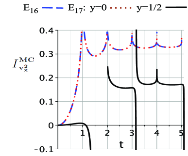
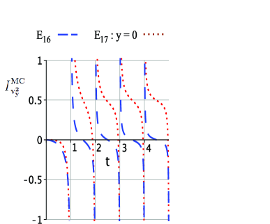
Figure 1 also shows that for the particle’s position in the orientability indicator curves coincide with those for a generic point in globally homogenous . This shows that for , where the global inhomogeneity degree of freedom is frozen, the -component of the orientability indicator cannot be used to distinguish between the two orientable and non-orientable spaces. With different pattern of curves, the same holds true for the -components of the orientability indicator for and , but we do not show this figure for the sake of brevity. This result on these two components of the orientability indicator can be read from our equations. Indeed, for the particle’s position at for , taking account of (22) – (25) it is straightforward to show that Eqs. (19) and (21) reduce, respectively, to (26) and (27). However, it should be noticed that even for the -component of the orientability indicator does not reduce to . This means that in order to extract information regarding orientability from the motion of a charged particle under electromagnetic fluctuations the proper comparison should be between the -components of the dispersion, as we do in Fig. 2. This was to be expected from the outset since the reflection holonomy for is in the -direction (cf. Table 2).
Figure 2 displays the -components of the orientability indicator for a charged test particle in Minkowski space whose spatial section has (orientable) and [non-orientable, ] topologies. The chief conclusion is that the component along the direction of the flip (cf. Table 2) might be used to find out whether the particle lies in Minkowski spacetime with orientable or non-orientable space. Figure 2 also shows different orientability indicator curves for and which, in both cases, repeat themselves periodically. For the two topologies the overall patterns of the orientability indicator curves are similar.
Although the above result seems valuable to the extent that it makes clear the strength of our approach to access orientability through electromagnetic vacuum fluctuations, it demands a comparison between the orientability indicator curves for the two given spatial manifolds for a verdict about orientability. Thus, it does not provide a conclusive answer to the central question of this paper, namely how to locally probe the orientability of the spatial section of Minkowski spacetime in itself from electromagnetic vacuum fluctuations. Given the directional properties of a point electric dipole, a pertinent question that emerges here is whether it would be more effective to use it for testing the individual non-orientability of a generic space. If so we could envisage a local experiment to probe the orientability of a space per se. In the next subsection we shall investigate this remarkable possibility.
3.2 NON-ORIENTABILITY WITH POINT ELECTRIC DIPOLE
A noteworthy outcome of the previous section is that the time evolution of the velocity dispersion for a charged particle can be used to locally differentiate an orientable () from a non-orientable () spatial section of Minkowski spacetime. However, it cannot be used to decide whether a given space manifold is or not orientable. In this way, it cannot be taken as a definite answer to our central question about the spatial orientability of Minkowski spacetime. So, a question that naturally arises here is whether the velocity dispersion of a different type of point-like particle could provide a suitable local signature of non-orientability. As a point electric dipole has directional properties, one might expect that its orientability indicator would potentially be more effective in providing information regarding non-orientability associated with a particular direction. To examine this issue we now turn our attention to topologically induced motions of an electric dipole under quantum vacuum electromagnetic fluctuations.
Newton’s second law for a point electric dipole of mass in an external electric field reads
| (28) |
where is the electric dipole moment. With the same hypotheses as for the point charge and assuming the dipole is initially at rest, integration of Eq. (28) yields
| (29) |
with and summation over repeated indices implied.
The mean squared speed in each of the three independent directions is given by
| (30) |
which can be conveniently rewritten as
| (31) |
where .
Now we proceed to the computation of the velocity dispersion for a point dipole in spaces and . The space has two topologically conspicuous directions: the compact -direction and the flip -direction associated with the non-orientability of . To probe the non-orientability of by means of stochastic motions, it seems most promising to choose a dipole oriented in the -direction, since the orientation of the dipole would also be flipped upon every displacement by the topological length along the compact direction. Indeed, it is for a dipole oriented in the flip direction that the effect of the non-orientability is most noticeable, as we show in the following.
For a dipole oriented along the axis the dipole moment is and we again use the indicator in which the electric field correlation functions are replaced by their renormalized counterparts, as in equation (15) for the charged point particle. We have
| (32) |
where the left superscript within parentheses indicates the dipole’s orientation. With the help of Eq. (11) the -component of the orientability indicator for the slab space with flip takes the form
| (33) |
with defined by Eq. (9) and , while is given by Eq. (3.1). Making use of
| (34) |
we find
| (35) |
where, with ,
| (36) |
| (37) |
| (38) |
Similar calculations lead to
| (39) | |||||
and
| (40) |
Since the coincidence limit has been taken, it follows from Eq. (3.1) that in Eqs. (3.2) to (3.2) one must put
| (41) |
It can be immediately checked that, as for the point charge, in the Minkowskian limit () the orientability indicator for a dipole is zero.
For the slab space the components of the dipole orientability indicator are obtained from those for by setting , and replacing by everywhere. Therefore, we have
| (42) | |||||
| (43) | |||||
| (44) |
in which .

NON-ORIENTABILITY WITH A DIPOLE – CONCLUSIONS
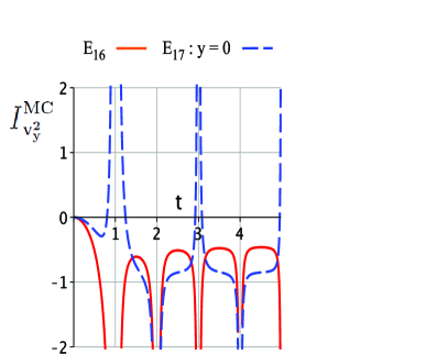
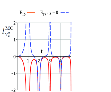
We begin by noting that the expressions (3.2)-(3.2) and (42)-(44) for the components of the orientability indicator for and topologies, respectively, are too involved to lend themselves to a straightforward interpretation. Nevertheless, something significant can be said: for a dipole located at all components of the orientability indicator for are different from those for because each summand in Eqs. (3.2), (39) and (3.2) contains the prefactor which is absent from the corresponding Eqs. (42) – (44) for . Since not much further can be read from our equations, in order to demonstrate our main result, which is ultimately stated in terms of patterns of curves for the orientability indicator, we begin by plotting figures for the components of the orientability indicator. Figures 3 to 5 come from Eqs. (3.2) – (3.2) as well as (42) – (44), with the topological length and ranging from to . In the three figures the solid lines stand for the orientability indicator curves for the dipole in Minkowski spacetime with orientable spatial topology, whereas the dashed lines represent orientability indicator curves for the dipole located at in a space with non-orientable topology.
In the case of the -component, the time evolution curves of the orientability indicator for and , shown in Fig. 3, present a common periodicity but with clearly distinguishable patterns. The orientability indicator curve for displays a distinctive sort of periodicity characterized by an inversion pattern. Non-orientability gives rise to this pattern of consecutive inversions, which is not present for the orientable .
The differences become more salient when one considers the other two components of the orientability indicator, shown in Figs. 4 and 5. For both of these components, the non-orientability of is disclosed by an inversion pattern whose structure is more striking than the one for the -component. The orientability indicator curves for form a pattern of alternating upward and downward “horns”, making the non-orientability of unmistakably identifiable.
From the above analysis of Figs. 3 to 5 as compared with the corresponding analysis of Fig. 2, we see that the point dipole is potentially a much more efficient non-orientability probe than the point particle. Furthermore, the characteristic inversion pattern exhibited by the dipole indicator curves makes it possible to identify the non-orientability of by itself, without having to make a comparison with the indicator curves for its orientable counterpart. We have checked, although we do not show the calculations, that for a dipole located at and oriented either in the -direction or in the -direction, only the -component of the orientability indicator for is different from the one for . Thus, it is for a dipole oriented in the flip direction that the non-orientability of is most sharply exposed.
This discussion suggests that it may be possible to unveil a presumed spatial non-orientability by local means, namely by the stochastic motions of point particles caused by quantum electromagnetic vacuum fluctuations. If the motion of a point electric dipole is taken as probe, non-orientability can be intrinsically discerned by the inversion pattern of the dipole’s orientability indicator curves.
To close this section, some additional words of clarification regarding the use of the orientability indicator are fitting. We first note that, from a theoretical viewpoint, similarly to the way we calculated the orientability indicator for and topologies [(3.2) – (3.2) and (42) – (44)] one can use the indicator’s definition (16) to derive analytic expressions and plot corresponding curves for all eight non-orientable Euclidean topologies for a dipole. This set of theoretical curves for the orientability indicator would form a collection of curve patterns that are signatures of non-orientability, and which can be compared with experimental curves to find out about orientability of space. From the experimental standpoint there are two main approaches to the use of . One is to contrast theory and observation through engineered experiments. This would be useful to check the different expressions we have derived for against experimental data. In this case, one would need to manufacture devices that simulate non-trivial topologies. However, experimental apparatuses to mimic non-trivial topologies are not easy to prepare.111111For a very simple nontrivial topology such as the space reflection orbifold a perfectly reflecting plane should simulate the topology. Along these lines, one might wonder whether many equally spaced perfectly reflecting planes would simulate . Simulation of nontrivial topologies in laboratory is indeed a thorny issue for experimentalists, for it depends on the physical phenomena involved. This issue is beyond the scope of the present work, but we mention that in a different context examples of simulations of non-trivial topologies such as the cylinder, the torus and the non-orientable Möbius strip have been recently discussed Boada-etal-2015 .
Another experimental approach is to use the indicator to directly access orientability of the spatial section of Minkowski spacetime. First one would measure the velocity correlation functions for . Then one would subtract out the theoretically-computed correlation functions for topologically trivial (simply-connected) Minkowski spacetime, which are given in the Appendix. The corresponding curves for this difference would be plotted in the coincidence limit and contrasted with each of the eight theoretical curves mentioned in the previous paragraph.
4 Conclusions and final remarks
In general relativity and quantum field theory spacetime is modeled as a differentiable manifold, which is a topological space equipped with an additional differential structure. Orientability is an important topological property of spacetime manifolds. It is often assumed that the spacetime manifold is orientable and, additionally, that it is separately time and space orientable. The theoretical arguments usually offered to assume orientability combine the space-and-time universality of local physical experiments121212The space universality can be looked upon as a topological assumption of global spatial homogeneity, which in turn rules out spatial non-orientability of space. with physically well-defined (thermodynamically, for example) local arrow of time, violation of charge conjugation and parity (CP violation) and CPT invariance Zeldovich1967 ; Hawking ; Geroch-Horowitz-1979 . Another theoretical argument in favor of a time- and space-orientable spacetime comes from the impossibility of having globally defined spinor fields on non-orientable spacetime manifolds. One can certainly use such reasonings in support of the standard assumptions on the global structure of spacetime. 131313See Ref. MarkHadley-2018 for a dissenting point of view, and also the related Ref. MarkHadley-2002 . Nevertheless, it is reasonable to expect that the ultimate answer to questions regarding the orientability of spacetime should rely on cosmological observations or local experiments, or might come from a fundamental theory of physics.
In the physics at daily and even astrophysical length and time scales, we do not find any sign or hint of non-orientability. This being true, the remaining open question is whether the physically well-defined local orientations can be extended continuously to cosmological scales.
At the cosmological scale, one would think at first sight that to disclose spatial orientability one would have to make a trip around the whole space to check for orientation-reversing paths. Since such a global journey across the Universe is not feasible one might think that spatial orientability cannot be probed globally. However, a determination of the spatial topology through the so-called circles in the sky CSS1998 , for example, would bring out as a bonus an answer to the space orientability problem at the cosmological scale.141414 In the searches for these circles so far undertaken, including the ones carried out by the Planck Collaboration Planck-2013-XXVI ; Planck-2015-XVIII , no statistically significant pairs of matching circles have been found (see Ref. Vaudrevange-etal-12 for the most extensive search yet, and also references therein for the other searches). These negative observational results, however, are not sufficient to exclude the possibility that the Universe has a detectable (orientable or non-orientable) nontrivial topology (see Ref. Gomero-Mota-Reboucas-2016 for some limits of these searches).
There is no reason in the classical physics of point-like particles to force a spacetime manifold to be orientable. However, the situation changes once fermions, for example, are considered at the quantum level. Indeed, in quantum field theory one uses spinors to describe fermions. This fact inevitably leads to the inclusion of spinors as desirable objects (locally) in the spacetime on physical grounds. However, the global question, which ultimately is not a physical requirement, is left open and the assumption of existence of globally defined spinor fields, which rules out non-orientable spacetimes Penrose-1968 ; Penrose-Hindler1986 ; Geroch-1968 ; Geroch-1970 , comes from theoretical arguments that combine this local physics requisite with the space-and-time universality of the basic local rules of physics. For spacetimes of the form , the spatial universality (see related comment on p.288 of Visser Visser-1996 ), can be mathematically translated in terms of global (topological) homogeneity of , which in turn rules out spatial non-orientability of the space since there is no globally homogeneous non-orientable quotient manifold . As a matter of fact, the spatial universality alone as captured in topological terms rules out not only the non-orientable but any topologically inhomogeneous spatial sections . In this way, in arguing for the universality of the local physics, which would lead to the existence of globally defined spinor fields, we are actually making a topological assumption of global homogeneity of space, which itself excludes the non-orientable manifolds and also the remaining other globally inhomogeneous and orientable spatial sections.151515In technical terms, the ultimate mathematical point that leads to the fact that we cannot have globally defined spinor fields in non-orientable manifolds lies in bringing together the two-valuedness of spinors with the flip holonomy. Actually, this mismatching occurs even in some orientable, but inhomogeneous, quotient manifolds , whose covering or holonomy group contains at least one which is a proper screw motion with (cf. Section II). In brief, one can only have global spinor fields in spacetimes whose spatial section is globally (topologically) homogeneous. This obviously excludes the topologically inhomogeneous , whose set contains all non-orientable space manifolds.
In this paper we have addressed the question as to whether electromagnetic quantum vacuum fluctuations can be used to bring out the spatial orientability of Minkowski spacetime. To this end, we have studied the stochastic motions of point-like particles under quantum electromagnetic fluctuations in Minkowski spacetime with the orientable slab space () and the non-orientable slab space with flip () topologies (cf. Tables 1 and 2).
For a point charged particle, we have derived analytic expressions for the orientability indicator, namely Eqs. (19) – (25) for space topology, and Eqs. (26) – (27) for space topology. From these equations we have made Fig. 1 and Fig. 2. Using these equations and figures we have shown that it is possible to distinguish the orientable from the non-orientable topology by contrasting the time evolution of the respective orientability indicators along the flip direction of .
In spite of being a significant result in that it makes apparent the power of our approach to access orientability through electromagnetic quantum vacuum fluctuations, it is desirable, however, to be able to decide about the orientability of a given spatial manifold in itself. To tackle this question, motivated by a dipole’s directional properties, we have then examined whether the study of stochastic motions of a point-like electric dipole would be more effective for testing the non-orientability of a generic space individually, i.e. without having to make a comparison of the results for an orientable space with those for its non-orientable counterpart.
To this end, we have derived the expressions for the orientability indicators given by equations (3.2) – (3.2) for the dipole oriented in the flip direction in the non-orientable space with topology, and equations (42) – (44) for the dipole in the orientable space with topology. From these equations we have calculated and plotted Figures 3 to 5. As a result of the analysis of these equations and figures we have found that there exists a characteristic inversion pattern exhibited by the orientability indicator curves in the case of , signaling that the non-orientability of might be identified per se. The inversion pattern of the orientability indicator curves for the dipole is a signature of the reflection holonomy, and ought to be present in the orientability indicator curves for the dipole in all remaining seven non-orientable topologies with flip, namely the four Klein spaces ( to ) and those in the chimney-with-flip class ( to ).161616See Refs. Riazuelo-et-el03 ; Fujii-Yoshii-2011 for the symbols, names and properties of Klein spaces and chimney-with-flip families of non-orientable topologies. Clearly the inversion patterns for the electric dipole change with the associated topology: different topologies give rise to curves for the orientability indicator with distinct inversion patterns.
A short comment on how our results extend to the quantum level is fitting. We have tacitly assumed that the charged object of interest is described by a well-localized wave packet. Our classical analysis is justified because it has been argued [16] that under suitable conditions the dispersion due to wave packet spreading is negligible as compared with the dispersion brought about by vacuum fluctuations of the electromagnetic field.
Observation of physical phenomena and experiments are fundamental to our understanding of the physical world. Our results indicate that it is potentially possible to locally unveil spatial non-orientability through stochastic motions of point-like particles under electromagnetic quantum vacuum fluctuations. In this way, the present paper may be looked upon as an intimation of a conceivable way to locally probe the spatial orientability of Minkowski empty spacetime. A different statistical indicator of the stochastic motions can certainly be conceived, but perhaps the most important point raised in this work is that the spatial orientability of spacetime can be locally probed by inquiring quantum vacuum electromagnetic fluctuations about the motion of point-like “charged” particles.
Acknowledgements.
M.J. Rebouças acknowledges the support of FAPERJ under a CNE E-26/202.864/2017 grant, and thanks CNPq for the grant under which this work was carried out. We also thank C.H.G. Bessa for fruitful discussions and for his help with the figures. M.J.R. is also grateful to A.F.F. Teixeira for interesting comments, and also for reading the manuscript and indicating typos.Appendix A Velocity correlation functions for the simply-connected space
In this appendix we give the velocity correlations functions for simply-connected spatial section of Minkowski spacetime that are referred to on the last paragraph of Section 3, for both the point particle and the point dipole. These are calculated as follows. First replace in equation (5) by as given by (6), thus obtaining the electric field correlation functions for the topologically trivial (simply connected) Minkowski spacetime. Then insert these electric field correlation functions with into the right-hand side of equation (4), for the particle, and equation (30), for the dipole. With
| (45) |
and
| (46) |
we have, for the particle:
| (47) | |||||
| (48) | |||||
| (49) | |||||
The corresponding results for the dipole oriented in the -direction are
| (50) | |||||
| (51) | |||||
| (52) | |||||
where the integrals , , are given by equations (3.2) to (3.2).
References
- (1) G.F.R. Ellis, Gen. Rel. Grav. 2, 7 (1971); M. Lachièze-Rey and J.P. Luminet, Phys. Rep. 254, 135 (1995); G.D. Starkman, Class. Quantum Grav. 15, 2529 (1998); J. Levin, Phys. Rep. 365, 251 (2002); M.J. Rebouças and G.I. Gomero, Braz. J. Phys. 34, 1358 (2004); M.J. Rebouças, A Brief Introduction to Cosmic Topology, in Proc. XIth Brazilian School of Cosmology and Gravitation, eds. M. Novello and S.E. Perez Bergliaffa (Americal Institute of Physics, Melville, NY, 2005) AIP Conference Proceedings vol. 782, p 188, also: arXiv:astro-ph/0504365; J.P. Luminet, Universe 2016, 2(1), 1.
- (2) M.J. Rebouças, Detecting cosmic topology with primordial gravitational waves, in preparation (2021).
- (3) G.I. Gomero, M.J. Rebouças, and R. Tavakol, Class. Quantum Grav. 18, 4461 (2001); G.I. Gomero, M.J. Rebouças, and Reza K. Tavakol, Class. Quant. Grav. 18, L145 (2001); G.I. Gomero, M.J. Rebouças, and R. Tavakol, Class. Quantum Grav. 18, L145 (2001); G.I. Gomero, M.J. Rebouças, and R. Tavakol, Int. J. Mod. Phys. A 17, 4261 (2002); J. Weeks, Mod. Phys. Lett. A 18, 2099 (2003); B. Mota, M.J. Rebouças, and R. Tavakol, Class. Quantum Grav. 20, 4837 (2003).
- (4) P.M. Vaudrevange, G.D. Starkman, N.J. Cornish, and D.N. Spergel, Phys. Rev. D 86, 083526 (2012).
- (5) P.A.R. Ade, et al. (Planck Collaboration 2013), Astron. Astrophys. 571, A26 (2014).
- (6) P.A.R. Ade et al. (Planck Collaboration 2015), Astron. Astrophys. 594, A18 (2016).
- (7) G. Gomero, B. Mota, and M.J. Rebouças, Phys. Rev. D 94, 043501 (2016).
- (8) J.A. Wolf, Spaces of Constant Curvature (McGraw-Hill, New York, 1967).
- (9) W.P. Thurston, Three-Dimensional Geometry and Topology. Vol.1, Edited by Silvio Levy (Princeton University Press, Princeton, 1997).
- (10) B.S. DeWitt, C.F. Hart and C.J. Isham, Physica 96A, 197 (1979).
- (11) J.S. Dowker and R. Critchley, J. Phys. A 9, 535 (1976).
- (12) P.M. Sutter and T. Tanaka, Phys. Rev. D 74, 024023 (2006).
- (13) M.P. Lima and D. Muller, Class. Quant. Grav. 24, 897 (2007).
- (14) D. Muller, H.V. Fagundes, and R. Opher, Phys. Rev. D 66, 083507 (2002).
- (15) D. Muller, H.V. Fagundes, and R. Opher, Phys. Rev. D 63, 123508 (2001).
- (16) H. Yu and L.H. Ford, Phys. Rev. D 70, 065009 (2004).
- (17) H. Yu and J. Chen, Phys. Rev. D70, 125006 (2004).
- (18) L.H. Ford, Int. J. Theor. Phys. 44, 1753 (2005).
- (19) H.W. Yu, J. Chen, and P. X. Wu, JHEP 0602, 058 (2006).
- (20) C.H.G. Bessa, V.B. Bezerra, and L.H. Ford, J. Math. Phys. 50, 062501 (2009).
- (21) V. Parkinson and L.H. Ford, Phys. Rev. A 84, 06210 (2011).
- (22) V.A. De Lorenci, C.C.H. Ribeiro, and M. M. Silva, Phys. Rev. D 94, 105017 (2016).
- (23) M. Seriu and C.H. Wu, Phys. Rev. A 77, 022107 (2008).
- (24) G. Gour and L. Sriramkumar, Found. Phys. 29, 1917 (1999).
- (25) M. T. Jaekel and S. Reynaud, Quant. Opt. 4, 39 (1992).
- (26) C.H.G. Bessa and M.J. Rebouças, Class. Quantum Grav. 37, 125006 (2020).
- (27) E. Feodoroff, Russ. J. Crystallogr. Mineral. 21, 1 (1885).
- (28) L. Bieberbach, Math. Ann. 70, 297 (1911).
- (29) L. Bieberbach, Math. Ann. 72, 400 (1912).
- (30) W. Novacki, Comment. Math. Helv. 7, 81 (1934).
- (31) C. Adams and J. Shapiro, American Scientist 89, 443 (2001).
- (32) B. Cipra, What’s Happening in the Mathematical Sciences (American Mathematical Society, Providence, RI, 2002).
- (33) A. Riazuelo, J. Weeks, J.P. Uzan, R. Lehoucq, and J.P. Luminet, Phys. Rev. D 69, 103518 (2004).
- (34) H. Fujii and Y. Yoshii, Astron. Astrophys. 529, A121 (2011).
- (35) J. Anandan, Phys. Rev. Lett. 81, 1363 (1998).
- (36) J.R. Weeks, The Shape of Space, 3rd ed. (CRC Press, Boca Raton, FL, 2020).
- (37) N.D. Birrel and P.C.W. Davies, Quantum Fields in Curved Space (Cambridge University Press, Cambridge, 1982).
- (38) J. Chen and H.W. Yu, Chin. Phys. Lett. 37, 2362 (2004).
- (39) R. Lehoucq, M. Lachièze-Rey & J.-P. Luminet, Astron. Astrophys. 313, 339 (1996).
- (40) G.I. Gomero, M.J. Rebouças, and A.F.F. Teixeira, Class. Quantum Grav. 18, 1885 (2001).
- (41) G.I. Gomero, A.F.F. Teixeira, M.J. Rebouças, and A. Bernui, Int. J. Mod. Phys. D 11, 869 (2002).
- (42) M.J. Rebouças Int. J. Mod. Phys. D 9 561 (2000).
- (43) L.S Brown and G.J. Maclay, Phys. Rev. 184, 1272 (1969).
- (44) V.A. De Lorenci, and C.C.H. Ribeiro, JHEP 1904, 072 (2019).
- (45) O. Boada, A. Celi, J. Rodríguez-Laguna, J. Latorre, M. Lewenstein, New J. Phys. 17, 045007 (2015).
- (46) Ya.B. Zeldovich and I.D. Novikov, JETP Letters 6, 236 (1967).
- (47) S.W. Hawking and G.F.R. Ellis, The Large Scale Structure of Space-Time (Cambridge University Press, Cambridge, 1973).
- (48) R. Geroch and G.T. Horowitz, Global structure of spacetimes in General relativity: An Einstein centenary survey, pp. 212-293, Eds. S. Hawking and W. Israel (Cambridge University Press, Cambridge, 1979).
- (49) M. Hadley, Testing the Orientability of Time. Preprints 2018, 2018040240.
- (50) M. Hadley, Class. Quantum Grav. 19, 4565 (2002).
- (51) N.J. Cornish, D. Spergel, and G. Starkman, Class. Quantum Grav. 15, 2657 (1998).
- (52) R. Penrose, The Structure of Space-Time, in BattelIe Rencontres in Mathematics and Physics: Seattle, 1967, C. M. DeWitt and J. A. Wheeler, Eds. (Benjamin, New York, 1968).
- (53) R. Penrose and W. Rindler, Spinors and Space-time, Volume 1, Two-spinor calculus and relativistic fields (Cambridge University Press, Cambridge, 1986).
- (54) R. Geroch, J. Math. Phys. 9, 1739 (1968).
- (55) R. Geroch, J. Math. Phys. 9, 343 (1970).
- (56) M. Visser, Lorentzian Wormholes from Einstein to Hawking (AIP, New York, 1996).