GPA: A GPU Performance Advisor Based on Instruction Sampling

Abstract.

Developing efficient GPU kernels can be difficult because of the complexity of GPU architectures and programming models. Existing performance tools only provide coarse-grained suggestions at the kernel level, if any. In this paper, we describe GPA, a performance advisor for NVIDIA GPUs that suggests potential code optimization opportunities at a hierarchy of levels, including individual lines, loops, and functions. To relieve users of the burden of interpreting performance counters and analyzing bottlenecks, GPA uses data flow analysis to approximately attribute measured instruction stalls to their root causes and uses information about a program’s structure and the GPU to match inefficiency patterns with suggestions for optimization. To quantify each suggestion’s potential benefits, we developed PC sampling-based performance models to estimate its speedup. Our experiments with benchmarks and applications show that GPA provides an insightful report to guide performance optimization. Using GPA, we obtained speedups on a Volta V100 GPU ranging from 1.01$\times$ to 3.53$\times$, with a geometric mean of 1.22$\times$.

1. Introduction

Graphics Processing Units (GPUs) have been extensively employed in data centers and supercomputers as a building block to accelerate High-Performance Computing (HPC) and machine learning applications. However, fully utilizing the compute power of GPUs is challenging. Tuning GPU code to achieve the maximum possible performance requires significant manual effort to cope with the complexity of GPU architectural features and programming models.

GPU profilers (nvp, 2019; NVIDIA Corporation, 2020c, b; Zhou et al., 2020; Shende and Malony, 2006; Mey et al., 2012; January et al., 2015) are widely used for measuring GPU-accelerated applications. While these tools identify hot GPU code, they lack sophisticated analysis of performance bottlenecks and provide little insight into how to improve the code. nvprof and Nsight-Compute, for example, analyze performance measurement data and propose suggestions on the kernel level but do not identify specific lines that could be optimized nor estimate the potential gain after applying optimizations. As a result, even with GPU profilers, diagnosing and fixing performance problems requires expertise in interpreting measurement data and associating suggestions with corresponding bottlenecks.

Prior tools on GPUs (Shen et al., 2018; gvp, 2020; Braun and Fröning, 2019) provide fine-grained suggestions using instrumentation-based methods to quantify the severity of performance problems and locate problematic code. These tools identify one or a few patterns, such as redundant value/address, insufficient cache utilization, or memory transaction burst, but overlook others. Moreover, they do not correlate execution time with the patterns. As a result, one may fix specific problems indicated by the tools but not achieve any speedup.

Modern processors support fine-grain measurement using sampling (Dean et al., 1997; Drongowski, 2007; Guide, 2011; Corporation, 2019), which can be used to study instruction statistics in applications quantitively. Unique among GPU vendors, NVIDIA implements PC sampling on its GPUs to sample instructions and associate them with stall reasons. Existing performance tools (Shende and Malony, 2006; Zhou et al., 2020; Zhang and Hollingsworth, 2019; NVIDIA Corporation, 2020b; January et al., 2015) that utilize PC sampling only associate instruction samples with source lines of GPU code where the stalls occur but lack the ability to derive performance insight based on stall reasons.

To complement the aforementioned approaches, we propose GPA—a GPU performance advisor that suggests effective optimizations for GPU code, and evaluate GPA on a V100 GPU with the Rodinia benchmarks (Che et al., 2009), several larger application benchmarks, and a combustion application. Guided by GPA, we improved the performance of the GPU kernels studied by 1.03x to 3.86x. This paper describes the design and implementation of GPA which consists of the following key components:

• An instruction blamer that attributes stalls to instructions that cause them;

• Performance optimizers that match inefficiency patterns with optimization suggestions for lines, loops, and functions based on program structure, architectural features, measurement data, and control flow;

• Performance estimators that model GPU execution using instruction samples to estimate speedups for each optimizer.

This rest of the paper is organized as follows. Section 2 reviews PC sampling and instruction format on NVIDIA’s GPUs. Section 3 introduces the workflow of GPA. Section 4 explains the details of GPA’s instruction blamer. Section 5 describes the implementation of GPA’s preformance optimizers and estimators. Section 6 describes the analysis and optimization of GPU kernels using GPA. Section 7 presents case studies of four larger codes, including a combustion application. Section 8 reviews related work and distinguishes GPA. Finally, Section 9 summarizes our work and outlines our plans for future work.

2. Background and Motivation

Table 1. Dissection of the fields of “@P0 LDG.32 R0, [R2]” instruction.

Wait Mask	Write Barrier	Read Barrier	Predicate	Opcode	Modifiers	Destination Operands	Source Operands
B0	B1		P0	LDG	32	R0	R2, R3

In this section, we describe background necessary to understand our work and our motivation for developing GPA. In Section 2.1, we introduce a model of the PC sampling mechanism implemented in recent NVIDIA GPUs. In Section 2.2, we describe the instruction format used by NVIDIA’s GPUs, which is important for instruction dependency analysis. In Section 2.3, we show how raw PC sampling measurements are insufficient to provide insight for performance optimization.

2.1. PC Sampling

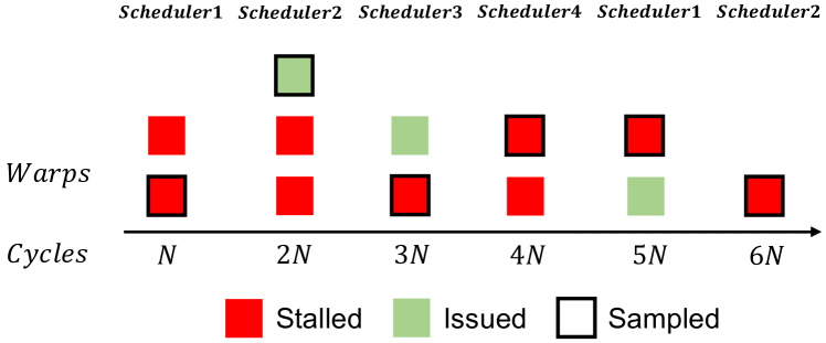
Figure 1. A mental model of PC sampling on an SM of NVIDIA’s V100 GPU. Samples are taken every $N$ cycles. Samples at $N$, 4$N$, and 6$N$ are latency samples, and others are active samples. Samples at $N$, 3$N$, 4$N$, 5$N$, and 6$N$ are stall samples.

NVIDIA’s GPUs implement PC sampling to collect instruction samples. One can use NVIDIA’s CUPTI API (NVIDIA Corporation, 2019) to collect PC samples for GPU-accelerated applications. Each streaming multi-processor (SM) in an NVIDIA GPU collects samples individually. When a buffer used to collect samples is full on an SM, CUPTI merges samples from all SMs and transfers the samples to the CPU.

Each SM on an NVIDIA V100 has four warp schedulers, and each warp scheduler is assigned a number of active warps. At the end of each sampling period, an SM records a sample for one of its warp schedulers and it cycles through its warp schedulers in a round-robin fashion. When a warp is sampled, two classes of samples are recorded: an active sample when the warp scheduler is issuing an instruction and a latency sample when no instruction is issuing. For the instruction sampled, a stall reason (e.g., waiting for a value from memory) is recorded for the instruction, if any. Consider Figure 1 as an example. There are 5 samples with a stall reason. We call them stall samples or stalls in the remaining sections. Because there are three latency samples and three active samples, we estimate the stall ratio and the active ratio of the SM as $3/6$. Assuming all SMs on the GPU have a similar workload, we estimate the stall ratio and the active ratio of the GPU kernel as $3/6$.

2.2. Instruction Format

A fixed length instruction encoding is used on NVIDIA’s GPUs. Pre-Volta GPUs use a 64-bit word for an instruction, but Volta and later architectures use a 128-bit word. In this paper, we focus on the Volta architecture used in two of the top three supercomputers—Summit and Sierra.

Among the fields of a GPU instruction shown in Table 1, we focus on the following three key fields:

• Wait Mask and Write/Read Barrier. Every GPU instruction has a control code (Jia et al., 2018; Zhang et al., 2017) field that encodes information to guide the warp scheduler as it issues instructions, including stall cycles, yielding flag, and dependencies. For each fixed latency instruction (e.g., most arithmetic instructions), the assembler sets stall cycles for the instruction to indicate how long the scheduler should wait before issuing the instruction. For each variable latency instruction, the assembler associates write/read barrier indices with it, and associates instructions that depend on them a wait mask to create dependencies.

• Predicate. If an instruction’s predicate field is set, the instruction is executed when the predicate evaluates as true. There are both true and false predicate conditions: Pi is a true predicate condition, and !Pi is a false predicate condition, where $0\leq i\leq 6$. In Table 1, the LDG instruction is executed if P0 is true.

• Opcode, Modifiers, and Operands. Each thread can use up to 255 32-bit regular registers ranging from R0-R254. Opcode and modifiers together determine the length of operands used. In Table 1, the 32 modifier indicates each thread reads a 32-bit value from memory. Moreover, because the data is loaded from global memory, which has a 64-bit address space, the source operand is a 64-bit value comprised of two registers—R2 and R3.

2.3. Motivating Examples

We refer to a collection of instruction samples and their stall reasons as a raw PC sampling report from which we can measure the stall reasons of a kernel. However, diagnosing the slowness of the kernel still requires interpretation of the measurement data to answer the following questions.

• Which GPU instructions cause stalls?

• How can we improve the performance by eliminating these stalls?

• What is the estimated speedup for each potential optimization?

To illustrate the importance of analyzing stall reasons and associating them with optimizations, we analyze the hotspot and the b+tree examples in Rodinia benchmark.

⬇

1for (int i = 0; i < iteration; i++) {

2 temp_t[ty][tx] =

3 temp_on_cuda[ty][tx] + step_div_Cap * (

4 power_on_cuda[ty][tx] + (temp_on_cuda[S][tx] +

5 temp_on_cuda[N][tx] - 2.0 * temp_on_cuda[ty][tx]) *

6 ...

7}

Listing 1: A hot loop in the hotspot example

Listing 1 shows a hot loop of the hotspot kernel. The raw PC sampling report for this kernel indicates large execution latency stalls on Line 2, but it provides little information regarding where the stalls come from and what optimizations apply. GPA attributes the latency to type conversion instructions that demote a 64-bit float to a 32-bit float. Though all arrays are composed of 32-bit values, the compiler generates conversion instructions as a float constant multiplies a 32-bit float value. GPA suggests specifying the type of the constant ($2.0$) as a 32-bit value to avoid conversion. After applying the optimization, we achieved a 1.14$\times$ speedup.

⬇

1for (int i = 0; i < height; i++) {

2 if ((knodesD[currKnodeD[bid]].keys[thid] <= startD[bid]) &&

3 (knodesD[currKnodeD[bid]].keys[thid+1] > startD[bid]))

4 ...

5 __syncthreads();

6}

Listing 2: A hot loop in the b+tree example

Listing 2 shows a costly loop in the b+tree code. The raw PC sampling report shows high memory dependency stalls on Line 2 but does not propose a suggestion to eliminate the bottleneck. By analyzing the assembly code, GPA concludes that the distance between the load instructions and the instruction that consumes the loaded values is short. Therefore, instructions in the path are not enough to hide the latency. GPA suggests the users separate the subscripted loads from their uses by reordering code. We read the address of knodesD[currKnodeD[bid]].keys for the next iteration before the synchronization on Line 5 and obtained a 1.16$\times$ speedup.

Based on the analysis above, we conclude that pure PC sampling information is insufficient to guide optimizations. To improve the quality of the analysis report, we analyze instruction dependencies to characterize stalls’ causes. Furthermore, we can associate the stalls with the program’s structure to suggest code optimizations, such as loop unrolling, function inlining, and code reordering.

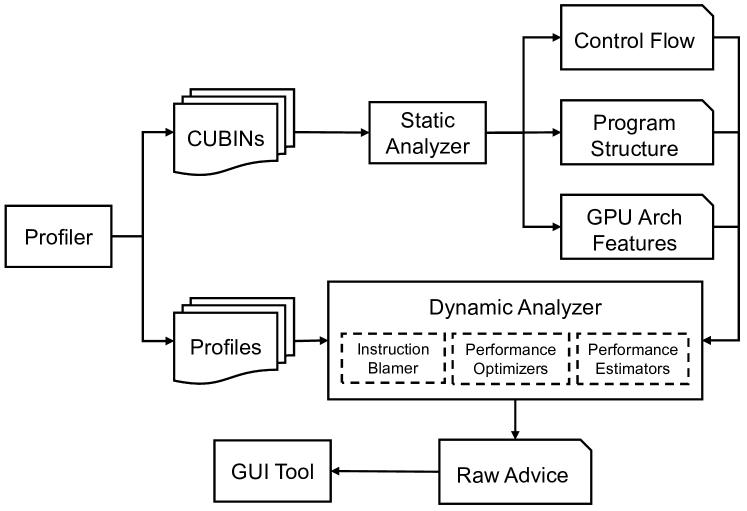
Figure 2. Overview of GPA

3. Overview

Figure 2 shows the workflow of GPA. GPA uses a profiler to collect PC samples and kernel launch statistics at runtime and attribute them to the calling context where the kernel is launched. The profiler dumps the profiles and records CUDA binaries (CUBINs) for offline analysis. GPA’s static analyzer analyzes CUBINs to recover static information which is ingested into the dynamic analyzer with profiles to generate comprehensive raw advice.

Static Analyzer

In its static analyzer, GPA analyzes CUBINs to recover the following files:

• Control flow graphs. GPA employs NVIDIA’s nvdisasm tool to decode instructions in CUBINs and dump raw control flow graphs. We modify the raw control flow graphs by splitting super blocks into basic blocks and ingest the modified control flow graphs into Dyninst (of Wisconsin-Madison, [n.d.]) to analyze loop nests.

• Program structure. A program structure file contains functions symbols, inline stacks, loop nests, and source line mappings. According to each function symbol’s visibility field, we annotate global functions and device functions. We read DWARF information to parse information about inlined functions.

• Architectural features. Based on the architecture flag encoded in CUBINs, we fetch specific hardware configurations, such as instruction latencies, warp size, and register limitations for analysis in the later stages.

Dynamic Analyzer

The dynamic analyzer is comprised of three components, including an instruction blamer, performance optimizers, and performance estimators.

We analyze each GPU kernel’s launch context separately. For each kernel invocation, the instruction blamer uses backward slicing (Cifuentes and Fraboulet, 1997; Srinivasan and Reps, 2016) to attribute stalls to the responsible instructions. Based on the stall counts and GPA’s static analysis results, each performance optimizer attempts to match its optimization strategy to program regions that have high stall samples. Guided by performance models, performance estimators estimate each optimizer’s speedup based on the matched samples. Finally, GPA generates an advice report that contains suggestions from its top optimizers sorted by their estimated speedups.

In this paper, we focus on the implementation of GPA’s dynamic analyzer, which tackles the following unique challenges: (1) It extends the backward slicing algorithm for special fields (e.g., barriers) of a GPU instruction to track dependencies among GPU instructions. (2) It attributes stalls to their sources accurately because it incorporates pruning rules to cut down dependency sources. (3) Without code annotation, it derives a general performance model to quantify the benefits of each GPU optimizer.

Utilization of GPA

GPA is a command line tool that automates profiling and analysis stages. Since GPA uses sampling-based profiles, users do not need to change their program source code. To provide advice at the source line level, the only change required is adding compiler options to ensure that the compiler includes line mapping information in GPU binaries it generates. Users apply optimizations according to the raw advice generated by GPA. Today, GPA produces raw advice as ASCII text; however, its advice could be incorporated into a graphical user interface tool to analyze inefficient code regions and optimization suggestions.

4. Instruction Blamer

CUPTI associates stall reasons (Corporation, 2019) with instruction samples. Among the stall reasons, memory dependency, synchronization, and execution dependency stalls are caused by the source instructions rather than the instructions that suffer from stalls. Other stall reasons, such as memory throttling, are caused by instruction samples with the stall. To further characterize program bottlenecks with memory dependency, synchronization, and execution dependency stalls, we developed an instruction blamer that attributes stalls to the source instructions.

We first use backward slicing to analyze every instruction’s def-use chain in the control flow graph. According to the def-use chain and measurement data, we build an instruction dependency graph where each node is an instruction, annotated with its stalls, and each edge represents a def-use relation. Since not all edges cause stalls, we prune edges according to several heuristic rules. In the end, we apportion the stalls to its incoming edges based on the number of issued instructions and the length of each edge.

Backward slicing

We target intra function backward slicing (Cifuentes and Fraboulet, 1997) for GPU instructions because instructions in the same function cause most stalls. We find a stalled instruction’s immediate dependency sources because transitive dependencies are unlikely to cause the stalls. According to Table 1, several fields of a GPU instruction impact instruction dependencies, including operands, barriers, and predicate. We can begin with a traditional backward slicing algorithm for CPU instructions to analyze GPU operands, but barriers and predicates need special processing.

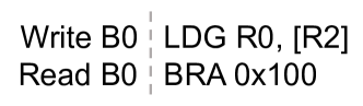
Figure 3. An example of barrier register dependency

Virtual barrier registers: We define six available barrier indices as six virtual barrier registers B0-B5. A write/read barrier index association can be represented as a write operation to one or more barrier registers. Likewise, we treat a wait mask association as a read of barrier registers. In this way, dependencies caused by barrier indices can be identified through def-use chains of the virtual barrier registers. It is worth noting that barriers can be set even if there is no dependency between regular registers. Take Figure 3 as an example, the LDG instruction loads a value to R0 and writes barrier B0, and the BRA instruction does not consume R0 but still reads B0. Observed memory dependency stalls on the BRA instruction should be attributed to the LDG instruction.

Predicated instructions: Immediate dependency sources are not only the first def instruction of each of its operands on the search path. Consider Figure 4(a) as an example, suppose we observe a stall at the IADD instruction, which does not have a predicate; because the LDG instruction is executed only if P0 is true, it is possible that the stall comes from the LDC instruction earlier in the path, which is executed only if P0 is false. Therefore, the backward slicing search should proceed until the predicates of def instructions on the path cover all conditions.

Let $P$ be the union of def instructions’ predicates on the path. $P=\cup p$, where $p\in\{p_{i}\}\cup\{!p_{i}\}\cup\{\_\}$, and $\{p_{i}\}\cup\{!p_{i}\}=\{\_\}$, for $0\leq i\leq 6$. $\_$ is a special predicate that covers both true and false predicates. An instruction without a predicate has the same semantic as $\_$. We say $P$ contains $p^{\prime}$ iff $p^{\prime}\in P$ or $\_\in P$. The backward slicing search proceeds until the union of def instructions’ predicates on the search path ($P$) contains the predicate of the use instruction ($p^{\prime}$).

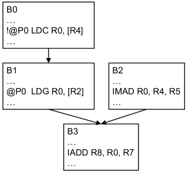
(a) Backward slicing

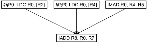
(b) Construct a dependency graph

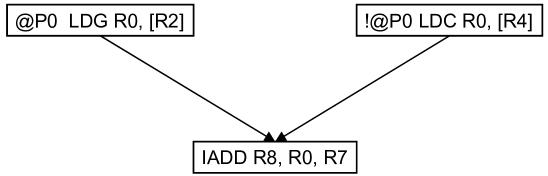
(c) Prune cold edges

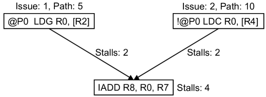
(d) Apportion stalls

Figure 4. Steps to attribute stalls of the IADD instruction

Construct a dependency graph

We build an instruction dependency graph from the def-use chains of collected instruction samples. For simplicity, in Figure 4(b) we only demonstrate memory dependency. Each node represents an instruction, and each edge represents a def-use relation associated with R0.

Prune cold edges

Not all the dependent edges cause stalls. If an edge does not trigger stalls, we call it a “cold edge” and use the following three rules to prune it.

1. Opcode based pruning. Memory dependency stalls are attributed to memory instructions only. Synchronization dependency stalls are attributed to synchronization instructions only.

2. Dominator based pruning. For every edge $e$ from node $i$ to $j$ in a dependency graph, we remove $e$ if there is a non-predicate instruction $k$ uses the same operands that $i$ defines and $j$ uses, and $k$ is in every path from $i$ to $j$ in the control flow graph because we would have observed stalls at $k$ rather than $j$ if $i$ caused any stalls.

3. Instruction latency based pruning. For every edge $e$ from node $i$ to $j$ in a dependency graph, we remove $e$ if the number of instructions in every path from $i$ to $j$ in the control flow graph is greater than the $latency$ of $i$.

For fixed latency instructions, we can use microbenchmarking (Jia et al., 2018) for their latencies; for variable latency instructions, we use their upper bounds for pruning. For instance, we use the TLB miss latency as the upper bound latency of global memory instructions.

According to the opcode pruning rule, we prune the edge from IMAD to IADD in Figure 4(b) to obtain the dependency graph in Figure 4(c) because an IMAD instruction cannot cause memory dependency stalls.

Attribute stalls

After pruning cold edges, there are still some nodes that have multiple incoming edges. To measure the stalls caused by each edge, we use the following two heuristics.

1. Apportion the stalls based on each incoming node’s issued samples. The more the issued samples, the more stalls are blamed to the instruction.

2. Apportion the stalls based on the number of instructions in paths. The longer the path, the less stalls are blamed on the def instruction. If an instruction $i$ has multiple paths to instruction $j$ in a control flow graph, we use the longest one.

Finally, we associate the stalls of each dependency source ($S_{i}$) by apportioning the stalls of the observed instruction ($S_{j}$) using Equation 1, where $\mathcal{R}_{i}^{issue}$ is the ratio of each incoming node calculated by heuristic (1), and $\mathcal{R}_{i}^{path}$ denotes the ratio of each dependency source $i$ calculated by heuristic (2).

(1) $$~{}S_{i}=\frac{\mathcal{R}_{i}^{path}\times\mathcal{R}_{i}^{issue}}{\sum\limits_{k\in incoming(j)}{\mathcal{R}_{k}^{path}\times\mathcal{R}_{k}^{issue}}}\times S_{j}$$

Figure 4(d) shows the apportioned stalls using the above heuristics. While the LDC instruction has twice the issued samples of the LDG instruction, the number of path samples from LDC to IADD is also twice that of LDG to IADD. Thus, we assign each dependency source the same number of samples.

Without loss of generality, the above heuristics and equation also apply for apportioning latency samples.

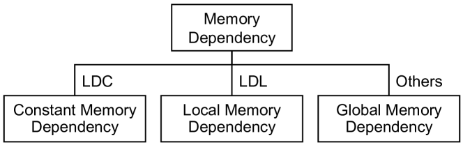
(a) Memory dependency

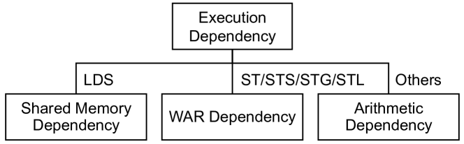
(b) Execution dependency

Figure 5. Classification of detailed dependency stall reasons

After attributing stalls to their sources, we further classify the stall reasons for execution and memory dependencies according to the opcode of each source instruction. As shown in Figure 5, we categorize memory dependency as local memory, constant memory, and global memory dependencies. Knowing where local memory stalls occur is important for register pressure analysis because it often indicates register spills. Likewise, we classify execution dependency as shared memory, arithmetic, and write-after-read (WAR) dependencies. WAR dependency happens when a variable latency def instruction reads a value from a register, and the use instruction writes the same register.

5. Performance Optimizers and Estimators

This section describes the implementation of performance optimizers and estimators.

5.1. Performance Optimizers

Performance optimizers take program structure and the analysis result from the instruction blamer. Each optimizer encodes rules to calculate matching stalls. In this way, we lift the job of associating stalls with optimizations from users to the advisor.

Table 2. A brief description of GPU optimizers in GPA.

Code Optimizers
	Stall Elimination
	Register Reuse	Match memory dependency stalls of local memory read/write instructions
	Strength Reduction	Match execution dependency stalls of long latency arithmetic instructions
	Function Split	Match instruction fetch stalls
	Fast Math	Match stalls in CUDA math functions
	Warp Balance	Match warp synchronization stalls
	Memory Transaction Reduction	Match global memory throttling stalls
	Latency Hiding
	Loop Unrolling	Match global memory and execution dependency stalls in loops
	Code Reordering	Match global memory and execution dependency stalls
	Function Inlining	Match stalls in device functions and their call sites
Parallel Optimizers
	Block Increase	Match if the number of blocks is less than the number of SMs
	Thread Increase	Match if occupancy is limited by the number of threads per block

We classify the available performance optimizers in GPA in Table 2. At a high level, we have parallel and code optimizers. Parallel optimizers check if we can increase the parallelism level to improve performance. For instance, the Block Increase optimizer investigates the potential of increasing the number of blocks. Code optimizers check if we can adjust code to improve the performance. Based on optimization methods, we further categorize the code optimizers as stall elimination and latency hiding optimizers. Stall elimination optimizers provide suggestions to reduce stalls; latency hiding optimizers suggest rearranging issue orders to overlap stall latency.

Each optimizer maintains a workflow to match instruction samples. The Loop Unrolling optimizer, for example, iterates through all the latency samples. It records a latency sample if it has either a memory dependency stall or an execution dependency stall, and the def and the use instructions are within the same loop. The optimizer suggests using pragma unroll annotation or manual unrolling for loops where the compiler fails to unroll automatically.

5.2. Performance Estimators

With performance optimizers, we associate optimization methods with stalls, whereas it is still unclear which methods have a better effect in terms of the given measurement data, program structure, and the underlying GPU architecture. Performance estimators take the matched stalls as input and estimate the speedups by modeling the GPU’s execution. The optimizers with top estimated speedups output their suggestions to the performance advice report. According to the categories of optimizers, we classify estimators as code optimization estimators and parallel optimization estimators.

5.2.1. Code Optimization Estimators

We first model the effect of the stall elimination optimizers. Suppose the total of number samples for a GPU kernel is $T$, and the matched samples for an optimizer is $M$. Stall elimination optimizers assume we at best eliminate all the stalls by modifying the code. We use Equation 2 to estimate the speedup of stall elimination optimizers $\mathcal{S}^{e}$.

(2) $$~{}\mathcal{S}^{e}=\frac{T}{T-M}$$

Latency hiding optimizers suppose we can at best eliminate latency samples by modifying code. Therefore, we can use Equation 3 to estimate the speedup of latency hiding optimizers $\mathcal{S}^{h}$, where $M^{L}$ is the number of matched latency samples.

(3) $$~{}\mathcal{S}^{h}=\frac{T}{T-M^{L}}$$

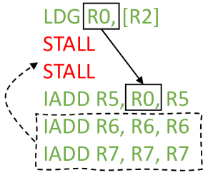
Figure 6. The mental model of latency hiding optimizers. Green code represents active samples, and red code represents latency samples. Latency hiding optimizers consider the effect of moving the code enclosed in dashed lines to fill stall slots.

Equation 3 models the execution at the kernel level. In practice, however, not all $M^{L}$ can be eliminated by rearranging code. Figure 6 explains the mental model of latency hiding optimization. We derive Equation 4 to refine the estimate of $\mathcal{S}^{h}$, where $A$ denotes the total number of active samples.

(4) $$~{}\mathcal{S}^{h}=\frac{T}{T-Min(A,M^{L})}$$

We prove that the upper bound of $\mathcal{S}^{h}$ is two. We use $L$ to denote the total number of latency samples, and $T=A+L$.

Theorem 5.1.

The speedup upper bound of latency hiding optimizations is 2$\times$.

Proof.

• If $Min(A,M^{L})=A$. $\frac{T}{T-A}=\frac{L+A}{(L+A)-A}=1+\frac{A}{L}$.
  Because $A\leq M^{L}\leq L,\frac{T}{T-Min(A,M_{L})}\leq 2$.

• If $Min(A,M^{L})=M^{L}$. $\frac{T}{T-M^{L}}=\frac{1}{1-\frac{M^{L}}{T}}=\frac{1}{1-\frac{M^{L}}{A+L}}$.
  Because $L\geq M^{L}$ and $A\geq M^{L}$, $\frac{M^{L}}{A+L}\leq\frac{1}{2}$.
  Then $\frac{T}{T-Min(A,M^{L})}\leq 2$.

∎

Scope Analysis

We observe that optimizations such as loop unrolling only arrange code for a specific scope so that only the active samples within the scope can be used to reduce latency samples. Based on this limitation, we propose Equation 5 to analyze optimization scopes representing loops and functions. $\mathcal{S}^{h}_{l}$ indicates the speedup for a specific scope $l$, and $M^{L}_{l}$ is the matched latency samples for a scope $l$.

(5) $$~{}\mathcal{S}^{h}_{l}=\frac{T}{T-Min(\sum\limits_{l^{\prime}\in nested(l)}A_{l^{\prime}},M^{L}_{l})}$$

Suppose we have a loop loop1 nested in another loop loop2, the speedup of of loop2 is bounded by the active samples of loop2 and loop1 according to Equation 5.

5.2.2. Parallel Optimization Estimator

Parallel optimizers adjust the number of blocks and threads within each block to change the parallelism level. To estimate the effect of adjusting blocks and threads, we take into account each warp scheduler’s change of active warps–$\mathcal{C}_{W}$ (Equation 6) and change of issue rate—$\mathcal{C}_{\mathcal{I}}$ (Equation 7) .

For instance, by increasing the number of blocks, we reduce the active warps per scheduler and $\mathcal{C}_{W}$ is less than one. If the number of threads of each block is reduced, the rate that a warp scheduler is issuing is reduced, and $\mathcal{C}_{\mathcal{I}}$ is less than one.

(6) $$~{}\mathcal{C}_{W}=\frac{W_{new}}{W}$$

(7) $$~{}\mathcal{C}_{\mathcal{I}}=\frac{\mathcal{I}_{new}}{\mathcal{I}}$$

Assuming every warp scheduler’s issue rate is the same across different SMs, we derive Equation 8 and Equation 9 to calculate $\mathcal{I}$ and $\mathcal{I}_{new}$ respectively, where $R_{I}$ is the ratio of issued samples among all samples. A warp scheduler is issuing if at least one warp on the scheduler is ready to issue an instruction.

(8) $$~{}\mathcal{I}=1-(1-R_{I})^{W}$$

(9) $$~{}\mathcal{I}_{new}=1-(1-R_{I})^{{W}_{new}}$$

(10) $$~{}\mathcal{S}^{p}=\frac{1}{\mathcal{C}_{W}}\times\mathcal{C}_{\mathcal{I}}\times f$$

Based on $\mathcal{C}_{W}$ and $\mathcal{C}_{\mathcal{I}}$, we estimate the speedup of parallel optimizations ($\mathcal{S}^{p}$) using Equation 10, where $f$ is a factor that varies between optimizers. Some optimizers may assume there is no pipeline, memory throttle, and no select stall if we reduce the number of active warps per block to a certain number (e.g., less than the number of schedulers per SM).

6. Evaluation

Table 3. Achieved speedups averaged among ten runs. We improved each code according to the suggestion provided by GPA. Estimate error is computed by $\frac{|Estimated\ Speedup-Achieved\ Speedup|}{Achieved\ Speedup}\times 100\%$

Application	Kernel	Optimization	Original	Achieved Speedup	Estimated Speedup	Error
rodinia/backprop	bpnn_layerforward_CUDA	Warp Balance	17.26$\pm$0.21us	1.15$\pm$0.03$\times$	1.14$\times$	1%
rodinia/backprop	bpnn_layerforward_CUDA	Strength Reduction	15.06$\pm$0.13us	1.21$\pm$0.01$\times$	1.24$\times$	2%
rodinia/bfs	Kernel	Loop Unrolling	567.14$\pm$2.04us	1.12$\pm$0.01$\times$	1.59$\times$	42%
rodinia/b+tree	findRangeK	Code Reorder	51.59$\pm$0.39us	1.16$\pm$0.1$\times$	1.28$\times$	10%
rodinia/cfd	cuda_compute_flux	Code Reorder	190.81$\pm$2.98ms	1.60$\pm$0.02$\times$	1.68$\times$	5%
rodinia/gaussian	Fan2	Thread Increase	105.76ms	3.58$\pm$0.15$\times$	3.32$\times$	7%
rodinia/heartwall	kernel	Loop Unrolling	94.06$\pm$2.79ms	1.17$\pm$0.03$\times$	1.18$\times$	1%
rodinia/hotspot	calculate_temp	Strength Reduction	11.92$\pm$0.08us	1.14$\pm$0.01$\times$	1.09$\times$	4%
rodinia/huffman	vlc_encode_kernel_sm64huff	Warp Balance	123.40$\pm$0.28us	1.07$\times$	1.17$\times$	9%
rodinia/kmeans	kmeansPoint	Loop Unrolling	784.41$\pm$4.81us	1.11$\pm$0.01$\times$	1.20$\times$	8%
rodinia/lavaMD	kernel_gpu_cuda	Loop Unrolling	4.04$\pm$0.04ms	1.11$\pm$0.03$\times$	1.12$\times$	1%
rodinia/lud	lud_diagonal	Code Reorder	218.33$\pm$0.11us	1.41$\times$	1.48$\times$	5%
rodinia/myocyte	solver_2	Fast Math	308.55$\pm$6.87ms	1.22$\pm$0.03$\times$	1.13$\times$	7%
rodinia/myocyte	solver_2	Function Splitting	258.09$\pm$0.27ms	1.02$\pm$0.01$\times$	1.01$\times$	1%
rodinia/nw	needle_cuda_shared_1	Warp Balance	839.11$\pm$0.80us	1.07$\pm$0.01$\times$	1.09$\times$	2%
rodinia/particlefilter	likelihood_kernel	Block Increase	2.05$\pm$0.02ms	1.75$\pm$0.01$\times$	1.92$\times$	10%
rodinia/streamcluster	kernel_compute_cost	Block Increase	20.73$\pm$0.28ms	1.52$\pm$0.03$\times$	1.35$\times$	11%
rodinia/sradv1	reduce	Warp Balance	1.94$\pm$0.28ms	1.02$\pm$0.01$\times$	1.10$\times$	8%
rodinia/pathfinder	dynproc_kernel	Code Reorder	94.60$\pm$0.68us	1.04$\pm$0.01$\times$	1.31$\times$	26%
Quicksilver	CycleTracking_Kernel	Function Inlining	50.48$\pm$0.70s	1.14$\pm$0.01$\times$	1.18$\times$	4%
Quicksilver	CycleTracking_Kernel	Register Reuse	50.07$\pm$0.86s	1.02$\pm$0.01$\times$	1.04$\times$	2%
ExaTENSOR	tensor_transpose	Strength Reduction	5.60$\pm$0.02ms	1.11$\pm$0.01$\times$	1.06$\times$	5%
ExaTENSOR	tensor_transpose	Memory Transaction Reduction	5.07$\pm$0.01ms	1.03$\times$	1.05$\times$	2%
PeleC	react_state	Block Increase	121.60$\pm$1.05s	1.21$\pm$0.01$\times$	1.23$\times$	2%
Minimod	target_pml_3d	Fast Math	88.88$\pm$1.14ms	1.03$\pm$0.01$\times$	1.09$\times$	6%
Minimod	target_pml_3d	Code Reorder	85.99$\pm$0.06ms	1.04$\pm$0.01$\times$	1.05$\times$	1%
average				1.22$\times$	1.26$\times$	4.1%

We evaluated GPA on an x86_64 system with two Intel E5-2695 processors and a single NVIDIA Volta v100 GPU. The following system software are used: Linux 3.10.0, NVIDIA CUDA Toolkit 11.0.194, NVIDIA Driver 450.51.06, and GCC 7.3.0. We evaluated GPA on Rodinia benchmarks and applications described below:

• Quicksilver (qui, 2020) is a proxy application that solves a dynamic Monte Carlo particle transport problem. Quicksilver has a single large kernel that invokes many device functions consisting of thousands of lines of code. We studied Quicksilver with its default input.

• ExaTENSOR (exa, 2020) is a library for large-scale numerical tensor algebra. We studied its tensor transpose kernel using a large six-dimensional tensor.

• PeleC (pel, 2020) is an application for reacting flows using adaptive-mesh compressible hydrodynamics. We studied PeleC using its default input.

• Minimod (Meng et al., 2020) is a benchmark application for seismic modeling. We analyzed its higher-order stencil codes using grid sizes of $100^{3}$.

Each row in Table 3 quantifies the speedup we achieved by applying the corresponding optimization suggested by GPA. For each benchmark, we focused on the dominant GPU kernel and implemented one of the top five optimization suggestions, based on its estimated speedup and ease of implementation. On average, we achieved a geometric mean of 1.22$\times$ speedup with individual speedups ranging from 1.01$\times$ to 3.53$\times$. GPA’s estimated speedup is close to the speedup we achieved, with a geometric mean of the gap between the speedup we achieved and the estimated speedup of 4.1%. In the rest of this section, we describe observations while analyzing and optimizing benchmarks using GPA, including the optimization workflow, false positivity, and single dependency coverage.

6.1. Optimization Workflow

Before using GPA, one can apply a source-to-source transformation to separate variables that appear on a single line. Then, one can start by interpreting the top optimizations in the advice report by GPA. Not all optimizations are easy to implement. For example, for a code reordering suggestion, if the distance between the def and use instructions is long, it is hard to improve it further. Based on our experience of studying benchmarks, one can investigate the problem, modify the code, and achieve speedup within half an hour. Typically, only a few lines need to be changed to achieve non-trivial speedups.

6.2. False Positivity

GPA could overestimate optimization opportunities. From Table 3, we observe that loop unrolling and code reordering optimizations have the highest estimate errors.

The overestimation of the benefits of loop unrolling occurs because the loop unrolling optimizer lacks information about the number of iterations and compiler information. After closely investigating the bfs benchmark, we found that the workload is highly unbalanced such that most threads only execute less than four iterations of the loop. Thus, loop unrolling benefits only a small number of threads.

The data dependency restriction causes the false positivity of code reordering optimization. GPA suggests reordering a global memory read in a loop of the pathfinder benchmark. The estimated speedup is 26% higher than we achieved because instructions after synchronizations depend on the results before synchronizations. Therefore, the instructions we can use to hide latency are limited in a fine-grained scope in which the distance between the dependent instruction pairs is short no matter how we arrange instructions.

6.3. Single Dependency Coverage

Figure 7. Single dependency coverage before and after pruning cold edges

In the instruction dependency graph, we say a node is a single dependency node if the node does not have any incoming edge, or each incoming edge represents a different dependency. We define single dependency coverage as the ratio of single dependency nodes to the total number of nodes. Figure 7 quantifies the single dependency coverage before and after pruning cold edges. After applying edge pruning heuristics, most benchmarks have single dependency coverage greater than 0.8 so that we can attribute the stalls to one edge without apportioning.

Two exceptions are the bfs and the nw benchmarks. The bfs benchmark is memory-intensive. Most of the instructions are global memory read/stores, which have a 64-bit memory address stored in two 32-bit registers. The nw benchmark has many nodes with multiple incoming edges because of its intricate control flow. The dominant loop in nw is fully unrolled. Within the loop, there is a condition that decides if values are calculated or not. If yes, it compares four candidates and chooses the maximum one.

7. Case Studies

In this section, we study the optimizations for the four larger benchmark codes in Table 3, including ExaTENSOR, Quicksilver, PeleC, and Minimod on the platform we mentioned in Section 6. The GPU code of the applications was compiled with -O3 -lineinfo. With the following case studies, we show that one can achieve non-trivial speedup without in-depth knowledge of the assembly code and the GPU architecture.

7.1. ExaTENSOR

Figure 8. A performance report for ExaTENSOR

We studied a tensor transpose kernel in ExaTENSOR. We show a part of GPA’s report in Figure 8. GPA ranks optimizers based on their estimated speedups. Each optimizer suggests a few methods to modify the code and lists several hotspots to focus on. Each hotspot consists of the def and use locations and their distance. In Figure 8, GPA reports that we can follow the suggestions of the strength reduction optimizer. Because the hotspot code performs an integer division, we can replace it with a multiplication by its reciprocal. This optimization renders a 1.11$\times$ speedup.

We analyzed the modified code again with GPA. This time GPA suggests a memory transaction reduction optimization to mitigate memory throttling stalls. In particular, GPA suggests that we replace global memory reads by constant memory reads if elements are shared between threads and not changed during execution. According to the suggestion, we achieved a 1.03$\times$ speedup.

7.2. Quicksilver

We used GPA to analyze Quicksilver on a single GPU. GPA reports the function inlining optimization may render the highest speedup. Applying the always_inline keyword for these functions fails to inline due to the size/register limitation forced by the compiler. Therefore, we manually inlined two small functions by integrating the whole function bodies into their callers. By modifying the code in this way, we obtained a $1.14\times$ speedup.

Next, GPA’s register reuse optimizer indicates local memory stalls in a loop and points out the potential cause of register spilling. GPA suggests splitting the loop into two to save registers. Without GPA, the raw PC sampling report by other tools only show global memory stalls without identifying register pressure. Applying the optimization yields a $1.01\times$ speedup.

7.3. PeleC

We studied the react_state kernel of PeleC. GPA estimates the code reordering optimization may result in the highest speedup. However, because the top five hotspots only account for 4 % all of the matched stalls, there are many hotspots distributed across lines so that it is difficult to adjust the code manually. The second best optimizer suggests increasing the number of blocks. Since the kernel only occupies 16 blocks, GPA suggests reducing the number of threads per block while increasing the number of blocks to improve the parallelism. By increasing the number of blocks to 32, we achieved a 1.21$\times$ speedup.

7.4. Minimod

We applied GPA to analyze the target_pml_3d kernel of Minimod, which performs higher-order multi-statement stencil computations. GPA first suggests using the fast math functions to replace high precision match functions. We applied the --use_fast_math compiler flag to achieve a 1.03$\times$ speedup.

Next, GPA suggests the code reordering optimizations for the updated code. Adjusting the code to read subscripted values from global memory well in advance of their use hides more of the memory latency and yields an additional 1.04$\times$ speedup.

8. Related Work

GPU profilers are widely available in various GPU architectures. NVIDIA provides several tools (nvp, 2019; NVIDIA Corporation, 2020c, b) to measure GPU performance metrics. Intel develops VTune (Reinders, 2005) to monitor executions on both CPUs and GPUs. AMD provides ROCProfiler (roc, 2020) to read hardware counters and trace applications. There are also tools (Zhou et al., 2020; Shende and Malony, 2006; Mey et al., 2012; Zhang, 2018; Zhang and Hollingsworth, 2019) that focus on large HPC applications. Among the above tools, NVIDIA’s nsight-compute provides the most information at the GPU kernel level. It characterizes GPU kernels’ bottlenecks at the high level but does not pinpoint bottlenecks and provide suggestions for specific code regions. In contrast, GPA analyzes control flow, program structure, architectural features, and interprets measurement data to provide thorough suggestions and estimate speedups.

GPU vendors have also developed instrumentation tools (Kambadur et al., 2015; Stephenson et al., 2015; Villa et al., 2019; NVIDIA Corporation, 2020a) for fine-grained performance measurement and analysis. These tools, however, introduce unavoidable overhead for GPU kernels. GPA adopts PC sampling (Corporation, 2019), which introduces considerably less cost for kernel execution. There have been efforts that use instrumentation methods to diagnose specific types of inefficiencies. Yeh et al.  (Braun and Fröning, 2019) instrument GPU code as it is generated by LLVM to identify redundant instructions. CUDAAdvisor (Shen et al., 2018) also instruments code as it is generated by LLVM to monitor GPU memory access and decide if bypassing could be used. GVProf (gvp, 2020) instruments GPU binaries to detect both temporal and spatial redundant value patterns. These tools only identify a particular type of inefficiencies and do not correlate the problem with hotness. In comparison, GPA performs a comprehensive analysis of stall reasons for instruction samples and derives various optimization suggestions for hot code regions.

On the CPU side, there exist several tools that examine code quality and provide optimization suggestions. PerfExpert (Burtscher et al., 2010) collects performance metrics using sampling, analyzes measurement data and system parameters, and estimates performance upper-bounds. AutoScope (Sopeju et al., 2011) extends PerfExpert to suggest optimization strategies based on the detected bottlenecks. Unlike these two tools, CQA (Charif-Rubial et al., 2014) builds a static model by emulating processor pipelines to check symptoms (e.g., vectorization) on the loop level. VTune (Yasin, 2014) uses structured guidance to characterize the bottlenecks by interpreting performance counters.

Profile-guided optimization takes measurement data as input to guide compiler perform code transformation. Practical Path Profiling (PPP) (Bond and McKinley, 2005) collects edge profiles using instrumentation to help compilers make decisions about function inlining and loop unrolling. Instrumentation-based methods require using representative inputs to dump meaningful profiles. To avoid the overhead of instrumentation-based approaches, AutoFDO (Chen et al., 2016) uses hardware counter based sampling to collect profiles for production applications and use the profiles to guide optimizations. While most profile-guided optimization tools attribute measurement data to source lines to provide feedback for compilers, BOLT (Panchenko et al., 2019) is a post link optimizer that attributes samples on machine instructions and uses this information to derive binary optimizations. Recently, there also has been research that incorporates machine learning to guide optimizations. Cavazos et al. (Cavazos et al., 2007) use profile data as input features to a regression model that predicts the best compiler flags. DeepFrame (Guha et al., 2019) incorporates deep learning methods to learn the most likely paths during execution and offload the regions to FPGAs. Though profiler-guided optimizations can automatically adjust code based on rules or models, they only cover a subset of all the available optimizations. Many optimizations on GPUs need manual effort, such as warp balance, memory coalescing, and adjustments to the thread counts. Unlike other tools, GPA depends only on line-mapping information and is not tied to any specific compiler.

9. Conclusions and Future Work

Tuning GPU kernels is difficult due to the complexity of GPU architectures and programming models. To free application developers from needing to interpret measurements from multiple performance counters and analyze program inefficiencies, we introduce GPA. This performance advisor provides insightful optimization advice at the levels of lines, loops, and kernels and estimates each optimization’s speedup. GPA is organized in a modular fashion. Users can add custom optimizers to match other inefficiency patterns (e.g., texture fetch combination).

GPA suffers from both hardware and software limitations. First, GPA apportions stalls to multiple dependency sources with an approximation method based on the instruction counts in the paths. If the underlying hardware implements “paired sampling” (Dean et al., 1997), we could collect precisely both the stalled instruction and the instruction that causes the stall. Second, to obtain a more accurate speedup estimate, comprehensive compiler information such as loop unroll count should be considered. Last, because PC Sampling with NVIDIA’s CUPTI serializes kernel executions, GPA’s profiler is unable to measure the effect of concurrent kernel execution.

In the future, we plan to ingest compiler information into GPA to perform a more accurate estimate. In addition, we can use the insights derived from GPA to guide compilers to apply code transformation for large-scale applications with hundreds of tiny hotspots.

References

- (1)
- nvp (2019) 2019. The user manual for NVIDIA profiling tools for optimizing performance of CUDA applications. https://docs.nvidia.com/cuda/profiler-users-guide [Accessed August 26, 2020].
- roc (2020) 2020. AMD ROCm ROCProfiler. https://rocmdocs.amd.com/en/latest/ROCm_Tools/ROCm-Tools.html [Accessed August 26, 2020].
- exa (2020) 2020. ExaTENSOR. https://iadac.github.io/projects/ [Accessed August 27th, 2020].
- gvp (2020) 2020. GVPROF: A Value Profiler for GPU-based Clusters. https://github.com/Jokeren/GVProf [Accessed August 26, 2020].
- pel (2020) 2020. PeleC. https://github.com/AMReX-Combustion/PeleC [Accessed August 27th, 2020].
- qui (2020) 2020. Quicksilver. https://github.com/LLNL/Quicksilver [Accessed August 26, 2020].
- Bond and McKinley (2005) Michael D Bond and Kathryn S McKinley. 2005. Practical path profiling for dynamic optimizers. In International Symposium on Code Generation and Optimization. IEEE, 205–216.
- Braun and Fröning (2019) Lorenz Braun and Holger Fröning. 2019. CUDA Flux: A Lightweight Instruction Profiler for CUDA Applications. In Performance Modeling, Benchmarking and Simulation of High Performance Computer Systems (PMBS) Workshop, collocated with International Conference for High Performance Computing, Networking, Storage and Analysis (SC2019).
- Burtscher et al. (2010) Martin Burtscher, Byoung-Do Kim, Jeff Diamond, John McCalpin, Lars Koesterke, and James Browne. 2010. Perfexpert: An easy-to-use performance diagnosis tool for hpc applications. In SC’10: Proceedings of the 2010 ACM/IEEE International Conference for High Performance Computing, Networking, Storage and Analysis. IEEE, 1–11.
- Cavazos et al. (2007) John Cavazos, Grigori Fursin, Felix Agakov, Edwin Bonilla, Michael FP O’Boyle, and Olivier Temam. 2007. Rapidly selecting good compiler optimizations using performance counters. In International Symposium on Code Generation and Optimization (CGO’07). IEEE, 185–197.
- Charif-Rubial et al. (2014) Andres S Charif-Rubial, Emmanuel Oseret, José Noudohouenou, William Jalby, and Ghislain Lartigue. 2014. CQA: A code quality analyzer tool at binary level. In 2014 21st International Conference on High Performance Computing (HiPC). IEEE, 1–10.
- Che et al. (2009) Shuai Che, Michael Boyer, Jiayuan Meng, David Tarjan, Jeremy W Sheaffer, Sang-Ha Lee, and Kevin Skadron. 2009. Rodinia: A benchmark suite for heterogeneous computing. In 2009 IEEE international symposium on workload characterization (IISWC). Ieee, 44–54.
- Chen et al. (2016) Dehao Chen, Tipp Moseley, and David Xinliang Li. 2016. AutoFDO: Automatic feedback-directed optimization for warehouse-scale applications. In 2016 IEEE/ACM International Symposium on Code Generation and Optimization (CGO). IEEE, 12–23.
- Cifuentes and Fraboulet (1997) Cristina Cifuentes and Antoine Fraboulet. 1997. Intraprocedural static slicing of binary executables. In 1997 Proceedings International Conference on Software Maintenance. IEEE, 188–195.
- Corporation (2019) NVIDIA Corporation. 2019. PC Sampling. https://docs.nvidia.com/cupti/Cupti/r_main.html#r_pc_sampling [Accessed January 26, 2019].
- Dean et al. (1997) Jeffrey Dean, James E Hicks, Carl A Waldspurger, William E Weihl, and George Chrysos. 1997. ProfileMe: Hardware support for instruction-level profiling on out-of-order processors. In Proceedings of 30th Annual International Symposium on Microarchitecture. IEEE, 292–302.
- Drongowski (2007) Paul J Drongowski. 2007. Instruction-based sampling: A new performance analysis technique for AMD family 10h processors. Advanced Micro Devices (2007).
- Guha et al. (2019) Apala Guha, Naveen Vedula, and Arrvindh Shriraman. 2019. Deepframe: A Profile-Driven Compiler for Spatial Hardware Accelerators. In 2019 28th International Conference on Parallel Architectures and Compilation Techniques (PACT). IEEE, 68–81.
- Guide (2011) Part Guide. 2011. Intel® 64 and ia-32 architectures software developer’s manual. Volume 3B: System programming Guide, Part 2 (2011), 11.
- January et al. (2015) Christopher January, Jonathan Byrd, Xavier Oró, and Mark O’Connor. 2015. Allinea MAP: Adding Energy and OpenMP Profiling Without Increasing Overhead. In Tools for High Performance Computing 2014. Springer, 25–35.
- Jia et al. (2018) Zhe Jia, Marco Maggioni, Benjamin Staiger, and Daniele P Scarpazza. 2018. Dissecting the nvidia volta gpu architecture via microbenchmarking. arXiv preprint arXiv:1804.06826 (2018).
- Kambadur et al. (2015) Melanie Kambadur, Sunpyo Hong, Juan Cabral, Harish Patil, Chi-Keung Luk, Sohaib Sajid, and Martha A Kim. 2015. Fast computational gpu design with gt-pin. In 2015 IEEE International Symposium on Workload Characterization. IEEE, 76–86.
- Meng et al. (2020) Jie Meng, Andreas Atle, Henri Calandra, and Mauricio Araya-Polo. 2020. Minimod: A Finite Difference solver for Seismic Modeling. arXiv preprint arXiv:2007.06048v1 (2020).
- Mey et al. (2012) Dieteran Mey, Scott Biersdorf, Christian Bischof, Kai Diethelm, Dominic Eschweiler, Michael Gerndt, Andreas Knapfer, Daniel Lorenz, Allen Malony, WolfgangE. Nagel, Yury Oleynik, Christian Rassel, Pavel Saviankou, Dirk Schmidl, Sameer Shende, Michael Wagner, Bert Wesarg, and Felix Wolf. 2012. Score-P: A Unified Performance Measurement System for Petascale Applications. In Competence in High Performance Computing 2010, Christian Bischof, Heinz-Gerd Hegering, Wolfgang E. Nagel, and Gabriel Wittum (Eds.). Springer Berlin Heidelberg, 85–97.
- NVIDIA Corporation (2019) NVIDIA Corporation. 2019. CUPTI User’s Guide DA-05679-001_v10.1. https://docs.nvidia.com/cuda/pdf/CUPTI_Library.pdf.
- NVIDIA Corporation (2020a) NVIDIA Corporation. 2020a. NVIDIA Compute Sanitizer. https://docs.nvidia.com/cuda/compute-sanitizer/index.html [Accessed August 26, 2020].
- NVIDIA Corporation (2020b) NVIDIA Corporation. 2020b. NVIDIA Nsight Compute. https://developer.nvidia.com/nsight-compute [Accessed August 26, 2020].
- NVIDIA Corporation (2020c) NVIDIA Corporation. 2020c. NVIDIA Nsight Systems. https://developer.nvidia.com/nsight-systems [Accessed August 26, 2020].
- of Wisconsin-Madison ([n.d.]) University of Wisconsin-Madison. [n.d.]. Dyninst. https://github.com/dyninst/dyninst [Accessed January 26, 2020].
- Panchenko et al. (2019) Maksim Panchenko, Rafael Auler, Bill Nell, and Guilherme Ottoni. 2019. Bolt: a practical binary optimizer for data centers and beyond. In 2019 IEEE/ACM International Symposium on Code Generation and Optimization (CGO). IEEE, 2–14.
- Reinders (2005) James Reinders. 2005. VTune performance analyzer essentials. Intel Press (2005).
- Shen et al. (2018) Du Shen, Shuaiwen Leon Song, Ang Li, and Xu Liu. 2018. Cudaadvisor: Llvm-based runtime profiling for modern gpus. In Proceedings of the 2018 International Symposium on Code Generation and Optimization. 214–227.
- Shende and Malony (2006) Sameer S Shende and Allen D Malony. 2006. The TAU parallel performance system. The International Journal of High Performance Computing Applications 20, 2 (2006), 287–311.
- Sopeju et al. (2011) Olalekan A Sopeju, Martin Burtscher, Ashay Rane, and James Browne. 2011. Autoscope: Automatic suggestions for code optimizations using perfexpert. Evaluation (2011).
- Srinivasan and Reps (2016) Venkatesh Srinivasan and Thomas Reps. 2016. An improved algorithm for slicing machine code. ACM SIGPLAN Notices 51, 10 (2016), 378–393.
- Stephenson et al. (2015) Mark Stephenson, Siva Kumar Sastry Hari, Yunsup Lee, Eiman Ebrahimi, Daniel R Johnson, David Nellans, Mike O’Connor, and Stephen W Keckler. 2015. Flexible software profiling of gpu architectures. In ACM SIGARCH Computer Architecture News, Vol. 43. ACM, 185–197.
- Villa et al. (2019) Oreste Villa, Mark Stephenson, David Nellans, and Stephen W Keckler. 2019. NVBit: A Dynamic Binary Instrumentation Framework for NVIDIA GPUs. In Proceedings of the 52nd Annual IEEE/ACM International Symposium on Microarchitecture. ACM, 372–383.
- Yasin (2014) Ahmad Yasin. 2014. A top-down method for performance analysis and counters architecture. In 2014 IEEE International Symposium on Performance Analysis of Systems and Software (ISPASS). IEEE, 35–44.
- Zhang (2018) Hui Zhang. 2018. Data-centric performance measurement and mapping for highly parallel programming models. Ph.D. Dissertation. University of Maryland—College Park.
- Zhang and Hollingsworth (2019) H. Zhang and J. Hollingsworth. 2019. Understanding the Performance of GPGPU Applications from a Data-Centric View. In 2019 IEEE/ACM International Workshop on Programming and Performance Visualization Tools (ProTools). 1–8. https://doi.org/10.1109/ProTools49597.2019.00006
- Zhang et al. (2017) Xiuxia Zhang, Guangming Tan, Shuangbai Xue, Jiajia Li, Keren Zhou, and Mingyu Chen. 2017. Understanding the gpu microarchitecture to achieve bare-metal performance tuning. In Proceedings of the 22nd ACM SIGPLAN Symposium on Principles and Practice of Parallel Programming. 31–43.
- Zhou et al. (2020) Keren Zhou, Mark W. Krentel, and John Mellor-Crummey. 2020. Tools for Top-down Performance Analysis of GPU-Accelerated Applications. In Proceedings of the 34th ACM International Conference on Supercomputing (ICS ’20). Association for Computing Machinery, New York, NY, USA, Article 26, 12 pages. https://doi.org/10.1145/3392717.3392752