Dielectric Skyrmions

Abstract

We consider the dielectric Skyrme model proposed recently, with and without the addition of the standard pion mass term. Then we write down Bogomol’nyi-type energy bounds for both the massless and massive cases. We further show that, except for when taking the strict BPS limit, the Skyrmions are made of 3 orthogonal dipoles that can always be placed in their attractive channel and form bound states. Finally, we study the model numerically and discover that, long before realistic binding energies are reached, the Skyrmions become bound states of well-separated point-particle-like Skyrmions. By going sufficiently close to the BPS limit, we are able to obtain classical binding energies of realistic values compared with experiments.

1 Introduction

The Skyrme model Skyrme:1961vq ; Skyrme:1962vh is an effective field theory with the symmetries of the strong interactions at low energies, much like chiral perturbation theory Weinberg:1978kz . Two main differences between the approaches of the Skyrme model and chiral perturbation theory lie in how the nucleon (baryon) is implemented and that some fine tuning between some coefficients is usually adopted in the Skyrme-type models. The implementation of the nucleon in chiral perturbation theory is simply done by means of a point-particle operator, as is standard in fundamental quantum field theory, whereas in the Skyrme-model approach, the nucleon is a topological soliton in the pion fields. Clearly, taking the nucleon to be a point particle, is just an approximation, but for many purposes a quite good one at sufficiently low energies. The higher the energies are for the questions one is asking, the worse it gets of course. The other difference mentioned above, is that in chiral perturbation theory, several operators at $p^{4}$ (fourth order in derivatives) include four time derivatives, and in the Skyrme model it is customary to take the coefficients of said operators such that the four time derivatives cancel out, exactly. This is a matter of practicality as it makes it possible to quantize the spin and isospin zero modes by means of a standard Hamiltonian analysis.

Serious attention was first given to the Skyrme model after Witten pointed out that the baryon in large-$N$ QCD (Quantum Chromodynamics) should be identified with the Skyrmion Witten:1983tw ; Witten:1983tx . In particular, Adkins–Nappi–Witten provided the basis upon which many papers could continue the investigation of the Skyrme model as a model of the nucleon Adkins:1983ya , see the review Zahed:1986qz . The first obstacle of studying nuclei beyond the single nucleon was to obtain solutions to the full partial differential equations (PDEs), being the equations of motion (EOM) of the Skyrme model, without spherical symmetry restrictions. This was overcome by Battye and Sutcliffe by means of the rational map approximation (RMA) and shell-like fullerenes of Skyrmions were obtained Battye:1997qq . It was now clear that we were faced with a new problem: the binding energies of the Skyrmions were far too large compared to those of nuclei. That is, typical binding energies in the Skyrme model are of the order of 10% per nucleon (Skyrmion), which should be compared to about 1% for real world nuclei. This binding-energy problem has been a theme in Skyrmion research for the last 20+ years.

The main tool for addressing the binding-energy problem is to write down a topological energy bound or Bogomol’nyi bound for the static energy of the model at hand Harland:2013rxa ; Adam:2013tga . Such a bound exists for the standard (massless) Skyrme model and is called the Skyrme–Faddeev bound Skyrme:1962vh ; Faddeev:1976pg and reads $E\geq 12\pi^{2}|B|$, where $B$ is the topological degree or baryon number. The energy bound, unfortunately, cannot be saturated by Skyrmions on flat space, although it can be saturated by a Skyrmion on the 3-sphere, as shown by Manton and Ruback Manton:1986pz . The Skyrmion with baryon number $B$ will be denoted as a $B$-Skyrmion throughout the paper. The 1-Skyrmion has an energy that is about 23% above the Faddeev-Skyrme bound. Now let us assume that the $B$-Skyrmion is bound. This means that its energy divided by $B$ is smaller than 23% over the bound. The $B$-Skyrmion with the largest possible binding energy would thus correspond to the situation that it exactly saturates the bound. This means that the closeness of the 1-Skyrmion to the energy bound sets an upper limit on how large the binding energies can be for multi-Skyrmions (i.e. Skyrmions with $B>1$).

The above facts thus invited the community to a hunt for Skyrme-type models that either have a saturable energy bound or have Skyrmion solutions that can be quite close to the bound in some part of the parameter space. We shall use the expressions: energy bound, Bogomol’nyi bound and BPS bound interchangeably throughout the paper. The models that achieve the above-stated goal can be classified into 3 different categories: (1) models that have an attainable BPS bound for all topological charge sectors $B$; (2) models that have an attainable BPS bound only for the $B=1$ Skyrmion (with spherical symmetry); (3) models that have an asymptotic series of terms, which when all added up, hypothetically provide a model with an attainable BPS bound.

In the first category of models attempting to solve the binding-energy problem, there is only the BPS-Skyrme model Adam:2010fg ; Adam:2010ds by Adam–Sanchez-Guillen–Wereszczynski, which is a radical modification of the Skyrme model. That is, the Skyrme model Lagrangian is replaced by a different Lagrangian containing only a sixth-order derivative term, which is the baryon charge density (current) squared, as well as a suitable potential. This model has Skyrmion solutions of all topological degrees saturating the BPS bound. Although it may seem a radical and perhaps almost contrived step to replace the well-known terms of the chiral Lagrangian, this model has been shown to be equivalent to the small ’t Hooft coupling limit of the Sakai-Sugimoto model Sakai:2004cn , where the (holographic) Skyrmions become large and fluid-like due to a dominating sextic derivative term Bartolini:2017sxi . It is, however, questionable that the known solutions with $B>1$ are good candidates for near-BPS solutions, see ref. Speight:2014fqa for the notion of restricted harmonicity and ref. Gudnason:2020tps for near-BPS solutions in the 2-dimensional baby Skyrme model Leese:1989gi ; Piette:1994jt ; Piette:1994ug , which is a toy model for the Skyrme model.

In the second category, there is a Skyrme-type model made of the Skyrme term and the pion mass term to the fourth power Harland:2013rxa , which was indeed proposed by Harland due to the existence of a saturable energy bound that was found using the Hölder inequality. Being in the second category, it has a Skyrmion solution that saturates the energy bound, but only for $B=1$. This has the imminent repercussion that all $B>1$ solutions are unbound. Nevertheless, small perturbations of the model can quickly remedy this problem and provide a model of multi-Skyrmions with very low binding energies Gillard:2015eia , which was proposed by Gillard–Harland–Speight. A modification of the Gillard–Harland–Speight model was proposed by the author Gudnason:2016mms ; Gudnason:2016cdo ; Gudnason:2016tiz ; Gudnason:2018jia , where instead of the potential $(1-n_{0})^{4}$, the potential $(1-n_{0})^{2}$ was used, which has the effect of letting the Skyrmions possess larger discrete symmetries with lower binding energies, compared to the model of Gillard–Harland–Speight. Of course, for large enough potential coefficient, both models reduce to the point-particle model of Skyrmions Gillard:2016esy . This limit, incidentally is physically equivalent to the large ’t Hooft coupling limit of holographic Skyrmions in the Sakai-Sugimoto model Baldino:2017mqq . Another model in the second category is made by introducing field dependence to the coupling constants and is called the dielectric Skyrme model Adam:2020iye by Adam–Oles–Wereszczynski, which is a special case of the Ferreira model Ferreira:2017bsr where the coupling constants are promoted from scalars to field-space matrices (i.e. the diagonal identity matrix with a scalar function thus reduces to the latter model). These models can be viewed as special cases in the framework put forward in ref. Adam:2013hza . A very similar model has been proposed by Ferreira–Shnir Ferreira:2017yzy and Naya–Oles Naya:2020qvx , where the coupling constants are not functions of the fields, but of spatial coordinates, which is in the spirit of the inclusion of impurities Tong:2013iqa . Models with field dependent coupling constants, have long been considered, especially in the field of vortices, see e.g. refs. Bazeia:2010wr ; Bazeia:2012uc ; Bazeia:2012ux for a few first examples.

In the third category, there is the Sutcliffe model which is similar in spirit to holographic QCD in that it derives from a Yang-Mills action in five dimensions Sutcliffe:2010et ; Sutcliffe:2011ig . The main conceptual difference between the Sutcliffe model and a holographic model like the Sakai-Sugimoto model Sakai:2004cn , is that the latter has a scale – the curvature of anti-de Sitter space, which is translated via the holographic dictionary to the QCD scale (which in turn is defined as where the running gauge coupling of QCD becomes nonperturbative). Upon dimensional reduction from 5 dimensions to 4 dimensions, the Yang-Mills theory can be written as the Skyrme model – with coefficients fixed by the “background” – coupled to an infinite tower of vector mesons, just like in the Sakai-Sugimoto model. The missing gap in the Sutcliffe model is induced by truncating the infinite tower of vector mesons to a finite number and re-calibrating the units, whereas in the Sakai-Sugimoto model, it is an intrinsic quantity. The beauty of the Sutcliffe model, is that it explains why the instanton holonomy construction of Atiyah–Manton works so well. That is, in the limit of including the entire tower of vector mesons, the instanton holonomy description of the Skyrmion becomes exact. Unfortunately, in this limit the theory also loses its intrinsic mass scale, but it does become a BPS theory – Yang-Mills theory in 5 dimensions. In this sense, this model belongs to the third category; only when an infinite tower of vector mesons is taken into account, the theory becomes a BPS theory and hence has solutions that saturate the Bogomol’nyi bound.

Apart from the BPS race, some noteworthy studies of other aspects of physics, in particular of nuclear spectra, have been carried out. First, however, the importance of the pion mass for Skyrmion solutions with $B\gtrsim 12$ was recognized, which ruled out the shell-like fullerene structures as Skyrmion solutions for large atomic numbers Battye:2004rw ; Battye:2006tb ; Houghton:2006ti . This led to the conclusion that smaller “shells” must be preferred energetically, which turned out to be $B=4$ cubes happily overlapping with the alpha particle model of nuclei Battye:2006na . Zeromode quantization of the classical Skyrmion solution, using the rigid-body quantization put forward by Atkins–Nappi–Witten enjoyed some success for light nuclei, but mostly so for even atomic numbers (bosonic states) Battye:2009ad ; Lau:2014baa . It turns out that in order to even get the ground state right for the $B=7$ Skyrmion – identified with lithium-7/beryllium-7 – vibrational modes have to be included in the low-energy spectrum Halcrow:2015rvz , thus proving the insufficiency of restricting to zeromode quantization. Vibrational quantization was then tailored to specific nuclei with quite some success, based judiciously on constructed toy models with the right symmetries. This was done for carbon-12 Rawlinson:2017rcq , and oxygen-16 Halcrow:2016spb ; Halcrow:2019myn . A further important effect was discovered, namely that it is not enough to simply include both zeromodes and massive (vibrational) modes of the Skyrmion in a quantization scheme, but mixing between them leads to the crucial Coriolis effect Rawlinson:2019xsn , which improved the spectra for $B=4$ and $B=7$. Finally, a systematic investigation of the low-energy vibrational modes of Skyrmions with $B=1$ through $B=8$ was carried out Gudnason:2018ysx , laying the ground work for the development of a better quantization scheme.

In this paper, we will study the classical solutions of another variant of the Skyrme models that can be pushed close to a Bogomol’nyi bound, namely the dielectric Skyrme model Adam:2020iye mentioned above. It is the model where the coupling constants, i.e. the pion decay constant, $F_{\pi}$, and the Skyrme coupling $e_{\rm Skyrme}$, are promoted from constants (or running constants) to functions with field dependence. It is easy to find the correct form of the product of the two coupling functions, which unfortunately tends to zero in the vacuum in the BPS limit. It is unfortunate, because $e_{\rm Skyrme}=0$ makes the Skyrme term ill-defined and as well known this term (if not other higher-derivative terms are added to the Lagrangian) is a necessity for stabilizing the size of the Skyrmion due to Derrick’s theorem Derrick:1964ww . As for $F_{\pi}=0$ in the vacuum, this makes the pions nonpropagating in the vacuum and hence physically not acceptable. The damage is not too severe, since we do not want a BPS model anyway, we just want to move sufficiently close to such a limit, and hence we will consider the proposal by Adam–Oles–Wereszczynski to freeze the pion decay constant during its descent Adam:2020iye , such that it attains a finite value in the vacuum – thus allowing pions to propagate. Of course, there is some arbitrariness in how the freezing is done, but we will just stick to the simplest possibility in this paper.

At this point we have summarized, in quite some detail, some of the efforts that have been made for pushing the Skyrme program towards a working framework for low-energy nuclear physics. It would be illuminating at this point to pause and consider what we are trying to do in more abstract terms. We assume that the standard model of particle physics describes all known baryonic matter and its interactions. The most crucial ingredient is QCD, which is a Yang-Mills theory with gauge group SU(3). The particles charged under SU(3) of the strong interactions, are the quarks and the gluons (gauge fields of SU(3)). QCD has the unfortunate feature of possessing asymptotic freedom, which means that perturbation theory can be utilized only at large energies (say above 10 GeV or higher) and is useless at the QCD scale (about 250 MeV), below which the spectra of nuclei have to be extracted. The approach we take is called effective field theory, and in principle it is clear what has to be done. We should identify the scale at which we are interested in asking our questions and which particles are the low-energy degrees of freedom and further what symmetries they possess. The answer is also clear. Energies less than 10-20 MeV would be sufficient, and the symmetry and particle content is $\mathop{SU}\nolimits(2)_{L}\times\mathop{SU}\nolimits(2)_{R}$ chiral symmetry and pions, respectively. Now the recipe is simple, write down all possible symmetry-preserving operators in the Lagrangian up a high enough order in mass-dimension. The difficulty is that the pions were not in the QCD Lagrangian to begin with, but are composite particles made of two quarks in a bound state – bound by gluons. Therefore, we do not know how to determine the coefficients of the operators in the chiral Lagrangian from a theoretical point of view, they must be determined experimentally – hence with experimental uncertainties. The other problem arises due to the nature of using a soliton to describe the nucleon. That is, the soliton is an extended field configuration that even in the ground state has nonvanishing field derivatives. This makes it difficult to justify any order (in mass dimension or in derivatives) to which we may truncate the effective theory, and hence motivates a theory with an infinite number of terms (for a guess see refs. Marleau:1989fh ; Marleau:1991jk ; Marleau:2000ia ). It is, nevertheless, plausible that resummations of terms are possible in certain sectors and that due to such resummations, the infinite tower of operators can – at least approximately – be written as a sum of geometric series multiplying fundamental operators of the Lagrangian. Such a wild-eyed philosophy is what we will offer as a justification for allowing the coupling constants to be functions of the fields of the model.

The paper is organized as follows. The dielectric Skyrme model is reviewed in sec. 2 and its Bogomol’nyi bound in sec. 2.1. The near-BPS version of the model is described in sec. 2.2, the inclusion of the pion mass term in sec. 2.3 and the modification of the energy bound due to the pion mass term in sec. 2.3.1. Then the equations of motion are studied in sec. 2.4 and linearized to reveal the single Skyrmion as 3 orthogonal dipoles, which can attract another Skyrmion in the attractive channel in the entire parameter space of the near-BPS model, see sec. 2.5. The numerical results are presented in sec. 3 and finally the paper is concluded in sec. 4 with a discussion.

2 The dielectric Skyrme model

We consider the model Adam:2020iye

$$\mathcal{L}=\frac{f^{2}}{2}\mathop{tr}\nolimits(L_{\mu}L^{\mu})+\frac{1}{16e^{2}}\mathop{tr}\nolimits\left([L_{\mu},L_{\nu}][L^{\mu},L^{\nu}]\right),$$ (1)

with $f=f(\mathop{tr}\nolimits U/2)$ and $e=e(\mathop{tr}\nolimits U/2)$ being dimensionless functions, we have defined the left-invariant chiral current

$$L_{\mu}\equiv U^{\dagger}\partial_{\mu}U,$$ (2)

the field $U$ takes value in $\mathop{SU}\nolimits(2)$ and is related to an $\mathop{O}\nolimits(4)$-vector ${\mathbf{n}}=(n_{0},n_{1},n_{2},n_{3})$ by

$$U=n_{0}\mathbf{1}_{2}+\mathrm{i}\tau^{a}n_{a},\qquad a=1,2,3,$$ (3)

where $(n_{1},n_{2},n_{3})$ are known in physics as pions and $\tau^{a}$ are the Pauli matrices. The spacetime indices $\mu,\nu$ run over $0,1,2,3$ and we use the flat Minkowski metric of the mostly-positive signature. The model as written in eq. (1) is already in Skyrme units, where energy is measured in units of $F_{\pi}/(4e_{\rm Skyrme})$ and lengths are measured in units of $2/(F_{\pi}e_{\rm Skyrme})$, with $F_{\pi}$ the pion decay constant and $e_{\rm Skyrme}$ the Skyrme coupling Manton:2004 .

The functions $f$ and $e$ explicitly break the symmetry from $\mathop{SU}\nolimits(2)\times\mathop{SU}\nolimits(2)$ down to $\mathop{SU}\nolimits(2)$ (diagonal or vectorial). The theory is ungauged and therefore the requirement of finite energy configurations amounts to enforcing $\partial_{\mu}U=0$ at spatial infinity, which in turn effectively point compactifies 3-space from $\mathbb{R}^{3}$ to $\mathbb{R}^{3}\cup\{\infty\}\simeq S^{3}$. $\mathop{SU}\nolimits(2)$ viewed as a manifold is isomorphic to $S^{3}$ and hence the theory is characterized by the topological degree

$$\pi_{3}(S^{3})=\mathbb{Z}\ni B,$$ (4)

where $B$ is the degree of the mapping $U$ and is identified with the number of baryons. The topological degree can be directly calculated as

$$B=-\frac{1}{24\pi^{2}}\int_{\mathbb{R}^{3}}\epsilon_{ijk}\mathop{tr}\nolimits(L_{i}L_{j}L_{k})\;\mathrm{d}^{3}x,$$ (5)

where $i,j,k$ are spatial indices and thus run only over $1,2,3$ and we adopt the convention $\epsilon_{123}=+1$.

2.1 Bogomol’nyi bound

The static energy can be written as

$$E =\int_{\mathbb{R}^{3}}\mathop{tr}\nolimits\left[-\frac{f^{2}}{2}L_{i}L_{i}-\frac{1}{16e^{2}}[L_{i},L_{j}]^{2}\right]\mathrm{d}^{3}x$$

$$=\int_{\mathbb{R}^{3}}\mathop{tr}\nolimits\left[-\frac{1}{2}\left(fL_{i}\mp\frac{1}{2e}\epsilon_{ijk}L_{j}L_{k}\right)^{2}\mp\frac{f}{2e}\epsilon_{ijk}L_{i}L_{j}L_{k}\right]\mathrm{d}^{3}x,$$ (6)

where we have performed a Bogomol’nyi completion in the second line. The BPS equations are thus

$$L_{i}=\pm\frac{1}{2fe}\epsilon_{ijk}L_{j}L_{k},$$ (7)

yielding (anti-)Skyrmions for the upper (lower) sign. The fact that the cross term (last term) in the last line of the static energy (6) is proportional to the topological degree – even for $f$ and $e$ generalized to functions of $\tfrac{1}{2}\mathop{tr}\nolimits U$ – is due to the fact that they are target space functions. This can be seen as follows. Rewriting the expression for the topological degree (5), we have

$$B =-\frac{1}{24\pi^{2}}\int_{\mathbb{R}^{3}}\epsilon_{ijk}\mathop{tr}\nolimits(U^{\dagger}\partial_{i}UU^{\dagger}\partial_{j}UU^{\dagger}\partial_{k}U)\;\mathrm{d}^{3}x$$

$$=\frac{1}{12\pi^{2}}\int_{\mathbb{R}^{3}}\epsilon_{ABCD}\epsilon_{ijk}\,n_{A}\partial_{i}n_{B}\partial_{j}n_{C}\partial_{k}n_{D}\;\mathrm{d}^{3}x$$

$$=\int_{\mathbb{R}^{3}}{\mathbf{n}}^{*}\mathop{vol}\nolimits_{S^{3}}=B\int_{S^{3}}\mathop{vol}\nolimits_{S^{3}},$$ (8)

where the indices $A,B,C,D$ run over $0,1,2,3$, we use the convention $\epsilon_{0123}=+1$ and the normalized volume form on $S^{3}$ is denoted by $\mathop{vol}\nolimits_{S^{3}}$. The topological degree is simply the pullback of the volume form on $S^{3}$ to $\mathbb{R}^{3}$ by the field (map) ${\mathbf{n}}$ (or equivalently $U$), denoted by ${\mathbf{n}}^{*}$.

The integral of the cross term in the static energy (6) after Bogomol’nyi completion, can thus be written as

$$E_{\rm BPS} =\pm 12\pi^{2}\int_{\mathbb{R}^{3}}\frac{f(n_{0})}{e(n_{0})}{\mathbf{n}}^{*}\mathop{vol}\nolimits_{S^{3}}$$

$$=12\pi^{2}|B|\int_{S^{3}}\frac{f(n_{0})}{e(n_{0})}\mathop{vol}\nolimits_{S^{3}},$$ (9)

which can be interpreted as the target-space average of the function $f/e$ on the 3-sphere Adam:2020iye .

The BPS equation (7) can be solved only for $B=1$ Adam:2020iye , for which we can employ a hedgehog Ansatz

$$U=\cos\xi(r)\mathbf{1}_{2}+\mathrm{i}\tau^{a}\hat{x}^{a}\sin\xi(r),\qquad a=1,2,3,$$ (10)

where we have defined $\hat{x}^{a}=x^{a}/r$ with $r=\sqrt{x^{a}x^{a}}$. The left-invariant thus reads

$$L_{i}=\mathrm{i}\tau^{i}\frac{\sin 2\xi}{2r}+\mathrm{i}\hat{x}^{i}\hat{x}^{a}\tau^{a}\left(\xi^{\prime}-\frac{\sin 2\xi}{2r}\right)-\mathrm{i}\epsilon^{iab}\hat{x}^{a}\tau^{b}\frac{\sin^{2}\xi}{r},$$ (11)

which is the left-hand side of the BPS equation (7), whereas the right-hand side, being the commutator of $L_{j}$ and $L_{k}$, reads

$$\pm\frac{1}{fe}\left(-\mathrm{i}\tau^{i}\frac{\sin 2\xi}{2r}\xi^{\prime}+\mathrm{i}\hat{x}^{i}\hat{x}^{a}\tau^{a}\left[\frac{\sin 2\xi}{2r}\xi^{\prime}-\frac{\sin^{2}\xi}{r^{2}}\right]+\mathrm{i}\epsilon^{iab}\hat{x}^{a}\tau^{b}\frac{\sin^{2}(\xi)\xi^{\prime}}{r}\right),$$ (12)

which yields

$$\xi^{\prime}=\mp fe,\qquad fe\xi^{\prime}=\mp\frac{\sin^{2}\xi}{r^{2}},$$ (13)

where the former equation is obtained from all three tensor structures and the latter comes from the second tensor structure. Using the former equation in the latter, we thus get

$$(\xi^{\prime})^{2}=\frac{\sin^{2}\xi}{r^{2}}.$$ (14)

Taking the square root and choosing the negative sign and choosing the upper sign in eq. (13), we have

$$\xi^{\prime}=-fe,\qquad\xi^{\prime}=-\frac{\sin\xi}{r},$$ (15)

whose common solution with the appropriate boundary conditions $\xi(0)=\pi$ and $\xi(\infty)=0$ reads

$$\xi=2\arctan\frac{r_{0}}{r},\qquad fe=\frac{1}{r_{0}}(1-\cos\xi).$$ (16)

This is exactly the $B=1$ BPS solution found in ref. Adam:2020iye . Since the vacuum of the theory lies at $\xi=0$ or equivalently $U=\mathbf{1}_{2}$, the product $fe$ vanishes in the vacuum in the BPS limit. In terms of ${\mathbf{n}}$, we have

$$f(n_{0})e(n_{0})=\frac{1}{r_{0}}(1-n_{0}).$$ (17)

Obviously, we cannot allow $e(n_{0})$ to tend to zero, as that will make the Skyrme term ill defined in the vacuum. We would also like $f(n_{0})$ to take a nonvanishing value in the vacuum so as to conform with the physics of perturbative pions, far from the cores of nuclei. This leads us to the consideration of a near-BPS model.

2.2 Near-BPS dielectric Skyrme model

The near-BPS version we will study in this paper is based on freezing $f(n_{0})$ at a finite value before $n_{0}$ reaches the vacuum value $n_{0}=n_{0}^{\rm vac}=1$ Adam:2020iye . This will also allow us to introduce the normal pion mass term as a secondary (additional) BPS breaking term, without facing the problem of infinitely heavy pions.

The massless near-BPS version of the model in ${\mathbf{n}}$ coordinates reads

$$\mathcal{L}=-f^{2}(n_{0})\partial_{\mu}{\mathbf{n}}\cdot\partial^{\mu}{\mathbf{n}}-\frac{1}{2}(\partial_{\mu}{\mathbf{n}}\cdot\partial^{\mu}{\mathbf{n}})^{2}+\frac{1}{2}(\partial_{\mu}{\mathbf{n}}\cdot\partial_{\nu}{\mathbf{n}})(\partial^{\mu}{\mathbf{n}}\cdot\partial^{\nu}{\mathbf{n}}),$$ (18)

where we have fixed the coupling functions of the model as

$$f(n_{0})=\begin{cases}\frac{1-n_{0}+\beta}{1-n_{\star}+\beta},&n_{0}<n_{\star},\\ 1,&n_{0}\geq n_{\star},\end{cases}\qquad e(n_{0})=1,$$ (19)

with $\beta>0$ a positive constant.

This model has the nice feature that we can interpolate between the standard (massless) Skyrme model, i.e. for $n_{\star}=-1$, and the BPS model, i.e. for $n_{\star}=1$. In the standard Skyrme model, the Skyrmions are too strongly bound, whereas in the BPS limit there are only $B=1$ solutions that saturate the BPS bound, which in turn implies that all $B>1$ Skyrmions are unstable. We can therefore interpolate between a model that is too strongly bound and a model that is unbound. Somewhere in between $n_{\star}\in(-1,1)$ there may be realistic values for the binding energies of the multi-Skyrmions. What properties they have is what we want to study in this paper.

We can now exclude the possibility of going strictly to the BPS limit and therefore allow $n_{\star}\in[-1,1)$ only and hence

$$f(n_{0})=\begin{cases}\frac{1-n_{0}}{1-n_{\star}},&n_{0}<n_{\star},\\ 1,&n_{0}\geq n_{\star},\end{cases}\qquad e(n_{0})=1,$$ (20)

where we have set $\beta=0$. The normalization by $(1-n_{\star})$ is practical for making sure the Skyrmions do not grow to unreasonable sizes (which is impractical for numerical calculations).

We can now calculate the Bogomol’nyi bound (9) for the specific functions (20):

$$E_{\rm BPS} =12\pi^{2}|B|\left(\int_{S^{3}|n_{0}<n_{\star}}\frac{1-n_{0}}{1-n_{\star}}\mathop{vol}\nolimits_{S^{3}}+\int_{S^{3}|n_{0}\geq n_{\star}}\mathop{vol}\nolimits_{S^{3}}\right)$$

$$=12\pi^{2}|B|\left(\frac{2}{\pi(1-n_{\star})}\int_{\arccos(n_{\star})}^{\pi}2\sin^{2}\left(\frac{\xi}{2}\right)\sin^{2}\xi\;\mathrm{d}\xi+\frac{2}{\pi}\int_{0}^{\arccos(n_{\star})}\sin^{2}\xi\;\mathrm{d}\xi\right)$$

$$=12\pi^{2}|B|\mathcal{F}(n_{\star}),$$ (21)

where we have defined the function

$$\mathcal{F}(n_{\star})\equiv\frac{(2+n_{\star}^{2})\sqrt{1-n_{\star}^{2}}+3(\pi-n_{\star}\arccos(n_{\star}))}{3\pi(1-n_{\star})}.$$ (22)

The above defined function obeys $\mathcal{F}(-1)=1$, whereas in the limit $\lim_{n_{\star}\to 1^{-}}\mathcal{F}(n_{\star})\to\infty$, it diverges. This will not pose a problem, as we will not attempt at reaching the BPS limit.

Figure 1: The functional behavior $\mathcal{F}(n_{\star})$ of the Bogomol’nyi bound (21) in the massless case. The points (pluses) for every $n_{\star}\in\mathbb{Z}/10$, correspond to numerical solutions in later sections.

The function $\mathcal{F}(n_{\star})$ is shown in fig. 1.

It will prove convenient to define an energy functional, that is divided by the Bogomol’nyi bound

$$\epsilon_{B}\equiv\frac{E}{12\pi^{2}|B|\mathcal{F}(n_{\star})},$$ (23)

which holds for the massless near-BPS dielectric Skyrme model.

2.3 Including the pion mass term

Although the near-BPS model discussed in the previous section, has the aesthetically nice feature that we can interpolate between the standard massless Skyrme model and a BPS theory, we do want to break the BPS-ness. Hence introducing the standard pion mass term is not a problem. However, this means that we interpolate between the standard massive Skyrme model and another near BPS-model, so it is no longer guaranteed that we will reach low binding energies of multi-Skyrmions. Nevertheless, it is a straightforward numerical exploration and we will thus add to the near-BPS dielectric model the mass term

$$V=m^{2}\mathop{tr}\nolimits(\mathbf{1}_{2}-U)=2m^{2}(1-n_{0}),$$ (24)

which is the standard normalization and the pion mass parameter is often taken to be $m=1$ in Skyrme units Battye:2006na . Notice that because of our normalization of $f(n_{0})$ such that $f(n_{0})=1$ in the pion vacuum, the pion mass term is correctly normalized in this massive version of the near-BPS model.

2.3.1 Energy bound

Including the pion mass term alters the bound on the energy. In order to derive the bound, we first use the result of Harland Harland:2013rxa , for a submodel

$$E^{04}=\int_{\mathbb{R}^{3}}\left[-\frac{1}{16}\mathop{tr}\nolimits\big{(}[L_{i},L_{j}]^{2}\big{)}+V\right],$$ (25)

which reads Harland:2013rxa

$$E^{04}\geq 8\pi^{2}|B|\langle V^{1/4}\rangle,\qquad\langle V^{1/4}\rangle\equiv\int_{S^{3}}V^{1/4}\mathop{vol}\nolimits_{S^{3}},$$ (26)

where we have set $e=1$. Writing now the energy as

$$E=\int_{\mathbb{R}^{3}}\left[-\frac{f^{2}}{2}\mathop{tr}\nolimits(L_{i}L_{i})-\frac{1-\alpha+\alpha}{16}\mathop{tr}\nolimits\big{(}[L_{i},L_{j}]^{2}\big{)}+V\right],$$ (27)

and following refs. Harland:2013rxa ; Adam:2013tga , we get a combined bound

$$E\geq 12\pi^{2}|B|\mathcal{G},\qquad\mathcal{G}\equiv\langle f\rangle\left(\sqrt{\alpha}+\frac{2}{3\sqrt{a}}(1-\alpha)^{3/4}\right),\qquad a\equiv\frac{\langle f\rangle^{2}}{\langle V^{1/4}\rangle^{2}}>0,$$ (28)

which is a combined bound of eq. (9) for the massless dielectric Skyrme model and of eq. (26) for the submodel (25). The parameter $\alpha\in[0,1]$ is a weight of how much of the Skyrme term is used in the normal Skyrme-Faddeev bound and how much is used in the bound for the submodel (25).

The bound should be maximized by varying $\alpha$, which yields Adam:2013tga

$$\widehat{\alpha}=\frac{a^{2}}{2}\left(\sqrt{1+\frac{4}{a^{2}}}-1\right).$$ (29)

Keeping $\langle f\rangle$ fixed and sending $m\to 0$ in $V$ of eq. (24) yields the limit

$$\lim_{a\to\infty}\widehat{\alpha}=1.$$ (30)

Therefore, the combined bound (28) correctly reduces to the bound (9) in the limit of $m\to 0$ (because $\widehat{\alpha}\to 1$ and $a^{-1/2}\to 0$). Contrarily, if we keep $\langle f\rangle$ fixed and send $m\to\infty$, $a$ goes to zero for which we have

$$\lim_{a\to 0}\widehat{\alpha}=0.$$ (31)

The bound (28) still diverges, but since $\widehat{\alpha}\to 0$ only the part from the bound (26) remains.

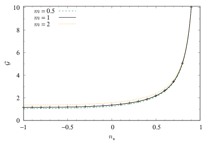
Figure 2: The functional behavior $\mathcal{G}(n_{\star},m)$ of the energy bound (32) in the massive case for various values of $m=0.5,1,2$. The points (pluses) for every $n_{\star}\in\mathbb{Z}/10$, correspond to numerical solutions in later sections (for $m=1$).

Evaluating now the target space integrals for the function $f$ of eq. (20) and the potential $V$ of eq. (24), we get

$$E \geq 12\pi^{2}|B|\mathcal{G}(n_{\star},m),$$

$$\mathcal{G}(n_{\star},m) =\mathcal{F}(n_{\star})\left(\sqrt{\widehat{\alpha}}+\frac{2}{3\sqrt{a}}(1-\widehat{\alpha})^{3/4}\right),$$

$$a =\frac{225\pi^{3}\mathcal{F}^{2}(n_{\star})}{4096m\Gamma^{4}\left(\tfrac{3}{4}\right)}\simeq 0.755\frac{\mathcal{F}^{2}(n_{\star})}{m},$$ (32)

where $\Gamma$ is Euler’s gamma function and $\widehat{\alpha}$ is given by eq. (29). The function $\mathcal{G}(n_{\star},m)$ is shown in fig. 2.

It will again be convenient to define an energy functional, that is divided by the energy bound

$$\epsilon_{B}\equiv\frac{E}{12\pi^{2}|B|\mathcal{G}(n_{\star},m)},$$ (33)

which holds for the massive near-BPS dielectric Skyrme model.

2.4 Equations of motion

The full equations of motion, which are partial differential equations (PDEs), read

$$f^{2}(n_{0})\partial^{2}n_{a}+2f(n_{0})f^{\prime}(n_{0})\partial_{\mu}n_{0}\partial^{\mu}n_{a}+(\partial_{\nu}{\mathbf{n}}\cdot\partial^{\nu}{\mathbf{n}})\partial^{2}n_{a}+(\partial_{\mu}\partial_{\nu}{\mathbf{n}}\cdot\partial^{\nu}{\mathbf{n}})\partial^{\mu}n_{a}$$

$$-(\partial^{2}{\mathbf{n}}\cdot\partial_{\mu}{\mathbf{n}})\partial^{\mu}n_{a}-(\partial_{\mu}{\mathbf{n}}\cdot\partial_{\nu}{\mathbf{n}})\partial^{\mu}\partial^{\nu}n_{a}-f(n_{0})f^{\prime}(n_{0})(\partial_{\mu}{\mathbf{n}}\cdot\partial^{\mu}{\mathbf{n}})\delta_{a0}+m^{2}\delta_{a0} =0,$$ (34)

where $\delta_{ab}$ is Kronecker’s delta and vanishes unless $a=b$. $n_{\star}$ must be strictly smaller than 1 (in the near-BPS case) and therefore $f(n_{0})$ is positive definite and greater than or equal to 1, whereas its derivative $f^{\prime}(n_{0})$ is negative definite for $n_{0}<n_{\star}$ and zero otherwise. Since we work with the mostly positive metric signature, the kinetic term $\partial_{\mu}{\mathbf{n}}\cdot\partial^{\mu}{\mathbf{n}}$ reduces to $|\partial_{i}{\mathbf{n}}|^{2}$ in the static limit, which is positive semi-definite. Therefore, we can see that the effect of a nonconstant $f(n_{0})$ is to increase the kinetic term in the equation of motion (the first term in the above equation) and increase the effective mass term, inside the soliton (i.e. where $n_{0}<n_{\star}$).

For the 1-Skyrmion, we can utilize the hedgehog Ansatz (10) for which the equations of motion reduce to

$$f^{2}\left(\xi_{rr}+\frac{2}{r}\xi_{r}-\frac{1}{r^{2}}\sin 2\xi\right)-ff_{n_{0}}\left(\sin(\xi)\xi_{r}^{2}-\frac{2}{r^{2}}\sin^{3}\xi\right)+\frac{2}{r^{2}}\sin^{2}(\xi)\xi_{rr}$$

$$\mathop{+}\frac{1}{r^{2}}\sin(2\xi)\xi_{r}^{2}-\frac{1}{r^{4}}\sin^{2}(\xi)\sin(2\xi)-m^{2}\sin\xi =0,$$ (35)

with $f=f(n_{0})=f(\cos\xi)$, $f_{n_{0}}=f^{\prime}(n_{0})=f^{\prime}(\cos\xi)$ and we have switched to PDE notation with $\xi_{r}\equiv\frac{\partial\xi}{\partial r}$ and so on.

2.5 Inter-Skyrmion forces

In order to find the forces between two well separated Skyrmions in the model at hand, we follow the analysis of Schroers Schroers:1993yk , adapted to include the pion mass, as in ref. Gudnason:2020arj . The first step is to linearize the ODE (35) for the 1-Skyrmion:

$$f^{2}|\left(\xi_{rr}+\frac{2}{r}\xi_{r}-\frac{2\xi}{r^{2}}\right)-m^{2}\xi=0,$$ (36)

where $f^{2}|$ denotes the limit

$$f^{2}|:=\lim_{\xi\to 0}f^{2}(\cos\xi)=\begin{cases}0,&n_{\star}=1,\\ 1,&n_{\star}<1.\end{cases}$$ (37)

Since we have excluded the BPS limit, we have $n_{\star}<1$ and thus $f^{2}|=1$. The solution to the linearized EOM for the 1-Skyrmion (36) is thus given by

$$\xi=\frac{qm}{4\pi}k_{1}(mr),$$ (38)

where $q$ is a positive constant, $4\pi/m$ is a convenient normalization and $k_{n}$ is the spherical modified Bessel function of the second kind, which has the asymptotic behavior

$$\xi=-q\frac{\mathrm{d}}{\mathrm{d}r}\left(\frac{e^{-mr}}{4\pi mr}\right),$$ (39)

where we have used a recursion relation between the Bessel functions and that $k_{0}(x)=e^{-x}/x$. It is now elementary to show that the linearized Skyrme field at asymptotic distances is given by three orthogonal dipoles

$$U=\mathbf{1}_{2}+\mathrm{i}\boldsymbol{\pi}\cdot\boldsymbol{\sigma},\qquad\boldsymbol{\pi}=(\pi_{1},\pi_{2},\pi_{3}),$$ (40)

with

$$\boldsymbol{\pi}=-q\frac{\partial}{\partial{\mathbf{x}}}\left(\frac{e^{-mr}}{4\pi mr}\right),$$ (41)

and the corresponding quadratic static Lagrangian density is given by

$$\mathcal{L}_{\rm quad}=-\partial_{i}\boldsymbol{\pi}\cdot\partial_{i}\boldsymbol{\pi}-m^{2}\boldsymbol{\pi}\cdot\boldsymbol{\pi}.$$ (42)

The solution (41) is, to leading order in $1/r$, the solution to the equation of motion for the quadratic Lagrangian (42) with a point source of charge $q$

$$(\partial_{i}^{2}-m^{2})\boldsymbol{\pi}=-q\delta^{(3)}({\mathbf{x}}),$$ (43)

whose exact solution is

$$\boldsymbol{\pi}=-\frac{q}{4\pi mr}\frac{\partial}{\partial{\mathbf{x}}}e^{-mr}.$$ (44)

Placing two Skyrmions at ${\mathbf{X}}^{(1),(2)}$ with orientation $\mathscr{R}_{ab}^{(1),(2)}$, where the latter are SO(3) rotation matrices, we have

$$\pi_{a}^{(1)}=-q\mathscr{R}_{ab}^{(1)}\frac{\partial}{\partial x^{b}}\left(\frac{e^{-m|{\mathbf{x}}-{\mathbf{X}}^{(1)}|}}{4\pi m|{\mathbf{x}}-{\mathbf{X}}^{(1)}|}\right),\qquad\pi_{a}^{(2)}=-q\mathscr{R}_{ab}^{(2)}\frac{\partial}{\partial x^{b}}\left(\frac{e^{-m|{\mathbf{x}}-{\mathbf{X}}^{(2)}|}}{4\pi m|{\mathbf{x}}-{\mathbf{X}}^{(2)}|}\right).$$ (45)

The interaction potential can straightforwardly be calculated following refs. Schroers:1993yk ; Gudnason:2020arj , yielding

$$V_{\rm int}\simeq\frac{q^{2}e^{-mR}}{16\pi R}\widehat{{\mathbf{R}}}\cdot\mathscr{O}\widehat{{\mathbf{R}}},$$ (46)

where we have defined ${\mathbf{R}}\equiv|{\mathbf{X}}^{(1)}-{\mathbf{X}}^{(2)}|$, $R\equiv|{\mathbf{R}}|$, $\mathscr{O}\equiv(\mathscr{R}^{(1)})^{\rm T}\mathscr{R}^{(2)}$, and $\widehat{{\mathbf{R}}}\equiv{\mathbf{R}}/R$.

The interaction potential (46), which is valid for $n_{\star}<1$, shows that two Skyrmions at a separation distance $R$ in the same orientation, are mutually repulsive, whereas two Skyrmions in the opposite orientation, are mutually attractive. By opposite orientation, we mean that $\widehat{{\mathbf{R}}}\cdot\mathscr{O}\widehat{{\mathbf{R}}}<0$, which can be obtained by rotating the second Skyrmion by 180 degrees about an axis perpendicular to the axis joining their centers.

To summarize, we have thus shown that for $n_{\star}=1$, the kinetic term is turned off at asymptotic distances, and hence only the Skyrme term and the mass term remain. Since the kinetic term is the origin of the fact that the Skyrmion can be viewed from afar as three orthogonal dipoles, they are the reason for the attraction between the Skyrmions at asymptotic distances (if they are rotated into the attractive channel, see the previous paragraph). To linear order, the Skyrme term does not play a role and hence we have not explicitly shown that the Skyrmions become repulsive in the BPS limit (i.e. $n_{\star}=1$). But since that limit is unphysical, we will not consider such investigation here.

3 Numerical results

In this section we will solve the equations of motion (34) numerically. The method we will use is based on a fourth-order finite-difference scheme with a 5-point stencil for the field derivatives and as the algorithm to find the minimizer of the energy functional from given initial data, we will use the arrested Newton flow described in ref. Gudnason:2020arj . The lattices used in this paper are cubic lattices with $120^{3}$–$240^{3}$ lattice points and lattice spacing $h_{x}\leq 0.15$. The estimated numerical error is less than $10^{-6}$.

As initial data, we will use the rational map approximations (RMA) of ref. Houghton:1997kg for the Skyrmions with topological degrees 1 through 8. The $B=8$ solution obtained from the RMA has dihedral symmetry and we shall denote it as the $B=8_{h}$ solution. We will use two further initial conditions for the $B=8$ sector, which are composed by two $B=4$ cubes placed in the vicinity of one another: one that is a translated copy of the first, which we shall call the $B=8_{u}$ for the untwisted chain and the other is the twisted chain, $B=8_{t}$, obtained by rotating one of the two cubes by 90 degrees about the axis joining their centers. The initial condition for the two cubes is prepared by means of the asymmetric product Ansatz

$$U_{8}=U_{4}U_{4}^{\prime},$$ (47)

with $U_{4}$ one cube made by the RMA for the $B=4$ Skyrmion, translated by a bit more than half the cube’s size in the $-x$ direction and the other cube, $U_{4}^{\prime}$, is translated by the same distance in the $+x$ direction.

A comment in store is about the cusp, present in the function $f$ of eq. (20). That is, the function $f$ is not smooth (as its derivative jumps from a negative value to zero at $n_{0}=n_{\star}$) and a smooth interpolation should be invented. Then the lattice spacing of the numerical lattice should be small enough to resolve the invented smooth interpolation. However, since this is an arbitrariness in the near-BPS version of the model, we chose to deal with this issue very pragmatically, namely to let the discrete derivatives smooth out the cusp. To make sure that it is done consistently in all solutions, we have used the same lattice spacing for all solutions of a given $n_{\star}$.

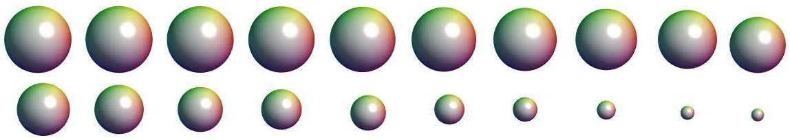
(a) $B=1$

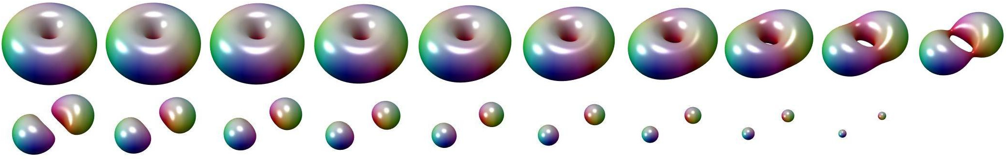
(b) $B=2$

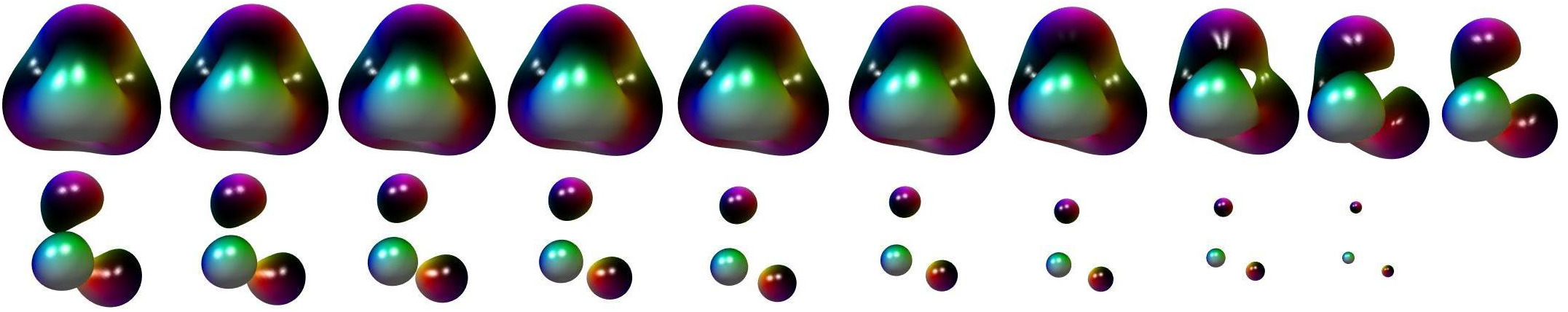
(c) $B=3$

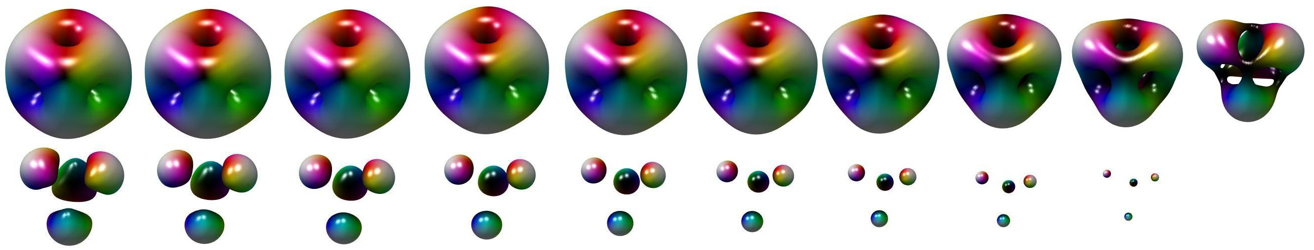
(d) $B=4$

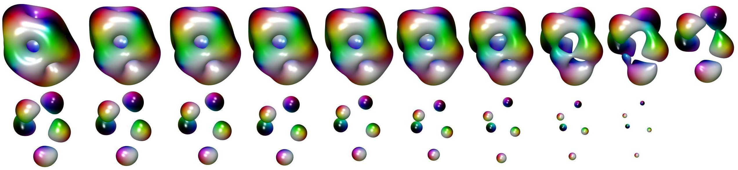
(e) $B=5$

Figure 3: Skyrmion solutions for (a) $B=1$ to (e) $B=5$. Each panel shows 19 figures, except for (a) which shows 20 figures, which are isosurfaces of the topological charge density (TCD) at a quarter of its maximum value, and the first row (from left to right) represents the solution with $n_{\star}$ increasing from $-1$ to $-0.1$ in steps of $0.1$ and in the second row $n_{\star}$ increases from $0$ to $0.8$ (and $0.9$ in panel (a)), again in steps of $0.1$. The color scheme is described in the text.

We are now ready to present the numerical solutions for the near-BPS dielectric Skyrme model for various values of $n_{\star}$, starting with the potential turned off ($m=0$). In this massless version of the model, it is clear that $n_{\star}$ interpolates between the standard massless Skyrme model and a BPS theory. Furthermore, as mentioned above, the BPS theory does not possess multi-Skyrmions – they are unbound. This means that, even though we exclude the point $n_{\star}=1$, we should be able to reach arbitrarily small binding energies by cranking up $n_{\star}$. The question is what happens to the multi-Skyrmions, which we shall now answer with figs. 3 and 5. The figures show arrays of solutions in the form of isosurfaces of the topological charge density (TCD) at a fixed level set, which is taken to be a quarter of the maximum TCD of the given solution. We furthermore color in the isosurface using a standard coloring scheme based on the normalized pion 3-vector

$$\hat{\boldsymbol{\pi}}=\frac{(n_{1},n_{2},n_{3})}{\sqrt{n_{1}^{2}+n_{2}^{2}+n_{3}^{2}}},$$ (48)

such that $\hat{\pi}_{3}=1$ is white, $\hat{\pi}_{3}=-1$ is black and $\hat{\pi}_{3}=0$ is a color determined by $\hat{\pi}_{1}+\mathrm{i}\hat{\pi}_{2}=e^{\mathrm{i}H}$, where $H$ is the hue of the color. In particular $H=0$ is red, $H=2\pi/3$ is green and $H=4\pi/3$ is blue. Each panel in the figures presenting Skyrmion solutions by isosurfaces of their TCD are made of 19 (20) figures, with the first row showing $n_{\star}=-1,-0.9,\ldots,-0.1$ and the second row showing $n_{\star}=0,0.1,\ldots,0.8$ for baryon numbers $B\geq 2$ ($n_{\star}=0,0.1,\ldots,0.9$ for $B=1$).

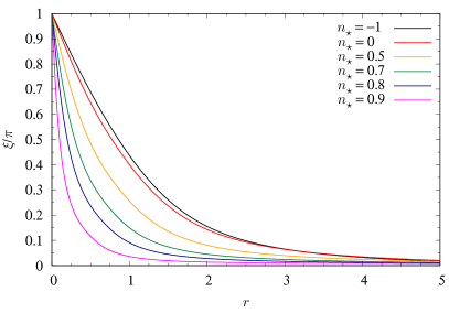
(a) $m=0$

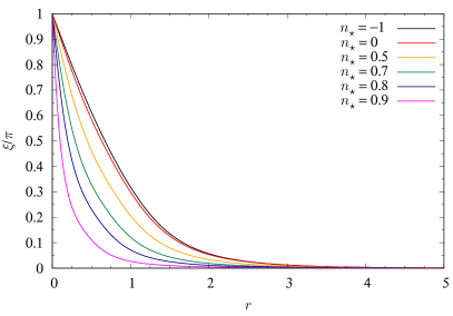
(b) $m=1$

Figure 4: $B=1$ Skyrmion solutions to the ODE (35), for various values of $n_{\star}=-1,0,0.5,0.7,0.8,0.9$.

The 1-Skyrmion retains its spherical symmetry for all values of $n_{\star}$, see fig. 3(a). Although we have divided $f$ by $1-n_{\star}$, the Skyrmions still shrink for $n_{\star}\geq 0$ (if we had not divided by $1-n_{\star}$, $f$ would become very large for $n_{\star}$ approaching 1). Instead now, the tail of the Skyrmion can be captured with the same size lattices, but the BPS nature of the solutions, make them quite peaked at the origin, see fig. 4. For that reason, we have gradually shrunk the lattice spacing for large $n_{\star}$, but not so much that the tails of the solutions would not be contained. In all solutions, the topological charge calculated from the TCD is accurate to the $10^{-4}$ level or better.

As already mentioned, the massless near-BPS dielectric Skyrme model is exactly the standard massless Skyrme model for $n_{\star}=-1$ and thus the solutions coincide in that limit. The 2-Skyrmion is shown in fig. 3(b) and starts out with a torus shape (top left) and is gradually transformed into two separate 1-Skyrmions as $n_{\star}$ tends to 0 (top row). $n_{\star}=0$ is the Skyrmion shown in the left bottom of panel (b). As $n_{\star}$ is further increased to $0.8$ the two 1-Skyrmions become smaller and mutually less interacting. The weak interaction between the two 1-Skyrmions by means of just a mere overlap of their respective soliton tails is the reason for the small binding energy.

Let us summarize the solutions of the remaining three topological sectors in fig. 3. The 3-Skyrmion starts with tetrahedral symmetry for $n_{\star}=-1$ and deforms into three 1-Skyrmions placed at the vertices of a triangle. The 4-Skyrmion starts off with octahedral (cubic) symmetry as a platonic solid for $n_{\star}=-1$ and deforms into a tetrahedrally symmetric soliton for $n_{\star}\simeq-0.2$ and then gradually dissolves into four 1-Skyrmions placed at the vertices of a tetrahedron. The 5-Skyrmion begins with dihedral symmetry and gradually deforms into five 1-Skyrmions placed approximately on the vertices of a face-centered cubic (FCC) lattice with four of them at the vertices of a tetrahedron and the last one a satellite.

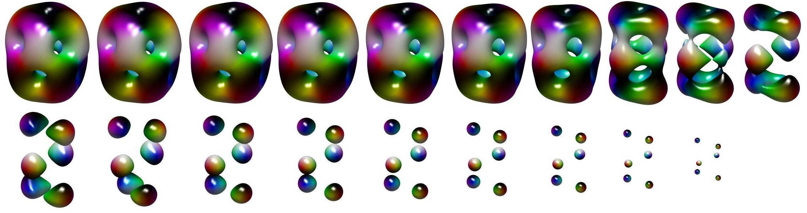
(a) $B=6$

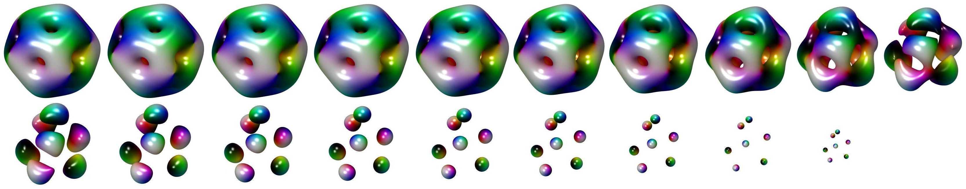
(b) $B=7$

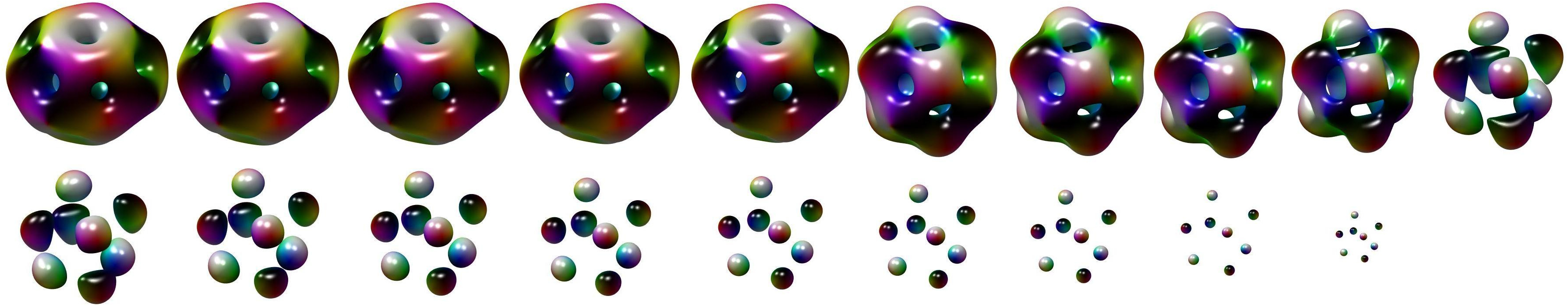
(c) $B=8_{h}$

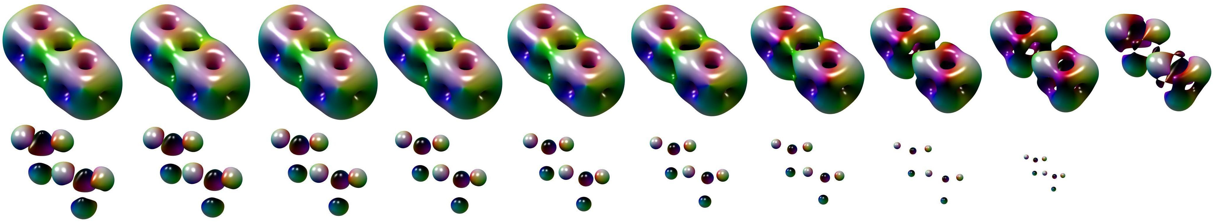
(d) $B=8_{u}$

Figure 5: Skyrmion solutions for (a) $B=1$ to (e) $B=5$. Each panel shows 19 figures, which are isosurfaces of the TCD at a quarter of its maximum value, and the first row (from left to right) represents the solution with $n_{\star}$ increasing from $-1$ to $-0.1$ in steps of $0.1$ and in the second row $n_{\star}$ increases from $0$ to $0.8$, again in steps of $0.1$. The color scheme is described in the text.

Before discussing the emerged pattern, let us summarize also the Skyrmion solutions in the topological charge sectors $B=6$ through $B=8$, shown in fig. 5. For $n_{\star}=-1$ the 6-Skyrmion has dihedral symmetry (fig. 5(a)), the 7-Skyrmion has icosahedral symmetry (fig. 5(b)), the $B=8_{h}$ has dihedral symmetry (fig. 5(c)) and the $B=8_{u}$ has cubic symmetry (fig. 5(d)) Battye:2006na ; Gudnason:2018ysx . Of the two $B=8$ Skyrmion solutions, the $B=8_{h}$ solution with dihedral symmetry has the lowest energy in the standard massless Skyrme model and this is indeed the prediction of the RMA Battye:1997qq . Upon increasing $n_{\star}$ they all deform into $B$ 1-Skyrmions placed at vertices of an FCC-lattice.

A clear pattern has thus emerged and in the near-BPS limit (i.e. $n_{\star}$ tending towards 1), the Skyrmions become point-particle Skyrmions placed at the vertices of an FCC-lattice. This is exactly the kind of solution also possessed by the lightly bound Skyrme model Gillard:2015eia ; Gillard:2016esy , which is simply the standard (massive) Skyrme model with the addition of the potential

$$m_{4}^{2}(1-n_{0})^{4}.$$ (49)

The same type of solution also exists for the loosely bound Skyrme model, with the above potential replaced by

$$m_{2}^{2}(1-n_{0})^{2},$$ (50)

see refs. Gudnason:2016mms ; Gudnason:2016cdo ; Gudnason:2018jia . Furthermore, in the context of holographic QCD or specifically the Sakai-Sugimoto model, the point-particle Skyrmion solutions appear at low energies as a dimensional reduction of point-particle instantons (i.e. instantons with small size moduli) in the limit of large ’t Hooft coupling Baldino:2017mqq .

Before considering the energies of the Skyrmion solutions, we will include the case of the massive near-BPS dielectric Skyrme model, viz. turning on $m=1$ and recalculate the solutions. Because the solutions are quite similar and the deformation to point-particle solutions as 1-Skyrmions placed at the vertices of an FCC-lattice is qualitatively the same, we will not show the analogues of figs. 3 and 5 for $m=1$.

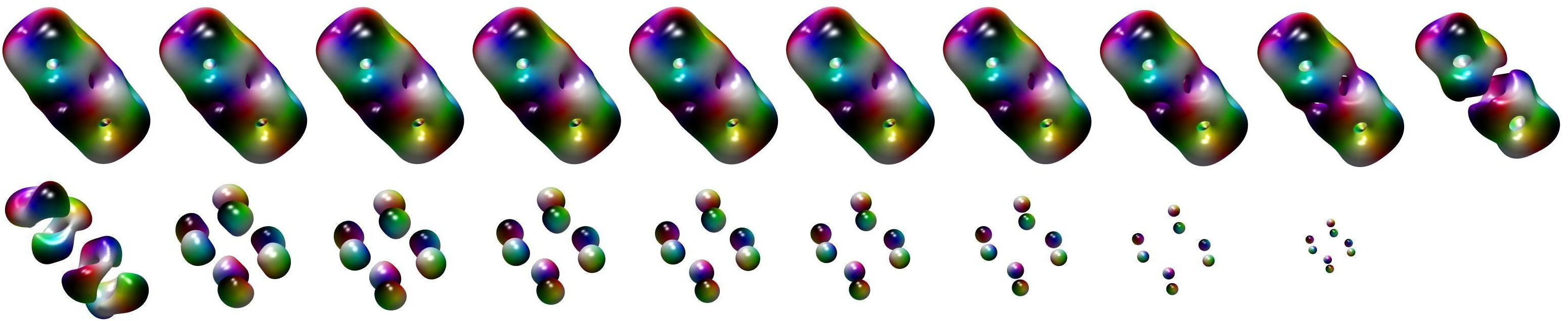
(a) $B=8_{t}$

Figure 6: Skyrmion solutions for the $B=8_{t}$ twisted chain Skyrmion. Each panel shows 19 figures, which are isosurfaces of the TCD at a quarter of its maximum value, and the first row (from left to right) represents the solution with $n_{\star}$ increasing from $-1$ to $-0.1$ in steps of $0.1$ and in the second row $n_{\star}$ increases from $0$ to $0.8$, again in steps of $0.1$. The color scheme is described in the text.

One qualitative difference does manifest itself already for the standard Skyrme model (i.e. at $n_{\star}=-1$). That is, the dihedrally symmetric $B=8_{h}$ Skyrmion is slightly lifted in energy and in particular a twisted chain, $B=8_{t}$, made of two $B=4$ cubes appears as a solution, see fig. 6. The twisted chain, $B=8_{t}$, is obtained from the untwisted chain, $B=8_{u}$ by rotating one of the cubes by 90 degrees about the axis joining their centers. The twisted chain, $B=8_{t}$, does not exist in the massless case ($m=0$), whereas it does exist in the massive case ($m=1$) Battye:2006na . Attempting to find the twisted chain ($B=8_{t}$) in the massless case, results in a relatively fast decay into the dihedrally symmetric solution ($B=8_{h}$), which can be pictured by inflating the middle of the chained solution.

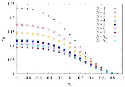
(a) $m=0$

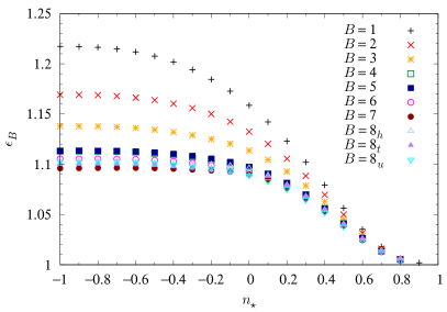
(b) $m=1$

Figure 7: Energy of all stable Skyrmion solutions normalized by their respective energy bounds, $\epsilon_{B}$: (a) eq. (23): without the pion mass term, (b) eq. (33): with the pion mass term and $m=1$.

In fig. 7 we show the energies normalized by their energy bound, $\epsilon_{B}$, of all stable Skyrmion solutions for $B=1$ through $B=8$, with and without the mass term turned on. For the massless case ($m=0$), the energy normalized by its Bogomol’nyi bound is given by eq. (23), whereas in the massive case ($m=1$), it is given by eq. (33). First of all, we can see that all energies lie above their respective energy bound, i.e. $\epsilon_{B}>1$ for all calculated solutions. Since the energies come really close to the bound for $n_{\star}=0.8$, this is a signal of our accuracy being quite good. We do not trust solutions for $n_{\star}>0.8$, because the 1-Skyrmions become too peaked – but at the same time still possessing quite long tails – to be captured reasonably on the lattices, with the lattice spacings used in this paper. Second of all, we can also see by inspection of the figure, that all solutions have positive binding energies.

We should explain what we mean by stable Skyrmions solutions. For $n_{\star}=-1$, the Skyrmions are quite symmetric, possessing a discrete symmetry. It turns out that by increasing $n_{\star}$, such symmetry is broken and the solution gradually transforms into a less symmetric state. Nevertheless, as we shall see shortly, the highly symmetric solution with the symmetries of the $n_{\star}=-1$ solution, continues to exist as a metastable (or perhaps unstable) solution for higher $n_{\star}$. In that sense, only the stable solutions are shown in fig. 7, with the exception of the $B=8$ sector, which is more complicated, see below.

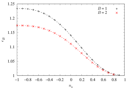
(a)

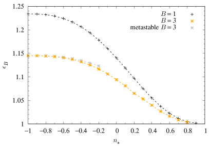
(b)

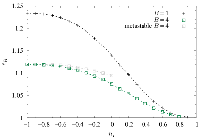
(c)

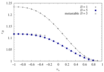
(d)

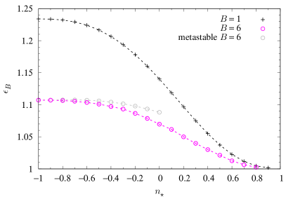
(e)

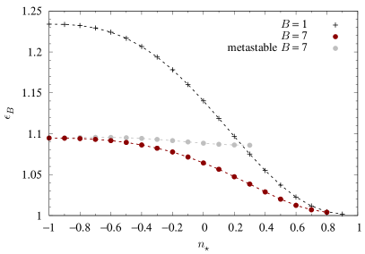
(f)

Figure 8: Energy of all massless Skyrmion solutions, including metastable states (gray lines), normalized by their respective Bogomol’nyi bounds, $\epsilon_{B}$ of eq. (23): for baryon number (a) $B=2$ to (f) $B=7$. For comparison, the normalized energies of the $B=1$ Skyrmion are shown as well.

Fig. 8 shows the energies, topological sector by topological sector, comparing the normalized energy $\epsilon_{B}$ of the $B$-Skyrmion with the 1-Skyrmion, for $B=2$ through $B=7$. With the exception of $B=2$, all the $B$-Skyrmions possess a branch of metastable solutions which look exactly like the $n_{\star}=-1$ solution (up to a slight change in length scale). We might say that the higher the discrete symmetry is, the longer up in $n_{\star}$ the metastable branch of solutions exists; see $B=4,6,7$ in fig. 8(c),(e),(f). The metastable branch for $B=7$ is particularly long lived, so long that it even crosses the energy curve of the 1-Skyrmion: this means that energy could be gained at that point, by splitting the solution up to seven well-separated 1-Skyrmions. This energy, as we will discuss shortly, is called (minus) the binding energy.

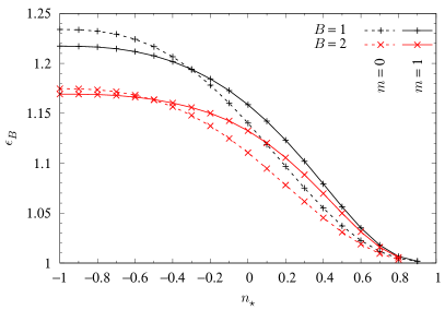
(a)

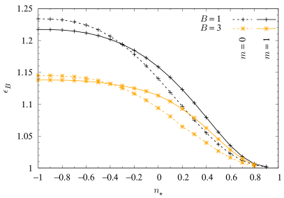
(b)

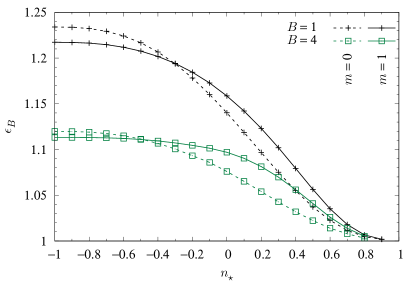
(c)

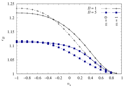
(d)

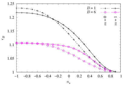
(e)

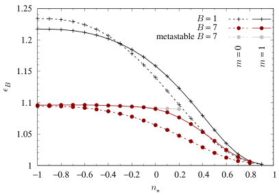
(f)

Figure 9: Energy of all massive Skyrmion solutions, including metastable states (gray lines), normalized by their respective Bogomol’nyi bounds, $\epsilon_{B}$ of eq. (33): for baryon number (a) $B=2$ to (f) $B=7$. For comparison, the normalized energies of the massless $B$-Skyrmions and the massive 1-Skyrmion are shown as well.

We will now turn to the massive case ($m=1$), for which the normalized energies (33) are shown in fig. 9 with solid lines, for topological charges $B=2$ through $B=7$. For comparison with the massless case ($m=0$), we have kept the energies of the stable solutions in each figure, shown with dashed lines. In every figure, the massive and the massless solutions are also compared with the $B=1$ energies. The difference on the $y$-axis between the normalized $B$-Skyrmion energy and the normalized 1-Skyrmion energy, is exactly the binding energy per baryon (nucleon). Hence, as long as the normalized $B$-Skyrmion energy is below the normalized 1-Skyrmion energy, the $B$-Skyrmion is bound and thus at least cannot break up into 1-Skyrmions without an additional kick (external energy). Thus, all the solutions in the entire fig. 9 are bound. In fig. 9, we also show the metastable solutions with gray solid lines, but in contrast to the massless case, there are no metastable branches, except for the $B=7$ solution, see fig. 9(f).

A comment in store is about the absolute (unnormalized) energies of the massive Skyrmion solutions. That is, although it seems that all the massive solutions have smaller energies at $n_{\star}=-1$ than the corresponding massless solutions; that is an artifact of the different normalizations: the massless energies are normalized according to eq. (23), whereas the massive energies are normalized according to eq. (33). In reality, the massive Skyrmion solutions are always heavier in Skyrme units than the corresponding massless solutions, but it turns out that for $B<7$ they are closer to their respective energy bound than the massless ones.

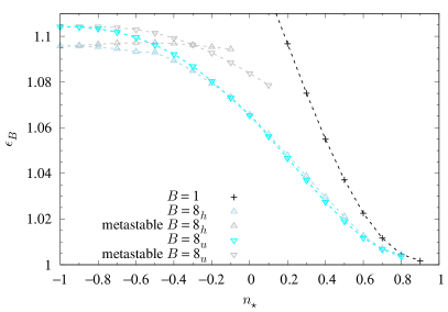
(a) $m=0$

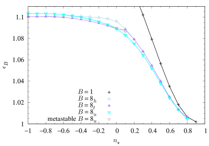
(b) $m=1$

Figure 10: Energy of all Skyrmion solutions normalized by their respective Bogomol’nyi bounds, $\epsilon_{B}$ for $B=8$: (a) eq. (23): without the pion mass term, (b) eq. (33): with the pion mass term and $m=1$.

We now come to the $B=8$ sector, which is the most complicated topological sector that we study in this paper, simply because there are more than one classical (metastable) solution. Fig. 10 shows the $B=8$ sector for both the massless case (fig. 10(a)) and the massive case (fig. 10(b)). Although we have kept the normalized energies of the $B=1$ Skyrmion, we have zoomed the figure so as to better display the features of the $B=8$ energies.

Starting with the massless case $(m=0)$ in fig. 10(a), we have two solutions with different symmetries and hence different shapes, which we shall refer to as the $B=8_{h}$ for the dihedrally symmetric Skyrmion depicted in fig. 5(c) as well as the $B=8_{u}$ denoting the untwisted chain with cubic symmetry, depicted in fig. 5(d). Both of them have metastable branches of solutions, where they retain the discrete symmetry present for $n_{\star}=-1$, which are dihedral and cubic symmetry for the $B=8_{h}$ and $B=8_{u}$, respectively. For $n_{\star}=-1$, which is the standard massless Skyrme model, the stable Skyrmion in the $B=8$ sector is the $B=8_{h}$ dihedrally symmetric one, with $\epsilon_{B}=1.0958$ compared to $\epsilon_{B}=1.1043$ for the $B=8_{u}$ – and so ($B=8_{h}$) is very clearly the stable solution. An interesting twist happens when increasing $n_{\star}$, which is that the $B=8_{u}$ untwisted chain Skyrmion becomes the stable solution for large $n_{\star}$ and the crossover point is around $n_{\star}\sim-0.1$. For $n_{\star}\gtrsim 0.6$, the difference in energy between the two solutions becomes quite small though.

Turning now to the massive case ($m=1$), we have three solutions: the dihedrally symmetric $B=8_{h}$, the twisted chain $B=8_{t}$, with cubic symmetry and the untwisted chain $B=8_{u}$, also with cubic symmetry, see figs. 5(c), 6, and 5(d). The stable solution is probably the twisted chain $B=8_{t}$, in accord with the findings of ref. Battye:2006na , but as stated in the latter reference, the difference in energy between the twisted chain ($B=8_{t}$) and the dihedrally symmetric ($B=8_{h}$) Skyrmion is so small (for $m=1$) that it is beyond the numerical accuracy to decide which one is truly the global minimizer of the energy – and it would be consistent with our results if they are degenerate. We find that $\epsilon_{B}=1.10030$ for the $B=8_{t}$ Skyrmion, compared to $\epsilon_{B}=1.10031$ for the $B=8_{h}$ Skyrmion. The almost degenerate-in-energy solutions $B=8_{t}$ and $B=8_{h}$ are clearly lower in energy with respect to the $B=8_{u}$ solution, see fig. 10(b).

Upon increasing $n_{\star}$ from $n_{\star}=-1$, the twisted chain ($B=8_{t}$) remains the stable solution (and more convincingly so), until $n_{\star}=0$, where the untwisted chain crosses over and becomes the stable solution throughout the range up to $n_{\star}=0.8$ (the maximum of $n_{\star}$ in our calculations). Around the point $n_{\star}=0$, what happens is that the 1-Skyrmions become localized and the model is turned into a point-particle model of Skyrmions. Interestingly, the dihedrally symmetric $B=8_{h}$ solution, initially increases in energy with $n_{\star}$ increasing from $n_{\star}=-1$, then crosses over the previously highest-in-energy $B=8_{u}$ solution at $n_{\star}\sim-0.5$ to become the least stable solution. However, from $n_{\star}\geq 0.1$, the $B=8_{h}$ and $B=8_{t}$ solution fall into an identical pattern of point-particle Skyrmions sitting at the vertices of an FCC lattice, which is reminiscent of the dihedrally symmetric Skyrmion solution. The untwisted chain, $B=8_{u}$, on the other hand, upon dissolving into point-particle Skyrmions, falls into a pattern of two weakly interacting tetrahedrally arranged $B=4$ Skyrmions, which is a different pattern of eight point particles placed at the vertices of an FCC lattice, but with lower energy.

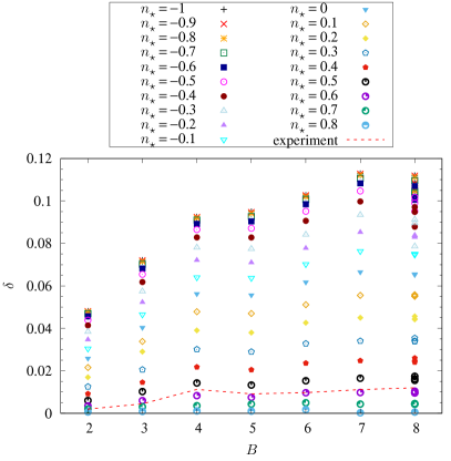
(a) $m=0$

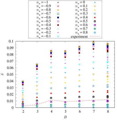
(b) $m=1$

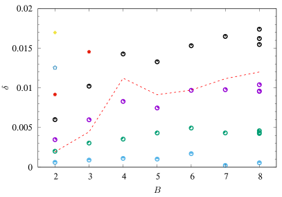
(c) $m=0$

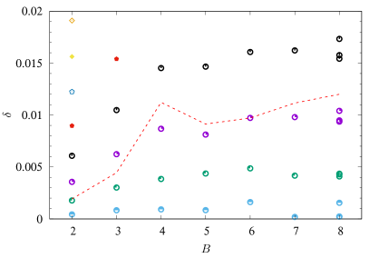
(d) $m=1$

Figure 11: Relative binding energies, $\delta$, of all Skyrmion solutions (a) in the massless case ($m=0$) and (b) in the massive case ($m=1$). The panels (c) and (d) display zoom-ins of the low-binding energy part of the panels (a) and (b), respectively.

We are now finally ready to discuss the relative binding energies, defined by

$$\delta=\frac{BE_{1}-E_{B}}{BE_{1}}=1-\frac{E_{B}}{BE_{1}},$$ (51)

which is a dimensionless quantity and independent of units or normalization of the energies in question.

The relative binding energies, $\delta$ of eq. (51), are displayed in fig. 11 for all the Skyrmion solutions in the near-BPS dielectric Skyrme model. The massless solutions are shown in fig. 11(a) and the massive solutions in fig. 11(b). For the massless case, $\delta$ ranges from about 11.5% down very close to zero, whereas in the massive case it ranges from about 10% again down very close to zero. For small values of $n_{\star}$ – which correspond to the almost standard Skyrme model, the inclusion of the pion mass thus decreases the binding energies a bit, as known in the literature. For higher values of $n_{\star}$, the binding energies drop quite dramatically and for that reason, we have added two extra panels to the figure, zooming in on the low-binding energy region in figs. 11(c) and 11(d). As a guide we have added a red-dashed line depicting the experimentally observed binding energies for nuclei on all panels in fig. 11. We can see that the closest set of Skyrmion solutions is that corresponding to $n_{\star}=0.6$ and some features of physics can be qualitatively seen from the $n_{\star}=0.6$ data points: For example, the relative binding energy increases for $B=2,3,4$ culminating in the stable $\alpha$ particle, but drops for $B=5$ – which in Nature is unstable. We will discuss the results further in the next section.

4 Discussion

In this paper we have considered a near-BPS version suggested in ref. Adam:2020iye of the dielectric Skyrme model, which is yet another modification – albeit a bit drastic one at that – of the standard Skyrme model, in order to lower the binding energies. After reviewing the model and re-deriving the Bogomol’nyi bound, we specify the choice of BPS breaking in terms of the function $f(n_{0})$. We further include the case of adding the pion mass term to the Lagrangian – although that does not logically guarantee a limit with small binding energies. Finally, we perform a numerical investigation of the Skyrmion solutions in the topological charge sectors $B=1$ through $B=8$, with the initial conditions taken from the rational map approximations and for $B=8$ two additional initial conditions made of $B=4$ cubes. First of all we find that, the near-BPS limit studied in this paper, reduces the solutions to the point-particle Skyrmions obtained in other models in the literature. Finally, we demonstrate that realistic classical binding energies can be obtained in this near-BPS model too.

For obtaining a completely realistic theoretical curve for the relative binding energies, further effects must be taken into account, of course. Crucially, of course, is the quantization of spin and isospin, which is a necessity for talking about fermionic states at all. Furthermore, Coulomb energy and isospin breaking effects must be considered too, if fine details of the curve should be trusted. Such refinements are beyond the scope of this paper though. The punchline is that we have lowered the classical binding energies to below the experimentally measured ones and the remaining problem for using the Skyrme model as a model for nuclear theory lies entirely in developing a suitable quantization scheme.

We would like to comment that the commonly known problems with rigid-body quantization might not be as severe in the point-particle models of Skyrmions. The reason is simply that quantizing the cluster of localized 1-Skyrmions as a rigid rotor physically makes no sense. If the overlaps of the tails of the 1-Skyrmions are sufficiently small, it is conceivable that the quantum correction to the energy due to spin and isospin is closer to $B$ times that of the 1-Skyrmions, as compared to the problem in the standard Skyrme model, where the correction is large for the 1-Skyrmion and almost vanishing for $B>1$. This claim needs further investigation and should be part of the development of a mature quantization scheme.

One might naively think that there are many more effects from nuclear physics that must be incorporated into the Skyrme model, in order to produce a working theoretical precision framework for nuclear theory. For example, 3-body forces are known to be important in conventional nuclear theory for lowering binding energies and among many applications, reproducing the oxygen drip line, see e.g. ref. Otsuka:2010 . An interpretation of this is that a repulsive contribution to the binding energy is coming from the two-pion exchange captured by the 3-body force Otsuka:2010 . In the Skyrme-type models, however, all-body forces are in principle taken into account and such additions of particular effects are not necessary, but are supposed to be already built-in. Other forces, like the spin-orbit force, have also recently been shown to be already accounted for correctly in the Skyrme model Halcrow:2020gbm – in contradistinction with early findings.

Since many Skyrme-type models have now been obtained, successfully lowering the classical binding energies to realistic levels, see refs. Gillard:2015eia ; Gillard:2016esy ; Gudnason:2018jia ; Gudnason:2020arj (including the model in the present paper), the time is perhaps ripe to turn to the development of a suitable quantization scheme for applying (some version of) Skyrme theory to nuclear physics.

Acknowledgments

S. B. G. thanks the organizers of “Various topics in mathematical physics,” for the stimulating online virtual conference environment and Andrzej Wereszczynski for giving a talk that motivated this work. S. B. G. thanks the Outstanding Talent Program of Henan University for partial support. The work of S. B. G. is supported by the National Natural Science Foundation of China (Grants No. 11675223 and No. 12071111).

References

- (1) T. H. R. Skyrme, “A Nonlinear field theory,” Proc. Roy. Soc. Lond. A 260, 127-138 (1961).
- (2) T. H. R. Skyrme, “A Unified Field Theory of Mesons and Baryons,” Nucl. Phys. 31, 556-569 (1962).
- (3) S. Weinberg, “Phenomenological Lagrangians,” Physica A 96, no.1-2, 327-340 (1979).
- (4) E. Witten, “Global Aspects of Current Algebra,” Nucl. Phys. B 223, 422-432 (1983).
- (5) E. Witten, “Current Algebra, Baryons, and Quark Confinement,” Nucl. Phys. B 223, 433-444 (1983).
- (6) G. S. Adkins, C. R. Nappi and E. Witten, “Static Properties of Nucleons in the Skyrme Model,” Nucl. Phys. B 228, 552 (1983).
- (7) I. Zahed and G. E. Brown, “The Skyrme Model,” Phys. Rept. 142, 1-102 (1986).
- (8) R. A. Battye and P. M. Sutcliffe, “Symmetric skyrmions,” Phys. Rev. Lett. 79, 363-366 (1997) [arXiv:hep-th/9702089 [hep-th]].
- (9) D. Harland, “Topological energy bounds for the Skyrme and Faddeev models with massive pions,” Phys. Lett. B 728, 518-523 (2014) [arXiv:1311.2403 [hep-th]].
- (10) C. Adam and A. Wereszczynski, “Topological energy bounds in generalized Skyrme models,” Phys. Rev. D 89, no.6, 065010 (2014) [arXiv:1311.2939 [hep-th]].
- (11) L. D. Faddeev, “Some Comments on the Many Dimensional Solitons,” Lett. Math. Phys. 1, 289 (1976).
- (12) N. S. Manton and P. J. Ruback, “Skyrmions in Flat Space and Curved Space,” Phys. Lett. B 181, 137-140 (1986).
- (13) L. A. Ferreira and W. J. Zakrzewski, “A Skyrme-like model with an exact BPS bound,” JHEP 09, 097 (2013) [arXiv:1307.5856 [hep-th]].
- (14) C. Adam, J. Sanchez-Guillen and A. Wereszczynski, “A Skyrme-type proposal for baryonic matter,” Phys. Lett. B 691, 105-110 (2010) [arXiv:1001.4544 [hep-th]].
- (15) C. Adam, J. Sanchez-Guillen and A. Wereszczynski, “A BPS Skyrme model and baryons at large ,” Phys. Rev. D 82, 085015 (2010) [arXiv:1007.1567 [hep-th]].
- (16) T. Sakai and S. Sugimoto, “Low energy hadron physics in holographic QCD,” Prog. Theor. Phys. 113, 843-882 (2005) [arXiv:hep-th/0412141 [hep-th]].
- (17) L. Bartolini, S. Bolognesi and A. Proto, “From the Sakai-Sugimoto Model to the Generalized Skyrme Model,” Phys. Rev. D 97, no.1, 014024 (2018) [arXiv:1711.03873 [hep-th]].
- (18) J. M. Speight, “Near BPS Skyrmions and Restricted Harmonic Maps,” J. Geom. Phys. 92, 30-45 (2015) [arXiv:1406.0739 [hep-th]].
- (19) S. B. Gudnason, M. Barsanti and S. Bolognesi, “Near-BPS baby Skyrmions,” [arXiv:2006.01726 [hep-th]].
- (20) R. A. Leese, M. Peyrard and W. J. Zakrzewski, “Soliton Scatterings in Some Relativistic Models in (2+1)-dimensions,” Nonlinearity 3, 773-808 (1990).
- (21) B. M. A. G. Piette, W. J. Zakrzewski, H. J. W. Mueller-Kirsten and D. H. Tchrakian, “A Modified Mottola-Wipf model with sphaleron and instanton fields,” Phys. Lett. B 320, 294-298 (1994).
- (22) B. M. A. G. Piette, B. J. Schroers and W. J. Zakrzewski, “Multi - solitons in a two-dimensional Skyrme model,” Z. Phys. C 65, 165-174 (1995) [arXiv:hep-th/9406160 [hep-th]].
- (23) M. Gillard, D. Harland and M. Speight, “Skyrmions with low binding energies,” Nucl. Phys. B 895, 272-287 (2015) [arXiv:1501.05455 [hep-th]].
- (24) S. B. Gudnason, “Loosening up the Skyrme model,” Phys. Rev. D 93, no.6, 065048 (2016) [arXiv:1601.05024 [hep-th]].
- (25) S. B. Gudnason and M. Nitta, “Modifying the pion mass in the loosely bound Skyrme model,” Phys. Rev. D 94, no.6, 065018 (2016) [arXiv:1606.02981 [hep-ph]].
- (26) S. B. Gudnason, B. Zhang and N. Ma, “Generalized Skyrme model with the loosely bound potential,” Phys. Rev. D 94, no.12, 125004 (2016) [arXiv:1609.01591 [hep-ph]].
- (27) S. B. Gudnason, “Exploring the generalized loosely bound Skyrme model,” Phys. Rev. D 98, no.9, 096018 (2018) [arXiv:1805.10898 [hep-ph]].
- (28) M. Gillard, D. Harland, E. Kirk, B. Maybee and M. Speight, “A point particle model of lightly bound skyrmions,” Nucl. Phys. B 917, 286-316 (2017) [arXiv:1612.05481 [hep-th]].
- (29) S. Baldino, S. Bolognesi, S. B. Gudnason and D. Koksal, “Solitonic approach to holographic nuclear physics,” Phys. Rev. D 96, no.3, 034008 (2017) [arXiv:1703.08695 [hep-th]].
- (30) C. Adam, K. Oles and A. Wereszczynski, “The Dielectric Skyrme model,” Phys. Lett. B 807, 135560 (2020) [arXiv:2005.00018 [hep-th]].
- (31) L. A. Ferreira, “Exact self-duality in a modified Skyrme model,” JHEP 07, 039 (2017) [arXiv:1705.01824 [hep-th]].
- (32) C. Adam, L. A. Ferreira, E. da Hora, A. Wereszczynski and W. J. Zakrzewski, “Some aspects of self-duality and generalised BPS theories,” JHEP 08, 062 (2013) [arXiv:1305.7239 [hep-th]].
- (33) L. A. Ferreira and Y. Shnir, “Exact Self-Dual Skyrmions,” Phys. Lett. B 772, 621-627 (2017) [arXiv:1704.04807 [hep-th]].
- (34) C. Naya and K. Oles, “Background fields and self-dual Skyrmions,” Phys. Rev. D 102, no.2, 025007 (2020) [arXiv:2004.07069 [hep-th]].
- (35) D. Tong and K. Wong, “Vortices and Impurities,” JHEP 01, 090 (2014) [arXiv:1309.2644 [hep-th]].
- (36) D. Bazeia, E. da Hora, C. dos Santos and R. Menezes, “Generalized self-dual Chern-Simons vortices,” Phys. Rev. D 81, 125014 (2010) [arXiv:1006.3955 [hep-th]].
- (37) D. Bazeia, E. da Hora, C. dos Santos and R. Menezes, “BPS Solutions to a Generalized Maxwell-Higgs Model,” Eur. Phys. J. C 71, 1833 (2011) [arXiv:1201.2974 [hep-th]].
- (38) D. Bazeia, R. Casana, E. da Hora and R. Menezes, “Generalized self-dual Maxwell-Chern-Simons-Higgs model,” Phys. Rev. D 85, 125028 (2012) [arXiv:1206.0998 [hep-th]].
- (39) P. Sutcliffe, “Skyrmions, instantons and holography,” JHEP 08, 019 (2010) [arXiv:1003.0023 [hep-th]].
- (40) P. Sutcliffe, “Skyrmions in a truncated BPS theory,” JHEP 04, 045 (2011) [arXiv:1101.2402 [hep-th]].
- (41) R. Battye and P. Sutcliffe, “Skyrmions and the pion mass,” Nucl. Phys. B 705, 384-400 (2005) [arXiv:hep-ph/0410157 [hep-ph]].
- (42) R. Battye and P. Sutcliffe, “Skyrmions with massive pions,” Phys. Rev. C 73, 055205 (2006) [arXiv:hep-th/0602220 [hep-th]].
- (43) C. Houghton and S. Magee, “The Effect of pion mass on skyrme configurations,” EPL 77, no.1, 11001 (2007) [arXiv:hep-th/0602227 [hep-th]].
- (44) R. Battye, N. S. Manton and P. Sutcliffe, “Skyrmions and the alpha-particle model of nuclei,” Proc. Roy. Soc. Lond. A 463, 261-279 (2007) [arXiv:hep-th/0605284 [hep-th]].
- (45) R. A. Battye, N. S. Manton, P. M. Sutcliffe and S. W. Wood, “Light Nuclei of Even Mass Number in the Skyrme Model,” Phys. Rev. C 80, 034323 (2009) [arXiv:0905.0099 [nucl-th]].
- (46) P. H. C. Lau and N. S. Manton, “States of Carbon-12 in the Skyrme Model,” Phys. Rev. Lett. 113, no.23, 232503 (2014) [arXiv:1408.6680 [nucl-th]].
- (47) C. J. Halcrow, “Vibrational quantisation of the B = 7 Skyrmion,” Nucl. Phys. B 904, 106-123 (2016) [arXiv:1511.00682 [hep-th]].
- (48) J. I. Rawlinson, “An Alpha Particle Model for Carbon-12,” Nucl. Phys. A 975, 122-135 (2018) [arXiv:1712.05658 [nucl-th]].
- (49) C. J. Halcrow, C. King and N. S. Manton, “A dynamical -cluster model of 16O,” Phys. Rev. C 95, no.3, 031303 (2017) [arXiv:1608.05048 [nucl-th]].
- (50) C. J. Halcrow, C. King and N. S. Manton, “Oxygen-16 Spectrum from Tetrahedral Vibrations and their Rotational Excitations,” Int. J. Mod. Phys. E 28, no.04, 1950026 (2019) [arXiv:1902.09424 [nucl-th]].
- (51) J. I. Rawlinson, “Coriolis terms in Skyrmion Quantization,” Nucl. Phys. B 949, 114800 (2019) [arXiv:1908.03414 [nucl-th]].
- (52) S. B. Gudnason and C. Halcrow, “Vibrational modes of Skyrmions,” Phys. Rev. D 98, no.12, 125010 (2018) [arXiv:1811.00562 [hep-th]].
- (53) G. H. Derrick, “Comments on nonlinear wave equations as models for elementary particles,” J. Math. Phys. 5, 1252-1254 (1964).
- (54) M. Harada and K. Yamawaki, “Hidden local symmetry at loop: A New perspective of composite gauge boson and chiral phase transition,” Phys. Rept. 381, 1-233 (2003) [arXiv:hep-ph/0302103 [hep-ph]].
- (55) L. Marleau, “The Skyrme Model and Higher Order Terms,” Phys. Lett. B 235, 141 (1990).
- (56) L. Marleau, “All orders skyrmions,” Phys. Rev. D 45, 1776-1781 (1992).
- (57) L. Marleau and J. F. Rivard, “A generating function for all orders skyrmions,” Phys. Rev. D 63, 036007 (2001) [arXiv:hep-ph/0011052 [hep-ph]].
- (58) N. Manton and P. Sutcliffe, “Topological Solitons,” Cambridge Monographs on Mathematical Physics, (2004).
- (59) B. J. Schroers, “Dynamics of moving and spinning Skyrmions,” Z. Phys. C 61, 479-494 (1994) [arXiv:hep-ph/9308236 [hep-ph]].
- (60) S. B. Gudnason and J. M. Speight, “Realistic classical binding energies in the -Skyrme model,” JHEP 07, 184 (2020) [arXiv:2004.12862 [hep-th]].
- (61) C. J. Houghton, N. S. Manton and P. M. Sutcliffe, “Rational maps, monopoles and Skyrmions,” Nucl. Phys. B 510, 507-537 (1998) [arXiv:hep-th/9705151 [hep-th]].
- (62) T. Otsuka, T. Suzuki, J. D. Holt, A. Schwenk and Y. Akaishi, “Three-Body Forces and the Limit of Oxygen Isotopes,” Phys. Rev. Lett. 105, 032501 (2010).
- (63) C. Halcrow and D. Harland, “An attractive spin-orbit potential from the Skyrme model,” Phys. Rev. Lett. 125, no.4, 042501 (2020) [arXiv:2007.01304 [hep-th]].