Designing sequence set with minimal peak side-lobe level for applications in high resolution RADAR imaging

Abstract

Constant modulus sequence set with low peak side-lobe level is a necessity for enhancing the performance of modern active sensing systems like Multiple Input Multiple Output (MIMO) RADARs. In this paper, we consider the problem of designing a constant modulus sequence set by minimizing the peak side-lobe level, which can be cast as a non-convex minimax problem, and propose a Majorization-Minimization technique based iterative monotonic algorithm. The iterative steps of our algorithm are computationally not very demanding and they can be efficiently implemented via Fast Fourier Transform (FFT) operations. We also establish the convergence of our proposed algorithm and discuss the computational and space complexities of the algorithm. Finally, through numerical simulations, we illustrate the performance of our method with the state-of-the-art methods. To highlight the potential of our approach, we evaluate the performance of the sequence set designed via our approach in the context of probing sequence set design for MIMO RADAR angle-range imaging application and show results exhibiting good performance of our method when compared with other commonly used sequence set design approaches.

Index Terms– RADAR waveform design, peak side-lobe level, PAPR, active sensing systems, Majorization-Minimization, MIMO RADAR.

I Introduction and literature review

In recent years, Multiple Input Multiple Output (MIMO) RADAR has become a trending technology and plays a key role in modern warfare systems. Unlike the phased array RADAR system [1] which transmits the scaled versions of single sequence, the MIMO RADAR system will take advantage of the waveform diversity [2] and transmits more number of sequences simultaneously which results in creating a very large virtual aperture that inturn gives enhanced resolution images [3] and paves way for better target detection [4, 5, 6, 7]. But to reap all the benefits of the MIMO RADAR, the probing sequence set employed should have good correlation side-lobe levels [8, 9]. In any practical RADAR system, there are many challenges like limited energy budget, high cost of the practical hardware components, and the necessity to work on the linear range of power amplifiers, which force one to consider using either unimodular (or) low Peak to the Average Power Ratio (PAPR) constrained probing set of sequences [10, 11]. Besides MIMO RADAR, some notable applications where constant modulus sequence set with better correlation side-lobe levels play a prominent role are wireless communication systems [9, 10], MIMO SONAR [12, 13, 14, 15], Cryptography [9], channel estimation [11, 16], CDMA and spread spectrum applications [17, 18, 19, 20]. Hence, designing constant modulus sequence set with better auto-correlation and cross-correlation side-lobe levels is always desired.

Designing sequences with good auto-correlation properties for applications in active sensing, wireless communication is an active area of research and countless number of researchers have contributed to it. In the following, we will briefly discuss some key contributions. The foundation for research on the probing signal design is done by notable researchers like Nyquist, Shannon, Tesla, and was continued by the Barker, Golomb, Frank, Woodward, etc. In the early years, researchers studied the single sequence design problem via analytical approaches and proposed the maximal length, Gold, Kasami sequences which are known to possess better periodic correlation properties, and later the binary Barker [21], Golomb [22], Frank [23], polyphase [24] sequences have been developed which have better aperiodic correlation properties. A major drawback of the analytical approaches is the sequences obtained by these approaches are known to exist only for the limited lengths and have lesser degrees of freedom. To overcome such issues, in the recent decade (or) so, researchers have used numerical optimization methods and used different metrics (depending upon the applications) and designed algorithms to generate larger length sequences with good correlation properties. The authors in [25, 26, 27] proposed methods to design sequence with good correlation properties by optimizing the correlation related metrics like Integrated Side-lobe Level (ISL) and approximated Peak Side-lobe level (PSL), works done in [28, 29, 30] studied the sequence design along with correlation and spectral constraints. The authors in [31] studied the problem of designing sequences with better ambiguity function - which ensures sequences with good autocorrelation and as well as immune to Doppler ambiguities. All the above mentioned works studied only the single sequence design problem and in the following, we discuss the literature on the sequence set design which is the main focus of this paper.

The authors in [32] minimized the approximated ISL metric using the alternating minimization method and proposed the Multi-CAN algorithm that can design very large length sequence sets. In [33, 34], the authors have proposed an optimization technique that minimizes the original ISL metric and the resultant algorithm was capable of designing large length sequence sets with better correlation side-lobe levels than the one generated via the Multi-CAN approach. Slightly different from the ISL based approaches, the authors in [35] tried to minimize the PSL metric by approximating it with a Chebyshev metric and designed sequence set for applications in MIMO RADAR. An iterative direct search algorithm that updates each element of the sequence set sequentially while considering the remaining elements fixed using exhaustive pattern search method was proposed in [36]. In [37], the authors considered the Pareto function (weighted combination) of PSL, ISL metrics and optimized using the Block Coordinate Descent (BCD) method and proposed an algorithm BiST to design set of sequences with discrete phase constraint. The authors in [38] optimized the ISL metric via Coordinate Descent (CD) framework to design set of sequences that meets Welch bound on the ISL value. It is very clear from the literature survey, that none of the researchers have designed sequence set by directly minimizing the peak side-lobe level metric - a major reason being the challenging nature of the design metric as it is not differentiable and the associated optimization problem is a saddle point problem. A brief summary of the literature survey on the sequence set design problem is as follows:

• There are analytical as well as computational approaches minimizing the ISL metric to design large length single sequences with better periodic, aperiodic correlation properties.

• To design sequence set, there are ISL minimization based algorithms (Multi-CAN, MM-Corr, ISL-NEW, Iteration Direct Search Algorithm) but none that can generate sequence set by optimizing the exact PSL metric.

• There is PSL (or) ISL (or) both minimization based algorithm named as BiST, which can able to design set of sequences but only under the discrete phase constraint.

So to the best of our knowledge, nobody has approached the problem of designing sequence set by directly minimizing (without any approximation) the peak side-lobe level metric. One may ask, what can one achieve special by minimizing the PSL when compared to the ISL metric? The answer can be explained as follows - In a RADAR system with a matched filter receiver, the peak side-lobe level of the transmit sequence will dictate the false alarm probability, so the lower the PSL level, the lower the probability of false alarm. Thus, on top of the computational challenge, designing sequence set by minimizing the PSL metric has also pratical significance.

The major contributions of this paper are as follows:

• We have developed a monotonic algorithm which is based on the technique of Majorization-Minimization to design a constant modulus sequence set by minimizing the PSL metric.

• We show a computationally efficient way of implementing our proposed algorithm using FFT and IFFT operations.

• We prove the convergence of our algorithm to a stationary point of the PSL metric.

• Finally, we evaluate the performance of the proposed algorithm through numerical simulations for different problem dimensions and compare them with the state-of-the-art techniques. We also evaluate the proposed algorithm in the context of the MIMO RADAR imaging application.

The rest of the paper is organized as follows. Formulation of the sequence set design problem and a review of the Majorization-Minimization technique is discussed in section II. The proposed algorithm, its proof of monotonic convergence to the stationary point, computational and space complexities of the proposed algorithm are discussed in section III. The numerical simulations of the proposed algorithm and the MIMO RADAR angle-range imaging experimental results of the generated sequence set are given in section IV and finally section V concludes the paper.

Throughout the paper the following mathematical notations are used hereafter: Matrices are indicated by the boldface upper case letters, column vectors are indicated by the boldface lowercase letters and the scalars are indicated by the italics. Complex conjugate, conjugate transpose, and the transpose are indicated by the superscripts $()^{*},()^{H},()^{T}$. Trace of a matrix is denoted by $\text{Tr}()$ . $\boldsymbol{z}_{i}(m)$ denote the $m^{th}$ element of a vector $\boldsymbol{\boldsymbol{z}}_{i}$. $\boldsymbol{\boldsymbol{I}}_{w}$ denote the $w\times w$ identity matrix. $\boldsymbol{\boldsymbol{O}}_{w}$ denote the $w\times w$ matrix full of zeros. $||.||_{2}$ denote the $l_{2}$ norm. $\text{vec}(\boldsymbol{\boldsymbol{A}})$ is a column vector stacked with all the columns of matrix-$\boldsymbol{\boldsymbol{A}}$. $\left|.\right|^{2}$ denote the absolute squared value. The maximum eigenvalue of $\boldsymbol{\boldsymbol{\boldsymbol{A}}}$ is denoted by $\lambda_{\text{max}}(\boldsymbol{\boldsymbol{\boldsymbol{A}}})$. $\mathbb{R}$ and $\mathbb{C}$ represent the real and complex fields. The real and imaginary parts are denoted by $\text{Re}(.)$ and $\text{Im}(.)$ respectively. $\nabla g(.)$ (or) $\partial g(.)$ denote the gradient of a function $g(.).$ $\boldsymbol{\boldsymbol{z}}^{t}$ denote the value of $\boldsymbol{\boldsymbol{z}}$ at $t^{th}$ iteration. $\bigodot$ represents the Hadamard product.

II PROBLEM FORMULATION AND MAJORIZATION-MINIMIZATION METHOD

II-A PROBLEM FORMULATION

Let $\left\{\boldsymbol{\boldsymbol{s}}_{1},\boldsymbol{\boldsymbol{s}}_{2},...,\boldsymbol{\boldsymbol{s}}_{L}\right\}$ denote the $L$ number of $M$ length probing phase sequences. The Peak Side-lobe Level (PSL) metric which is our design criterion to evaluate the quality of the sequence-set is defined as:

$$\text{PSL}=\text{\text{$\underset{k\in a_{k}}{\text{\text{max}}}$}}\left\{\Bigl{|}r_{i,j}(k)\Bigr{|}\right\},\,i,j=1,2,..,L,$$ (1)

where

$$a_{k}=\begin{cases}1,2,...,(M-1)&\text{if}\,i=j\\ 0,1,2,..,(M-1)&\text{if}\,i\neq j\end{cases}$$

and $r_{i,j}(k)$ is the aperiodic cross-correlation of the sequences $\boldsymbol{\boldsymbol{s}}_{i},\boldsymbol{\boldsymbol{s}}_{j}$ at lag $k$, which is defined as:

$$r_{i,j}(k)=\sum_{m=1}^{M-k}s_{i}^{*}(m)s_{j}(m+k)=r_{j,i}^{*}(-k)$$ (2)

which will be the auto-correlation function when $i=j$. Since we are interested in sequence set design with each element of any sequence to have constant modulus, the problem of interest can be formulated as:

$$\underset{\left\{\boldsymbol{\boldsymbol{s}}_{1},\boldsymbol{\boldsymbol{s}}_{2},.,\boldsymbol{\boldsymbol{s}}_{L}\right\}}{\text{\text{min}}} \text{$\underset{k\in a_{k}}{\text{\text{max}}}$}\hphantom{nn}\Bigl{|}r_{i,j}(k)\Bigr{|},\,i,j=1,..,L,$$ (3)

subject to $$\bigl{|}\boldsymbol{\boldsymbol{s}}_{i}(m)\bigr{|}=1,\,i=1,..,L;m=1,..,M.$$

The problem in (3) is a minimax problem and is non-convex in nature. Moreover, the objective function (PSL metric) is non-differentiable (due to the maximum), which makes the problem even more challenging. Before we move on to the presentation of our algorithm, we will present a brief summary of the Majorization-Minimization (MM) framework, which would be central in the development of our algorithm.

II-B Majorization-Minimization Method

In this sub-section, we will briefly discuss the general Majorization-Minimization method (which is defined for minimization problems) and its extension to the minimax optimization problems.

II-B1 Majorization-Minimization for minimization problems

Majorization-Minimization (MM) method was first developed by De Leeuw while solving the multidimensional scaling problem [39]. Later, after realizing its strength to solve non-convex (or) even convex problems efficiently, many researchers adopted the technique to address problems in various fields like signal processing, communications, machine learning, etc. Consider a minimization problem as follows:

$$\min_{\boldsymbol{\boldsymbol{x}\in\boldsymbol{\boldsymbol{\boldsymbol{\chi}}}}}f(\boldsymbol{\boldsymbol{x}})$$ (4)

where $f(\boldsymbol{\boldsymbol{x}})$ is some non-linear function and $\boldsymbol{\boldsymbol{\boldsymbol{\chi}}}$ denotes the constraint set. The MM approach is two-step method [40] in which at the first step, at any given point $\boldsymbol{\boldsymbol{\boldsymbol{x}}}^{t}$ ($\boldsymbol{\boldsymbol{\boldsymbol{x}}}$ at $t^{th}$ iteration), an upper bound (majorization) function $u(\boldsymbol{\boldsymbol{\boldsymbol{x}}}|\boldsymbol{\boldsymbol{\boldsymbol{x}}}^{t})$ to the original objective function $f(\boldsymbol{\boldsymbol{x}})$ is constructed, and in the second step the upper bound function $u(\boldsymbol{\boldsymbol{\boldsymbol{x}}}|\boldsymbol{\boldsymbol{\boldsymbol{x}}}^{t})$ is minimized to obtain the next iterate point $\boldsymbol{\boldsymbol{\boldsymbol{x}}}^{t+1}$. Again at $\boldsymbol{\boldsymbol{\boldsymbol{x}}}^{t+1}$, the above mentioned two steps are implemented and the series of these steps will continue until the optimum stationary point of an original function $f(\boldsymbol{\boldsymbol{x}})$ is reached. The majorization function $u(\boldsymbol{\boldsymbol{\boldsymbol{x}}}|\boldsymbol{\boldsymbol{\boldsymbol{x}}}^{t})$ (which is constructed in the first step) has to satisfy the following properties:

$$u(\boldsymbol{\boldsymbol{\boldsymbol{x}}}^{t}|\boldsymbol{\boldsymbol{\boldsymbol{x}}}^{t})=f(\boldsymbol{\boldsymbol{\boldsymbol{x}}}^{t}),\quad\forall\boldsymbol{\boldsymbol{x}}\in\boldsymbol{\boldsymbol{\boldsymbol{\chi}}}.$$ (5)

$$u(\boldsymbol{\boldsymbol{x}}|\boldsymbol{\boldsymbol{\boldsymbol{x}}}^{t})\geq f(\boldsymbol{\boldsymbol{x}}),\quad\forall\boldsymbol{\boldsymbol{x}}\in\boldsymbol{\boldsymbol{\boldsymbol{\chi}}}.$$ (6)

For a given problem, more than one possible majorization function will exist and this gives a possibility to develop two different iterative algorithms for the same problem. A survey to construct the majorizing function is given in [41]. The objective function value evaluated at every iteration generated by MM will satisfy the descent property, i.e.

$$f(\boldsymbol{\boldsymbol{\boldsymbol{x}}}^{t+1})\leq u(\boldsymbol{\boldsymbol{\boldsymbol{x}}}^{t+1}|\boldsymbol{\boldsymbol{\boldsymbol{x}}}^{t})\leq u(\boldsymbol{\boldsymbol{\boldsymbol{x}}}^{t}|\boldsymbol{\boldsymbol{\boldsymbol{x}}}^{t})=f(\boldsymbol{\boldsymbol{\boldsymbol{x}}}^{t}).$$ (7)

II-B2 Majorization-Minimization for minimax problems

Consider the minimax problem as follows:

$$\min_{\boldsymbol{\boldsymbol{y}\in\boldsymbol{\boldsymbol{\boldsymbol{\chi}}}}}g(\boldsymbol{\boldsymbol{y}}),$$ (8)

where $g(\boldsymbol{\boldsymbol{y}})=\underset{k=1,..,N}{\text{max}}g_{k}(\boldsymbol{\boldsymbol{y}})$. Similar to the case of minimization problems, the majorization function for the objective in (8) can be constructed as follows:

$$u(\boldsymbol{\boldsymbol{y}}|\boldsymbol{\boldsymbol{y}}^{t})=\underset{k=1,..,N}{\text{max}}\tilde{u}_{k}(\boldsymbol{\boldsymbol{y}}|\boldsymbol{\boldsymbol{y}}^{t}),$$ (9)

where each $\tilde{u}_{k}(\boldsymbol{\boldsymbol{y}}|\boldsymbol{\boldsymbol{y}}^{t})$ is an upper bound for the respective $g_{k}(\boldsymbol{\boldsymbol{y}})$ at any given $\boldsymbol{\boldsymbol{y}}^{t},\,\forall k$. Here, every majorization function $\tilde{u}_{k}(\boldsymbol{\boldsymbol{y}}|\boldsymbol{\boldsymbol{y}}^{t}),\,\forall k$ will also satisfy the conditions mentioned in (5), (6) i.e.,

$$\tilde{u}_{k}(\boldsymbol{\boldsymbol{y}}^{t}|\boldsymbol{\boldsymbol{y}}^{t})=g_{k}(\boldsymbol{\boldsymbol{y}}^{t}),\,\forall k,\boldsymbol{y}\in\boldsymbol{\boldsymbol{\boldsymbol{\chi}}}$$ (10)

$$\tilde{u}_{k}(\boldsymbol{\boldsymbol{y}}|\boldsymbol{\boldsymbol{y}}^{t})\geq g_{k}(\boldsymbol{\boldsymbol{y}}),\,\forall k,\boldsymbol{y}\in\boldsymbol{\boldsymbol{\boldsymbol{\chi}}}$$ (11)

It can be easily shown that the choice of $u(\boldsymbol{\boldsymbol{y}}|\boldsymbol{\boldsymbol{y}}^{t})$ in (9) is a global upper bound function of $g(\boldsymbol{\boldsymbol{y}})$, i.e.,

$$u(\boldsymbol{\boldsymbol{y}}^{t}|\boldsymbol{\boldsymbol{y}}^{t})=\underset{k=1,..,N}{\text{max}}\tilde{u}_{k}(\boldsymbol{\boldsymbol{y}}^{t}|\boldsymbol{\boldsymbol{y}}^{t})=\underset{k=1,..,N}{\text{max}}g_{k}(\boldsymbol{\boldsymbol{y}}^{t})=g(\boldsymbol{\boldsymbol{y}}^{t})$$ (12)

$$\begin{array}[]{cc}\tilde{u}_{k}(\boldsymbol{\boldsymbol{y}}|\boldsymbol{\boldsymbol{y}}^{t})\geq g_{k}(\boldsymbol{\boldsymbol{y}})&\Leftrightarrow\underset{k=1,..,N}{\text{max}}\tilde{u}_{k}(\boldsymbol{\boldsymbol{y}}|\boldsymbol{\boldsymbol{y}}^{t})\geq\underset{k=1,..,N}{\text{max}}g_{k}(\boldsymbol{\boldsymbol{y}})\\ \Leftrightarrow u(\boldsymbol{\boldsymbol{y}}|\boldsymbol{\boldsymbol{y}}^{t})\geq g(\boldsymbol{\boldsymbol{y}})\end{array}$$ (13)

Similar to the MM for minimization problems, here too the sequence of points $\left\{\boldsymbol{\boldsymbol{y}}\right\}=\boldsymbol{\boldsymbol{y}}^{1},\boldsymbol{\boldsymbol{\boldsymbol{y}}}^{2},\boldsymbol{\boldsymbol{\boldsymbol{y}}}^{3},.....,\boldsymbol{\boldsymbol{y}}^{m}$ obtained via the MM update rule will monotonically decrease the objective function.

III PROPOSED ALGORITHM

III-A PROPOSED ALGORITHM

In this section, we present our algorithm which monotonically minimizes the PSL metric. So we start with the PSL minimization problem (3):

$$\underset{\left\{\boldsymbol{\boldsymbol{s}}_{1},\boldsymbol{\boldsymbol{s}}_{2},.,\boldsymbol{\boldsymbol{s}}_{L}\right\}}{\text{\text{min}}} \text{$\underset{k\in a_{k}}{\text{\text{max}}}$}\;\;2\Bigl{|}r_{i,j}(k)\Bigr{|}^{2},\,i,j=1,..,L,$$ (14)

subject to $$\bigl{|}\boldsymbol{\boldsymbol{s}}_{i}(m)\bigr{|}=1,\,i=1,..,L;m=1,..,M.$$

Please note that we have squared the objective function (as squaring the absolute valued objective will not change the optimum) and have also scaled the objective by a factor $2$, we have done these things for future convenience. Let us define

$$\boldsymbol{\boldsymbol{s}} =[\boldsymbol{\boldsymbol{s}}_{1}^{T},\boldsymbol{\boldsymbol{s}}_{2}^{T},...,\boldsymbol{\boldsymbol{s}}_{L}^{T}]^{T},$$ (15)

$$\boldsymbol{\boldsymbol{\boldsymbol{B}}}_{s} =\Bigl{[}\boldsymbol{\boldsymbol{\boldsymbol{0}}}_{M\times(s-1)M},\boldsymbol{\boldsymbol{\boldsymbol{I}}}_{M},\boldsymbol{\boldsymbol{\boldsymbol{0}}}_{M\times(L-s)M}\Bigr{]},\,s=1,..,L,$$

$$\boldsymbol{\boldsymbol{\boldsymbol{A}}}_{k} =\begin{cases}1&;b-a=k\\ 0&;else\end{cases},\,k=0,..,(M-1),$$

where $\boldsymbol{\boldsymbol{s}}$ is a $ML\times 1$ dimensional sequence vector consisting of all the $L$ number of $M$ length sequences stacked one above the other, $\boldsymbol{\boldsymbol{\boldsymbol{B}}}_{s}$ is the $M\times ML$ dimensional block selection matrix and $\boldsymbol{\boldsymbol{\boldsymbol{A}}}_{k}$ is the $M\times M$ dimensional Toeplitz shift matrix with $a,b$ denoting its row and column indexes respectively. By using (15), we can write $r_{i,j}(k)=\boldsymbol{\boldsymbol{\boldsymbol{s}}}_{i}^{H}\boldsymbol{\boldsymbol{\boldsymbol{A}}}_{k}\boldsymbol{\boldsymbol{\boldsymbol{s}}}_{j}=\bigl{(}\boldsymbol{\boldsymbol{\boldsymbol{B}}}_{i}\boldsymbol{\boldsymbol{\boldsymbol{s}}}\bigr{)}^{H}\boldsymbol{\boldsymbol{\boldsymbol{A}}}_{k}\bigl{(}\boldsymbol{\boldsymbol{\boldsymbol{B}}}_{j}\boldsymbol{\boldsymbol{\boldsymbol{s}}}\bigr{)}$. Then the cost function in problem (14) can be rewritten as:

$$2\Bigl{|}r_{i,j}(k)\Bigr{|}^{2} =\Bigl{|}\bigl{(}\boldsymbol{\boldsymbol{\boldsymbol{B}}}_{i}\boldsymbol{\boldsymbol{\boldsymbol{s}}}\bigr{)}^{H}\boldsymbol{\boldsymbol{\boldsymbol{A}}}_{k}\bigl{(}\boldsymbol{\boldsymbol{\boldsymbol{B}}}_{j}\boldsymbol{\boldsymbol{\boldsymbol{s}}}\bigr{)}\Bigr{|}^{2}+\Bigl{|}\bigl{(}\boldsymbol{\boldsymbol{\boldsymbol{B}}}_{i}\boldsymbol{\boldsymbol{\boldsymbol{s}}}\bigr{)}^{H}\boldsymbol{\boldsymbol{\boldsymbol{A}}}_{k}^{H}\bigl{(}\boldsymbol{\boldsymbol{\boldsymbol{B}}}_{j}\boldsymbol{\boldsymbol{\boldsymbol{s}}}\bigr{)}\Bigr{|}^{2}$$ (16)

$$=\Bigl{|}\boldsymbol{\boldsymbol{\boldsymbol{s}}}^{H}\Bigl{(}\bar{\boldsymbol{\boldsymbol{\boldsymbol{A}}}}_{i,j}(k)\Bigr{)}\boldsymbol{\boldsymbol{\boldsymbol{s}}}\Bigr{|}^{2}+\Bigl{|}\boldsymbol{\boldsymbol{\boldsymbol{s}}}^{H}\Bigl{(}\bar{\boldsymbol{\boldsymbol{\boldsymbol{A}}}}_{i,j}(k)\Bigr{)}^{H}\boldsymbol{\boldsymbol{\boldsymbol{s}}}\Bigr{|}^{2}$$

where $\bar{\boldsymbol{\boldsymbol{\boldsymbol{A}}}}_{i,j}(k)=\bigl{(}\boldsymbol{\boldsymbol{\boldsymbol{B}}}_{i}\bigr{)}^{H}\boldsymbol{\boldsymbol{\boldsymbol{A}}}_{k}\bigl{(}\boldsymbol{\boldsymbol{\boldsymbol{B}}}_{j}\bigr{)}.$

By defining $\boldsymbol{\boldsymbol{\boldsymbol{S}}}=\boldsymbol{\boldsymbol{s}}\boldsymbol{\boldsymbol{s}}^{H}$, (16) can be further rewritten as:

$$\begin{array}[]{ccc}&\Bigl{|}\boldsymbol{\boldsymbol{\boldsymbol{s}}}^{H}\Bigl{(}\bar{\boldsymbol{\boldsymbol{\boldsymbol{A}}}}_{i,j}(k)\Bigr{)}\boldsymbol{\boldsymbol{\boldsymbol{s}}}\Bigr{|}^{2}+\Bigl{|}\boldsymbol{\boldsymbol{\boldsymbol{s}}}^{H}\Bigl{(}\bar{\boldsymbol{\boldsymbol{\boldsymbol{A}}}}_{i,j}(k)\Bigr{)}^{H}\boldsymbol{\boldsymbol{\boldsymbol{s}}}\Bigr{|}^{2}\\ &=\text{Tr}\Bigl{(}\Bigl{(}\bar{\boldsymbol{\boldsymbol{\boldsymbol{A}}}}_{i,j}(k)\Bigr{)}\boldsymbol{\boldsymbol{\boldsymbol{S}}}\Bigr{)}\text{Tr}\Bigl{(}\Bigl{(}\bar{\boldsymbol{\boldsymbol{\boldsymbol{A}}}}_{i,j}(k)\Bigr{)}^{H}\boldsymbol{\boldsymbol{\boldsymbol{S}}}\Bigr{)}\\ &\hphantom{nnnnnn}+\text{Tr}\Bigl{(}\boldsymbol{\boldsymbol{\boldsymbol{S}}}\Bigl{(}\bar{\boldsymbol{\boldsymbol{\boldsymbol{A}}}}_{i,j}(k)\Bigr{)}^{H}\Bigr{)}\text{Tr}\Bigl{(}\Bigl{(}\bar{\boldsymbol{\boldsymbol{\boldsymbol{A}}}}_{i,j}(k)\Bigr{)}\boldsymbol{\boldsymbol{\boldsymbol{S}}}\Bigr{)}.\end{array}$$ (17)

By using (17) and the relation $\text{Tr}\Bigl{(}\Bigl{(}\bar{\boldsymbol{\boldsymbol{\boldsymbol{A}}}}_{i,j}(k)\Bigr{)}\boldsymbol{\boldsymbol{\boldsymbol{S}}}\Bigr{)}=\text{vec}^{H}\Bigl{(}\boldsymbol{\boldsymbol{\boldsymbol{S}}}\Bigr{)}\text{vec}\Bigl{(}\bar{\boldsymbol{\boldsymbol{\boldsymbol{A}}}}_{i,j}(k)\Bigr{)}$, problem in (14) can be rewritten as:

$$\underset{\boldsymbol{\boldsymbol{\boldsymbol{s}}},\boldsymbol{\boldsymbol{\boldsymbol{\boldsymbol{S}}}}}{\text{\text{min}}} \text{$\underset{k\in a_{k}}{\text{\text{max}}}$}\;\text{vec}^{H}\Bigl{(}\boldsymbol{\boldsymbol{\boldsymbol{S}}}\Bigr{)}\Bigl{(}\boldsymbol{\boldsymbol{\boldsymbol{\Phi}}}_{i,j}(k)\Bigr{)}\text{vec}\Bigl{(}\boldsymbol{\boldsymbol{\boldsymbol{S}}}\Bigr{)},\,i,j=1,.,L,$$ (18)

s.t $$\boldsymbol{\boldsymbol{\boldsymbol{S}}}=\boldsymbol{\boldsymbol{s}}\boldsymbol{\boldsymbol{s}}^{H},$$

$$\bigl{|}\boldsymbol{\boldsymbol{s}}(m)\bigr{|}=1,\,m=1,..,ML,$$

where

$\begin{array}[]{c}\boldsymbol{\boldsymbol{\boldsymbol{\Phi}}}_{i,j}(k)=\text{vec}\Bigl{(}\bar{\boldsymbol{\boldsymbol{\boldsymbol{A}}}}_{i,j}(k)\Bigr{)}\text{vec}^{H}\Bigl{(}\Bigl{(}\bar{\boldsymbol{\boldsymbol{\boldsymbol{A}}}}_{i,j}(k)\Bigr{)}^{H}\Bigr{)}\\ \hphantom{nnnnnnnnnn}+\text{vec}\Bigl{(}\Bigl{(}\bar{\boldsymbol{\boldsymbol{\boldsymbol{A}}}}_{i,j}(k)\Bigr{)}^{H}\Bigr{)}\text{vec}^{H}\Bigl{(}\bar{\boldsymbol{\boldsymbol{\boldsymbol{A}}}}_{i,j}(k)\Bigr{)}\end{array}$

is a matrix of dimension $(ML)^{2}\times(ML)^{2}$ and here s.t stands for subject to.

It’s worth noting that the objective function in (18) is a quadratic function in the auxiliary variable $\boldsymbol{S}$. In the following we will present a lemma using which we can find a tighter upper bound for the objective in (18) at any give $\boldsymbol{S}^{t}$ (which of course can be obtained from any $\boldsymbol{s}^{t}$).

Lemma-1: Let $g:\mathbb{\mathbb{C}}^{N}\rightarrow\mathbb{R}$ be a continuously twice differentiable function with a bounded curvature, then there exists a matrix $\boldsymbol{\boldsymbol{C}}\succeq\nabla^{2}g(\boldsymbol{\boldsymbol{\boldsymbol{z}}})$ such that at any fixed point $\boldsymbol{\boldsymbol{z}}^{t}$, $g(\boldsymbol{\boldsymbol{\boldsymbol{z}}})$ can be majorized as:

$$g(\boldsymbol{\boldsymbol{\boldsymbol{z}}})\leq g(\boldsymbol{\boldsymbol{\boldsymbol{z}}}^{t})+\textrm{Re}(\nabla g(\boldsymbol{\boldsymbol{\boldsymbol{z}}}^{t})^{H}(\boldsymbol{\boldsymbol{\boldsymbol{z}}}-\boldsymbol{\boldsymbol{\boldsymbol{z}}}^{t}))+\frac{1}{2}(\boldsymbol{\boldsymbol{\boldsymbol{z}}}-\boldsymbol{\boldsymbol{\boldsymbol{z}}}^{t})^{H}\boldsymbol{\boldsymbol{C}}(\boldsymbol{\boldsymbol{\boldsymbol{z}}}-\boldsymbol{\boldsymbol{\boldsymbol{z}}}^{t}).$$ (19)

Proof : By using second order Taylor series expansion, any quadratic function can be written as follows:

$$\begin{array}[]{cc}g(\boldsymbol{\boldsymbol{\boldsymbol{z}}})=&g(\boldsymbol{\boldsymbol{\boldsymbol{z}}}^{t})+\textrm{Re}(\nabla g(\boldsymbol{\boldsymbol{\boldsymbol{z}}}^{t})^{H}(\boldsymbol{\boldsymbol{\boldsymbol{z}}}-\boldsymbol{\boldsymbol{\boldsymbol{z}}}^{t}))\\ &+\frac{1}{2}(\boldsymbol{\boldsymbol{\boldsymbol{z}}}-\boldsymbol{\boldsymbol{\boldsymbol{z}}}^{t})^{H}\nabla^{2}g(\boldsymbol{\boldsymbol{\boldsymbol{z}}}^{t})(\boldsymbol{\boldsymbol{\boldsymbol{z}}}-\boldsymbol{\boldsymbol{z}}^{t}).\end{array}$$ (20)

If such a quadratic function has bounded curvature, then there exist a matrix $\boldsymbol{\boldsymbol{C}}\succeq\nabla^{2}g(\boldsymbol{\boldsymbol{\boldsymbol{z}}})$, such that $g(z)$ is upper bounded as follows:

$$g(\boldsymbol{\boldsymbol{\boldsymbol{z}}})\leq g(\boldsymbol{\boldsymbol{\boldsymbol{z}}}^{t})+\textrm{Re}(\nabla g(\boldsymbol{\boldsymbol{\boldsymbol{z}}}^{t})^{H}(\boldsymbol{\boldsymbol{\boldsymbol{z}}}-\boldsymbol{\boldsymbol{\boldsymbol{z}}}^{t}))+\frac{1}{2}(\boldsymbol{\boldsymbol{\boldsymbol{z}}}-\boldsymbol{\boldsymbol{\boldsymbol{z}}}^{t})^{H}\boldsymbol{\boldsymbol{C}}(\boldsymbol{\boldsymbol{\boldsymbol{z}}}-\boldsymbol{\boldsymbol{\boldsymbol{z}}}^{t}).$$

Hence, it concludes the proof.                                  $\blacksquare$

Example: Let $g(\boldsymbol{\boldsymbol{\boldsymbol{z}}})=\boldsymbol{\boldsymbol{z}}^{H}\boldsymbol{\boldsymbol{G}}\boldsymbol{\boldsymbol{z}}$ be any quadratic function, then by using the Lemma-1 we can majorize it as:

$$g(\boldsymbol{\boldsymbol{\boldsymbol{z}}})\leq(\boldsymbol{\boldsymbol{z}}^{t})^{H}\boldsymbol{\boldsymbol{G}}\boldsymbol{\boldsymbol{z}}^{t}+\textrm{Re}((2\boldsymbol{\boldsymbol{G}}\boldsymbol{\boldsymbol{z}}^{t})^{H}(\boldsymbol{\boldsymbol{\boldsymbol{z}}}-\boldsymbol{\boldsymbol{z}}^{t}))+(\boldsymbol{\boldsymbol{\boldsymbol{z}}}-\boldsymbol{\boldsymbol{\boldsymbol{z}}}^{t})^{H}\boldsymbol{\boldsymbol{C}}(\boldsymbol{\boldsymbol{\boldsymbol{z}}}-\boldsymbol{\boldsymbol{\boldsymbol{z}}}^{t}),$$

where $\boldsymbol{\boldsymbol{C}}=\lambda_{\text{max}}(\boldsymbol{\boldsymbol{G}})\boldsymbol{\boldsymbol{I}}$ and the above majorized function can be rearranged as:

$$g(\boldsymbol{\boldsymbol{\boldsymbol{z}}})\leq-(\boldsymbol{\boldsymbol{\boldsymbol{z}}}^{t})^{H}(\boldsymbol{\boldsymbol{G}}-\boldsymbol{\boldsymbol{C}})\boldsymbol{\boldsymbol{\boldsymbol{z}}}^{t}+2\text{Re}((\boldsymbol{\boldsymbol{z}}^{t})^{H}(\boldsymbol{\boldsymbol{G}}-\boldsymbol{\boldsymbol{C}})\boldsymbol{\boldsymbol{\boldsymbol{z}}})+\boldsymbol{\boldsymbol{z}}{}^{H}\boldsymbol{\boldsymbol{C}}\boldsymbol{\boldsymbol{z}}.$$ (21)

The problem in (18) is quadratic in $\textrm{vec}(\boldsymbol{\boldsymbol{\boldsymbol{S}}})$ and by using the Lemma-1, at any given point $\boldsymbol{\boldsymbol{\boldsymbol{S}}}^{t}$ we can majorize the objective as follows:

$$\begin{array}[]{c}\!\!\!\!\!\!\!\!\!\!\!\!\!\!\!\!\!\!\!\!\!\!\!\!\!\!\!\!\!\!\!\!\!\!\!\!\!\!\!\!\!\!\!\!\!\!\!\!\text{vec}^{H}\Bigl{(}\boldsymbol{\boldsymbol{\boldsymbol{S}}}\Bigr{)}\Bigl{(}\boldsymbol{\boldsymbol{\boldsymbol{\Phi}}}_{i,j}(k)\Bigr{)}\text{vec}\Bigl{(}\boldsymbol{\boldsymbol{\boldsymbol{S}}}\Bigr{)}\leq\\ \hphantom{nn}\Biggl{(}-\text{vec}^{H}\Bigl{(}\boldsymbol{\boldsymbol{\boldsymbol{S}}}^{t}\Bigr{)}\Bigl{(}\boldsymbol{\boldsymbol{\boldsymbol{\Phi}}}_{i,j}(k)-\boldsymbol{\boldsymbol{\boldsymbol{C}}}_{i,j}(k)\Bigr{)}\text{vec}\Bigl{(}\boldsymbol{\boldsymbol{\boldsymbol{S}}}^{t}\Bigr{)}\\ \hphantom{nnn}+2\text{Re}\Bigl{(}\text{vec}^{H}\Bigl{(}\boldsymbol{\boldsymbol{\boldsymbol{S}}}^{t}\Bigr{)}\Bigl{(}\boldsymbol{\boldsymbol{\boldsymbol{\Phi}}}_{i,j}(k)-\boldsymbol{\boldsymbol{\boldsymbol{C}}}_{i,j}(k)\Bigr{)}\text{vec}\Bigl{(}\boldsymbol{\boldsymbol{\boldsymbol{S}}}\Bigr{)}\Bigr{)}\\ \hphantom{nn}+\text{vec}^{H}\Bigl{(}\boldsymbol{\boldsymbol{\boldsymbol{S}}}\Bigr{)}\Bigl{(}\boldsymbol{\boldsymbol{\boldsymbol{C}}}_{i,j}(k)\Bigr{)}\text{vec}\Bigl{(}\boldsymbol{\boldsymbol{\boldsymbol{S}}}\Bigr{)}\Biggr{)},\end{array}$$ (22)

where $\boldsymbol{\boldsymbol{\boldsymbol{C}}}_{i,j}(k)=\lambda_{\text{max}}\Bigl{(}\boldsymbol{\boldsymbol{\boldsymbol{\Phi}}}_{i,j}(k)\Bigr{)}\boldsymbol{\boldsymbol{I}}_{(ML)^{2}}.$

It can be noted that for obtaining the upper bound function, one has to calculate the maximum eigenvalue of $\boldsymbol{\Phi}_{i,j}(k)$. In the following lemma, we prove that the maximum eigenvalue of $\boldsymbol{\Phi}_{i,j}(k)$ can be obtained in closed form.

Lemma-2: The maximum eigenvalue of the $(ML)^{2}\times(ML)^{2}$ dimension sparse matrix $\boldsymbol{\boldsymbol{\boldsymbol{\Phi}}}_{i,j}(k)$ is equal to $(M-k),\,\forall k\in a_{k}.$

Proof : Let $a=\bar{\boldsymbol{\boldsymbol{\boldsymbol{A}}}}_{i,j}(k)$, $a_{k}=\text{vec}(a)$, $b_{k}=\text{vec}(a^{H})$, then $\boldsymbol{\boldsymbol{\boldsymbol{\Phi}}}_{i,j}(k)=a_{k}b_{k}^{H}+b_{k}a_{k}^{H}$, which is an aggregation of two rank-1 matrices and its maximum possible rank is $2.$

Let $\mu_{1},\mu_{2}$ are the two different eigen values of $\boldsymbol{\boldsymbol{\boldsymbol{\Phi}}}_{i,j}(k)$ and its corresponding characteristic equation is given by:

$$x^{2}-(\mu_{1}+\mu_{2})x+(\mu_{1}\mu_{2})=0.$$ (23)

We know that $a_{k}b_{k}^{H}$ is a $(ML)^{2}\times(ML)^{2}$ dimensional sparse matrix filled with zeros along the diagonal. Hence,

$$\mu_{1}+\mu_{2}=\text{Tr}\bigl{(}a_{k}b_{k}^{H}+b_{k}a_{k}^{H}\bigr{)}=0$$ (24)

We have the relation $\mu_{1}\mu_{2}=\frac{1}{2}((\mu_{1}+\mu_{2})^{2}-(\mu_{1}^{2}+\mu_{2}^{2}))$ and by using (24), it becomes as $\mu_{1}\mu_{2}=-\frac{1}{2}(\mu_{1}^{2}+\mu_{2}^{2})$.

We know that

$$\mu_{1}^{2}+\mu_{2}^{2}=2\text{Tr}\bigl{(}\bigl{(}a_{k}b_{k}^{H}\bigr{)}\bigl{(}b_{k}a_{k}^{H}\bigr{)}\bigr{)}=2\bigl{\|}a_{k}\bigr{\|}_{2}^{2}\bigl{\|}b_{k}\bigr{\|}_{2}^{2}$$

Since the vectors $a_{k}$ and $b_{k}$ have only $(M-k)$ number of ones and remaining elements as zeros, we get $\bigl{\|}a_{k}\bigr{\|}_{2}^{2}=M-k$ and $\bigl{\|}b_{k}\bigr{\|}_{2}^{2}=M-k$, then

$$\mu_{1}^{2}+\mu_{2}^{2}=2\bigl{\|}a_{k}\bigr{\|}_{2}^{2}\bigl{\|}b_{k}\bigr{\|}_{2}^{2}=2\bigl{(}M-k\bigr{)}^{2}$$ (25)

By using (24) and (25), the characteristic equation (23) becomes as $x^{2}-\bigl{(}M-k\bigr{)}^{2}=0$, which implies $x=\pm(M-k)$. Among the two possibilities, the maximum will be $(M-k)$ and this concludes the proof.$\hphantom{nnnnnnnnnnnnnnnnnnnnnnnnnnnnnnnnnnnn}\blacksquare$

So, according to the Lemma-2 the maximum eigenvalue of $\boldsymbol{\boldsymbol{\boldsymbol{\Phi}}}_{i,j}(k)$ is taken as $M-k\,\Bigl{(}i.e.\,\lambda_{\text{max}}\Bigl{(}\boldsymbol{\boldsymbol{\boldsymbol{\Phi}}}_{i,j}(k)\Bigr{)}=(M-k),\,\forall k\in a_{k}\Bigr{)}$. Since $\text{vec}^{H}(\boldsymbol{\boldsymbol{\boldsymbol{S}}})\text{vec}(\boldsymbol{\boldsymbol{\boldsymbol{S}}})=(\boldsymbol{\boldsymbol{s}}^{H}\boldsymbol{\boldsymbol{s}})^{2}=ML$, the surrogate function in (22) can be rewritten as:

$$u_{i,j,k}\Bigl{(}\boldsymbol{\boldsymbol{\boldsymbol{S}}}|\boldsymbol{\boldsymbol{\boldsymbol{S}}}^{t}\Bigr{)}= -\text{vec}^{H}\Bigl{(}\boldsymbol{\boldsymbol{\boldsymbol{S}}}^{t}\Bigr{)}\Bigl{(}\boldsymbol{\boldsymbol{\boldsymbol{\Phi}}}_{i,j}(k)\Bigr{)}\text{vec}\Bigl{(}\boldsymbol{\boldsymbol{\boldsymbol{S}}}^{t}\Bigr{)}$$ (26)

$$+2\text{Re}\Bigl{(}\text{vec}^{H}\Bigl{(}\boldsymbol{\boldsymbol{\boldsymbol{S}}}^{t}\Bigr{)}\Bigl{(}\boldsymbol{\boldsymbol{\boldsymbol{\Phi}}}_{i,j}(k)\Bigr{)}\text{vec}\Bigl{(}\boldsymbol{\boldsymbol{\boldsymbol{S}}}\Bigr{)}\Bigr{)}$$

$$-2\Bigl{(}M-k\Bigr{)}\text{Re}\Bigl{(}\text{vec}^{H}\Bigl{(}\boldsymbol{\boldsymbol{\boldsymbol{S}}}^{t}\Bigr{)}\text{vec}\Bigl{(}\boldsymbol{\boldsymbol{\boldsymbol{S}}}\Bigr{)}\Bigr{)}$$

$$+2\Bigl{(}M-k\Bigr{)}ML.$$

By substituting back $\boldsymbol{\boldsymbol{\boldsymbol{S}}}=\boldsymbol{\boldsymbol{s}}\boldsymbol{\boldsymbol{s}}^{H}$, the surrogate function in (26) can be expressed in the original variable $\boldsymbol{s}$ as follows:

$$u_{i,j,k}\Bigl{(}\boldsymbol{\boldsymbol{\boldsymbol{s}}}|\boldsymbol{\boldsymbol{\boldsymbol{s}}}^{t}\Bigr{)}= -2\left|a\right|^{2}+2\left(ab^{H}+ba^{H}\right)$$ (27)

$$-2\Bigl{(}M-k\Bigr{)}\Bigl{(}\boldsymbol{\boldsymbol{\boldsymbol{s}}}^{H}\boldsymbol{\boldsymbol{\boldsymbol{s}}}^{t}\Bigl{(}\boldsymbol{\boldsymbol{\boldsymbol{s}}}^{t}\Bigr{)}^{H}\boldsymbol{\boldsymbol{\boldsymbol{s}}}\Bigr{)}$$

$$+2\Bigl{(}M-k\Bigr{)}ML.$$

where $a=\Bigl{(}\boldsymbol{\boldsymbol{\boldsymbol{s}}}^{t}\Bigr{)}^{H}\Bigl{(}\bar{\boldsymbol{\boldsymbol{\boldsymbol{A}}}}_{i,j}(k)\Bigr{)}\boldsymbol{\boldsymbol{\boldsymbol{s}}}^{t}$ and $b=\Bigl{(}\boldsymbol{\boldsymbol{\boldsymbol{s}}}\Bigr{)}^{H}\Bigl{(}\bar{\boldsymbol{\boldsymbol{\boldsymbol{A}}}}_{i,j}(k)\Bigr{)}\boldsymbol{\boldsymbol{\boldsymbol{s}}}$.

The above surrogate function (27) can be rewritten more compactly as:

$$u_{i,j,k}\Bigl{(}\boldsymbol{\boldsymbol{\boldsymbol{s}}}|\boldsymbol{\boldsymbol{\boldsymbol{s}}}^{t}\Bigr{)}= -2\left|a\right|^{2}+2\Bigl{(}\boldsymbol{\boldsymbol{\boldsymbol{s}}}^{H}\Bigl{(}\boldsymbol{\boldsymbol{\boldsymbol{D}}}_{i,j}(k)\Bigr{)}\boldsymbol{\boldsymbol{\boldsymbol{s}}}\Bigr{)}$$ (28)

$$-2\Bigl{(}M-k\Bigr{)}\Bigl{(}\boldsymbol{\boldsymbol{\boldsymbol{s}}}^{H}\boldsymbol{\boldsymbol{\boldsymbol{s}}}^{t}\Bigl{(}\boldsymbol{\boldsymbol{\boldsymbol{s}}}^{t}\Bigr{)}^{H}\boldsymbol{\boldsymbol{\boldsymbol{s}}}\Bigr{)}$$

$$+2\Bigl{(}M-k\Bigr{)}ML,$$

where $\begin{array}[]{cc}\boldsymbol{\boldsymbol{\boldsymbol{D}}}_{i,j}(k)=&\Bigl{(}\bar{\boldsymbol{\boldsymbol{\boldsymbol{A}}}}_{i,j}(k)\Bigr{)}a^{H}+\Bigl{(}\bar{\boldsymbol{\boldsymbol{\boldsymbol{A}}}}_{i,j}(k)\Bigr{)}^{H}a\end{array}$.

The surrogate function in (28) is a quadratic function in the variable $\boldsymbol{s}$ which would be difficult to minimize, so in the following, we again use the following lemma to further majorize the surrogate (we find a tighter surrogate to the surrogate function).

Lemma-3: Let $g:\mathbb{\mathbb{C}}^{N}\rightarrow\mathbb{R}$ be any differentiable concave function, then at any fixed point $\boldsymbol{\boldsymbol{z}}^{t}$, $g(\boldsymbol{\boldsymbol{\boldsymbol{z}}})$ can be upper bounded (majorized) as,

$$g(\boldsymbol{\boldsymbol{\boldsymbol{z}}})\leq g(\boldsymbol{\boldsymbol{\boldsymbol{z}}}^{t})+\textrm{Re}(\nabla g(\boldsymbol{\boldsymbol{\boldsymbol{z}}}^{t})^{H}(\boldsymbol{\boldsymbol{\boldsymbol{z}}}-\boldsymbol{\boldsymbol{\boldsymbol{z}}}^{t}))$$ (29)

Proof : For any bounded concave function $g(\boldsymbol{\boldsymbol{\boldsymbol{z}}})$, linearizing at a point $\boldsymbol{\boldsymbol{\boldsymbol{z}}}^{t}$ using first order Taylor series expansion will result in the above mentioned upper bounded function and it concludes the proof.                                              $\blacksquare$

Let $\boldsymbol{\bar{\boldsymbol{\boldsymbol{D}}}}_{i,j}(k)=\Bigl{(}\Bigl{(}\boldsymbol{\boldsymbol{\boldsymbol{D}}}_{i,j}(k)\Bigr{)}-\Bigl{(}\lambda_{\text{max}}\Bigl{(}\boldsymbol{\boldsymbol{\boldsymbol{D}}}_{i,j}(k)\Bigr{)}\boldsymbol{\boldsymbol{I}}_{ML}\Bigr{)}\Bigr{)}$, then (28) can be rewritten as:

$$u_{i,j,k}\Bigl{(}\boldsymbol{\boldsymbol{\boldsymbol{s}}}|\boldsymbol{\boldsymbol{\boldsymbol{s}}}^{t}\Bigr{)}= -2\left|a\right|^{2}+2\Bigl{(}\boldsymbol{\boldsymbol{\boldsymbol{s}}}^{H}\boldsymbol{\bar{\boldsymbol{\boldsymbol{D}}}}_{i,j}(k)\boldsymbol{\boldsymbol{\boldsymbol{s}}}\Bigr{)}+2\lambda_{\text{max}}\Bigl{(}\boldsymbol{\boldsymbol{\boldsymbol{D}}}_{i,j}(k)\Bigr{)}$$ (30)

$$-2\Bigl{(}M-k\Bigr{)}\Bigl{(}\Bigl{(}\boldsymbol{\boldsymbol{\boldsymbol{s}}}^{H}\boldsymbol{\boldsymbol{\boldsymbol{s}}}^{t}\Bigl{(}\boldsymbol{\boldsymbol{\boldsymbol{s}}}^{t}\Bigr{)}^{H}\boldsymbol{\boldsymbol{\boldsymbol{s}}}\Bigr{)}-ML.\Bigr{)}$$

The surrogate function in (30) is a quadratic concave function and can be further majorized by lemma-3. So, by majorizing (30) as in lemma-3, we obtain the surrogate to the surrogate function as below $\Bigl{(}$we substituted back $a=\Bigl{(}\boldsymbol{\boldsymbol{\boldsymbol{s}}}^{t}\Bigr{)}^{H}\Bigl{(}\bar{\boldsymbol{\boldsymbol{\boldsymbol{A}}}}_{i,j}(k)\Bigr{)}\boldsymbol{\boldsymbol{\boldsymbol{s}}}^{t}$$\Bigr{)}$ :

$$\tilde{u}_{i,j,k}\Bigl{(}\boldsymbol{\boldsymbol{\boldsymbol{s}}}|\boldsymbol{\boldsymbol{\boldsymbol{s}}}^{t}\Bigr{)} =-2\left|\Bigl{(}\boldsymbol{\boldsymbol{\boldsymbol{s}}}^{t}\Bigr{)}^{H}\Bigl{(}\bar{\boldsymbol{\boldsymbol{\boldsymbol{A}}}}_{i,j}(k)\Bigr{)}\boldsymbol{\boldsymbol{\boldsymbol{s}}}^{t}\right|^{2}+2\lambda_{\text{max}}\Bigl{(}\boldsymbol{\boldsymbol{\boldsymbol{D}}}_{i,j}(k)\Bigr{)}$$ (31)

$$+2\Bigl{(}-\Bigl{(}\boldsymbol{\boldsymbol{\boldsymbol{s}}}^{t}\Bigr{)}^{H}\boldsymbol{\bar{\boldsymbol{\boldsymbol{D}}}}_{i,j}(k)\boldsymbol{\boldsymbol{\boldsymbol{s}}}^{t}$$

$$\hphantom{nnnnnn}+2\text{Re}\Bigl{(}\Bigl{(}\boldsymbol{\boldsymbol{\boldsymbol{s}}}^{t}\Bigr{)}^{H}\boldsymbol{\bar{\boldsymbol{\boldsymbol{D}}}}_{i,j}(k)\boldsymbol{\boldsymbol{\boldsymbol{s}}}\Bigr{)}\Bigr{)}$$

$$-2\Bigl{(}M-k\Bigr{)}\Bigl{(}\Bigl{(}-ML+2\text{Re}\Bigl{(}\boldsymbol{\boldsymbol{\boldsymbol{s}}}^{H}\boldsymbol{\boldsymbol{\boldsymbol{s}}}^{t}\Bigr{)}\Bigr{)}-ML\Bigr{)}.$$

We would like to note that the surrogate in (31) is a tighter upper bound for the surrogate in (30), which is again a tighter upper bound for the PSL metric, we can directly formulate (31) as a tighter surrogate for the PSL metric. Thus using (31), the surrogate minimization problem is given as:

$$\underset{\boldsymbol{\boldsymbol{\boldsymbol{s}}}}{\text{\text{min}}} \text{$\underset{k\in a_{k}}{\text{\text{max}}}$}\hphantom{nn}4\text{Re}\Bigl{(}\boldsymbol{\boldsymbol{s}}{}^{H}\boldsymbol{\boldsymbol{\boldsymbol{d}}}_{i,j}(k)\Bigr{)}+p_{i,j}(k),\,i,j=1,.,L,$$ (32)

s.t $$\bigl{|}\boldsymbol{\boldsymbol{s}}(m)\bigr{|}=1,\,m=1,..,ML,$$

where

$$\boldsymbol{\boldsymbol{\boldsymbol{d}}}_{i,j}(k) =\Bigl{(}\boldsymbol{\bar{\boldsymbol{\boldsymbol{D}}}}_{i,j}(k)\Bigr{)}\boldsymbol{\boldsymbol{\boldsymbol{s}}}^{t}-\Bigl{(}M-k\Bigr{)}\boldsymbol{\boldsymbol{s}}^{t}$$ (33)

$$=\Bigl{(}\Bigl{(}\bar{\boldsymbol{\boldsymbol{\boldsymbol{A}}}}_{i,j}(k)\Bigr{)}\boldsymbol{\boldsymbol{s}}^{t}\Bigr{)}r_{i,j}^{*}(k)+\Bigl{(}\Bigl{(}\bar{\boldsymbol{\boldsymbol{\boldsymbol{A}}}}_{i,j}(k)\Bigr{)}^{H}\boldsymbol{\boldsymbol{s}}^{t}\Bigr{)}r_{i,j}(k)$$

$$\hphantom{nnnn}-\Bigl{(}\lambda_{\text{max}}\Bigl{(}\boldsymbol{\boldsymbol{\boldsymbol{D}}}_{i,j}(k)\Bigr{)}\boldsymbol{\boldsymbol{I}}_{ML}\Bigr{)}\boldsymbol{\boldsymbol{s}}^{t}-\Bigl{(}M-k\Bigr{)}\boldsymbol{\boldsymbol{s}}^{t}$$

$$p_{i,j}(k) =-2\biggl{|}\Bigl{(}\boldsymbol{\boldsymbol{\boldsymbol{s}}}^{t}\Bigr{)}^{H}\Bigl{(}\bar{\boldsymbol{\boldsymbol{\boldsymbol{A}}}}_{i,j}(k)\Bigr{)}\boldsymbol{\boldsymbol{\boldsymbol{s}}}^{t}\biggr{|}^{2}$$

$$\hphantom{nnn}-2\Bigl{(}\Bigl{(}\boldsymbol{\boldsymbol{\boldsymbol{s}}}^{t}\Bigr{)}^{H}\Bigl{(}\boldsymbol{\boldsymbol{\boldsymbol{D}}}_{i,j}(k)\Bigr{)}\boldsymbol{\boldsymbol{\boldsymbol{s}}}^{t}\Bigr{)}+4\lambda_{\text{max}}\Bigl{(}\boldsymbol{\boldsymbol{\boldsymbol{D}}}_{i,j}(k)\Bigr{)}$$

$$\hphantom{nnn}+4\Bigl{(}M-k\Bigr{)}ML.$$

$$=-6\Bigl{|}r_{i,j}(k)\Bigr{|}^{2}+4\lambda_{\text{max}}\Bigl{(}\boldsymbol{\boldsymbol{\boldsymbol{D}}}_{i,j}(k)\Bigr{)}+4\Bigl{(}M-k\Bigr{)}ML.$$

Problem in (32) is a nonconvex problem because of the presence of equality constraint. However, the constraint set can be relaxed and the optimal minimizer for the relaxed problem will lie on the boundary set [42]. The epigraph form of the relaxed problem can be given as:

$$\underset{\boldsymbol{\boldsymbol{\boldsymbol{s}}},\alpha}{\text{\text{min}}} \alpha$$ (34)

s.t $$4\text{Re}\Bigl{(}\boldsymbol{\boldsymbol{s}}{}^{H}\boldsymbol{\boldsymbol{\boldsymbol{d}}}_{i,j}(k)\Bigr{)}+p_{i,j}(k)\leq\alpha,i,j=1,.,L,\,\forall k\in a_{k}$$

$$\bigl{|}\boldsymbol{\boldsymbol{s}}(m)\bigr{|}\leq 1,\,m=1,..,ML.$$

The problem in (34) is a convex problem and there exist many off-the-shelf interior point solvers [43] to solve the problem in (34). The pseudocode of the Interior point solver based PSL minimizer is given in the Algorithm-1.

Require: Number of sequences $\text{\textquoteleft}L\text{\textquoteright}$ and length of each sequence $\text{\textquoteleft}M\text{\textquoteright}$

1: set $t=0$, initialize $\left\{\boldsymbol{\boldsymbol{s}}_{i}^{0}\right\}_{i=1}^{L}$

2: form $\boldsymbol{\boldsymbol{\boldsymbol{s}}},\boldsymbol{\boldsymbol{\boldsymbol{B}}}_{s},\boldsymbol{\boldsymbol{\boldsymbol{A}}}_{k}\,,\forall s,k$ using (15)

3: $\bar{\boldsymbol{\boldsymbol{\boldsymbol{A}}}}_{i,j}(k)=\bigl{(}\boldsymbol{\boldsymbol{\boldsymbol{B}}}_{i}\bigr{)}^{H}\boldsymbol{\boldsymbol{\boldsymbol{A}}}_{k}\bigl{(}\boldsymbol{\boldsymbol{\boldsymbol{B}}}_{j}\bigr{)}\,,\forall k\in a_{k},i,j.$

4: $\boldsymbol{\boldsymbol{\boldsymbol{\Phi}}}_{i,j}(k)=\begin{array}[t]{c}\!\!\!\!\!\!\!\!\!\!\!\!\!\!\!\!\!\!\!\!\!\!\!\!\!\!\!\!\!\!\!\!\!\!\!\!\!\!\!\!\!\!\!\text{vec}\Bigl{(}\bar{\boldsymbol{\boldsymbol{\boldsymbol{A}}}}_{i,j}(k)\Bigr{)}\text{vec}^{H}\Bigl{(}\Bigl{(}\bar{\boldsymbol{\boldsymbol{\boldsymbol{A}}}}_{i,j}(k)\Bigr{)}^{H}\Bigr{)}\\ \!\!\!\!\!+\text{vec}\Bigl{(}\Bigl{(}\bar{\boldsymbol{\boldsymbol{\boldsymbol{A}}}}_{i,j}(k)\Bigr{)}^{H}\Bigr{)}\text{vec}^{H}\Bigl{(}\bar{\boldsymbol{\boldsymbol{\boldsymbol{A}}}}_{i,j}(k)\Bigr{)},\forall k\in a_{k},i,j.\end{array}$

5: repeat

6: $\boldsymbol{\boldsymbol{\boldsymbol{D}}}_{i,j}(k)=\begin{array}[t]{c}\!\!\!\!\!\!\!\!\!\!\!\!\!\!\!\!\!\!\!\!\!\!\!\!\!\!\!\!\!\!\!\!\!\!\!\!\!\!\!\!\!\!\!\!\Bigl{(}\bar{\boldsymbol{\boldsymbol{\boldsymbol{A}}}}_{i,j}(k)\Bigr{)}\Bigl{(}\Bigl{(}\boldsymbol{\boldsymbol{\boldsymbol{s}}}^{t}\Bigr{)}^{H}\Bigl{(}\bar{\boldsymbol{\boldsymbol{\boldsymbol{A}}}}_{i,j}(k)\Bigr{)}^{H}\boldsymbol{\boldsymbol{\boldsymbol{s}}}^{t}\Bigr{)}\\ \!\!\!\!\!+\Bigl{(}\bar{\boldsymbol{\boldsymbol{\boldsymbol{A}}}}_{i,j}(k)\Bigr{)}^{H}\Bigl{(}\Bigl{(}\boldsymbol{\boldsymbol{\boldsymbol{s}}}^{t}\Bigr{)}^{H}\Bigl{(}\bar{\boldsymbol{\boldsymbol{\boldsymbol{A}}}}_{i,j}(k)\Bigr{)}\boldsymbol{\boldsymbol{\boldsymbol{s}}}^{t}\Bigr{)},\forall k\in a_{k},i,j.\end{array}$

7: $\boldsymbol{\bar{\boldsymbol{\boldsymbol{D}}}}_{i,j}(k)=\Bigl{(}\Bigl{(}\boldsymbol{\boldsymbol{\boldsymbol{D}}}_{i,j}(k)\Bigr{)}-\Bigl{(}\lambda_{\text{max}}\Bigl{(}\boldsymbol{\boldsymbol{\boldsymbol{D}}}_{i,j}(k)\Bigr{)}\boldsymbol{\boldsymbol{I}}_{ML}\Bigr{)}\Bigr{)}\forall k\in a_{k},i,j.$

8: $\boldsymbol{\boldsymbol{\boldsymbol{d}}}_{i,j}(k)=\Bigl{(}\boldsymbol{\bar{\boldsymbol{\boldsymbol{D}}}}_{i,j}(k)\Bigr{)}\boldsymbol{\boldsymbol{\boldsymbol{s}}}^{t}-\Bigl{(}M-k\Bigr{)}\boldsymbol{\boldsymbol{s}}^{t}\,,\forall k\in a_{k},i,j.$

9: $\begin{array}[t]{c}p_{i,j}(k)=-2\biggl{|}\Bigl{(}\boldsymbol{\boldsymbol{\boldsymbol{s}}}^{t}\Bigr{)}^{H}\Bigl{(}\bar{\boldsymbol{\boldsymbol{\boldsymbol{A}}}}_{i,j}(k)\Bigr{)}\boldsymbol{\boldsymbol{\boldsymbol{s}}}^{t}\biggr{|}^{2}-2\Bigl{(}\Bigl{(}\boldsymbol{\boldsymbol{\boldsymbol{s}}}^{t}\Bigr{)}^{H}\Bigl{(}\boldsymbol{\boldsymbol{\boldsymbol{D}}}_{i,j}(k)\Bigr{)}\boldsymbol{\boldsymbol{\boldsymbol{s}}}^{t}\Bigr{)}\\ \hphantom{nnnnnn}+4\lambda_{\text{max}}\Bigl{(}\boldsymbol{\boldsymbol{\boldsymbol{D}}}_{i,j}(k)\Bigr{)}+4\Bigl{(}M-k\Bigr{)}ML,\forall k\in a_{k},i,j.\end{array}$

10: get $\boldsymbol{\boldsymbol{s}}^{t+1}$ by solving the problem in (34).

11: $t$$\leftarrow$$t+1$

12: until convergence

Algorithm 1 :Interior point solver based PSL minimizer

However, when dimension of the problem ($L$ and $M$) increases, off-the-shelf solvers will become computationally expensive. To overcome this issue, in the following we present an efficient way to compute the solution of (34) further as follows. The problem in (32) is a function of complex variable $\boldsymbol{s}$ and we first convert in terms of real variables as follows:

$$\underset{\boldsymbol{\boldsymbol{\boldsymbol{x}}}}{\text{\text{min}}} \text{$\underset{k\in a_{k}}{\text{\text{max}}}$}\hphantom{nn}4\boldsymbol{\boldsymbol{x}}^{T}\boldsymbol{\boldsymbol{d}}_{k}+p_{k}$$ (35)

s.t $$\left|\boldsymbol{\boldsymbol{\boldsymbol{x}}}(i)\right|^{2}+\left|\boldsymbol{\boldsymbol{\boldsymbol{x}}}(i+ML)\right|^{2}\leq 1,\,i=1,..,ML,$$

where

$\boldsymbol{\boldsymbol{s}}_{R}=Re(\boldsymbol{\boldsymbol{s}}),\boldsymbol{\boldsymbol{s}}_{I}=Im(\boldsymbol{\boldsymbol{s}}),\boldsymbol{\boldsymbol{x}}=[\boldsymbol{\boldsymbol{s}}_{R}^{T},\boldsymbol{\boldsymbol{s}}_{I}^{T}]^{T},$

$\boldsymbol{\boldsymbol{d}}_{Rk}=Re\Bigl{(}\boldsymbol{\boldsymbol{\boldsymbol{d}}}_{i,j}(k)\Bigr{)},\boldsymbol{\boldsymbol{d}}_{Ik}=Im\Bigl{(}\boldsymbol{\boldsymbol{\boldsymbol{d}}}_{i,j}(k)\Bigr{)},$

$\boldsymbol{\boldsymbol{d}}_{k}=[\boldsymbol{\boldsymbol{d}}_{Rk}^{T},\boldsymbol{\boldsymbol{d}}_{Ik}^{T}]^{T},p_{k}=p_{i,j}(k).$

By introducing a simplex variable $\boldsymbol{\boldsymbol{q}}$, we can rewrite the discrete inner maximum problem as follows:

$$\underset{\boldsymbol{\boldsymbol{q}}\geq 0,\boldsymbol{\boldsymbol{1}}^{T}\boldsymbol{\boldsymbol{q}}=1}{\text{\text{max}}} \underset{k\in a_{k}}{\sum}\Bigl{[}q_{k}(4\boldsymbol{\boldsymbol{x}}^{T}\boldsymbol{\boldsymbol{d}}_{k}+p_{k})\Bigr{]}$$ (36)

$$\underset{\boldsymbol{\boldsymbol{q}}\geq 0,\boldsymbol{\boldsymbol{1}}^{T}\boldsymbol{\boldsymbol{q}}=1}{\text{\text{max}}} 4\boldsymbol{\boldsymbol{x}}^{T}\tilde{\boldsymbol{\boldsymbol{\boldsymbol{D}}}}\boldsymbol{\boldsymbol{q}}+\boldsymbol{\boldsymbol{q}}^{T}\boldsymbol{\boldsymbol{p}}$$

where

$\tilde{\boldsymbol{\boldsymbol{\boldsymbol{D}}}}=\Bigl{[}\boldsymbol{\boldsymbol{d}}_{1},\boldsymbol{\boldsymbol{d}}_{2},...,\boldsymbol{\boldsymbol{d}}_{|a_{k}|}\Bigr{]},\boldsymbol{\boldsymbol{q}}=\Bigl{[}q_{1},q_{2},...,q_{|a_{k}|}\Bigr{]}^{T},$

$\boldsymbol{\boldsymbol{p}}=\Bigl{[}p_{1},p_{2},..,p_{|a_{k}|}\Bigr{]}^{T}$, and $|a_{k}|$ denotes the total number of elements in the set $a_{k}$.

By using (36) and (35), the problem in (32) can be rewritten as:

$$\underset{\boldsymbol{\boldsymbol{\boldsymbol{x}}}}{\text{\text{min}}} \underset{\boldsymbol{\boldsymbol{q}}\geq 0,\boldsymbol{\boldsymbol{1}}^{T}\boldsymbol{\boldsymbol{q}}=1}{\text{\text{max}}}\hphantom{nn}4\boldsymbol{\boldsymbol{x}}^{T}\tilde{\boldsymbol{\boldsymbol{\boldsymbol{D}}}}\boldsymbol{\boldsymbol{q}}+\boldsymbol{\boldsymbol{q}}^{T}\boldsymbol{\boldsymbol{p}}$$ (37)

s.t $$\left|\boldsymbol{\boldsymbol{\boldsymbol{x}}}(i)\right|^{2}+\left|\boldsymbol{\boldsymbol{\boldsymbol{x}}}(i+ML)\right|^{2}\leq 1,\,i=1,..,ML.$$

Problem in (37) is bilinear in the variables $\boldsymbol{\boldsymbol{x}}$ and $\boldsymbol{\boldsymbol{q}}$. By using the minmax theorem [44], without altering the solution, we can swap minmax to maxmin as follows:

$$\text{$\underset{\boldsymbol{\boldsymbol{q}}\geq 0,\boldsymbol{\boldsymbol{1}}^{T}\boldsymbol{\boldsymbol{q}}=1}{\text{\text{max}}}$} \text{$\underset{\boldsymbol{\boldsymbol{\boldsymbol{x}}}}{\text{\text{min}}}$}\;4\boldsymbol{\boldsymbol{x}}^{T}\tilde{\boldsymbol{\boldsymbol{\boldsymbol{D}}}}\boldsymbol{\boldsymbol{q}}+\boldsymbol{\boldsymbol{q}}^{T}\boldsymbol{\boldsymbol{p}}$$ (38)

s.t $$\left|\boldsymbol{\boldsymbol{\boldsymbol{x}}}(i)\right|^{2}+\left|\boldsymbol{\boldsymbol{\boldsymbol{x}}}(i+ML)\right|^{2}\leq 1,\,i=1,..,ML,$$

Problem in (38) can be rewritten as:

$$\text{$\underset{\boldsymbol{\boldsymbol{q}}\geq 0,\boldsymbol{\boldsymbol{1}}^{T}\boldsymbol{\boldsymbol{q}}=1}{\text{\text{max}}}$} g(\boldsymbol{\boldsymbol{q}})$$ (39)

where

$$g(\boldsymbol{\boldsymbol{q}})= \text{$\underset{\boldsymbol{\boldsymbol{\boldsymbol{x}}}}{\text{\text{min}}}$} 4\boldsymbol{\boldsymbol{x}}^{T}\tilde{\boldsymbol{\boldsymbol{\boldsymbol{D}}}}\boldsymbol{\boldsymbol{q}}+\boldsymbol{\boldsymbol{q}}^{T}\boldsymbol{\boldsymbol{p}}$$ (40)

s.t $$\left|\boldsymbol{\boldsymbol{\boldsymbol{x}}}(i)\right|^{2}+\left|\boldsymbol{\boldsymbol{\boldsymbol{x}}}(i+ML)\right|^{2}\leq 1,\,i=1,..,ML,$$

The problem in (39) can be solved iteratively via the Mirror Descent Algorithm (MDA), which is a very established algorithm to solve minimization/maximization problems with non-differentiable objective. Without getting into details of the MDA algorithm (we refer the interested reader to [45]), the iterative steps of MDA for the problem in (39) can be given as:

step-1: Get subgradient of the objective $g(\boldsymbol{\boldsymbol{q}}),$ which is equal to $4\tilde{\boldsymbol{\boldsymbol{\boldsymbol{D}}}}^{T}\boldsymbol{\boldsymbol{z}}^{m}+\boldsymbol{\boldsymbol{p}}$, where $\boldsymbol{z}^{m}$ denote a sequence like variables (similar to $\boldsymbol{s}$) whose elements will have unit modulus. step-2: Update the simplex variable as $\boldsymbol{\boldsymbol{q}}^{m+1}=\frac{\boldsymbol{\boldsymbol{q}}^{m}\odot e^{\gamma_{m}4\>\tilde{\boldsymbol{\boldsymbol{\boldsymbol{D}}}}^{T}\boldsymbol{\boldsymbol{z}}^{m}+\boldsymbol{\boldsymbol{p}}}}{\boldsymbol{\boldsymbol{1}}^{T}(\boldsymbol{\boldsymbol{q}}^{m}\odot e^{\gamma_{m}4\>\tilde{\boldsymbol{\boldsymbol{\boldsymbol{D}}}}^{T}\boldsymbol{\boldsymbol{z}}^{m}+\boldsymbol{\boldsymbol{p}}})}$, where $\gamma_{m}$ is a suitable step size. step-3: $m=m+1$ and go to step-1 unless convergence is achieved.

Once we get the optimal $\boldsymbol{\boldsymbol{q}}^{*}$, the update for the variables $\boldsymbol{\boldsymbol{\boldsymbol{x}}}$ can be obtained as explained below:

$$\bigl{[}\boldsymbol{x}(i),\boldsymbol{x}(i+ML)\bigr{]}^{T}=\frac{v_{i}}{||v_{i}||_{2}}$$ (41)

where $v_{i}=\bigl{[}\boldsymbol{\tilde{c}}(i),\boldsymbol{\tilde{c}}({i+ML})\bigr{]}^{T},\,i=1,.,ML,$ and $\tilde{\boldsymbol{\boldsymbol{c}}}=-\tilde{\boldsymbol{\boldsymbol{\boldsymbol{D}}}}\boldsymbol{\boldsymbol{q}}^{*}$.

From the real variables $\boldsymbol{x}$, the complex sequence set variable $\boldsymbol{s}$ can be recovered. The pseudocode of the MDA based PSL minimization is given in the Algorithm-2.

Require: Number of sequences $\text{\textquoteleft}L\text{\textquoteright}$ and length of each sequence $\text{\textquoteleft}M\text{\textquoteright}$

1: set $t=0$, initialize $\left\{\boldsymbol{\boldsymbol{s}}_{i}^{0}\right\}_{i=1}^{L}$

2: form $\boldsymbol{\boldsymbol{\boldsymbol{s}}},\boldsymbol{\boldsymbol{\boldsymbol{B}}}_{s},\boldsymbol{\boldsymbol{\boldsymbol{A}}}_{k}\,,\forall s,k$ using (15)

3: $\bar{\boldsymbol{\boldsymbol{\boldsymbol{A}}}}_{i,j}(k)=\bigl{(}\boldsymbol{\boldsymbol{\boldsymbol{B}}}_{i}\bigr{)}^{H}\boldsymbol{\boldsymbol{\boldsymbol{A}}}_{k}\bigl{(}\boldsymbol{\boldsymbol{\boldsymbol{B}}}_{j}\bigr{)}\,,\forall k\in a_{k},i,j.$

4: $\boldsymbol{\boldsymbol{\boldsymbol{\Phi}}}_{i,j}(k)=\begin{array}[t]{c}\!\!\!\!\!\!\!\!\!\!\!\!\!\!\!\!\!\!\!\!\!\!\!\!\!\!\!\!\!\!\!\!\!\!\!\!\!\!\!\!\!\!\!\text{vec}\Bigl{(}\bar{\boldsymbol{\boldsymbol{\boldsymbol{A}}}}_{i,j}(k)\Bigr{)}\text{vec}^{H}\Bigl{(}\Bigl{(}\bar{\boldsymbol{\boldsymbol{\boldsymbol{A}}}}_{i,j}(k)\Bigr{)}^{H}\Bigr{)}\\ \!\!\!\!\!+\text{vec}\Bigl{(}\Bigl{(}\bar{\boldsymbol{\boldsymbol{\boldsymbol{A}}}}_{i,j}(k)\Bigr{)}^{H}\Bigr{)}\text{vec}^{H}\Bigl{(}\bar{\boldsymbol{\boldsymbol{\boldsymbol{A}}}}_{i,j}(k)\Bigr{)},\forall k\in a_{k},i,j.\end{array}$

5: repeat

6: $\boldsymbol{\boldsymbol{\boldsymbol{D}}}_{i,j}(k)=\begin{array}[t]{c}\!\!\!\!\!\!\!\!\!\!\!\!\!\!\!\!\!\!\!\!\!\!\!\!\!\!\!\!\!\!\!\!\!\!\!\!\!\!\!\!\!\!\!\!\Bigl{(}\bar{\boldsymbol{\boldsymbol{\boldsymbol{A}}}}_{i,j}(k)\Bigr{)}\Bigl{(}\Bigl{(}\boldsymbol{\boldsymbol{\boldsymbol{s}}}^{t}\Bigr{)}^{H}\Bigl{(}\bar{\boldsymbol{\boldsymbol{\boldsymbol{A}}}}_{i,j}(k)\Bigr{)}^{H}\boldsymbol{\boldsymbol{\boldsymbol{s}}}^{t}\Bigr{)}\\ \!\!\!\!\!+\Bigl{(}\bar{\boldsymbol{\boldsymbol{\boldsymbol{A}}}}_{i,j}(k)\Bigr{)}^{H}\Bigl{(}\Bigl{(}\boldsymbol{\boldsymbol{\boldsymbol{s}}}^{t}\Bigr{)}^{H}\Bigl{(}\bar{\boldsymbol{\boldsymbol{\boldsymbol{A}}}}_{i,j}(k)\Bigr{)}\boldsymbol{\boldsymbol{\boldsymbol{s}}}^{t}\Bigr{)},\forall k\in a_{k},i,j.\end{array}$

7: $\boldsymbol{\bar{\boldsymbol{\boldsymbol{D}}}}_{i,j}(k)=\Bigl{(}\Bigl{(}\boldsymbol{\boldsymbol{\boldsymbol{D}}}_{i,j}(k)\Bigr{)}-\Bigl{(}\lambda_{\text{max}}\Bigl{(}\boldsymbol{\boldsymbol{\boldsymbol{D}}}_{i,j}(k)\Bigr{)}\boldsymbol{\boldsymbol{I}}_{ML}\Bigr{)}\Bigr{)}\forall k\in a_{k},i,j.$

8: $\boldsymbol{\boldsymbol{\boldsymbol{d}}}_{i,j}(k)=\Bigl{(}\boldsymbol{\bar{\boldsymbol{\boldsymbol{D}}}}_{i,j}(k)\Bigr{)}\boldsymbol{\boldsymbol{\boldsymbol{s}}}^{t}-\Bigl{(}M-k\Bigr{)}\boldsymbol{\boldsymbol{s}}^{t}\,,\forall k\in a_{k},i,j.$

9: $\begin{array}[t]{c}p_{i,j}(k)=-2\biggl{|}\Bigl{(}\boldsymbol{\boldsymbol{\boldsymbol{s}}}^{t}\Bigr{)}^{H}\Bigl{(}\bar{\boldsymbol{\boldsymbol{\boldsymbol{A}}}}_{i,j}(k)\Bigr{)}\boldsymbol{\boldsymbol{\boldsymbol{s}}}^{t}\biggr{|}^{2}-2\Bigl{(}\Bigl{(}\boldsymbol{\boldsymbol{\boldsymbol{s}}}^{t}\Bigr{)}^{H}\Bigl{(}\boldsymbol{\boldsymbol{\boldsymbol{D}}}_{i,j}(k)\Bigr{)}\boldsymbol{\boldsymbol{\boldsymbol{s}}}^{t}\Bigr{)}\\ \hphantom{nnnnnn}+4\lambda_{\text{max}}\Bigl{(}\boldsymbol{\boldsymbol{\boldsymbol{D}}}_{i,j}(k)\Bigr{)}+4\Bigl{(}M-k\Bigr{)}ML,\forall k\in a_{k},i,j.\end{array}$

10: evaluate $\boldsymbol{\boldsymbol{q}}^{*}$ using Mirror Descent Algorithm

11: $\tilde{\boldsymbol{\boldsymbol{c}}}=-\tilde{\boldsymbol{\boldsymbol{\boldsymbol{D}}}}\boldsymbol{\boldsymbol{q}}^{*}$

12: $v_{i}=\bigl{[}\boldsymbol{\tilde{c}}(i),\boldsymbol{\tilde{c}}({i+ML})\bigr{]}^{T},\,i=1,..,ML.$

13: $\bigl{[}\boldsymbol{x}(i),\boldsymbol{x}(i+ML)\bigr{]}^{T}=\frac{v_{i}}{||v_{i}||_{2}}$.

14: Recover $\boldsymbol{\boldsymbol{s}}^{t+1}\text{ from }\boldsymbol{\boldsymbol{x}}^{t+1}$ and get required sequence set from it.

15: $t$$\leftarrow$$t+1$

16: until convergence

Algorithm 2 :MDA based PSL minimizer

III-B Convergence of the algorithm

As the proposed algorithm is based on the MM technique, the descent property in (7) would be applicable here i.e.,

$$f(\boldsymbol{\boldsymbol{\boldsymbol{x}}}^{t+1})\leq f(\boldsymbol{\boldsymbol{\boldsymbol{x}}}^{t})$$ (42)

We minimize the PSL function which is bounded below by zero and the sequence of iterates which decrease the objective function at every iteration will sure converge to a finite value. Now, we will discuss the convergence of iterates $\{\boldsymbol{\boldsymbol{\boldsymbol{x}}}^{t}\}$ to a stationary point, which is defined as:

Proposition 1 [46]: Let $g:\mathbb{\mathbb{\mathbb{R}}}^{N}\rightarrow\mathbb{R}$ be any smooth function with $\boldsymbol{\boldsymbol{\boldsymbol{z}}}^{*}$ as a local minimum, then

$$\nabla g(\boldsymbol{\boldsymbol{\boldsymbol{z}}}^{*})\boldsymbol{\boldsymbol{\boldsymbol{v}}}\geq 0,\>\forall\boldsymbol{\boldsymbol{\boldsymbol{v}}}\in T_{\boldsymbol{\boldsymbol{\boldsymbol{\chi}}}}(\boldsymbol{\boldsymbol{\boldsymbol{z}}}^{*})$$ (43)

where $T_{\boldsymbol{\boldsymbol{\boldsymbol{\chi}}}}(\boldsymbol{\boldsymbol{\boldsymbol{z}}}^{*})$ represents the tangent cone of $\boldsymbol{\boldsymbol{\boldsymbol{\chi}}}$ at $\boldsymbol{\boldsymbol{\boldsymbol{z}}}^{*}$.

Assume that there exists a converging subsequence $\boldsymbol{\boldsymbol{\boldsymbol{x}}}^{a_{i}}\rightarrow\boldsymbol{\boldsymbol{x}}^{*}$, then the MM method confirms that,

$$\begin{array}[]{c}u(\boldsymbol{\boldsymbol{x}}^{(a_{i+1})}|\boldsymbol{\boldsymbol{x}}^{(a_{i+1})})=f(\boldsymbol{\boldsymbol{x}}^{(a_{i+1})})\leq f(\boldsymbol{\boldsymbol{x}}^{(a_{i}+1)})\\ \leq u(\boldsymbol{\boldsymbol{x}}^{(a_{i}+1)}|\boldsymbol{\boldsymbol{x}}^{(a_{i})})\leq u(\boldsymbol{\boldsymbol{\boldsymbol{x}}}|\boldsymbol{\boldsymbol{x}}^{(a_{i})})\end{array}$$

$$u(\boldsymbol{\boldsymbol{x}}^{(a_{i+1})}|\boldsymbol{\boldsymbol{x}}^{(a_{i+1})})\leq u(\boldsymbol{\boldsymbol{\boldsymbol{x}}}|\boldsymbol{\boldsymbol{x}}^{(a_{i})})$$

Letting $i\rightarrow+\infty$, we obtain

$$u(\boldsymbol{\boldsymbol{x}}^{\infty}|\boldsymbol{\boldsymbol{x}}^{\infty})\leq u(\boldsymbol{\boldsymbol{\boldsymbol{x}}}|\boldsymbol{\boldsymbol{x}}^{\infty})$$ (44)

Replacing $\boldsymbol{\boldsymbol{x}}^{\infty}\text{ with }\boldsymbol{\boldsymbol{\boldsymbol{x}}}^{*}$, we have

$$u(\boldsymbol{\boldsymbol{x}}^{*}|\boldsymbol{\boldsymbol{\boldsymbol{x}}}^{*})\leq u(\boldsymbol{\boldsymbol{\boldsymbol{x}}}|\boldsymbol{\boldsymbol{\boldsymbol{x}}}^{*})$$ (45)

So, (45) conveys that $\boldsymbol{\boldsymbol{\boldsymbol{x}}}^{*}$ is a stationary point and also a global minimizer of $u(.)$.

From the majorization step, we know that the first-order behavior of majorized function $u(\boldsymbol{\boldsymbol{\boldsymbol{x}}}|\boldsymbol{\boldsymbol{\boldsymbol{x}}}^{t})$ is equal to the original cost function $f(\boldsymbol{\boldsymbol{\boldsymbol{x}}})$. So, we can show

$$u(\boldsymbol{\boldsymbol{\boldsymbol{x}}}^{*}|\boldsymbol{\boldsymbol{\boldsymbol{x}}}^{*})\leq u(\boldsymbol{\boldsymbol{\boldsymbol{x}}}|\boldsymbol{\boldsymbol{\boldsymbol{x}}}^{*})\Leftrightarrow f(\boldsymbol{\boldsymbol{\boldsymbol{x}}}^{*})\leq f(\boldsymbol{\boldsymbol{\boldsymbol{x}}})$$ (46)

So, the set of points generated by the proposed algorithm are stationary points and $\boldsymbol{\boldsymbol{\boldsymbol{x}}}^{*}$ is the minimizer of $f(\boldsymbol{\boldsymbol{\boldsymbol{x}}})$. This concludes the proof.                                                 $\blacksquare$

III-C Computational and space complexity of the proposed algorithm

Our proposed algorithm consists of two loops, in which the inner loop calculates $\boldsymbol{\boldsymbol{q}}^{*}$ using MDA and the outer loop will update the elements of the sequence set. As shown in the Algorithm-2, per iteration computational complexity of the outer loop is dominated in the calculation of $\boldsymbol{\boldsymbol{\boldsymbol{D}}}_{i,j}(k),\boldsymbol{\bar{\boldsymbol{\boldsymbol{D}}}}_{i,j}(k),\boldsymbol{\boldsymbol{\boldsymbol{d}}}_{i,j}(k),p_{i,j}(k),\tilde{\boldsymbol{\boldsymbol{c}}}$. The quantity $\Bigl{(}\boldsymbol{\boldsymbol{\boldsymbol{s}}}^{t}\Bigr{)}^{H}\Bigl{(}\bar{\boldsymbol{\boldsymbol{\boldsymbol{A}}}}_{i,j}(k)\Bigr{)}\boldsymbol{\boldsymbol{\boldsymbol{s}}}^{t}$ which appears in the some of the constants of the algorithm is nothing but $r_{i,j}(k)$ which can be calculated using FFT and IFFT operations, one can implement the above quantities very efficiently. Once the optimal $\boldsymbol{\boldsymbol{q}}^{*}$ is obtained using MDA which will be sparse, then the quantity $\tilde{\boldsymbol{\boldsymbol{c}}}$ can be calculated efficiently using a sparse matrix-vector multiplication. The per iteration computational complexity of the inner loop (i.e. MDA) is dominated by the calculation of subgradient, which can also be efficiently calculated via FFT operations. So, the per iteration computational complexity of the proposed algorithm is dominated by two matrix-vector multiplications, $L(L+1)/2$ FFT (of length $M$) and $L(L+1)/4$ IFFT (of length $M$) operations, so the total number of flops would be around $\mathcal{O}(ML|a_{k}|)+\mathcal{O}(M\,log\,M)$. The space complexity of proposed algorithm is dominated by two $(ML\times ML)$ matrices, one $(ML\times|a_{k}|)$ matrix, two $(|a_{k}|\times 1)$ vectors and one $(ML\times 1)$ vector and hence, total space complexity is around $\mathcal{O}(ML|a_{k}|)$.

IV NUMERICAL SIMULATIONS AND MIMO RADAR IMAGING EXPERIMENT

IV-A NUMERICAL SIMULATIONS

To highlight the strength of the proposed algorithm, we conduct numerical experiments for different dimensions of sequence set: $(L,M)=(2,100)$, $(L,M)=(2,200)$, $(L,M)=(3,150)$ and $(L,M)=(4,256)$ using the random initialization sequence. The random initialization sequence is chosen as $\bigl{\{}e^{j2\pi\theta_{a,b}}\bigr{\}},a=1,..,M;b=1,..,L$, where $\bigl{\{}\theta_{a,b}\bigr{\}}$ are drawn randomly from the uniform distribution $\left[0,1\right]$. All the numerical experiments were performed in MATLAB R2018a on a PC with i7 processor, 12GB RAM. The proposed algorithm is implemented and compared with the Multi-CAN, MM-Corr, ISL-NEW, BiST (which is a PSL minimization algorithm but the sequences designed will only take values from the finite unimodular alphabets, in the simulations we have simulated BiST method taking values from set with 8 alphabets) algorithms in terms of obtained PSL value. In numerical experiments, for a fair comparison, all algorithms are initialized using the same initial sequence set and stopped using the same convergence criterion of either $500$ iterations (or) the convergence threshold of $\epsilon\leq 10^{-6}$ where

$$\epsilon=\frac{\left|\text{PSL}(t)-\text{PSL}(t-1)\right|}{\text{PSL}(t-1)}$$ (47)

where $\text{PSL}(t)$ is the PSL value at $t^{th}$ iteration.

(i) PSL vs Iteration

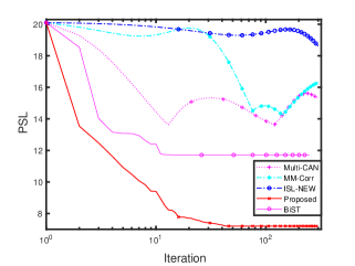
(a) Sequence set of dimension $(L,M)=(2,100)$

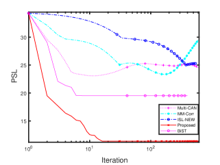
(b) Sequence set of dimension $(L,M)=(2,200)$

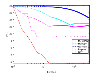
(c) Sequence set of dimension $(L,M)=(3,150)$

(d) Sequence set of dimension $(L,M)=(4,256)$

Figure 1: PSL vs Iteration

Figure. 1 show the plots of PSL value with respect to iterations for different dimensions of sequence sets $(L,M)=(2,100)$, $(L,M)=(2,200)$, $(L,M)=(3,150)$ and $(L,M)=(4,256)$. From the simulation plots, it can be seen that though all the algorithms have started at the same PSL value, they all converged to different PSL values and the proposed algorithm has reached the PSL value which is better than the state-of-the-art algorithms. For instance, from figure-1(b), one can observe that for a sequence set dimension of $(L,M)=(2,200)$, the proposed algorithm has converged to a PSL value $11$, while the state-of-the-art methods converged to $24$ (which is roughly two times more than that of the proposed method). Hence, we conclude that irrespective of sequence set dimension, our proposed algorithm exhibits better performance than the state-of-the-art algorithms in terms of PSL value.

(ii) Aperiodic correlations vs Lag

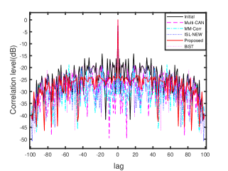
(a) $|r_{1,1}(k)|$ vs. $k$

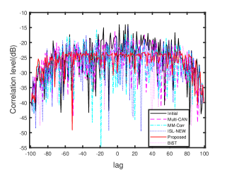
(b) $|r_{1,2}(k)|$ vs. $k$

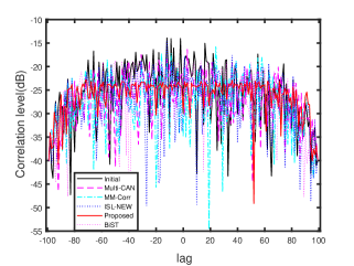
(c) $|r_{2,1}(k)|$ vs. $k$

(d) $|r_{2,2}(k)|$ vs. $k$

Figure 2: Correlations plots for sequence set design for dimensions $(L,M)=(2,100)$, please note that plots of $r_{1,2}(k)$ and $r_{2,1}(k)$ are mirror images of each other.

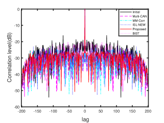
(a) $|r_{1,1}(k)|$ vs. $k$

(b) $|r_{1,2}(k)|$ vs. $k$

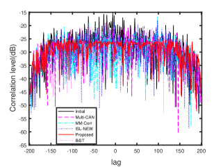
(c) $|r_{2,1}(k)|$ vs. $k$

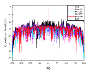
(d) $|r_{2,2}(k)|$ vs. $k$

Figure 3: Correlations plots for sequence set design for dimensions $(L,M)=(2,200)$, please note that plots of $r_{1,2}(k)$ and $r_{2,1}(k)$ are mirror images of each other.

(a) $|r_{1,1}(k)|$ vs $k$

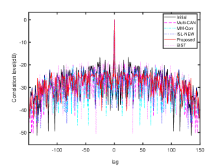
(b) $|r_{2,2}(k)|$ vs $k$

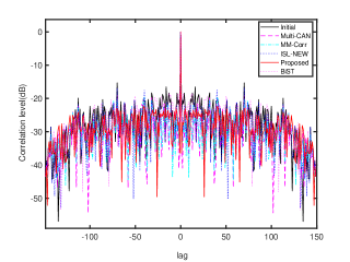
(c) $|r_{3,3}(k)|$ vs $k$

(d) $|r_{1,2}(k)|$ vs $k$

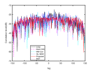
(e) $|r_{1,3}(k)|$ vs $k$

(f) $|r_{2,3}(k)|$ vs $k$

Figure 4: Correlation plots vs lag for sequence set design for dimensions $(L,M)=(3,150)$

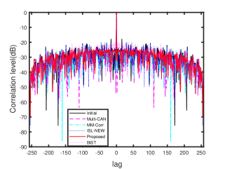
(a) $|r_{1,1}(k)|$ vs. $k$

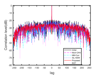
(b) $|r_{2,2}(k)|$ vs. $k$

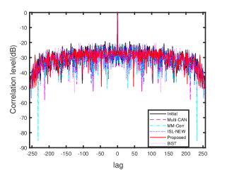
(c) $|r_{3,3}(k)|$ vs. $k$

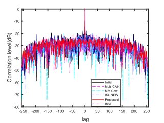
(d) $|r_{4,4}(k)|$ vs. $k$

(e) $|r_{1,2}(k)|$ vs. $k$

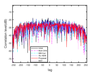
(f) $|r_{3,4}(k)|$ vs. $k$

Figure 5: Correlations plots for sequence set design for dimensions $(L,M)=(4,256)$, please note that the plots of $r_{1,3}(k)$, $r_{1,4}(k)$, $r_{2,3}(k)$, $r_{2,4}(k)$ are not included here.

Figure. 2 to Figure. 5 show the plots of correlation values (auto-correlations as well as cross-correlations) with respect to lag for different dimensions of sequence sets $(L,M)=(2,100)$, $(L,M)=(2,200)$, $(L,M)=(3,150)$ and $(L,M)=(4,256)$ respectively. From the simulation plots, we observe that, in comparison to the state-of-the-art algorithms, our proposed algorithm is performing well in terms of the PSL value and more importantly the sequences obtained via our approach have almost equi-sidelobe level (both autocorrelation and cross correlation), which is one of the main goals of our approach.

IV-B MIMO RADAR SAR IMAGING EXPERIMENT

In MIMO RADAR high-resolution imaging application [3, 32, 47], probing sequences with lower peak side-lobe level are usually preferred. So, to highlight the strength of the proposed algorithm (generated sequence set) we conduct a MIMO RADAR angle-ranging (with negligible doppler effect) experiment. Consider the colocated Uniform Linear Array (ULA) at both the transmitting and receiving ends with $4$ transmitters and $4$ receivers with inter-element spacing between the elements equal to $2\lambda$ and $\frac{\lambda}{2}$ ($\lambda$ is wavelength) respectively. If we assume that the targets are in the far-field with a simulated pattern LT occupying $Q=60$ range bins (vertical) and $P=81\,(-40^{\circ}\text{ to }40^{\circ})$ number of scanning angles (horizontal). Let $\boldsymbol{\boldsymbol{S}}$ denote the probing signal matrix, then the received data can be modeled as given as:

$$\boldsymbol{\boldsymbol{B}}^{H}=\stackrel{{\scriptstyle[}}{{r}}=0]{Q-1}{\sum}\stackrel{{\scriptstyle[}}{{p}}=1]{P}{\sum}\beta_{rp}\boldsymbol{\boldsymbol{c}}_{p}\boldsymbol{\boldsymbol{d}}_{p}^{T}\boldsymbol{\hat{\boldsymbol{S}}}^{H}\boldsymbol{\boldsymbol{J}}_{p}+\boldsymbol{\boldsymbol{N}}^{H}$$ (48)

where $\left\{\beta_{rp}\right\}_{r=0,p=1}^{Q-1,P}$ denote the radar cross sections (rcs) of the target and $\boldsymbol{\boldsymbol{d}}_{p}$, $\boldsymbol{\boldsymbol{c}}_{p}$ are the transmitting and receiving steering vectors, respectively. $\boldsymbol{\boldsymbol{J}}_{p}$ is the $p^{th}$ lag shifting matrix ( like $\boldsymbol{\boldsymbol{\boldsymbol{A}}}_{k}$ in (15)) but with dimension $\bigl{(}(M+Q-1)\times(M+Q-1)\bigr{)}$, $\boldsymbol{\boldsymbol{N}}^{H}$ is the noise matrix and $\hat{\boldsymbol{\boldsymbol{S}}}$ is the zero padded matrix which is given as $\hat{\boldsymbol{\boldsymbol{S}}}=[\boldsymbol{\boldsymbol{S}},\boldsymbol{\boldsymbol{0}}]^{T}$ ( $\boldsymbol{\boldsymbol{S}}$ is $M\times L$ dimension and $\hat{\boldsymbol{\boldsymbol{S}}}$ is $(M+Q-1)\times L$ dimension). For the experiment the target strengths $\left\{\beta_{rp}\right\}_{r=0,p=1}^{Q-1,P}$ are selected as i.i.d complex Gaussian random variables with mean $0$ and variance $1$. The steering vectors are given by:

$$\begin{array}[]{c}\boldsymbol{\boldsymbol{d}}_{p}=[1,e^{-j(4)\pi sin(\theta_{p})},e^{-j(8)\pi sin(\theta_{p})},e^{-j(12)\pi sin(\theta_{p})}]^{T}\end{array}$$ (49)

$$\begin{array}[]{c}\boldsymbol{\boldsymbol{c}}_{p}=[1,e^{-j\pi sin(\theta_{p})},e^{-j\pi 2sin(\theta_{p})},e^{-j\pi 3sin(\theta_{p})}]^{T}\end{array}$$ (50)

where $\theta_{p}$ denote the scanning angle. In the simulation, noise statistics is chosen to be i.i.d Gaussian with zero mean and variance $\sigma^{2}$. The SNR in the experiment is taken to be $30$dB ($\sigma^{2}=0.001$). To form an high resolution image, goal is to estimate $\left\{\beta_{rp}\right\}_{r=0,p=1}^{Q-1,P}$, which is done as follows. First, the matched filter $\boldsymbol{\boldsymbol{S}}_{q}^{MF}$ is applied on the received data $\boldsymbol{\boldsymbol{B}}^{H}$ to do the range compression on $q^{th}$ range bin , with the expression for filter given by:

$$\boldsymbol{\boldsymbol{S}}_{q}^{MF}=\boldsymbol{\boldsymbol{J}}_{p}^{H}\hat{\boldsymbol{\boldsymbol{S}}}(\hat{\boldsymbol{\boldsymbol{S}}}^{H}\hat{\boldsymbol{\boldsymbol{S}}})^{-1}$$ (51)

Then the filter output is given by:

$$\tilde{\boldsymbol{\boldsymbol{B}}}_{q}^{H}=\Biggl{(}\stackrel{{\scriptstyle[}}{{r}}=0]{Q-1}{\sum}\stackrel{{\scriptstyle[}}{{p}}=1]{P}{\sum}\beta_{rp}\boldsymbol{\boldsymbol{c}}_{p}\boldsymbol{\boldsymbol{d}}_{p}^{T}\boldsymbol{\hat{\boldsymbol{S}}}^{H}\boldsymbol{\boldsymbol{J}}_{p}+\boldsymbol{\boldsymbol{N}}^{H}\Biggr{)}\boldsymbol{\boldsymbol{S}}_{q}^{MF}$$ (52)

$$\begin{array}[t]{c}\tilde{\boldsymbol{\boldsymbol{B}}}_{q}^{H}=\Biggl{(}\stackrel{{\scriptstyle[}}{{p}}=1]{P}{\sum}\beta_{qp}\boldsymbol{\boldsymbol{c}}_{p}\boldsymbol{\boldsymbol{d}}_{p}^{T}+\stackrel{{\scriptstyle[}}{{r}}=0,r\neq q]{Q-1}{\sum}\stackrel{{\scriptstyle[}}{{p}}=1]{P}{\sum}\beta_{rp}\boldsymbol{\boldsymbol{c}}_{p}\boldsymbol{\boldsymbol{d}}_{p}^{T}\boldsymbol{\hat{\boldsymbol{S}}}^{H}\boldsymbol{\boldsymbol{J}}_{p}\boldsymbol{\boldsymbol{S}}_{q}^{MF}\\ +\boldsymbol{\boldsymbol{N}}^{H}\boldsymbol{\boldsymbol{S}}_{q}^{MF}\Biggr{)}\end{array}$$ (53)

The parameter of interest $\beta_{qp}$ can then be estimated in two different ways:

(a) The Least Squares Estimator:

$$\hat{\beta}_{qp}^{LS}=\frac{\boldsymbol{\boldsymbol{c}}_{p}^{H}\tilde{\boldsymbol{\boldsymbol{B}}}_{q}^{H}{\boldsymbol{\boldsymbol{d}}}_{p}}{\bigl{\|}\boldsymbol{\boldsymbol{c}}_{p}\bigr{\|}^{2}\bigl{\|}{\boldsymbol{\boldsymbol{d}}}_{p}\bigr{\|}^{2}},\,p=1,..,P,\,q=0,..,Q-1$$ (54)

(b) The CAPON Estimator:

$$\hat{\beta}_{qp}^{C}=\frac{\boldsymbol{\boldsymbol{c}}_{p}^{H}\boldsymbol{\boldsymbol{V}}_{q}^{-1}\tilde{\boldsymbol{\boldsymbol{B}}}_{q}^{H}{\boldsymbol{d}}_{p}}{\boldsymbol{\boldsymbol{c}}_{p}^{H}\boldsymbol{\boldsymbol{V}}_{q}^{-1}\boldsymbol{\boldsymbol{c}}_{p}\bigl{\|}{\boldsymbol{\boldsymbol{d}}}_{p}\bigr{\|}^{2}},\,p=1,..,P,\,q=0,..,Q-1$$ (55)

where $\boldsymbol{\boldsymbol{V}}_{q}^{-1}=\tilde{\boldsymbol{\boldsymbol{B}}}_{q}^{H}\tilde{\boldsymbol{\boldsymbol{B}}}_{q}$ is the covariance matrix of compressed received data.

The estimated $\left\{\beta_{rp}\right\}_{r=0,p=1}^{Q-1,P}$ using different probing sequences (Multi-CAN, MM-Corr, ISL-NEW, BiST ( with 8 alphabets), and the proposed algorithm) of length ($M=256$) are shown in the figures 6-7. It can be seen from the plots, for both approaches to estimate the target strengths, the sequence set generated by the proposed algorithm gives a better resolution image when compared with the images obtained by employing the sequence sets generated by other competing methods.

(a) True Target

(b) Multi-CAN sequence set

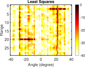
(c) MM-Corr sequence set

(d) ISL-NEW sequence set

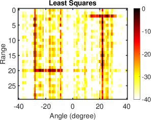
(e) BiST sequence set

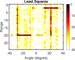
(f) Proposed sequence set

Figure 6: MIMO RADAR target image reconstruction via the Least Squares Estimation method for problem dimensions $(L,M)=(4,256)$

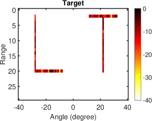
(a) True Target

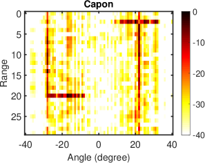
(b) Multi-CAN sequence set

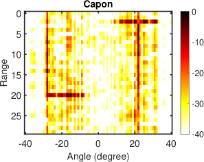
(c) MM-Corr sequence set

(d) ISL-NEW sequence set

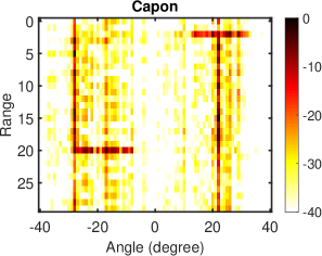
(e) BiST sequence set

(f) Proposed sequence set

Figure 7: MIMO RADAR target image reconstruction via the CAPON method for problem dimensions $(L,M)=(4,256)$

V.CONCLUSION

In this paper, we addressed the problem of designing sequence set by directly minimizing the peak side-lobe level and proposed a Majorization-Minimization technique based algorithm, which can be efficiently implemented using the FFT and IFFT operations. To evaluate the performance of the proposed algorithm, we conducted numerical simulations and compared with the state-of-the-art algorithms, and observed that the proposed algorithm is able to generate a sequence set with better PSL values. To highlight the strength of the generated sequence set, we also conduct a MIMO RADAR angle-ranging imaging experiment and showed that the sequence set designed via the proposed algorithm produces very high-resolution images when compared with the competing methods.

References

• [1] A. Hassanien and S. A. Vorobyov, “Phased-mimo radar: A tradeoff between phased-array and mimo radars,” IEEE Transactions on Signal Processing, vol. 58, no. 6, pp. 3137–3151, 2010.
• [2] R. Calderbank, S. D. Howard, and B. Moran, “Waveform diversity in radar signal processing,” IEEE Signal Process. Mag., vol. 26, no. 1, pp. 32–41, Jan 2009.
• [3] J. Li, P. Stoica, and X. Zheng, “Signal synthesis and receiver design for mimo radar imaging,” IEEE Transactions on Signal Processing, vol. 56, no. 8, pp. 3959–3968, 2008.
• [4] I. Bekkerman and J. Tabrikian, “Target detection and localization using mimo radars and sonars,” IEEE Transactions on Signal Processing, vol. 54, no. 10, pp. 3873–3883, 2006.
• [5] A. De Maio, S. De Nicola, Y. Huang, S. Zhang, and A. Farina, “Code design to optimize radar detection performance under accuracy and similarity constraints,” IEEE Transactions on Signal Processing, vol. 56, no. 11, pp. 5618–5629, 2008.
• [6] L. K. Patton, S. W. Frost, and B. D. Rigling, “Efficient design of radar waveforms for optimised detection in coloured noise,” IET Radar, Sonar Navigation, vol. 6, no. 1, pp. 21–29, 2012.
• [7] Q. He, R. S. Blum, and A. M. Haimovich, “Noncoherent mimo radar for location and velocity estimation: More antennas means better performance,” IEEE Transactions on Signal Processing, vol. 58, no. 7, pp. 3661–3680, 2010.
• [8] J. Li and P. Stoica, MIMO Radar Signal Processing.   John Wiley and Sons, 2009.
• [9] S. W. Golomb and G. Gong, Signal Design for Good Correlation: For Wireless Communication, Cryptography, and Radar.   Cambridge University Press, 2005.
• [10] H. He, J. Li, and P. Stoica, Wave form Design for Active Sensing Systems: A Computational Approach.   Cambridge University Press, 2012. [Online]. Available: https://books.google.co.in/books?id=syqYnQAACAAJ
• [11] Z. Wang, P. Babu, and D. P. Palomar, “Design of par-constrained sequences for mimo channel estimation via majorization-minimization,” IEEE Transactions on Signal Processing, vol. 64, no. 23, pp. 6132–6144, 2016.
• [12] S. Wentao, H. Jianguo, C. Xiaodong, and H. Yunshan, “Orthogonal waveforms design and performance analysis for mimo sonar,” in IEEE 10th INTERNATIONAL CONFERENCE ON SIGNAL PROCESSING PROCEEDINGS, 2010, pp. 2382–2385.
• [13] W. C. Knight, R. G. Pridham, and S. M. Kay, “Digital signal processing for sonar,” Proceedings of the IEEE, vol. 69, no. 11, pp. 1451–1506, Nov 1981.
• [14] Zhaofu Chen, J. Li, X. Tan, H. He, Bin Guo, P. Stoica, and M. Datum, “On probing waveforms and adaptive receivers for active sonar,” in OCEANS 2010 MTS/IEEE SEATTLE, Sep. 2010, pp. 1–10.
• [15] J. Liang, L. Xu, J. Li, and P. Stoica, “On designing the transmission and reception of multistatic continuous active sonar systems,” IEEE Transactions on Aerospace and Electronic Systems, vol. 50, no. 1, pp. 285–299, 2014.
• [16] J. Ling, T. Yardibi, X. Su, H. He, and J. Li, “Enhanced channel estimation and symbol detection for high speed mimo underwater acoustic communications,” in 2009 IEEE 13th Digital Signal Processing Workshop and 5th IEEE Signal Processing Education Workshop, 2009, pp. 126–131.
• [17] N. Suehiro, “A signal design without co-channel interference for approximately synchronized cdma systems,” IEEE Journal on Selected Areas in Communications, vol. 12, no. 5, pp. 837–841, 1994.
• [18] J. Oppermann and B. S. Vucetic, “Complex spreading sequences with a wide range of correlation properties,” IEEE Transactions on Communications, vol. 45, no. 3, pp. 365–375, 1997.
• [19] S. E. Kocabas and A. Atalar, “Binary sequences with low aperiodic autocorrelation for synchronization purposes,” IEEE Communications Letters, vol. 7, no. 1, pp. 36–38, Jan 2003.
• [20] J. Khalife, K. Shamaei, and Z. M. Kassas, “Navigation with cellular cdma signals part i: Signal modeling and software-defined receiver design,” IEEE Transactions on Signal Processing, vol. 66, no. 8, pp. 2191–2203, 2018.
• [21] R. Barker, “Group synchronizing of binary digital systems,” Academic Press, New York, 1953.
• [22] N. Zhang and S. W. Golomb, “Polyphase sequence with low autocorrelations,” IEEE Transactions on Information Theory, vol. 39, no. 3, pp. 1085–1089, May 1993.
• [23] R. Frank, “Polyphase codes with good nonperiodic correlation properties,” IEEE Transactions on Information Theory, vol. 9, no. 1, pp. 43–45, January 1963.
• [24] P. Borwein and R. Ferguson, “Polyphase sequences with low autocorrelation,” IEEE Transactions on Information Theory, vol. 51, no. 4, pp. 1564–1567, April 2005.
• [25] J. Song, P. Babu, and D. P. Palomar, “Optimization methods for designing sequences with low autocorrelation sidelobes,” IEEE Transactions on Signal Processing, vol. 63, no. 15, pp. 3998–4009, Aug 2015.
• [26] J. Song, P. Babu, and D. P. Palomar, “Sequence design to minimize the weighted integrated and peak sidelobe levels,” IEEE Transactions on Signal Processing, vol. 64, no. 8, pp. 2051–2064, April 2016.
• [27] M. A. Kerahroodi, A. Aubry, A. De Maio, M. M. Naghsh, and M. Modarres-Hashemi, “A coordinate-descent framework to design low psl/isl sequences,” IEEE Transactions on Signal Processing, vol. 65, no. 22, pp. 5942–5956, 2017.
• [28] W. Fan, J. Liang, H. C. So, and G. Lu, “Min-max metric for spectrally compatible waveform design via log-exponential smoothing,” IEEE Transactions on Signal Processing, vol. 68, pp. 1075–1090, 2020.
• [29] W. Fan, J. Liang, G. Yu, H. C. So, and G. Lu, “Minimum local peak sidelobe level waveform design with correlation and/or spectral constraints,” Signal Process., vol. 171, p. 107450, 2020.
• [30] L. Wu and D. P. Palomar, “Sequence design for spectral shaping via minimization of regularized spectral level ratio,” IEEE Transactions on Signal Processing, vol. 67, no. 18, pp. 4683–4695, 2019.
• [31] A. Aubry, A. De Maio, B. Jiang, and S. Zhang, “Ambiguity function shaping for cognitive radar via complex quartic optimization,” IEEE Transactions on Signal Processing, vol. 61, no. 22, pp. 5603–5619, 2013.
• [32] H. He, P. Stoica, and J. Li, “Designing unimodular sequence sets with good correlations-including an application to mimo radar,” IEEE Transactions on Signal Processing, vol. 57, no. 11, pp. 4391–4405, 2009.
• [33] J. Song, P. Babu, and D. P. Palomar, “Sequence set design with good correlation properties via majorization-minimization,” IEEE Transactions on Signal Processing, vol. 64, no. 11, pp. 2866–2879, 2016.
• [34] Y. Li and S. A. Vorobyov, “Fast algorithms for designing unimodular waveform(s) with good correlation properties,” IEEE Transactions on Signal Processing, vol. 66, no. 5, pp. 1197–1212, March 2018.
• [35] H. Esmaeili-Najafabadi, M. Ataei, and M. F. Sabahi, “Designing sequence with minimum psl using chebyshev distance and its application for chaotic mimo radar waveform design,” IEEE Transactions on Signal Processing, vol. 65, no. 3, pp. 690–704, 2017.
• [36] G. Cui, X. Yu, M. Piezzo, and L. Kong, “Constant modulus sequence set design with good correlation properties,” Signal Processing, vol. 139, pp. 75 – 85, 2017. [Online]. Available: http://www.sciencedirect.com/science/article/pii/S0165168417301378
• [37] M. Alaee-Kerahroodi, M. Modarres-Hashemi, and M. M. Naghsh, “Designing sets of binary sequences for mimo radar systems,” IEEE Transactions on Signal Processing, vol. 67, no. 13, pp. 3347–3360, 2019.
• [38] M. Alaee-Kerahroodi, M. R. Bhavani Shankar, K. V. Mishra, and B. Ottersten, “Meeting the lower bound on designing set of unimodular sequences with small aperiodic/periodic isl,” in 2019 20th International Radar Symposium (IRS), 2019, pp. 1–13.
• [39] J. Leeuw and W. Heiser, “Convergence of correction matrix algorithms for multidimensional scaling,” 1977.
• [40] D. R. Hunter and K. Lange, “A tutorial on mm algorithms,” The American Statistician, vol. 58, no. 1, pp. 30–37, 2004. [Online]. Available: https://doi.org/10.1198/0003130042836
• [41] Y. Sun, P. Babu, and D. P. Palomar, “Majorization-minimization algorithms in signal processing, communications, and machine learning,” IEEE Transactions on Signal Processing, vol. 65, no. 3, pp. 794–816, Feb 2017.
• [42] S. Boyd, S. P. Boyd, and L. Vandenberghe, Convex optimization.   Cambridge university press, 2004.
• [43] M. Grant and S. Boyd, “CVX: Matlab software for disciplined convex programming, version 2.1,” http://cvxr.com/cvx, Mar. 2014.
• [44] J. Von Neumann and O. Morgenstern, Theory of Games and Economic Behavior, ser. Science Editions.   Princeton University Press, 1944. [Online]. Available: https://books.google.co.in/books?id=AUDPAAAAMAAJ
• [45] A. Beck and M. Teboulle, “Mirror descent and nonlinear projected subgradient methods for convex optimization,” Oper. Res. Lett., vol. 31, no. 3, pp. 167–175, May 2003.
• [46] D. Bertsekas, A. Nedić, and A. Ozdaglar, Convex Analysis and Optimization, ser. Athena Scientific optimization and computation series.   Athena Scientific, 2003. [Online]. Available: https://books.google.co.in/books?id=DaOFQgAACAAJ
• [47] W. Roberts, P. Stoica, J. Li, T. Yardibi, and F. A. Sadjadi, “Iterative adaptive approaches to mimo radar imaging,” IEEE Journal of Selected Topics in Signal Processing, vol. 4, no. 1, pp. 5–20, 2010.