Estimation of Structural Causal Model
via Sparsely Mixing Independent Component Analysis

Abstract

We consider the problem of inferring the causal structure from observational data, especially when the structure is sparse. This type of problem is usually formulated as an inference of a directed acyclic graph (DAG) model. The linear non-Gaussian acyclic model (LiNGAM) is one of the most successful DAG models, and various estimation methods have been developed. However, existing methods are not efficient for some reasons: (i) the sparse structure is not always incorporated in causal order estimation, and (ii) the whole information of the data is not used in parameter estimation. To address these issues, we propose a new estimation method for a linear DAG model with non-Gaussian noises. The proposed method is based on the log-likelihood of independent component analysis (ICA) with two penalty terms related to the sparsity and the consistency condition. The proposed method enables us to estimate the causal order and the parameters simultaneously. For stable and efficient optimization, we propose some devices, such as a modified natural gradient. Numerical experiments show that the proposed method outperforms existing methods, including LiNGAM and NOTEARS.

It has been a significant topic to search for causal relationships from observational data in various scientific fields, such as biology (Sachs et al. 2005), economy (Hoover 2008), and psychology (Glymour 1998). To detect causal relationships, graphical models have been used, in which directed edges represent causal relationships. In particular, a Directed Acyclic Graph (DAG) has been intensively studied for years. There are some traditional approaches for learning a DAG, like PC algorithm (Spirtes et al. 2000) and GES algorithm (Chickering 2002). These can produce a Markov equivalence class, which contains all DAGs consistent with the conditional independence of the data, but cannot always identify a complete causal structure (Spirtes et al. 2000; Judea 2000) .

This problem has been overcome by Shimizu et al. (2006), Zhang and Hyvärinen (2009), Peters and Bühlmann (2014), and Peters et al. (2014). They constructed fully-identifiable DAG models by some additional assumptions. In particular, the Linear Non-Gaussian Acyclic Model (LiNGAM) proposed by Shimizu et al. (2006) has many applications in various fields (e.g. Liu et al. 2015; von Eye and DeShon 2012; Xu 2017), by virtue of good interpretability and relatively mild assumptions, compared to the other identifiable linear DAG models.

Shimizu et al. (2006) also proposed an estimation method based on Independent Component Analysis (ICA). Recently, some other estimation methods for LiNGAM were proposed: DirectLiNGAM (Shimizu et al. 2011), Pairwise LiNGAM (Hyvärinen and Smith 2013), and High-dimensional LiNGAM (Wang and Drton 2020). These methods, including the original LiNGAM, consist of two stages, causal order estimation and parameter estimation.

Here, we focus on a sparse structure of causal relationships in high-dimensional data. The two-stage methods are not efficient in this case for two reasons: (i) the sparse structure is not always incorporated in causal order estimation, and (ii) the whole information of the data is not used in parameter estimation. To address these issues, we propose a new one-stage method based on LiNGAM with sparsity. Based on the whole information of the data, the method estimates the causal order and the parameters simultaneously. A sparse estimation method based on LiNGAM was already discussed by Zhang and Chan (2006) and Zhang et al. (2009). However, their methods do not satisfy the consistency conditions of the optimal solution. This paper addresses this issue by a devised penalty related to the consistency condition. These issues motivate us to develop a one-stage algorithm incorporating the sparse structure.

In this paper, we formulate a one-stage estimation method for LiNGAM with a sparse penalty and a devised penalty related to the consistency condition of the optimal solution. Then, we make an efficient optimization algorithm that modifies a widely-used ADMM algorithm with a devised expression and a modified natural gradient descent. We also propose an objective procedure for selecting a tuning parameter via the likelihood cross validation (CV). In addition, we demonstrate the effectiveness and scalability of the proposed method through numerical experiments. The proposed method is compared with some estimation methods of LiNGAM and another approach NOTEARS (Zheng et al. 2018). The proposed method outperforms others in almost all cases and shows stable performance even in high dimensional cases. The scalability of the proposed method is examined. The proposed method is also applied to real data.

Problem and Related Works

Linear DAG Model

Suppose that $X=(X_{1},\ldots,X_{d})^{T}$ is a $d$-dimensional random vector drawn from the joint distribution $P(X)$. We assume ${\rm E}[X]=0$ without loss of generality. A Directed Acyclic Graph (DAG) model on $X$ can be defined by $P(X)$ and a DAG $G=(V_{G},E_{G})$, where $V_{G}$ and $E_{G}$ are the sets of vertices and directed edges, respectively. The vertices in $V_{G}$ correspond to the indices of $X$. The element $(j,k)\in E_{G}$ shows a directed edge from $j$ to $k$, which represents the direct causal relationship from $X_{j}$ to $X_{k}$. The acyclicity implies no directed cycles in $G$.

This paper focuses on a linear DAG model. A linear DAG model is equivalent to a linear structural equation given by

$$X_{j} =\mathbf{b}_{j}^{T}X+S_{j},\qquad j=1,\ldots,d,$$ (1)

where $\mathbf{b}_{j}=(b_{j1},\ldots,b_{jd})^{T}$ is a coefficient parameter vector and $S=(S_{1},\ldots,S_{d})^{T}$ is an independent noise vector. Suppose that $(j,k)\not\in E_{G}$ if $b_{kj}=0$ and $(j,k)\in E_{G}$ if $b_{kj}\neq 0$, which defines the structure of $G$. The above equation can also be expressed in matrix form:

$$X=\mathbf{B}X+S,$$ (2)

where $\mathbf{B}=(\mathbf{b}_{1},\ldots,\mathbf{b}_{d})^{T}$ is called the weighted adjacency matrix in graph theory. From the acyclicity, all the diagonal entries of $\mathbf{B}$ are zero and $X_{1},\ldots,X_{d}$ can be rearranged in a causal order. Let $\pi(j)$ be the index of $X_{j}$ permuted in a causal order, and then we have $\pi(j)<\pi(k)$ for any edges $(\pi(j),\pi(k))\in E_{G}$. The corresponding permutation matrix $\mathbf{P}$ can transform $\mathbf{B}$ by $\mathbf{PBP}^{T}$ to a strictly lower triangular matrix (Shimizu et al. 2006; Bollen 1989).

Suppose that we have the data $\mathbf{X}\in\mathbb{R}^{N\times d}$ with $N$ random samples drawn from $P(X)$. The problem is to estimate the parameter matrix $\mathbf{B}$ from the data $\mathbf{X}$. The difficulty in the problem is that $\mathbf{B}$ must be transformed by a permutation to a lower triangular matrix due to the acyclicity.

LiNGAM and Its Estimation

LiNGAM (Shimizu et al. 2006) is a linear DAG model with non-Gaussian noises, which is proved to be fully identifiable via Independent Component Analysis (ICA). The linear DAG model can be expressed by

$$X=\mathbf{M}^{-1}S,\qquad\mathbf{M}=\mathbf{I}-\mathbf{B},$$ (3)

which can be seen as an ICA model with the mixture matrix $\mathbf{M}^{-1}$. In the ICA model, the matrix $\mathbf{M}$ is identifiable up to the scaling and the permutation of its rows. This indeterminacy is not a problem in ICA, but a crucial problem in causal discovery. This problem can be solved using the acyclicity of $G$, as described in Shimizu et al. (2006).

Shimizu et al. (2006) also constructed the parameter estimation algorithm, ICA-LiNGAM. This algorithm is summarized as follows. First, the parameter estimate $\hat{\mathbf{M}}_{ICA}$ is obtained by a standard ICA algorithm like FastICA (Hyvärinen 1999). Second, the rows of $\hat{\mathbf{M}}_{ICA}$ are permuted so that its diagonal entries are far from zero as possible, and then each row is rescaled by its corresponding diagonal entry. Let $\hat{\mathbf{M}}$ be the permuted and rescaled matrix. Third, the causal order is explored by minimizing the squared sum of upper-triangular entries of $\hat{\mathbf{B}}~{}(=\mathbf{I}-\hat{\mathbf{M}})$. Here, there is a big problem that the third step is computationally infeasible even when $d$ is not large. In order to avoid this problem, non-zero entries with small absolute values in $\hat{\mathbf{B}}$ are sequentially truncated to zero until $\hat{\mathbf{B}}$ can be transformed into a lower triangular matrix. After the transformation, $X$ is rearranged in a causal order. Finally the parameter is estimated again by sparse linear regression along with the determined ordering (Wiedermann and Von Eye 2016; Zou 2006).

Zhang and Chan (2006) and Zhang et al. (2009) proposed another approach based on the log-likelihood of ICA with a sparse penalty. However, it does not satisfy the consistency conditions of independent components, as discussed later, so that the parameter estimation is considered to be unstable. In addition, the subgradient of the sparse penalty is approximated by a continuous function, and thereby the estimate is not always shrunk to zero. This paper adopts this line, but develops the penalty term to meet the consistency assumptions and essentially improves the parameter estimation algorithm to make it stable and obtain exact sparsity.

A different approach from ICA-based methods was employed in DirectLiNGAM (Shimizu et al. 2011), Pairwise LiNGAM (Hyvärinen and Smith 2013), and High-dimensional LiNGAM (Wang and Drton 2020). These methods evaluate the causal order of variable pairs and then integrate them to obtain a global causal order. Next, they estimate the parameter in the same manner as that of ICA-LiNGAM. These approaches are preferable because the solution can be obtained in finite steps in contrast to the iterative algorithms. However, there are two difficulties in this line. The first one is that the causal order estimation is not efficient because the sparse structure of $\mathbf{B}$ is not incorporated, except for Wang and Drton (2020). The second one is that the parameter estimation of this approach is based on the least squares. This means the assumptions of non-Gaussianity is not used in parameter estimation, so that the efficiency may be reduced due to the information loss.

NOTEARS

Zheng et al. (2018) introduced a new characterization of ”DAGness” using a continuous function $h:\mathbb{R}^{d\times d}\rightarrow\mathbb{R}$ such that $h(\mathbf{B})=0$ if and only if the graph is acyclic. The function $h$ enables us to obtain DAG via totally continuous optimization, although the structure of DAG was explored via combinatorial optimization in the past. Using the function $h$, they proposed a novel structure learning method by the following continuous optimization problem:

$$\begin{array}[]{c}\displaystyle\min_{\mathbf{B}\in\mathbb{R}^{d\times d}}\quad{\frac{1}{2N}}\|\mathbf{X}-\mathbf{XB}^{T}\|_{F}^{2}+\lambda\|\mathbf{B}\|_{1}\\ \text{subject to}\quad h(\mathbf{B})=0.\end{array}$$ (6)

This was called Non-combinatorial Optimization via Trace Exponential and Augmented lagRangian for Structure learning (NOTEARS).

NOTEARS does not assume any conditions on noises except for independence. However, we suspect this assumption because the linear DAG model is not identifiable without some additional conditions (Spirtes et al. 2000); e.g., if the noises are assumed to be Gaussian with equal variances and the squared error in (6) is replaced by the negative log-likelihood of Gaussian noises, the linear DAG model is identifiable (Peters and Bühlmann 2014). This assumption, in particular, the assumption of equal variances, will be much stronger in real-world data than the non-Gaussian assumption in LiNGAM.

Parameter Estimation

In this section, we propose a new method, which we call sparsely mixing ICA-LiNGAM (sICA-LiNGAM), for estimating the linear DAG model with non-Gaussian noises. The parameter is estimated using the log-likelihood of ICA with two penalties. Although a usual ICA method needs the orthogonality of the parameter matrix, it will not work well with a sparse penalty, as described later. To address this issue, we introduced a devised penalty.

ICA and Consistent Estimation

Here we briefly review the ICA and its consistent estimation. Let $S=(S_{1},\ldots,S_{d})^{T}$ be the vector of independent components (ICs) with zero means. Suppose that we observe $X={\mathbf{A}}S$. The purpose of ICA is to recover the ICs $S$ by ${\mathbf{M}}X$, where $\mathbf{M}$ is the parameter matrix.

Let $p_{j}$ be the probability density function of $S_{j}$ and let $\mathbf{M}=(\boldsymbol{m}_{1},\ldots,\boldsymbol{m}_{d})^{T}$ and $\mathbf{X}=(\boldsymbol{x}_{1},\ldots,\boldsymbol{x}_{N})^{T}$. The maximum likelihood estimator (MLE) $\hat{\mathbf{M}}$ is given by

$$\hat{\mathbf{M}}= \arg\max_{\mathbf{M}}\ell(\mathbf{M};\mathbf{X}),$$ (7)

$$\ell(\mathbf{M};\mathbf{X})= \frac{1}{N}\sum_{i=1}^{N}\sum_{j=1}^{d}\log p_{j}(\boldsymbol{m}_{j}^{T}\boldsymbol{x}_{i})+\log|\det\mathbf{M}|.$$ (8)

In ICA, we assume that $p_{j}$s are unknown, so that it seems impossible to estimate $\mathbf{M}$ consistently. However, even when $p_{j}$s are unknown, the following theorem tells that MLE has consistency except for the indeterminacy of the scale and the order of the estimated ICs if we use appropriate probability density functions $\tilde{p}_{j}$s instead of $p_{j}$s.

Theorem 1 (Hyvärinen, Karhunen, and Oja (2001))

Let $Y_{j}=\boldsymbol{m}_{j}^{T}X$ be the estimated ICs. Suppose that $Y_{j}$s are uncorrelated with unit variance. The MLE $\hat{\mathbf{M}}$ has consistency except for the indeterminacy of the scale and the order of ICs, if

$$\mathbb{E}[S_{j}(\tilde{g}_{j}(S_{j}))-\tilde{g}_{j}^{\prime}(S_{j})]>0\quad\text{for }j=1,\ldots,d,$$ (9)

where

$$\tilde{g}_{j}(S_{j})=\frac{\partial}{\partial S_{j}}\log\tilde{p}_{j}(S_{j}).$$ (10)

Pre-whitening is often employed in ICA algorithms to convert the assumptions on $Y_{j}$s in Theorem 1 into a convenient parameter constraint. Consider the spectral decomposition of $(1/N)\mathbf{X}^{T}\mathbf{X}=\mathbf{VD}^{2}\mathbf{V}^{T}$, where $\mathbf{V}$ is the orthogonal matrix and $\mathbf{D}^{2}$ is the diagonal matrix whose diagonal entries are the eigenvalues of $(1/N)\mathbf{X}^{T}\mathbf{X}$. Let

$$\mathbf{Z}=(\mathbf{z}_{1},\ldots,\mathbf{z}_{N})^{T}=\mathbf{X}\mathbf{V}\mathbf{D}^{-1},$$ (11)

where the diagonal elements of $\mathbf{D}$ are non-negative. Then we have $(1/N)\mathbf{Z}^{T}\mathbf{Z}=I_{d}$, so that the transformed variable $\mathbf{Z}$ is uncorrelated with unit variance before estimation. Let $\mathbf{W}=\mathbf{MVD}$. Therefore, the MLE of $\mathbf{W}$ is given by

$$\hat{\mathbf{W}}= \arg\max_{\mathbf{W}}\tilde{\ell}(\mathbf{W};\mathbf{Z}),$$ (12)

$$\tilde{\ell}(\mathbf{W};\mathbf{Z})= \frac{1}{N}\sum_{i=1}^{N}\sum_{j=1}^{d}\log p_{j}(\boldsymbol{w}_{j}^{T}\boldsymbol{z}_{i})+\log|\det\mathbf{W}|,$$ (13)

where $\boldsymbol{w}_{j}$ is the $j$th row of $\mathbf{W}$. We also have $\hat{\mathbf{M}}=\hat{\mathbf{W}}\mathbf{D}^{-1}\mathbf{V}^{T}$.

Let $Y_{ij}=\boldsymbol{m}^{T}_{j}\boldsymbol{x}_{i}$ and $\mathbf{Y}=(Y_{ij})\in\mathbb{R}^{N\times d}$. We have $\mathbf{Y}=\mathbf{XM}^{T}=\mathbf{ZW}^{T}$. Here, we suppose $\mathbf{W}$ is an orthogonal matrix. Considering the pre-whitening, the orthogonality of $\mathbf{W}$ keeps $\mathbf{Y}$ whitened:

$$\frac{1}{N}\mathbf{Y}^{T}\mathbf{Y}=\mathbf{W}\left(\frac{1}{N}\mathbf{Z}^{T}\mathbf{Z}\right)\mathbf{W}^{T}=\mathbf{W}\mathbf{W}^{T}=\mathbf{I}.$$ (14)

This implies that if we assume $\mathbf{W}$ is an orthogonal matrix, the estimated ICs are whitened even in a finite sample. Many ICA algorithms efficiently obtain $\hat{\mathbf{W}}$ by utilizing this orthogonality (Hyvärinen, Karhunen, and Oja 2001). However, (14) should hold at the population level, as seen in Theorem 1, and hence the orthogonality constraint is not necessary to be satisfied strictly in a finite sample. In addition, a strict orthogonality constraint will be difficult to meet a sparse estimation, as mentioned later, and therefore we relax this constraint as a penalty term, as described later.

ICA with Sparse Penalty for Causal Discovery

Returning to the linear DAG estimation, we consider the sparse structure of $\mathbf{M}$, because the half of the entries of $\mathbf{M}~{}(=\mathbf{I}-\mathbf{B})$ should be zero due to the acyclicity. In addition, the causal structure may be simple, which also implies $\mathbf{M}$ has a sparse structure. We add to the log-likelihood (13) a sparse penalty of the adaptive lasso (Zou 2006):

$$\mathcal{P}_{\gamma}(\mathbf{M})=\sum_{j,k=1}^{d}c_{jk}^{\gamma}|m_{jk}|,\quad c_{jk}>0.$$ (15)

A typical example of the weight is $c_{jk}=1/|m_{jk}^{0}|$, where $m_{jk}^{0}$ is an initial estimator for $m_{jk}$. A candidate for $m_{jk}^{0}$ is the MLE or the estimate at a small penalty with $c_{jk}^{\gamma}=1$. The tuning parameter $\gamma$ can be selected by cross-validation. However, we employ $\gamma=1$ for simplicity, which was used in some relevant papers (Zhang et al. 2009; Hyvärinen et al. 2010). Unfortunately, we cannot impose sparsity on $\mathbf{B}$ directly because the MLE cannot identify the order of ICs, and $\mathbf{B}$ cannot be derived correctly. In this paper, the order of the ICs is decided in a similar way to ICA-LiNGAM.

Here we review the principal component analysis (PCA) with sparsity. The PCs are obtained under orthogonality constraint. This situation is similar to that discussed above. Jolliffe, Trendafilov, and Uddin (2003) proposed a method for obtaining sparse PCs by the maximizing the explained variances with an $L_{1}$ penalty under orthogonality constraint. Zou, Hastie, and Tibshirani (2006) reported that it was difficult to obtain sufficiently sparse PCs by the method of Jolliffe, Trendafilov, and Uddin (2003), and then they proposed a smart idea to obtain sparse PCs. Unfortunately, such an idea cannot be applied to our situation. The most important message is that the sparse penalty may not work well under the orthogonality constraint. To address this issue, a novel method is proposed in this paper, which contains an additional penalty related to the orthogonality constraint.

In order to obtain a sparse structure on $\mathbf{M}$, we relax the orthogonality constraint on $\mathbf{W}$. More precisely, we impose a unit-norm constraint on each row of $\mathbf{W}$ and relax the off-diagonal orthogonality constraint by adding a new penalty term $\|\mathbf{P}^{T}\mathbf{W}-\mathbf{I}\|_{F}^{2}$ with $\mathbf{P}^{T}\mathbf{P}=\mathbf{I}$ to the objective function. Note that the additional penalty term implies the orthogonality constraint because the minimizer of $\|\mathbf{P}^{T}\mathbf{W}-\mathbf{I}\|_{F}^{2}$ under $\mathbf{P}^{T}\mathbf{P}=\mathbf{I}$ satisfies $\mathbf{W}^{T}\mathbf{W}=\mathbf{I}$.

Finally, we summarize the proposed method. The objective function consists of the log-likelihood (13), the adaptive lasso penalty (15), and the orthogonality penalty $\|\mathbf{P}^{T}\mathbf{W}-I\|_{F}^{2}$ with $\mathbf{P}^{T}\mathbf{P}=I$. Denote the objective function by

$$\begin{array}[]{l}F(\mathbf{W})=-\tilde{\ell}(\mathbf{W};\mathbf{X})\\ \qquad+\lambda\left\{\alpha\mathcal{P}_{\gamma}(\mathbf{WD}^{-1}\mathbf{V}^{T})+\frac{(1-\alpha)}{2}\|\mathbf{P}^{T}\mathbf{W}-\mathbf{I}\|_{F}^{2}\right\}.\end{array}$$ (18)

Let $\mathcal{N}\subset\mathbb{R}^{d\times d}$ be the set of non-singular matrices whose row vectors are normalized. The parameter estimation is defined by

$$\begin{array}[]{cc}\displaystyle\hat{\mathbf{W}}=\min_{\mathbf{W}\in\mathcal{N}}F(\mathbf{W})\qquad\text{subject to}\quad\mathbf{P}^{T}\mathbf{P}=\mathbf{I}.\end{array}$$ (20)

The probability density functions $\tilde{p}_{j}$s are adaptively selected between two candidates, as seen in Hyvärinen, Karhunen, and Oja (2001). After estimating $\mathbf{M}$ by $\hat{\mathbf{M}}=\hat{\mathbf{W}}\mathbf{D}^{-1}\mathbf{V}^{T}$, we recover the causal order of the variables. The estimation algorithms for the parameters and the causal order are described in the next section.

Note that each column of $\mathbf{X}$ is centered and normalized before obtaining $\mathbf{V}$ and $\mathbf{D}$, as adopted for a usual lasso. The tuning parameter $\lambda$ controls the total extent of the penalty, and $\alpha$ balances the sparsity and the orthogonality.

Algorithm

In this section, we show the whole algorithm of the proposed method. First, we show how to obtain the minimizer $\hat{\mathbf{W}}$ with given tuning parameters $\lambda$ and $\alpha$. Next, we illustrate how to select the tuning parameters. Finally, we explain how to estimate the causal order of variables.

How to Obtain Parameter Estimates

We derive an optimization algorithm based on the Alternating Direction Method of Multipliers (ADMM; Boyd, Parikh, and Chu 2011). ADMM is applied to the optimization of the objective function $f_{1}(x)+f_{2}(z)$ under a linear constraint on $(x,z)$. In particular, ADMM is a strong tool when one of two functions is simple, and then ADMM is widely used to solve a sparse estimation problem.

First, the optimization problem (20) is equivalently transformed to the ADMM form:

$$\begin{array}[]{cc}\displaystyle\min_{\mathbf{W}\in\mathcal{N},\mathbf{M,P}\in\mathbb{R}^{d\times d}}F_{1}(\mathbf{W},\mathbf{P})+F_{2}(\mathbf{M})\\ \text{subject to}\quad\mathbf{WD}^{-1}\mathbf{V}^{T}=\mathbf{M},~{}\mathbf{P}^{T}\mathbf{P}=\mathbf{I},\end{array}$$ (23)

where

$$F_{1}(\mathbf{W},\mathbf{P}) =-\tilde{\ell}(\mathbf{W};\mathbf{X})+\lambda\frac{(1-\alpha)}{2}\|\mathbf{P}^{T}\mathbf{W}-\mathbf{I}\|_{F}^{2},$$

$$F_{2}(\mathbf{M}) =\lambda\alpha\mathcal{P}_{\gamma}(\mathbf{M}).$$

Then, we update $(\mathbf{W},\mathbf{M})$ and $\mathbf{P}$ alternately. For given $\mathbf{W}$ (and $\mathbf{M}$), the updated matrix of $\mathbf{P}$ is obtained by minimizing $\|\mathbf{P}^{T}\mathbf{W}-\mathbf{I}\|_{F}^{2}$ under $\mathbf{P}^{T}\mathbf{P}=\mathbf{I}$. Let the singular value decomposition of $\mathbf{W}$ be denoted by $\mathbf{U}_{W}\mathbf{D}_{W}\mathbf{V}_{W}^{T}$. We see that the updated matrix of $\mathbf{P}$ is given by $\mathbf{P}=\mathbf{U}_{W}\mathbf{V}_{W}^{T}$. (Mardia, Kent, and Bibby 1979). For given $\mathbf{P}$, the augmented Lagrangian is given by

$$\mathcal{L}_{\rho}(\mathbf{W},\mathbf{M},\mathbf{U})=F_{1}(\mathbf{W},\mathbf{P})+F_{2}(\mathbf{M})$$ (24)

$$\ \ +\mathrm{tr}\left[\mathbf{U}^{T}(\mathbf{WD}^{-1}\mathbf{V}^{T}-\mathbf{M})\right]+\frac{\rho}{2}\|\mathbf{WD}^{-1}\mathbf{V}^{T}-\mathbf{M}\|_{F}^{2},$$

where $\mathbf{U}\in\mathbb{R}^{d\times d}$ is a Lagrange multiplier matrix and $\rho$ is a tuning parameter. From the optimality condition of ADMM, the updates of $\mathbf{W},\mathbf{M},\text{and}~{}\mathbf{U}$ are given by

$$\left\{\begin{array}[]{l}\displaystyle\mathbf{W}_{t+1}=\mathrm{arg}\min_{\mathbf{W}\in\mathcal{N}}\mathcal{L}_{\rho}(\mathbf{W},\mathbf{M}_{t},\mathbf{U}_{t})\\ \displaystyle\mathbf{M}_{t+1}=\mathrm{arg}\min_{\mathbf{M}\in\mathbb{R}^{d\times d}}\mathcal{L}_{\rho}(\mathbf{W}_{t+1},\mathbf{M},\mathbf{U}_{t})\\ \displaystyle\mathbf{U}_{t+1}=\mathbf{U}_{t}+\rho(\mathbf{W}_{t+1}\mathbf{D}^{-1}\mathbf{V}^{T}-\mathbf{M}_{t+1})\end{array}\right.,$$ (28)

In the following, the first and second updates are discussed in detail.

Algorithm 1 Gradient Descent for $\mathbf{W}$

1:Input:
$\mathbf{W}_{t}$, $\mathcal{L}_{\rho}(\mathbf{W},\mathbf{M}_{t},\mathbf{U}_{t})$, $u_{\mathrm{max}}$, and learning rate $\eta>0$

2:Output: $\mathbf{W}_{t+1}$

3:Calculate the natural gradient $\Delta\tilde{\mathbf{W}}$ and its modification $\Delta{\mathbf{W}}$.

4:for $u=1$ to $u_{\mathrm{max}}$ do

5:     $\mathbf{W}_{t}^{(u+1)}\leftarrow\mathbf{W}_{t}^{(u)}-\eta\Delta\mathbf{W}$

6:     break if the convergence criteria for $\mathbf{W}$ is satisfied. end for

7:Update $\mathbf{W}$ as $\mathbf{W}_{t+1}\leftarrow\mathbf{W}_{t}^{(u_{\mathrm{max}})}$

8:$\boldsymbol{w}_{j,t+1}\leftarrow\boldsymbol{w}_{j,t+1}/\|\boldsymbol{w}_{j,t+1}\|$ for all $j$

The first update in (28) is based on the gradient descent in Algorithm 1. The key is the gradient $\Delta\mathbf{W}$. We use the natural gradient (Amari 1998), given by

$$\Delta\tilde{\mathbf{W}} =\frac{\partial\mathcal{L}_{\rho}(\mathbf{W},\mathbf{M}_{t},\mathbf{U}_{t})}{\partial\mathbf{W}}\mathbf{W}^{T}\mathbf{W}$$

$$=-\left(\frac{1}{N}\sum_{i=1}^{N}\sum_{j=1}^{d}\tilde{g}(\boldsymbol{w}_{j}^{T}\boldsymbol{z}_{i})\boldsymbol{w}_{j}^{T}\boldsymbol{z}_{i}+\mathbf{I}\right)\mathbf{W}$$

$$\quad+\lambda\frac{(1-\alpha)}{2}(\mathbf{W}-\mathbf{P})\mathbf{W}^{T}\mathbf{W}$$ (29)

$$\quad+\left\{\mathbf{U}_{t}+\rho(\mathbf{W}\mathbf{D}^{-1}\mathbf{V}^{T}-\mathbf{M}_{t})\right\}\mathbf{VD}^{-1}\mathbf{W}^{T}\mathbf{W}.$$

The problem is that the updated matrix using the natural gradient is usually not in $\mathcal{N}$, so that we must make a gradient such that the updated matrix is in $\mathcal{N}$. Consider a small change $\mathbf{W}+\varepsilon\Delta\mathbf{W}~{}(\varepsilon>0)$. When it is in $\mathcal{N}$, the diagonal entries of $(\mathbf{W}+\varepsilon\Delta\mathbf{W})(\mathbf{W}+\varepsilon\Delta\mathbf{W})^{T}$ must be one. Here we ignore a very small term related to $\varepsilon^{2}$, which yields $\mathrm{diag}(\mathbf{W}\Delta\mathbf{W}^{T})=\mathbf{0}$. Let $\Delta\mathbf{W}=(\delta\boldsymbol{w}_{1},\ldots,\delta\boldsymbol{w}_{d})^{T}$ with

$$\delta\boldsymbol{w}_{j} =\delta\tilde{\boldsymbol{w}}_{j}-\frac{\langle\boldsymbol{w}_{j},\delta\tilde{\boldsymbol{w}}_{j}\rangle}{\|\boldsymbol{w}_{j}\|^{2}}\boldsymbol{w}_{i}~{}~{}\text{for}~{}j=1,2,\ldots,d.$$ (30)

We can easily see $\mathrm{diag}(\mathbf{W}\Delta\mathbf{W}^{T})=\mathbf{0}$. Instead of the natural gradient $\Delta\tilde{\mathbf{W}}$, we use the modified gradient $\Delta\mathbf{W}$ in Algorithm 1. Rigorously, the resulting updated matrix is slightly out of $\mathcal{N}$. Hence, at the 8th step in Algorithm 1, it is pulled back to $\mathcal{N}$.

Although the first update in (28) requires the minimization of $\mathcal{L}_{\rho}(\mathbf{W},\mathbf{M}_{t},\mathbf{U}_{t})$ at each step, it is computationally heavy. Instead, we set an upper limit $u_{\mathrm{max}}$ on the number of iterations to make the algorithm fast. From our experience, even if $u_{\mathrm{max}}$ is not large, the algorithm converges well.

The second update in (28) can be expressed in a closed form. The subgradient equation of $\mathcal{L}_{\rho}(\mathbf{W}_{t+1},\mathbf{M},\mathbf{U})$ with respect to $\mathbf{M}$ is

$$\lambda\alpha\partial_{\mathbf{M}}\mathcal{P}_{\gamma}(\mathbf{M})-\mathbf{\mathbf{U}}_{t}-\rho(\mathbf{W}_{t+1}\mathbf{D}^{-1}\mathbf{V}^{T}-\mathbf{M})=O.$$ (31)

From this equation, the update for $\mathbf{M}$ takes the form

$$\mathbf{M}_{t+1}=\mathcal{S}\left(\mathbf{W}_{t+1}\mathbf{D}^{-1}\mathbf{V}^{T}+\frac{1}{\rho}\mathbf{\mathbf{U}}_{t}~{};~{}\frac{\lambda\alpha}{\rho}\mathbf{C}_{\gamma}\right),$$ (32)

where $\mathbf{C}_{\gamma}=(c_{jk}^{\gamma})$, and $\mathcal{S}(\cdot)$ is the soft-thresholding operator, given by

$$\{\mathcal{S}(X;\mathbf{C})\}_{jk}=\left\{\begin{array}[]{cc}X_{jk}-c_{jk}&(X_{jk}>c_{jk})\\ 0&(-c_{jk}\leq X_{jk}\leq c_{jk})\\ X_{jk}+c_{jk}&(X_{jk}<-c_{jk})\end{array}\right..$$ (36)

ADMM usually has one stopping criterion based on the linear constraint, but the proposed algorithm additionally requires another one because we update $\mathbf{W}$ in an iterative manner. Detailed criteria are described in the numerical experiments.

Tuning Parameter Selection

The tuning parameter $\lambda(1-\alpha)$ should be large because we expect that the orthogonality constraint holds approximately. The tuning parameter $\alpha$ balances the sparsity and the orthogonality. In order to achieve these purposes, $\lambda$ is set to be large, and $\alpha$ is selected in the neighborhood of zero by the K-fold CV. In this strategy, the tuning parameter for the sparsity, $\lambda\alpha$, can be taken from zero to a large value.

Many sparse estimation methods search for the tuning parameter in descending order (Hastie, Tibshirani, and Wainwright 2015), but our algorithm does in ascending order. There are two reasons. One reason is that it is impossible to obtain a maximum of $\lambda\alpha$. For example, in lasso (Tibshirani 1996), the maximum tuning parameter is obtained so that all the estimates are shrunk to zero. In contrast, our methods expect $\hat{\mathbf{M}}$ to be transformed to $\hat{\mathbf{B}}$, which means $\hat{\mathbf{M}}$ must have at least $d$ non-zero values. Another reason is that we often encountered that the algorithm fell into an inappropriate local minimum with a large $\lambda\alpha$.

There is another remark on K-fold CV in the proposed method. We usually use the average of the log-likelihood paths over the K folds, and we choose the $\lambda$ which maximizes the averaged path. However, we observed that a log-likelihood path rarely changed more steeply than other paths. In that case, the averaged path is influenced by the irregular one. For a robust selection of $\lambda$, we obtain K $\lambda$s that give the maximum value of each path and then take the median of them.

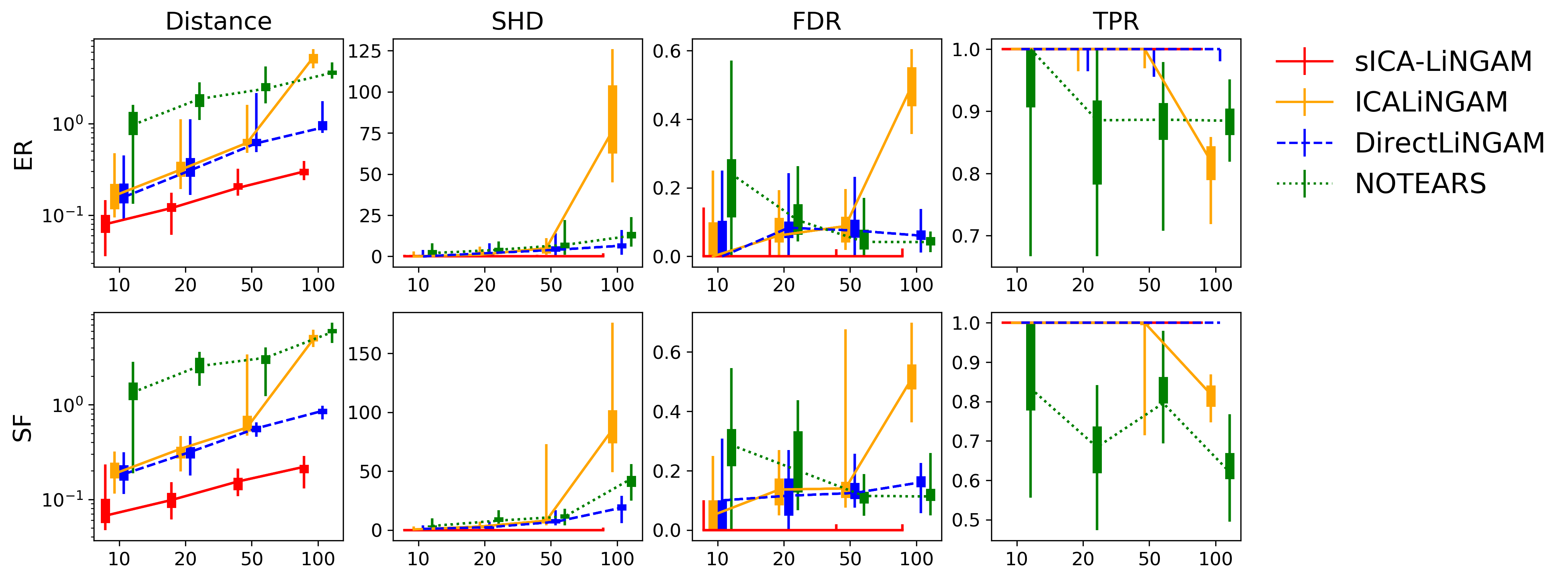
Figure 1: Four evaluation measures (Distance, SHD, FDR, TPR) over two graph types (ER, SF) and four graph sizes (10, 20, 50, 100). The x-axis is the graph size, and the y-axis is the value of each measure. The main line indicates the median of 20 simulations. The thick error bar and the thin error bar are the interquartile range and min-max range, respectively.

Post-Processing

We obtain the estimate $\hat{\mathbf{W}}$ from the optimization problem (20). However, we cannot estimate $\mathbf{B}$ directly via the relation $\hat{\mathbf{B}}=\mathbf{I}-\hat{\mathbf{M}}$ because of two problems, which are already described: (i) rows of $\hat{\mathbf{M}}$ have to be rearranged and rescaled so that all diagonal entries are one, and (ii) the estimate $\hat{\mathbf{B}}$ may not be acyclic, even if the true $\mathbf{B}$ is acyclic. These problems can be resolved by the method proposed in Shimizu et al. (2006). Here, we only show the outline of this method.

The problem (i) is resolved as follows. First, in order to obtain the matrix with non-zero diagonal entries, we search for a row permutation $\pi$ minimizing $\sum_{j=1}^{d}1/|\{\pi(\hat{\mathbf{M}})\}_{jj}|$. Next, we rescale the diagonal entries of $\pi(\hat{\mathbf{M}})$ to be one and divide each row by the same scale.

The problem (ii) is resolved as follows. To ensure the acyclicity, we repeatedly apply a test-and-cutoff procedure:

1. Test whether $\hat{\mathbf{B}}$ is acyclic or not.

2. If $\hat{\mathbf{B}}$ is not acyclic, replace the non-zero smallest absolute value of $\hat{\mathbf{B}}$ to 0, and return to step 1.

For the test of acyclicity, an efficient algorithm was proposed by Shimizu et al. (2006).

There is an additional device in the proposed method. After $\hat{\mathbf{B}}$ is made acyclic, the cutoff value is obtained. When this value is larger than pre-specified criteria $\omega_{1}(>0)$, such as $\omega_{1}=0.05$, we improve the estimate by increasing $\alpha$ and again estimating $\hat{\mathbf{M}}$ until $\hat{\mathbf{B}}$ is made acyclic with a smaller cutoff than $\omega_{1}$. This truncation seems ad-hoc, but relevant methods like NOTEARS set larger criteria like $\omega_{1}=0.3$. The proposed method worked well with much smaller cutoffs in numerical experiments, as shown in Figure 2. Furthermore, we can reduce false discovery of directed edges by additional cutoff $\omega_{2}>0$ for which the entries of $\hat{\mathbf{B}}$ is truncated to 0 if their absolute values are smaller than $\omega_{2}$.

Experiments

In this section, we show the performance of the proposed method by numerical experiments. On synthetic data, the proposed method (sICA-LiNGAM) was compared with ICA-LiNGAM, DirectLiNGAM, and NOTEARS. We did not include Pairwise LiNGAM, High-dimensional LiNGAM, and the method of Zhang et al. (2009) because the first two methods would show similar performances to DirectLiNGAM in our setting, as seen in Hyvärinen and Smith (2013) and Wang and Drton (2020), and the last method is considered to be unstable as discussed before. The scalability of the proposed method was examined in high dimensional data up to $d=500$ with a fixed sample size. The application to the real data was also conducted.

Comparison of the methods (by simulation)

Numerical experiments were conducted on synthetic data. We basically mimic the simulation settings of Shimizu et al. (2011) and Zheng et al. (2018). The linear DAG model with non-Gaussian noises was employed to generate observed variables. True graphs were generated from Erdös-Rényi (ER; Erdös and Rényi 1959) or Scale-Free (SF; Barabási and Albert 1999) models of different sizes ($d=10,20,50,100$), with the expected number of edges $d$. The weight parameters of a generated graph were uniformly drawn from the interval $[-1.5,-0.5]\cup[0.5,1.5]$. (The true non-zero weight parameters were avoided to be around zero.) The distribution of each noise was randomly selected from three non-Gaussian distributions (Laplace, uniform, and exponential). The noise variances were uniformly drawn from the interval $[1,3]$. We generated 20 datasets with a sample size of $N=1,000$. The noises were randomly drawn from the selected distributions.

The models were estimated by the proposed method, ICA-LiNGAM, DirectLiNGAM, and NOTEARS. We describe the settings for these methods. For the proposed method, the tuning parameter $\lambda$ was set to $\lambda=0.1$ throughout the experiments. The tuning parameter $\alpha$ was basically selected by 10-fold CV out of 50 points in the range $[10^{-3},10^{-0.5}]$ with a log scale. The initial estimate $(m_{jk}^{0})$ was estimated by the proposed method with $\gamma=0$, $\alpha=0$ for $d<50$, and $\alpha=0.1$ for $d\geq 50$. The step size was set at $\eta=0.005$. If the resulting estimate $\hat{\mathbf{B}}$ was not acyclic, the tuning parameter $\alpha$ increased until $\hat{\mathbf{B}}$ became acyclic. The two cutoff parameters $\omega_{1}$ and $\omega_{2}$ were both set at 0.05. Two stopping criteria for parameter updates were set to $\max{|\mathbf{W}_{t}\mathbf{D}^{-1}\mathbf{V}^{T}-\mathbf{M}_{t}|}<10^{-4}$ and $\max{|\mathbf{W}_{t+1}-\mathbf{W}_{t}|}<10^{-5}$. The proposed method was implemented in Python 3.6.8. For other methods, the authors’ implementations were used .

The methods were evaluated in terms of estimation error based on the Frobenius norm between the estimated and true weight matrices (Distance), Structural Hamming Distance (SHD), False Discovery Rate (FDR) and True Positive Rate (TPR). The metrics are detailed in the supplementary material. Figure 1 shows the main results. The proposed method achieved the best performances among all of the methods. This result was probably because the proposed method estimates the causal order and parameters simultaneously via the log-likelihood optimization with sparsity. This means the proposed method used all the information throughout the estimation process. The proposed method succeeded in improving ICA-LiNGAM by virtue of sparsity and, in particular, largely improved in the high dimensional setting $(d=100)$. NOTEARS was behind the others. It would be because the synthetic data did not satisfy the equal variance assumption, which seems necessary for NOTEARS.

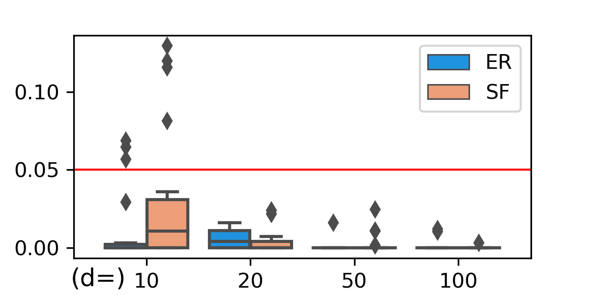
Figure 2: Cutoff values necessary to make $\hat{\mathbf{B}}$ acyclic at CV-selected $\alpha$. If the cutoff exceeded the criteria (red line), we increased $\alpha$.

Figure 2 shows the actual cutoff values necessary to make $\hat{\mathbf{B}}$ acyclic at CV-selected $\alpha$. Although we used $\omega_{1}=0.05$, the estimate $\hat{\mathbf{B}}$ could be acyclic with much smaller cutoff values in most cases. This indicates that we can estimate the acyclic graph in a much less ad-hoc manner.

Scalability of the proposed method

The scalability of the proposed method was examined in simpler and higher dimensional settings. The graphs were generated from the ER model with $d=100,200,500$, and noises were drawn only from the Laplace distribution. The expected number of directed edges was 50 or 100. The sample size and the other settings were the same as before. We evaluated the estimation error and computational time of the proposed method and DirectLiNGAM because these methods performed well for $d=100$ in the previous experiment. In order to evaluate the computational time conveniently, $\alpha$ of the proposed methods was fixed at 0.1. The experiments were conducted with a single 3.6 GHz Intel Core i7 CPU and a 32GB memory.

The results of 10 simulations are shown in Figure 3. Our method performed well, even in high dimensional settings. On the contrary, the estimate of DirectLiNGAM was unstable when $d=500$. Both methods finished in realistic computational times.

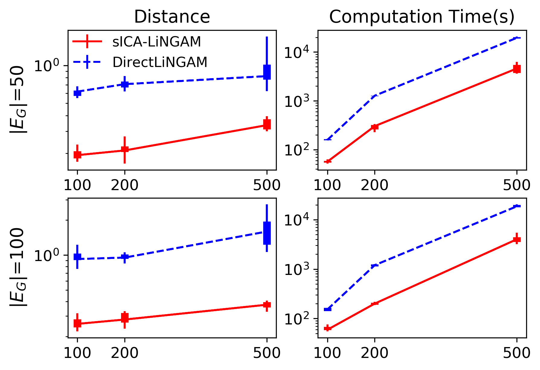
Figure 3: Estimation error and computation time based on 10 simulations. The x-axis is the dimension of the data.

Real Data

As described in Shimizu et al. (2006), a time series can be approximated by a linear DAG model, especially if the time series is a stationary AR(1). For example, when a time series is sliced into time windows with three time points, the AR(1) structure can be approximated by the linear DAG model of

$$\left\{\begin{array}[]{cl}X_{1}&=\varepsilon_{1}\\ X_{2}&=b_{21}X_{1}+\varepsilon_{2}\\ X_{3}&=b_{32}X_{2}+\varepsilon_{3}\end{array}\right..$$ (40)

Therefore, if the noises are independent and non-Gaussian, LiNGAM can express the AR(1) structure, and then recover the correct order from sliced time series.

We applied the same four methods to the Beijing Multi-Site Air-Quality Data (Zhang et al. 2017). This data includes hourly concentration measures of major air pollutants, such as nitrogen dioxide ($\mathrm{NO}_{2}$) and sulfur dioxide ($\mathrm{SO}_{2}$), recorded at national monitoring sites in Beijing. Each site provides every pollutant’s time series from March 1st, 2013 to February 28th, 2017. Each time series was sliced into 1,461 time windows with 24 time points so that each window consists of hourly measures of one day. The values were transformed by the function $\log(1+x)$. When a time window contained missing values, the window was removed. Every method was evaluated by a heatmap visualizing $\hat{\mathbf{B}}$. Suppose the AR(1) structure is recovered by the linear DAG model, only the $(j+1,j)$th cell is colored for $j=1,...,23$, and the other cells are not colored. Note that the proposed method used the CV-selected $\alpha$ because it was difficult to obtain the acyclic estimates by increasing $\alpha$.

Figure 4 shows the results on the data of Tiantan station. The proposed method succeeded in recovering the AR(1) structure very well, and non-AR(1) cells were almost shrunk to zero. ICA-LiNGAM also recovered the structure, but some non-AR(1) cells had non-zero values. By virtue of sparsity, the proposed method shrunk the small non-zero estimates of non-AR(1) cells to zero, and recovered the AR(1) structure better than ICA-LiNGAM. DirectLiNGAM and NOTEARS failed to recover about or more than half of the AR(1) structure. As seen in the supplementary material, the proposed method also showed the best performance clearly at the other monitoring sites.

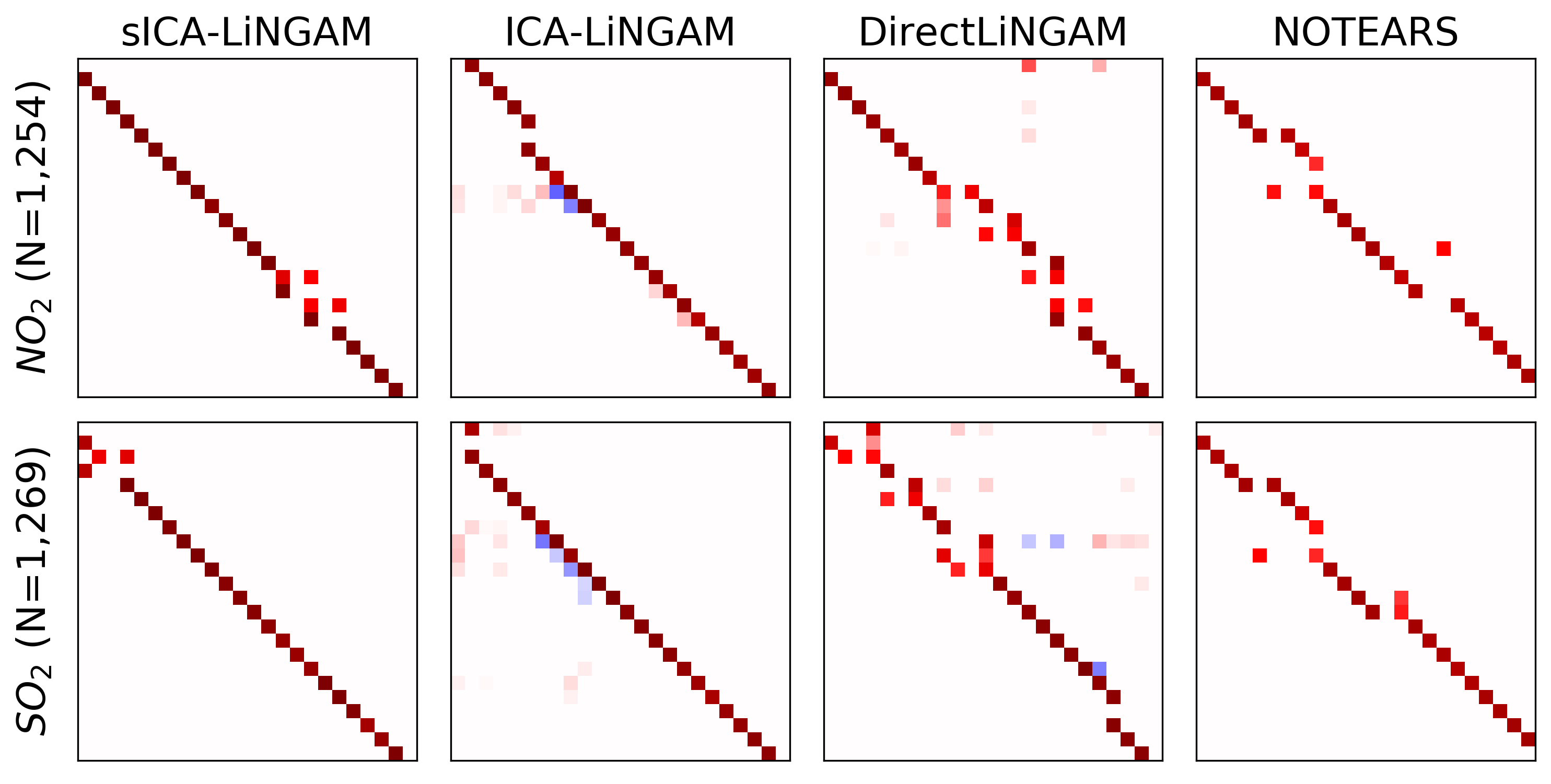
Figure 4: Heatmaps of $\hat{\mathbf{B}}$s at Tiantan station. Red/Blue indicates a positive/negative value. If the AR(1) structure is recovered correctly, the $(j+1,j)$th cell is colored for $j=1,...,23$ and the other cells are not colored.

Conclusion

In this paper, we have proposed a new estimating algorithm for a linear DAG model with non-Gaussian noises. The proposed method is based on the penalized log-likelihood of ICA, and estimates the causal structure and the parameter values at once. Several devices for a stable and efficient learning are introduced such as a penalty on orthogonality of the parameter matrix and a modified natural gradient. The proposed method achieved the best performance among the existing methods in the numerical experiments. Note that the norm constraints on the rows of $\mathbf{W}$ may not look necessary, but in our experience, the method without the constraint sometimes yielded an incorrect solution. For future works, it is significant to extend the method to non-DAG structures, such as data with cyclic structures and/or latent confounders.

Supplementary Information

Definitions of Evaluation Measures

We evaluated the estimates $\hat{\mathbf{B}}$ and the corresponding graphs by four metrics: 1) Distance, 2) Structural Hamming Distance (SHD), 3) False Discovery Rate (FDR), 4) True Positive Rate (TPR). The Distance is a measure for the estimation error. The other three measures are employed to evaluate the performance of causal discovery.

• Distance (Frobenius Norm of the Difference Between Two Matrices) : Distance is defined as the Frobenius norm of the difference between two matrices. The Distance between the estimate and the truth is evaluated:

  $$Distance=\|\mathbf{\hat{\mathbf{B}}-\mathbf{B}_{true}}\|_{F}.$$ (41)

• Structured Hamming Distance (SHD): SHD indicates the number of steps to transform the estimated graph into the true graph. The steps include edge additions, deletions, and reversals.

• False Discovery Rate (FDR): FDR is the proportion of false positives and reversed edges over the estimated edges.

• True Positive Rate (TPR): TPR is the proportion of true positive edges over the true edges.

Results of AR(1) Recovery at the Other Sites

We estimated $\hat{\mathbf{B}}$ by four methods (sICA-LiNGAM (proposed), ICA-LiNGAM, DirectLiNGAM, NOTEARS) at the three additional sites. If the AR(1) structure is recovered by the linear DAG model, only the $(j+1,j)$th cell is colored for $j=1,...,23$, and the other cells are not colored.

• At Aotizhongxin station (Figure S.1), the proposed method successfully recovered the time series especially on $\mathrm{SO}_{2}$. ICA-LiNGAM partly recovered the structure, but some non-AR(1) cells had non-zero values. DirectLiNGAM also recovered the structure on $\mathrm{NO}_{2}$, but failed to recover about two third of the AR(1) structure on $\mathrm{SO}_{2}$. NOTEARS failed to recover about or more than half of the AR(1) structure.

• At Nongzhanguan station (Figure S.2), the proposed method completely recovered the AR(1) structure except for the points of (1,24) and (21,22) on $\mathrm{SO}_{2}$. None of the other methods could recovered the AR(1) sequence successfully.

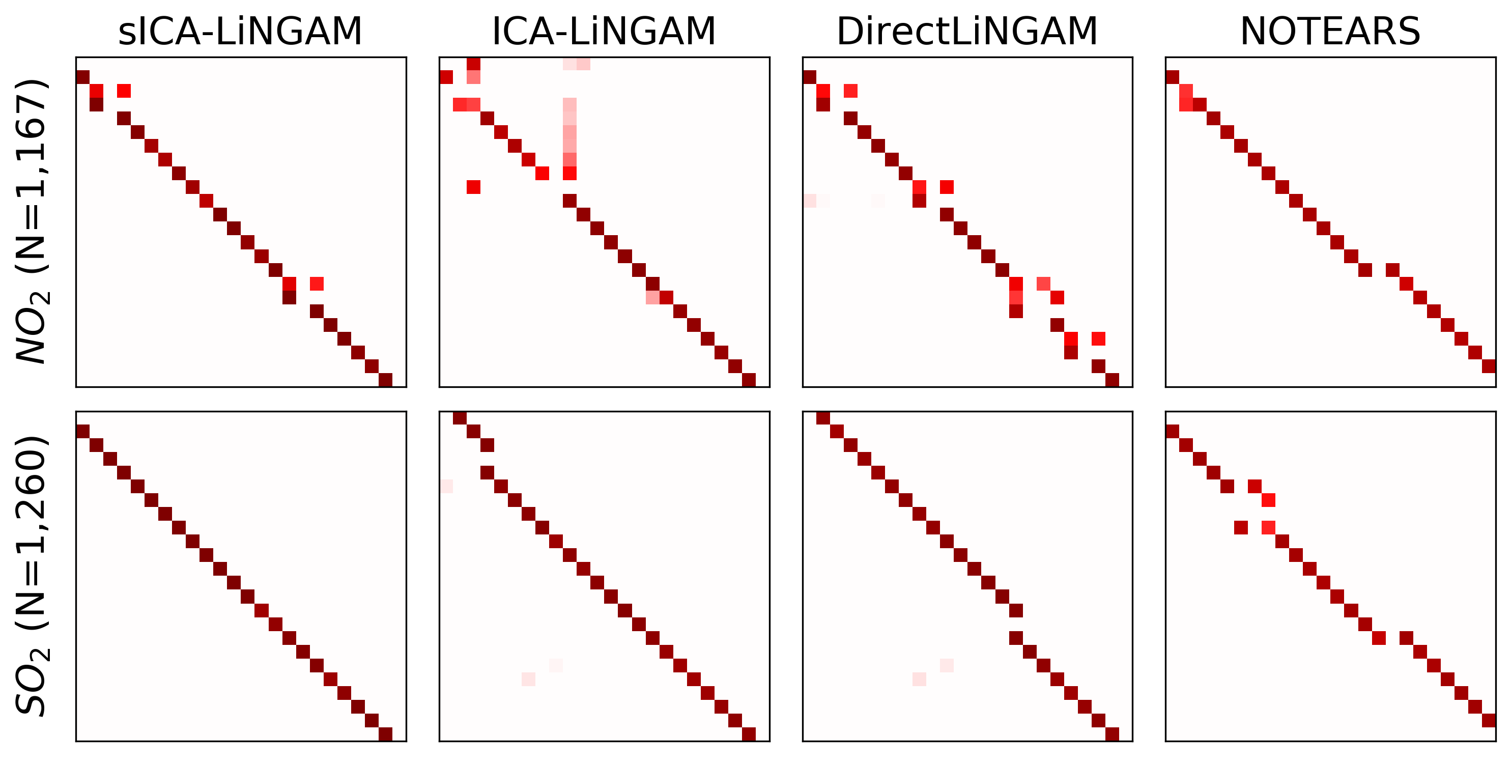
Figure S.1: Heatmaps of $\hat{\mathbf{B}}$s at Aotizhongxin station. Red/Blue indicates a positive/negative value.

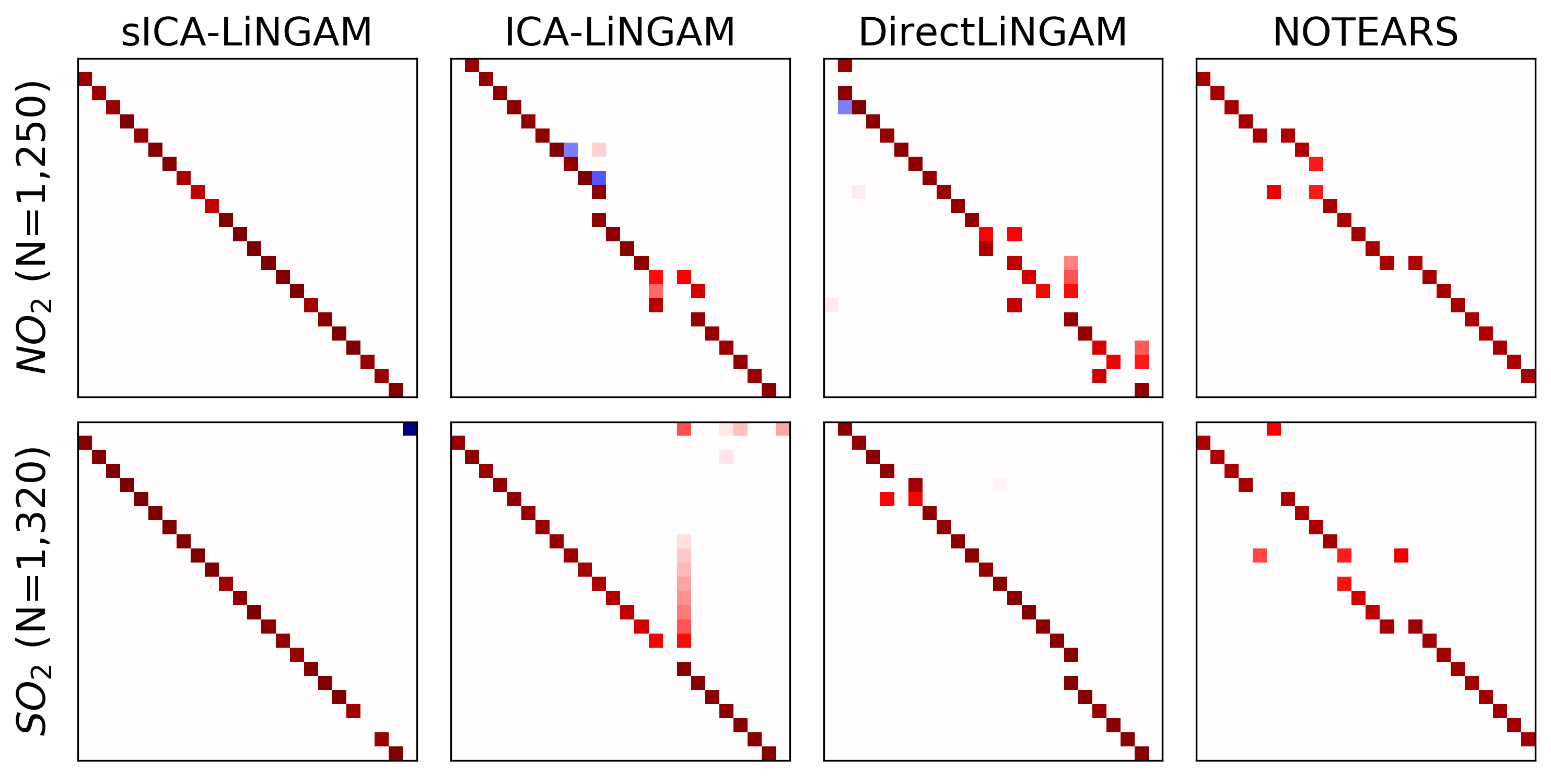
Figure S.2: Heatmaps of $\hat{\mathbf{B}}$s at Nongzhanguan station. Red/Blue indicates a positive/negative value.

References

- Amari (1998) Amari, S.-I. 1998. Natural Gradient Works Efficiently in Learning. Neural Computation 10(2): 251–276.
- Barabási and Albert (1999) Barabási, A.-L.; and Albert, R. 1999. Emergence of Scaling in Random Networks. Science 286(5439): 509–512.
- Bollen (1989) Bollen, K. A. 1989. Structural Equations with Latent Variables. John Wiley & Sons.
- Boyd, Parikh, and Chu (2011) Boyd, S.; Parikh, N.; and Chu, E. 2011. Distributed Optimization and Statistical Learning via the Alternating Direction Method of Multipliers. Now Publishers Inc.
- Chickering (2002) Chickering, D. M. 2002. Optimal Structure Identification with Greedy Search. Journal of Machine Learning Research 3(Nov): 507–554.
- Erdös and Rényi (1959) Erdös, P.; and Rényi, A. 1959. On Random Graphs I. Publ. Math. Debrecen 6(290-297): 18.
- Glymour (1998) Glymour, C. 1998. Learning Causes: Psychological Explanations of Causal Explanation. Minds and Machines 8(1): 39–60.
- Hastie, Tibshirani, and Wainwright (2015) Hastie, T.; Tibshirani, R.; and Wainwright, M. 2015. Statistical Learning with Sparsity: the Lasso and Generalizations. CRC press.
- Hoover (2008) Hoover, K. D. 2008. Causality in Economics and Econometrics. The new Palgrave Dictionary of Economics 2.
- Hyvärinen (1999) Hyvärinen, A. 1999. Fast and Robust Fixed-Point Algorithms for Independent Component Analysis. IEEE Transactions on Neural Networks 10(3): 626–634.
- Hyvärinen, Karhunen, and Oja (2001) Hyvärinen, A.; Karhunen, J.; and Oja, E. 2001. Independent Component Analysis. John Wiley & Sons.
- Hyvärinen and Smith (2013) Hyvärinen, A.; and Smith, S. M. 2013. Pairwise Likelihood Ratios for Estimation of Non-Gaussian Structural Equation Models. Journal of Machine Learning Research 14(Jan): 111–152.
- Hyvärinen et al. (2010) Hyvärinen, A.; Zhang, K.; Shimizu, S.; and Hoyer, P. O. 2010. Estimation of a Structural Vector Autoregression Model Using Non-Gaussianity. Journal of Machine Learning Research 11(5).
- Jolliffe, Trendafilov, and Uddin (2003) Jolliffe, I. T.; Trendafilov, N. T.; and Uddin, M. 2003. A Modified Principal Component Technique Based on the LASSO. Journal of Computational and Graphical Statistics 12(3): 531–547.
- Judea (2000) Judea, P. 2000. Causality: Models, Reasoning, and Inference. Cambridge University Press. ISBN 0 521(77362): 8.
- Liu et al. (2015) Liu, Y.; Wu, X.; Zhang, J.; Guo, X.; Long, Z.; and Yao, L. 2015. Altered Effective Connectivity Model in the Default Mode Network Between Bipolar and Unipolar Depression Based on Resting-State fMRI. Journal of Affective Disorders 182: 8–17.
- Peters and Bühlmann (2014) Peters, J.; and Bühlmann, P. 2014. Identifiability of Gaussian Structural Equation Models with Equal Error Variances. Biometrika 101(1): 219–228.
- Peters et al. (2014) Peters, J.; Mooij, J. M.; Janzing, D.; and Schölkopf, B. 2014. Causal Discovery with Continuous Additive Noise Models. The Journal of Machine Learning Research 15(1): 2009–2053.
- Sachs et al. (2005) Sachs, K.; Perez, O.; Pe’er, D.; Lauffenburger, D. A.; and Nolan, G. P. 2005. Causal Protein-Signaling Networks Derived from Multiparameter Single-Cell Data. Science 308(5721): 523–529.
- Shimizu et al. (2006) Shimizu, S.; Hoyer, P. O.; Hyvärinen, A.; and Kerminen, A. 2006. A Linear Non-Gaussian Acyclic Model for Causal Discovery. Journal of Machine Learning Research 7(Oct): 2003–2030.
- Shimizu et al. (2011) Shimizu, S.; Inazumi, T.; Sogawa, Y.; Hyvärinen, A.; Kawahara, Y.; Washio, T.; Hoyer, P. O.; and Bollen, K. 2011. DirectLiNGAM: A Direct Method for Learning a Linear Non-Gaussian Structural Equation Model. The Journal of Machine Learning Research 12: 1225–1248.
- Spirtes et al. (2000) Spirtes, P.; Glymour, C. N.; Scheines, R.; and Heckerman, D. 2000. Causation, Prediction, and Search. MIT press.
- Tibshirani (1996) Tibshirani, R. 1996. Regression Shrinkage and Selection via the Lasso. Journal of the Royal Statistical Society: Series B (Methodological) 58(1): 267–288.
- von Eye and DeShon (2012) von Eye, A.; and DeShon, R. P. 2012. Directional Dependence in Developmental Research. International Journal of Behavioral Development 36(4): 303–312.
- Wang and Drton (2020) Wang, Y. S.; and Drton, M. 2020. High-Dimensional Causal Discovery Under non-Gaussianity. Biometrika 107(1): 41–59.
- Wiedermann and Von Eye (2016) Wiedermann, W.; and Von Eye, A. 2016. Statistics and Causality. John Wiley & Sons.
- Xu (2017) Xu, X. 2017. Contemporaneous Causal Orderings of US Corn Cash Prices Through Directed Acyclic Graphs. Empirical Economics 52(2): 731–758.
- Zhang and Chan (2006) Zhang, K.; and Chan, L.-W. 2006. ICA with Sparse Connections. In International Conference on Intelligent Data Engineering and Automated Learning, 530–537. Springer.
- Zhang and Hyvärinen (2009) Zhang, K.; and Hyvärinen, A. 2009. On the Identifiability of the Post-Nonlinear Causal Model. In 25th Conference on Uncertainty in Artificial Intelligence (UAI 2009), 647–655. AUAI Press.
- Zhang et al. (2009) Zhang, K.; Peng, H.; Chan, L.; and Hyvärinen, A. 2009. ICA with Sparse Connections: Revisited. In International Conference on Independent Component Analysis and Signal Separation, 195–202. Springer.
- Zhang et al. (2017) Zhang, S.; Guo, B.; Dong, A.; He, J.; Xu, Z.; and Chen, S. X. 2017. Cautionary Tales on Air-Quality Improvement in Beijing. Proceedings of the Royal Society A: Mathematical, Physical and Engineering Sciences 473(2205): 20170457.
- Zheng et al. (2018) Zheng, X.; Aragam, B.; Ravikumar, P. K.; and Xing, E. P. 2018. DAGs with NO TEARS: Continuous Optimization for Structure Learning. In Advances in Neural Information Processing Systems, 9472–9483.
- Zou (2006) Zou, H. 2006. The Adaptive Lasso and Its Oracle Properties. Journal of the American Statistical Association 101(476): 1418–1429.
- Zou, Hastie, and Tibshirani (2006) Zou, H.; Hastie, T.; and Tibshirani, R. 2006. Sparse Principal Component Analysis. Journal of Computational and Graphical Statistics 15(2): 265–286.