Ray Tracing Structured AMR Data Using ExaBricks

Abstract

Structured Adaptive Mesh Refinement (Structured AMR) enables simulations to adapt the domain resolution to save computation and storage, and has become one of the dominant data representations used by scientific simulations; however, efficiently rendering such data remains a challenge. We present an efficient approach for volume- and iso-surface ray tracing of Structured AMR data on GPU-equipped workstations, using a combination of two different data structures. Together, these data structures allow a ray tracing based renderer to quickly determine which segments along the ray need to be integrated and at what frequency, while also providing quick access to all data values required for a smooth sample reconstruction kernel. Our method makes use of the RTX ray tracing hardware for surface rendering, ray marching, space skipping, and adaptive sampling; and allows for interactive changes to the transfer function and implicit iso-surfacing thresholds. We demonstrate that our method achieves high performance with little memory overhead, enabling interactive high quality rendering of complex AMR data sets on individual GPU workstations.

Introduction

1 Introduction

In many large-scale simulations performed today, the features being simulated are quite small relative to the computational domain. For example, the turbulent vortices formed through airflow over an airplane can be centimeters in size, but are the product of complex interactions between the air and geometry over the scale of the entire system (Ray Tracing Structured AMR Data Using ExaBricks). Other examples can be found in astrophysics, where scientists are interested in planetary-scale forces interacting over light-years of space; or in engineering, where millimeter-scale combustion effects are simulated in the context of a 20-story boiler.

To account for these massive spatial differences, modern simulation codes employ Adaptive Mesh Refinement (AMR) [8, 7, 12, 19, 15, 14, 31]: As the simulation progresses, an initially coarse grid is adaptively refined to preserve fine details. The output of such simulations are data sets containing significant differences in spatial resolution across the computational domain. For example, the ratio of largest to smallest cell size in the NASA Landing Gear data set is 4096 to 1 (Figure 9).

Although AMR has become increasingly common in simulations, visualizing the resulting data continues to pose a number of challenges. First, different simulation codes use different techniques for refinement, resulting in a number of different forms of AMR that a visualization pipeline must support. Moreover, for cell-centered AMR, artifact-free rendering requires a method of reconstructing a continuous scalar field from the discrete samples. As AMR data is inherently irregular, computing such samples requires non-trivial (and costly) operations such as tree traversals to query cell values.

Especially when reconstructing this scalar field across boundaries between different resolution levels, such methods are neither trivial nor cheap. As a result, current visualization approaches either significantly reduce the number of samples taken to achieve interactive rendering, sacrificing quality, or must take many expensive samples to achieve high-quality, sacrificing performance.

In this paper, we present a holistic approach to address the above issues. The core idea of our approach is to use a combination of three different but inter-operating data structures that address different parts of the problem: First, we avoid looking at individual cells, deep AMR hierarchies, octrees, etc; and instead re-arrange the data into a set of bricks, similar to previous approaches that reorganized the data or built additional hierarchies [17, 37, 40]. Second, on top of these bricks we build an additional spatial partitioning that is particularly designed for the AMR basis reconstruction filter [37] that stores for each region which bricks can influence the region. The regions can then be used for fast basis reconstruction during rendering without costly cell location kernels, along with space skipping and adaptive sampling. Third, we build an RTX BVH over the resulting regions, and use this for hardware-accelerated ray marching, space skipping, and adaptive sampling, while also supporting interactive transfer function and iso-surface editing.

Our approach supports interactive high-quality direct volume rendering with a smooth AMR reconstruction filter and gradient-based volume shading, combined with surface shading from implicit iso-surfaces and/or polygonal surfaces defined throughout the volume. In particular, our adaptive sampling approach guarantees that the sampling frequency can adapt to the finest level cell size while keeping total sample counts tractable. When combined with our fast sample reconstruction and RTX-accelerated ray marching, this allows for interactive visualization on individual GPU workstations, even for highly complex models. Our key contributions are:

• A data structure to reorganize AMR data that supports high-quality cell interpolation, including across level boundaries;

• A novel method to compute gradient vectors from just the samples taken for reconstruction;

• An adaptive sampling and opacity correction method for adaptive sampling of AMR data; and

• A thorough evaluation on realistic models and rendering methods.

2 Related Work

AMR data sets topologically resemble hierarchies of structured grids that store scalar fields, lending themselves to the typical rendering modalities for this type of data, namely, direct volume or iso-surface rendering. For the latter, Weber et al. [43, 42] proposed a scheme that extracts crack-free iso-surfaces from AMR data by first computing the dual mesh using unstructured mesh elements, and then extracting an iso-surface from the unstructured mesh [43]. Moran and Ellsworth [27] improved upon Weber et al.’s approach by constructing a more general dual-mesh that also works for data sets in which bricks at level boundaries can differ by more than one level.

(a)

(b)

(c)

(d)

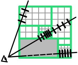
(e)

Figure 1: An illustration of our method for the simpler case of a nearest-neighbor reconstruction filter: (a) Given an input AMR data set, (b) we first extract the finest level cells in each region, discarding the original hierarchy. (c) We re-organize the cells into bricks containing grids of same-level cells, then for each of the green regions compute meta-information for adaptive sampling and space skipping, and construct an RTX BVH over these regions. (d) During rendering we traverse rays through the bricks, skipping those that are transparent. (e) Within each region we adapt the sampling rate to the corresponding cell size. When employing a smooth reconstruction filter, both the brick generation (a-c) and rendering (d, e) steps are the same; however, the Active Brick Regions are traversed instead of the bricks.

An alternative to extracting iso-surfaces is direct volume rendering (DVR) [22, 9, 33, 4]. Although DVR is widely used for regular structured grids, in particular on the GPU where hardware texture units can be leveraged for interpolation, DVR for AMR volumes is far more challenging. Weber et al. [43] proposed a method that first generated unstructured elements to stitch across level boundaries and then performed a scan conversion on these elements using the GPU. Park et al. [32] proposed a splatting approach, building off the cell projection method of Max [26]. Ma [25] also proposed a ray tracing approach, but assumed that cell-centered AMR could easily be converted to vertex-centered AMR, which in general is not the case at level boundaries.

More closely related to our method is the technique proposed by Kähler et al. [17]. As in our method, Kähler finds a tailored spatial partitioning with blocks that contain only same-level cells, discarding the original AMR grid hierarchy. Their approach uses a multi-pass rendering method, can leverage hardware-accelerated texture sampling on the GPU, and includes a form of adaptive sampling by adjusting the sampling rate within a block. Kähler and Abel [16] later extended this method to work in a single rendering pass by using bindless textures and traversing the $k$-d tree in the fragment shader, though the multipass method was found to perform best. However, their method only works for either nearest reconstruction or vertex-centered AMR, and does not support smooth reconstruction at all for the cell-centered AMR that most current simulations use.

For rendering Octree AMR data, Labadens et al. [20] proposed using the octree to generate volume splats, or traced rays through the octree to perform volume integration at the leaves. However, their approach also supports only nearest neighbor interpolation.

Along with iso-surface extraction, Moran and Ellsworth’s [27] unstructured dual-mesh framework is also capable of high-quality volume rendering of AMR data. Their framework did not aim for interactive rendering, but produced high quality imagery and scaled to large models. To achieve high-quality volume rendering, Moran and Ellsworth introduced an adaptive sampling approach which adjusts the sampling rate to match the local data frequency.

To avoid the need to construct an unstructured dual-mesh or unstructured stitching elements, Wald et al. [37] and Wang et al. [41] proposed several reconstruction filters that can operate directly on the cell-centered AMR data. As with our presented work, these papers aimed at interactive rendering of AMR data within a ray tracing framework (in their case, OSPRay [38]), and support both direct volume and implicit iso-surface rendering. However, both methods still suffer from two main shortcomings. First, both require the frequent use of costly cell location kernels, making computing samples expensive. Second, they do not introduce any space skipping or adaptive sampling tailored for AMR data, and instead rely on OSPRay’s existing adaptive sampling code, which is not aware of the underlying AMR hierarchy and thus may severely under- or over-sample the data. In this paper, we adopt the basis interpolation method introduced in [37] to provide a continuous interpolant across level boundaries, but do not require the costly cell location kernels that limited the original method’s performance.

A key difference of our approach using the basis method compared to prior AMR rendering work by Leaf et al. [21] leveraging the multiresolution interblock interpolation of Ljung et al. [24], is that the basis function’s support is not truncated at the first sample on the neighboring side. Although this leads to a smoother interpolant, it also results in larger support overlap between cells from neighboring blocks.

Wang et al. [40] recently presented a reconstruction algorithm for high-quality rendering of Tree-Based AMR data, combined with a sparse octree representation for traversal. Their interpolant works by virtually introducing unstructured elements to stitch across boundaries, which fall into a fixed number of cases for which the interpolation weights can be precomputed. They achieve empty space skipping and adaptive sampling through their sparse octree. However, the large number of top-down octree traversals required for sample reconstruction in their approch impacts rendering performance.

With regard to empty space skipping, Ganter and Manzke [13] (for structured volumes) and Morrical et al. [28] (for unstructured volumes) proposed to leverage modern graphics hardware for on-the-fly space skipping through hardware-accelerated ray tracing. For unstructured data, Morrical et al. [28] further improve rendering performance by adapting the sampling rate to the data variation within regions of a spatial subdivision that they computed over the unstructured elements; they also used RTX capabilities for marching through these regions. In this work, we adopt a similar strategy for space skipping and adaptive sampling, but on top of our proposed data structure.

3 The ExaBricks Hierarchy

The core idea of our method is to use a combination of three different inter-operating data structures and associated algorithms to jointly address the different aspects of the problem to efficiently render AMR data with smooth interpolation.

First, we re-organize the input AMR cells into a set of compact, non-overlapping bricks of same-level cells, as proposed by Kähler et al. [17]. These bricks can be extremely small, e.g. on the Exajet bricks with 1, 2, or 4 cells are in fact quite common at level boundaries; however, in larger homogeneous regions these bricks allow for storing cells in a memory-efficient manner (Section 3.1).

Second, for each of these bricks we compute the region of space where the reconstruction filters associated with the brick’s cells are non-zero. When using a nearest reconstruction filter these regions are just the brick’s bounds; however, for any smooth interpolant these regions extend beyond the brick and result in overlapping regions of support (see Figure 3). We compute a second spatial partitioning structure over these support regions, the Active Brick Regions (ABRs), to produce a data structure where each leaf stores a list of the bricks that potentially influence the spatial region covered by the leaf. For any smooth interpolant, the resulting ABRs are more complex in shape and number than the original bricks. The ABRs are best seen as the “glue” of our method, that allow us to combine the bricks for low overhead storage (Section 3.1), smooth reconstruction filters and cell location without top-down queries (Section 3.2), space skipping (Section 4.1), and adaptive sampling (Section 4.2) into a single coherent method.

Finally, we build an RTX BVH over the ABRs that we use to quickly iterate over those that a given ray needs to integrate, while skipping those it is safe to ignore (Section 3.3).

3.1 Organizing Cells into Bricks

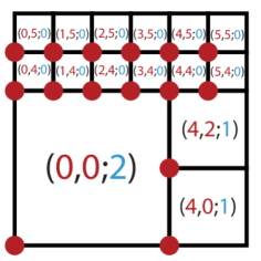
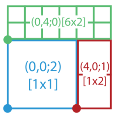
Figure 2: Cells and Bricks. Left: A 2D illustration of the input AMR cells showing 15 cells over three levels, labeled by their $(i,j;l)$ coordinates. Right: The bricks computed for these input cells, labeled by their $(i,j;l)$ coordinates and $[N\times M]$ dimensions.

The first stage of our method is to (re-)organize the input data set’s AMR cells into a set of bricks. Our definition and construction of these bricks is similar to that of Kähler et al. [17], and thus we focus on introducing the terminology required for the subsequent sections.

3.1.1 Cells

We adopt a terminology where level 0 is the finest level, with an implicit cell size of $1^{3}$, level 1 the next coarser level with cells of size $2^{3}$, level 2 coarser yet with cells of size $4^{3}$, and so on. This follows the terminology used by PowerFlow [11] and Cart3D [1], but is the reverse of others such as Chombo [8]. We can refer to any cell on a given level using four values, $(i,j,k;l)$, where $(i,j,k)$ are the lower-left unit coordinates of the cell and $l$ is its level. Each cell contains a single data value. Cells are arranged by the AMR simulation into blocks of grids in Block-Structured AMR layouts [3, 8] or an Octree in Tree-Based AMR layouts [1, 11].

Given the refinement rules outlined by Berger and Oliger [3], we know that $i,j,k$ are all multiples of $2^{l}$, and that cells will not overlap. Unlike Berger and Oliger’s constraints, we do not require cells to be fully refined (“holes” are explicitly allowed), nor do we require only single-level differences at level boundaries, making our method applicable to a wide range of different AMR refinement schemes. An illustration of the terminology we use is given in Figure 2.

3.1.2 Bricks

Similar to Kähler and Abel [16], we discard any AMR hierarchy information that is stored in the input data and reorganize the unordered list of cells into a set of non-overlapping bricks of same-level cells. The scalars for each brick are stored in a separate array, with a 3D array of scalars per-brick. This enables us to support a wide range of structured AMR data formats (e.g., Block-Structured, Octree, Cartesian). For each brick, we store the coordinates of the lower-left corner ($i,j,k$), the level ($l$), and the number of cells stored in each dimension ($N,M,K$) (see Figure 2).

To generate the bricks, we build a $k$-d tree whose leaf nodes contain only same-level cells. The tree is built top-down, and a leaf node created if all cells within the current node are on the same AMR level and completely fill their combined bounding box. To avoid bricks becoming so large as to not provide fine enough granularity for space skipping we limit leaves to be at most 32 cells wide on any axis. In contrast to Kähler and Abel, the children of an inner node are made by simply splitting the current cells along the longest axis of the node’s bounding box, which we found to provide better rendering performance. Split positions are rounded to an integer multiple of the current coarsest cell width to ensure cells are never split during the partitioning. We then discard the hierarchy and store only the resulting leaves, corresponding to the bricks.

3.2 Basis Method and Active Brick Regions

The bricks produced, per the previous section, are readily usable for rendering with a nearest-neighbor reconstruction filter, as illustrated in Figure 1 and described by Kähler and Abel [16]. However, nearest-neighbor reconstruction has obvious limitations in terms of image quality, in particular for spiky transfer functions and/or iso-surfaces. High-quality rendering requires the use of a more advanced reconstruction filter.

Due to its simplicity and ease of implementation, for this paper we chose to use the basis method by Wald et al. [37] for reconstruction. In this method, each cell $C$ of width $C_{w}$ is associated with a hat-shaped basis function:

$$\hat{H}_{C}(p)=\hat{h}\bigg{(}\frac{|C_{p_{x}}-p_{x}|}{C_{w}}\bigg{)}\hat{h}\bigg{(}\frac{|C_{p_{y}}-p_{y}|}{C_{w}}\bigg{)}\hat{h}\bigg{(}\frac{|C_{p_{z}}-p_{z}|}{C_{w}}\bigg{)},$$ (1)

where $\hat{h}(x)=\max(1-x,0)$. Reconstructing a sample at position $p$ then involves finding all cells $C_{i}$ with data value $C_{v_{i}}$ that have non-zero support $\hat{H}_{C_{i}}(p)$ and computing the weighted sum:

$$B(p)=\frac{\sum_{C_{i}}\hat{H}_{C_{i}}(p)C_{v_{i}}}{\sum_{C_{i}}\hat{H}_{C_{i}}(p)}.$$ (2)

3.2.1 Fast Basis-Method Sample Reconstruction

The problem that occurs when using any non-nearest reconstruction filter is that the reconstruction for a sample may—and typically will—be influenced by many different cells, potentially from different bricks at different AMR levels. To compute the reconstruction for a sample, Wald et al. [37] used a cell location kernel that would execute several recursive $k$-d tree traversals until all the required cells were found. This method is elegant, but costly even on a CPU with large caches. To avoid these per-sample $k$-d tree traversals we instead build a second data structure, the ABRs, that, for each region of space, tells us exactly which bricks can possibly influence that region. Thus, assuming one is in a leaf of this data structure, all that is required to perform a basis reconstruction is to iterate over the bricks referenced by this region, find the cells within each brick that influence the sample, and add their contributions. As each brick is a 3D grid, finding the required cells within the brick is trivial once the brick is known.

(a)

(b)

(c)

(d)

Figure 3: A 2D Illustration of our Active Brick Regions: (a) A data set with three bricks, each of a different refinement level. (b) The brick support regions corresponding to each brick. (c) The overlap of these supports forms a spatial partitioning where each region knows which bricks are “active” within it. (d) We subdivide these regions into non-overlapping rectangular regions which we can traverse as before.

3.2.2 Extending Bricks to Support Smooth Interpolation

To compute the ABRs to allow for smooth interpolation across level boundaries, we define the support of a cell $C$ as the region of space where $\hat{H}_{C}$ is non-zero. For the basis method, the support is a rectangular box extending exactly half a cell width beyond what is covered by $C$ itself. Similarly, we define the support of a brick $B$ as the union of the supports of that brick’s cells. Thus, a brick’s support is a box exactly half that brick’s cell width larger than the brick. The exact extent of the brick’s support depends on the level of its cells but, as each brick consists of cells on the same level, it is always a rectangular region (see Figure 3a and b).

We observe that the superposition of all brick supports forms a partition of space, where each region can be associated with exactly those bricks whose supports overlap in that region (see Figure 3(c)). These regions are formed by the intersection of the various brick supports, and are not necessarily rectangular or even convex. However, the edges of each region will be parallel to the coordinate axes, and thus they can be decomposed into the rectangular non-overlapping Active Brick Regions. Each ABR tells us exactly which bricks are “active” in that region of space, in the sense that at least one cell from these bricks has non-zero contribution in the region.

For each ABR, we store a list of the brick IDs active in the region and the bounding box of the region. We also compute and store additional meta-information about the region to enable empty space skipping and adaptive sampling. To enable empty space skipping, we compute the minimum and maximum scalar value of any cell whose support overlaps the region. As the basis method is a linear combination of the cells’ values, this range will also bound the value of any sample reconstructed in the region. We also store the cell width of the finest level that influences a region to later adapt the sampling rate for adaptive sampling.

3.2.3 Constructing the Active Brick Regions

To construct the active brick regions we again use a recursive top-down partitioning algorithm, similar to that used for building the bricks in Section 3.1. We begin by creating a list of “brick support fragments”, where each fragment specifies a box of space which it covers and the ID of the brick that is covered by it. The input list contains one fragment per brick, with each input fragment covering the brick’s entire support region. We then compute the bounding box of all the fragments, and begin a recursive subdivision.

In each subdivision step we need to consider a region to subdivide (initially, the entire bounding box), and a list of brick support fragments that overlap the region. To find a partitioning plane we iterate through the set of fragment boundaries and look at their respective faces, each of which defines a potential partitioning plane. From these, we select the one that is closest to the current region’s spatial center, preferably along the dimension where the region is widest. If no such plane exists in any dimension we know the current region does not contain a support boundary and can create a leaf with the current set of brick IDs. Otherwise, we partition the region into two subregions, sort the fragments overlapping the region into the left and right subtrees, and recursively partition the subtrees. The output leaves of this partitioning process are the active brick regions. We show statistics about the number of cells, bricks, and regions for a number of different AMR data sets in Table 1.

Each active brick region tracks the brick IDs that may influence the region, allowing us to eliminate the costly top down $k$-d tree traversals originally required for cell location in the basis method [37]. For each region we know exactly the bricks influencing it, and can quickly retrieve the required cells from the brick’s 3D array.

Table 1: The number of cells, bricks, and regions for each data set, and the average bricks/region, weighted by a simple average (by count) and by volume, to account for access probability.

				Avg. #Bricks/Region
Model	#Cells	#Bricks	#Regions	By Count	By Volume
Cloud	102M	528K	9M	3.46	1.09
Impact-5K	26.8M	515K	12.3M	3.42	1.24
Impact-20K	158M	3.4M	89.6M	3.46	1.75
Impact-46K	283M	3.1M	77.1M	3.45	1.74
Wind	411M	24.6K	689K	2.78	1.72
Gear	262M	26K	792K	2.97	1.20
Exajet	656M	3.1M	55.8M	3.18	1.25

3.3 BVH over Active Brick Regions

The active brick regions will allow each ray to know exactly which bricks influence a certain region of space and at what frequency; however, we still require a means of efficiently iterating a ray through the regions it intersects. One option to do so would be to store the split planes used during region construction—which form a $k$-d tree—and use this tree over the regions in the same manner that Kähler et al. [17] used their $k$-d tree over bricks. This approach would require implementing a software $k$-d tree traversal in a shader program with a per-thread stack and non-trivial control flow, similar to the single-pass approach of Kähler and Abel [16] but over our regions.

We instead leverage the new RTX hardware available on GPUs to enable hardware-accelerated traversal of the regions. To do so we discard the $k$-d tree produced by the region builder and store only the final regions. We then create an RTX user geometry with as many primitives as we have ABRs to construct an acceleration hierarchy over them. Our approach for rendering with the produced BVH is discussed in the following section.

4 Rendering with the ExaBricks Data Structure

Each ray that is traversed through the RTX BVH in hardware is first initialized with a search interval $[0..t_{\text{max}})$. If no region is found the ray has terminated; otherwise we compute the interval $[t_{\text{in}},t_{\text{out}}]$ that the ray overlaps with the intersected region, and volume-integrate this interval over the region as described below. To find the next ABR we trace another ray starting from $t_{\text{out}}+\mathcal{E}$ and repeat until the ray becomes opaque (for early ray termination), or no subsequent region is found.

Using a new ray traversal for each iteration step means that each volume ray will perform several hardware ray traversals. However, thanks to hardware support these rays are cheap, and can typically be amortized over multiple samples taken within the next region.

4.1 Space Skipping

In addition to amortizing the cost of taking multiple samples in the region, we also use the ABRs for space skipping. Truly empty space, i.e., areas outside the AMR mesh or holes in the mesh, will be automatically skipped as such areas do not generate bricks or regions. The more challenging case for space skipping are regions that are covered by cells whose visibility depends on the transfer function. During BVH construction we use each ABR’s precomputed scalar range to compute the maximum opacity of the transfer function within the range. If the maximum opacity for this range is 0, we know that every sample taken in this region would be fully transparent, and consequently that the entire region can be excluded from the BVH. Regions that are fully transparent are discarded during BVH construction by returning an empty box, those that are not simply return their bounding box.

In particular, we note that we do not have to construct any additional structure for space skipping (e.g., as done by Morrical et al. [28]), nor do we have to check a region’s validity during traversal. Inactive regions will never even be seen by any ray, as they are not even in the BVH being traversed.

The downside of this approach it that it requires updating the BVH each time the transfer function or iso-value changes. However, even on our largest data set (the Exajet), a full rebuild takes roughly 300ms on a Titan RTX or RTX 8000 GPU. This time could be further improved by refitting the BVH rather than rebuilding it.

4.2 Adaptive Sampling

Adaptive sampling is key to sampling the finest regions of an AMR data set at the same (relative) rate as the coarsest ones. For example, on the NASA Landing Gear the coarsest cells are 4096 times the size of the finest. Any technique that does not adapt the sampling rate by the same factor will either grossly over-sample coarse regions or under-sample fine ones.

To support adaptive sampling, we leverage each ABR’s metadata to adapt the sampling rate when traversing it to match the frequency of the data it contains. In contrast to Morrical et al. [28], we do not have to guess at the data frequency within a region, but can simply take the smallest cell size within the region. We then set a base sampling rate of two samples per smallest cell size in the region. The sampling rate can be scaled by a user-provided parameter to optionally subsample the data to trade quality for rendering performance. The examples shown in this paper use the high quality base sampling rate.

For each region we compute the first sample distance $t_{0}=dt(\rho+\lceil\frac{t0+\rho dt}{dt}\rceil)$, where $\rho$ is a per-ray random offset for interleaved sampling [18], and $dt$ is the scaled base sampling step. We then step the ray through the region, sampling at each $t_{i+1}=t_{i}+dt$. Our approach differs from the multi-block adaptive sampling proposed by Ljung [23] in that we do not define a global set of finest level samples that we skip according to the coarseness of the region. Instead, each region defines its own sampling intervals, independent of the others.

4.3 Opacity Correction

Figure 4: If successive regions are sampled at different rates, the distance between the last sample in one and the first sample in the next can be smaller (A) or larger (B) than either region’s sampling rate, leading to artifacts at region boundaries. We treat the sample points as delimiters which split the region’s overlap interval into sub-intervals (C). Each sub-interval is sampled at its mid-point and weighed by its length, ensuring samples are spaced as expected.

To account for the now variable step size between samples we use opacity correction [10], according to the term $\tilde{\alpha}=1-(1-\alpha)^{s/s_{1}}$, where $s$ is the current step size, $s_{1}$ is the base step size, and $\alpha$ is the opacity obtained from the transfer function.

However, even with this correction we encountered rendering artifacts at region boundaries. We root-caused these to the fact that the first and last samples from successive regions can lie closer together or further apart than the sample step size of the adjoining regions would suggest (Figure 4). To correct for this, we do not actually sample at the sample positions $t_{0},t_{1},...t_{n}$, but instead view them as delimiters for the intervals $T_{0}=[t_{in},t_{0}]$, $T_{1}=[t_{0},t_{1}]$, …, $T_{m}=[t_{n},t_{out}]$. We then sample each of these intervals in the middle $\left(\frac{T_{i}[0]+T_{i}[1]}{2}\right)$, and weigh it in the opacity correction term with the interval length, $dt_{i}=|T_{i}|$.

Compared to the adaptive sampling approach described above, this correction takes one additional sample from each region, and at least one sample for each region hit, even if the overlap interval is small. With our approach the opacity will not decrease due to undersampling, which can cause objectionable artifacts. Instead, at lower sampling rates biasing the sample positions results in some slight banding artifacts. Although both artifacts disappear in the limit with higher sampling rates, the artifacts—and in fact incorrect opacity—from undersampling regions are still very apparent at sampling rates where banding is only very faint or not visible at all (see Figure 5).

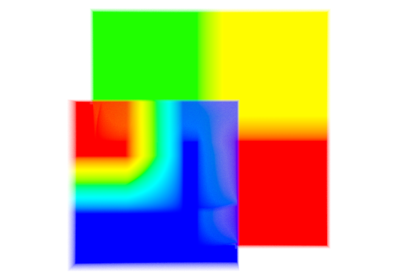
(a) w/o sample correction, $dt=0.3$

(b) w/ sample correction, $dt=0.3$

(c) w/o sample correction, $dt=2.0$

(d) w/ sample correction, $dt=2.0$

Figure 5: We correct sample positions so that each region is always sampled at least once. Without correction, at low sampling rates (base sample step $dt$), regions become translucent, while our sample correction manifests as less objectionable banding artifacts. Note that in the above images, the transfer function is fully opaque.

5 Implementation Details

We implement our method using OptiX 7 [34], though we note the same concepts are applicable to other GPU or CPU ray tracers. All rendering operations are implemented in a ray generation program, which performs both the iteration through the bricks as well as the integration within each region. All data is uploaded to CUDA memory buffers that this ray generation program operates on. Multi-GPU rendering is supported by simply replicating the data buffers on all GPUs, and assigning different GPUs to render different regions of the image.

5.1 Gradient Vectors

Local shading with a bidirectional reflectance distribution function (BRDF) requires gradient vectors to be computed as stand-ins for the nonexistent surface normals. A standard approach for computing these gradients is via central differencing at the sample point (Section 5.1.1) at the cost of additional samples. In our implementation, we employ an analytic gradient approach suitable for the basis reconstruction method that does not require additional samples (Section 5.1.2).

5.1.1 Central Differencing

We compare two ways of computing central difference gradients. Both require us to compute six additional basis reconstruction samples at positions offset from the current sample at a distance proportional to the current region’s sample rate. When sampling at the boundary of a region these offsets may require us to compute samples in other neighboring regions. We perform the cell location similar to Wald et al. [39], by tracing an infinitesimal ray originating at each offset position through the region BVH to find the containing region. Although the BVH traversal is hardware accelerated, this requires six additional rays to be traced per sample, incurring significant cost. To improve performance at the cost of quality, we also implemented a variant that clamps the offset positions to the current region before evaluating them, removing the need for additional ray traversals. We refer to this mode as clamped central differences. We observe that even with the accurate method, gradients are not necessarily continuous, as the offset size can change at level boundaries.

5.1.2 Analytic Gradients

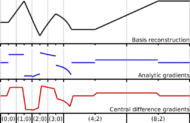
Figure 6: A 1D illustration of analytic vs. central difference gradients. Top: basis reconstruction with four level-0 and two level-2 cells. Middle: derivative of the reconstructed signal computed analytically from the same data values used for the reconstruction. Bottom: central differences require the signal to be reconstructed at additional positions to the left and right of the sample. Basis reconstruction is continuous, but not continuously differentiable, leading to shading artifacts at cell and level boundaries. Central difference derivatives are continuous but expensive to compute.

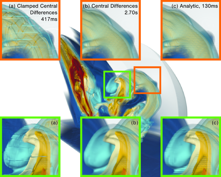
Figure 7: Different methods to compute gradients for shading, and rendering times obtained for the LANL Impact data set. (a) Clamped Central Differences: sample positions are clamped to remain within the region for performance, resulting in artifacts at region and level boundaries. (b) Central Differences: samples in neighboring regions required to compute the central difference are looked up through additional ray traversals. The resulting gradients are high-quality but prohibitively slow to compute. (c) Analytic: when computing the basis function contribution we determine the partial derivatives analytically using Equation 3. Analytic gradients are nearly as accurate as (b), but do not require additional data loads or ray traversal, and thus incur little performance impact.

For our third option to compute gradients, we observe that for the basis reconstruction method it is actually possible to compute the gradient analytically. This means that the gradient can be computed using just the existing data values loaded for the original sample evaluation, without additional memory accesses or ray traversals. The gradient can be computed as the first order partial derivatives of Equations 2 and 1 (shown only for $x$ below as an example):

$$\frac{\partial B(p)}{\partial x}=\frac{\sum_{C}\hat{H}_{C}(p)\sum_{C}\frac{\partial\hat{H}_{C}(p)}{\partial x}C_{v}-\sum_{C}\hat{H}_{C}(p)C_{v}\sum_{C}\frac{\partial\hat{H}_{C}(p)}{\partial x}}{(\sum_{C}\hat{H}_{C}(p))^{2}},$$ (3)

with

$$\frac{\partial\hat{H}_{C}(p)}{\partial x}=\hat{h}\bigg{(}\frac{|C_{p_{y}}-p_{y}|}{C_{w}}\bigg{)}\hat{h}\bigg{(}\frac{|C_{p_{z}}-p_{z}|}{C_{w}}\bigg{)}\chi(x)\frac{1}{C_{w}}$$

and

$$\chi(t)=\begin{cases}-1,&\text{if }C_{p_{t}}-p_{t}\geq 0\\ 1,&\text{otherwise}\end{cases}$$

Central differences will just connect neighboring point samples in an epsilon region and are thus guaranteed to be continuous. In comparison, the analytic gradient is arguably more “correct” but not always continuous (see Figure 6), which can lead to slightly worse image quality compared to central differences. However, analytic gradients provide far superior quality than clamped central differences and are much faster to compute than both central difference variants (Figure 7). Thus, they are used by default in our renderer.

5.2 Rendering Modes

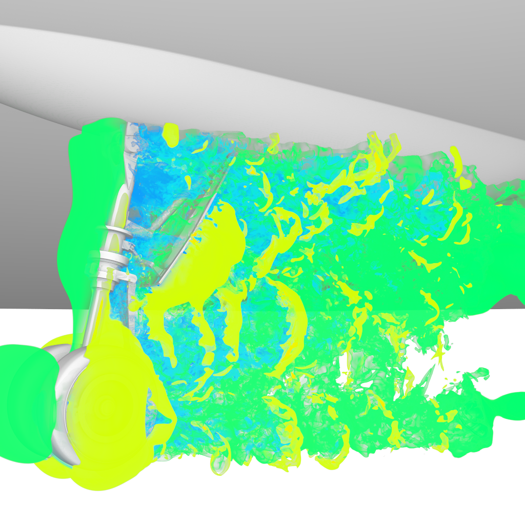
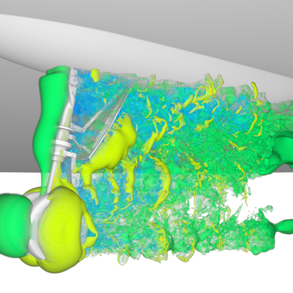
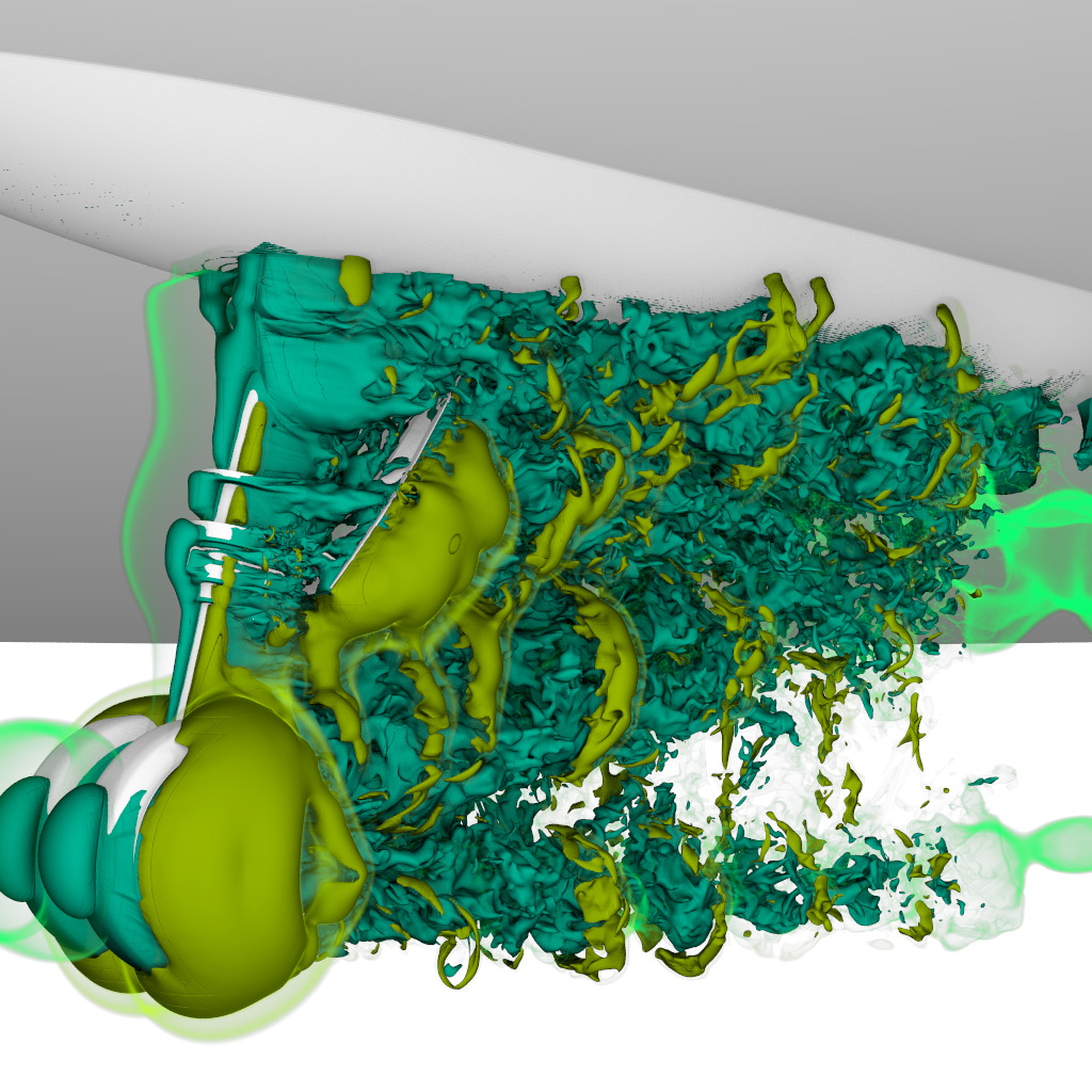
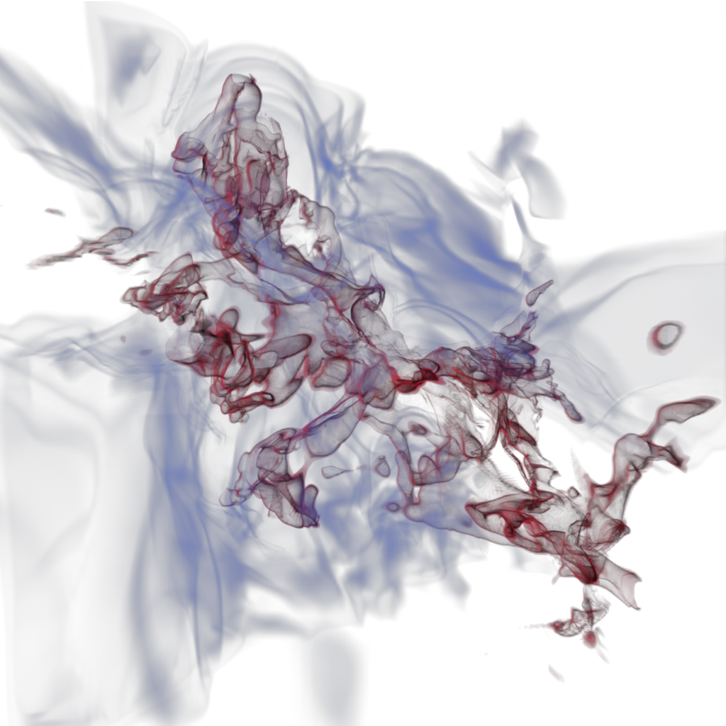
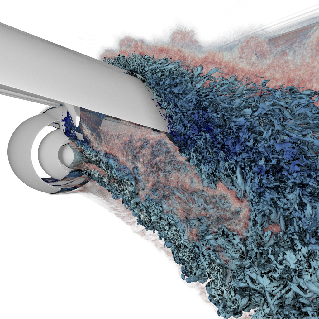
Figure 8: Examples of the rendering features in our framework. Top: the NASA Landing Gear with direct volume rendering only (left), gradient shading using analytic gradients (center), and with implicit iso-surface, volume rendering, and ambient occlusion (right). Bottom: Multi-field volume rendering of the TAC Molecular Cloud (left), and the Exajet with a triangle surface, color-mapped iso-surface, and volume, clipped to highlight interior features, with ambient occlusion.

We support a variety of different rendering modes to be able to evaluate our data structure under realistic conditions, including implicit iso-surfaces and direct volume rendering using ray marching. We maintain separate BVHs for volume data and iso-surfaces, as iso-surfaces in general have much more potential for empty space skipping due to their sparsity. As with the volume BVH, the iso-surface BVH must be rebuilt when the iso-value changes. We also support surface geometry represented as triangle meshes which are rendered using the RTX hardware-accelerated ray-triangle intersection test. We implement clipping planes by setting the rays’ [ray.tmin, ray.tmax] intervals accordingly (demonstrated on the Exajet in Figure 8 and the LANL Impact in Figure 9).

In the presence of iso-surfaces or meshes, we first trace each ray against the (fully hardware-accelerated) mesh BVH, then transform it into the volume space, and trace it against the iso-surface BVH to check for a closer surface hit point. We then shorten the ray to the nearest surface hit point, if any, and trace it through the volume BVH to integrate the volume up to that point. For better depth cues, we also support ambient occlusion rendering in addition to local shading.

Bricks and regions contain only spatial information about the cells, but can refer to more than one scalar field. We exploit this property to support color-mapping an iso-surface computed on one field with colors computed from another—for example, flow velocity mapped on to the vorticity iso-surface in Ray Tracing Structured AMR Data Using ExaBricks. We also implemented a multi-field volume renderer where each sample point’s color and opacity is computed as the combination of different scalar fields’ independent transfer functions. Example renderings with the various supported modes are shown in Figure 8.

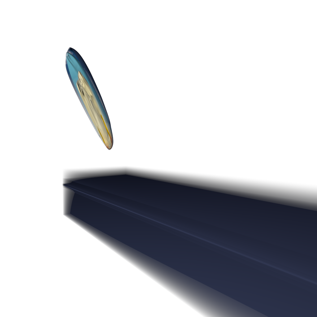
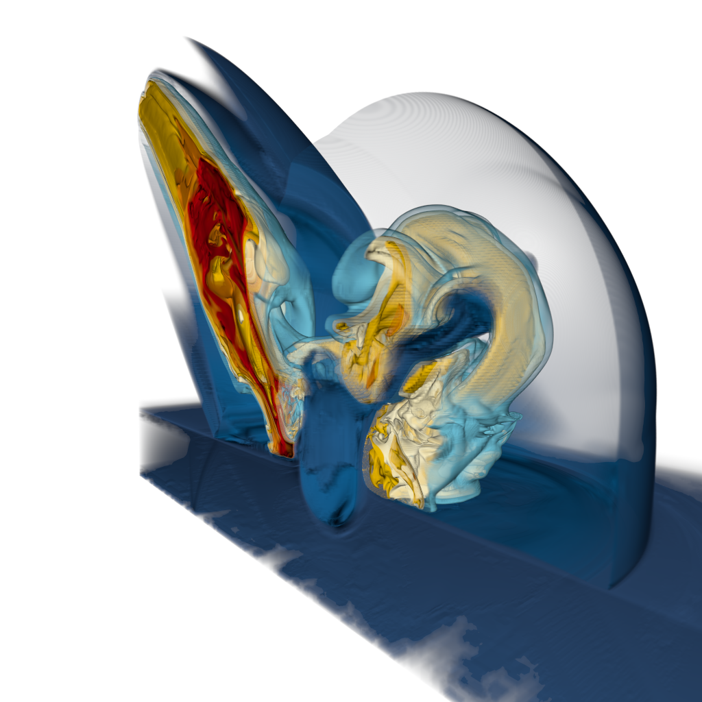
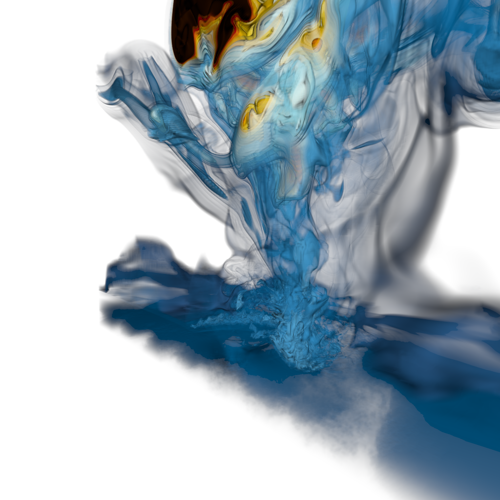
TAC Molecular Cloud	LANL Impact (t=5700)	LANL Impact (t=20060)	LANL Impact (t=46112)
102M cells, 62.5 ms	26.8M cells, 51.5 ms	158M cells, 69.6 ms	283M cells, 153.5 ms
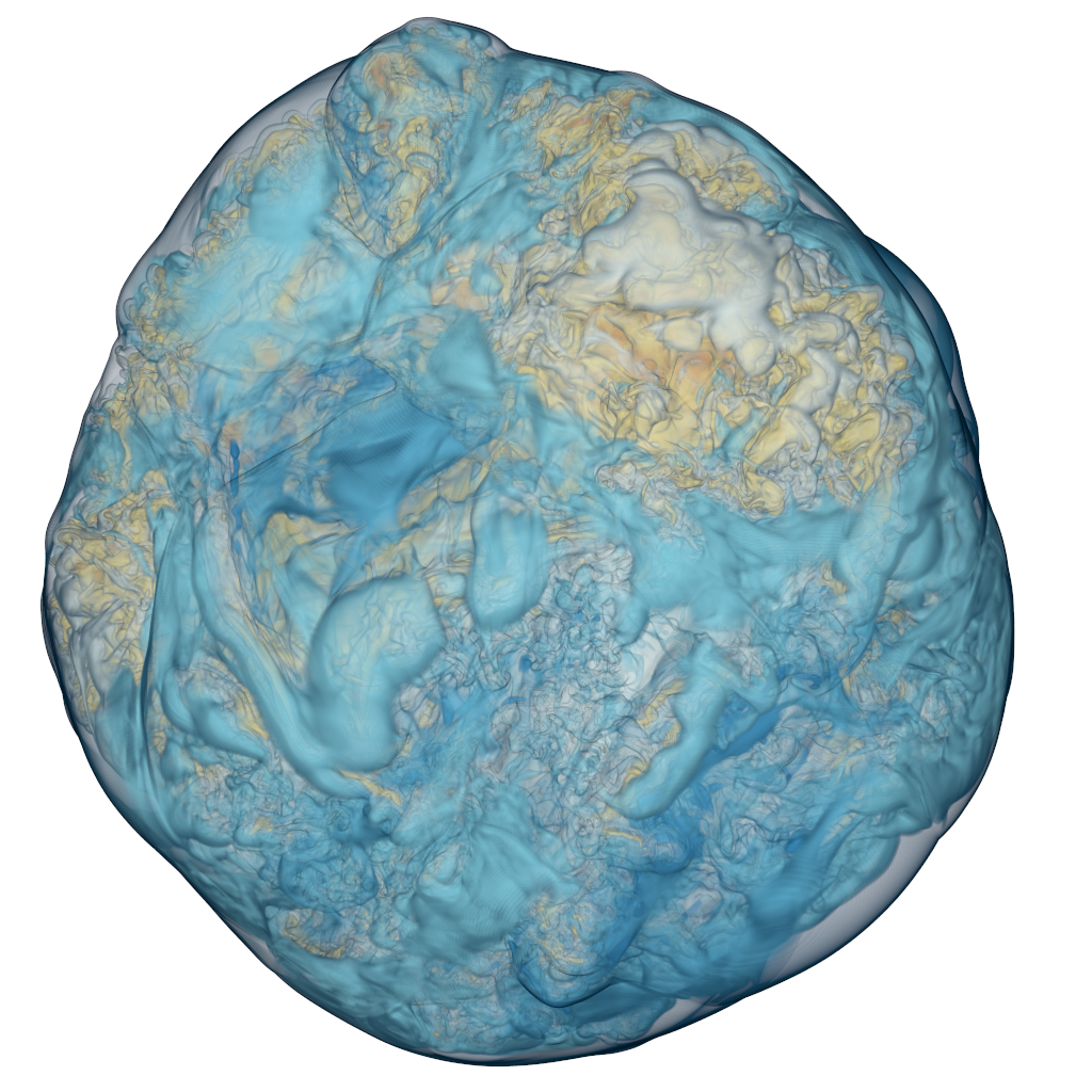
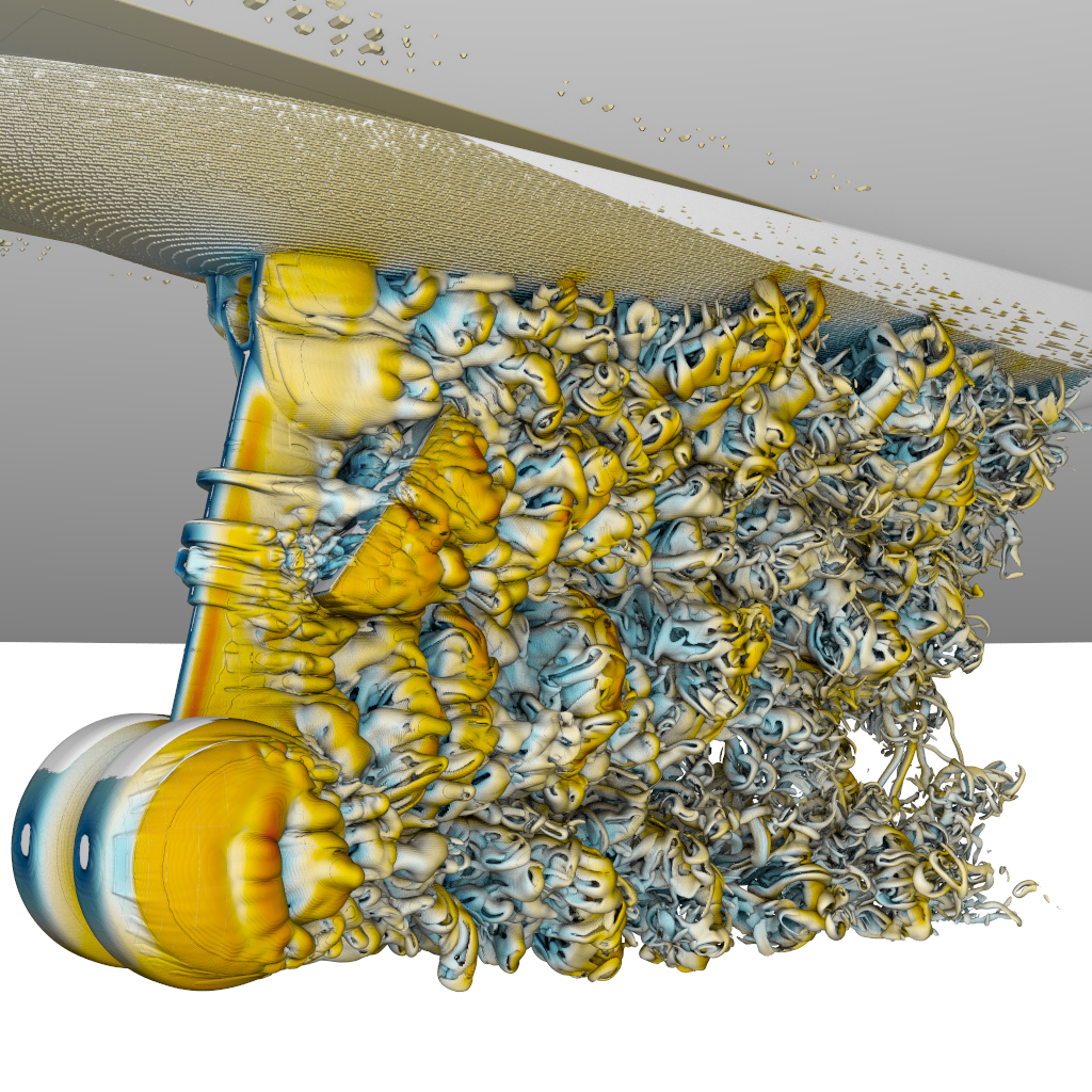
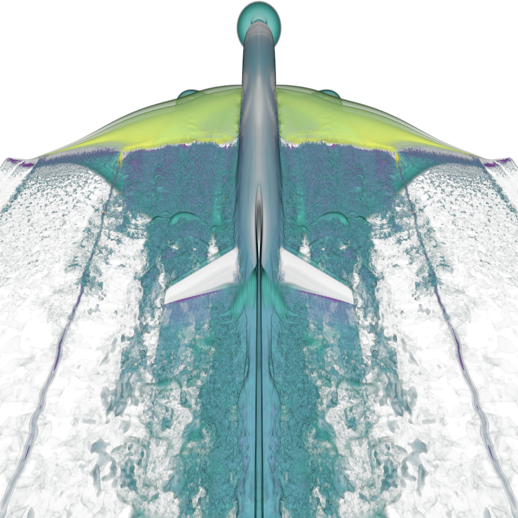
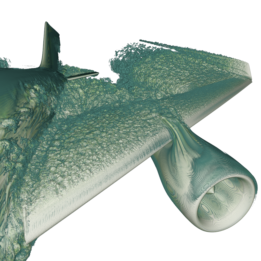
Princeton Stellar Cluster Wind	NASA Landing Gear (iso-surface)	Exajet (rear, velocity)	Exajet (wing, vorticity)
411M cells, 61.1 ms	262M cells, 1.59M tris., 71.8 ms	1.31B cells, 126M tris., 80.7 ms	1.31B cells, 126M tris., 60.1 ms

Figure 9: The data sets and benchmark visualizations used in evaluating our method. Render times are reported on a workstation with two RTX 8000 GPUs at 1024$\times$1024 pixels using the highest sampling quality settings and two AO rays per-pixel. For the LANL Impact we applied volume clipping through the middle of the data to see the plume’s interior. The Exajet is mirrored down the middle of the plane, the original data contains 656M cells and 63.2M triangles.

6 Results

To evaluate our method we performed a set of benchmarks on a range of medium to large AMR data sets (Figure 9). Our benchmarks are performed on a workstation with an Intel Xeon CPU (8 cores, 2.2 GHz), 128 GB RAM, and two NVIDIA RTX 8000 GPUs, each of which has 4608 CUDA cores, 72 RT Cores, and 48 GB of GDDR6 VRAM. We use Ubuntu 18.04, NVIDIA driver 440.44, OptiX 7.0, and CUDA 10.2.

Unless otherwise mentioned, all benchmarks are performed at the highest quality settings; i.e., using the basis method interpolant, per-sample gradient shading, surface geometry (where provided), ambient occlusion with two rays per-pixel on surface and iso-surface geometry, and an integration step size of two samples per cell. Implicit iso-surfaces are mentioned explicitly where used. The benchmarks are run using our interactive viewer, where the visualization parameters can be modified interactively by the user.

6.1 Data Sets

The structure and complexity of AMR data can vary widely among different data sets and codes. To provide a representative set of benchmarks we spent significant effort to cover a range of formats, codes, and model complexity (Figure 9).

TAC Molecular Cloud and Princeton Stellar Cluster Wind are astrophysics simulations from the Theoretical Astrophysics Group in Cologne [36] and Princeton [29], respectively; computed with the Flash simulation code [12]. Flash comes with a designated HDF5-based file format that stores the simulation grid and multiple simulation output variables in a single file, from which we extracted the AMR leaf cells.

LANL Deep Water Impact is a simulation of an Asteroid Ocean Impact computed with xRage [15] (see Patchett et al. [35]). Of particular interest for this data set is that the entire time series is available, and that the AMR structure is refined over time. Figure 9).

Landing Gear is the same data set used in previous AMR rendering research by Wald et al. [37] and Wang et al. [41]. The data set is a simulation of air flow around an airplane’s landing gear, simulated with NASA’s LAVA code [19]. To import this data set we first loaded it into OSPRay [38], and modified OSPRay’s AMR module to iterate over its AMR $k$-d tree’s leaf nodes and write out the contained cells. Of particular interest for this data set is the large ratio of the coarsest to finest cell sizes, at $4096:1$. The Landing Gear also includes 1.59M triangles in surface geometry.

Exajet is a simulation of air flow around a jet plane [5] performed using PowerFLOW [11]. The model contains 656M cells across four levels; its finest level covers a logical grid of $4.8K\times 2.4K\times 2.1K$. Of particular interest for this data set is that the interior of the airplane is not covered with cells, resulting in curved finest-level cell boundaries along the fuselage and wings. The Exajet also includes 63.15M triangles of surface geometry. As the data is cut along the symmetry down the middle of the fuselage, we create an additional instance mirrored along this axis to produce a visualization of a complete jet. After instancing, the scene contains 1.31B cells and 126M triangles.

6.2 Memory Consumption

We instrumented our code to track the sizes of the individual scalar, brick, region, and triangle data arrays, and measured final memory usage using the nvidia-smi tool (see Table 2). We note that this does not capture some additional temporary memory that OptiX uses during BVH construction. Memory consumption—and in particular, the memory used by OptiX—varies widely across the different data sets; however, even the most complex models easily fit into a Titan RTX’s or RTX 8000’s GPU memory, even with multiple fields.

Table 2: GPU memory use for the benchmarks shown in Figure 9. “Total” was measured using nvidia-smi and includes auxiliary data such as the frame buffer, accumulation buffer, and BVH memory.

	Volume Data			Surface Data	Total
Model	Scalars	Bricks	Regions
Cloud	307MB	31.8MB	1.00GB	n/a	2.06GB
Impact-5K	102MB	17.7MB	676MB	n/a	2.19GB
Impact-20K	604MB	104MB	4.82GB	n/a	12.9GB
Impact-46K	1.06GB	95.1MB	4.15GB	n/a	11.7GB
Wind	1.53GB	767KB	36.3MB	n/a	2.16GB
Gear	1.96GB	813KB	42.2MB	38.2MB	2.70GB
Exajet	2.45GB	95.0MB	2.95GB	1.52GB	13.4GB

6.3 Performance

In Ray Tracing Structured AMR Data Using ExaBricks and 9 we report average rendering times measured over 150 frames. These visualizations are representative of typical use cases for performing high-quality visualizations of AMR data; however, as with any volume renderer, the final performance is strongly tied to the transfer function chosen, as this directly affects space skipping, adaptive sample rates, and early ray termination. Therefore we also performed a scalability study where we moved the camera in a spherical orbit on the models’ bounding spheres to render 50 different viewpoints. We report rendering performance in milliseconds, along with the number of regions touched and samples taken, in Figure 10.

While for the representative visualizations (Ray Tracing Structured AMR Data Using ExaBricks and 9) we terminate rays early at an opacity threshold of 98%, we disable early ray termination for the orbit benchmark (Figure 10), to make the study less dependent on occlusion from large, homogeneous features (e.g., the ocean surface of the LANL Impact). We observe an interesting correlation between rendering performance and region size. Models that have relatively few but large regions, e.g., the Princeton Stellar Cluster Wind (170K non-empty regions) or NASA Landing Gear (283K non-empty regions), require us to take relatively more samples than models with smaller regions, e.g., the TAC Molecular Cloud (2.54M non-empty regions) or Exajet rear (15.3M non-empty regions). We also observe that performance on those models is not correlated to the number of regions touched, which indicates that the overhead of traversing the region BVH with RTX is negligible compared to the cost for the large number of samples. We also find that models with large regions with more cells have higher rendering times than those with more cells but fewer cells per region, e.g., Exajet. This suggests that models with more but smaller bricks can make better use of empty space skipping to improve performance.

Across the benchmarks our method remains interactive, even at the high quality settings chosen throughout the paper and the high resolution used in Ray Tracing Structured AMR Data Using ExaBricks. Moreover, if higher framerates or higher resolutions are desired, the user could lower the sampling rate to improve performance. We also note that, as an image-parallel approach, our method scales well as more GPUs are added to the system.

6.4 Comparison to Existing Methods

Apart from absolute performance numbers, adequately judging a method’s performance and/or quality is, generally speaking, more easily achieved by comparing it to state of the art techniques. We note that such comparisons are notoriously hard to do, as different frameworks support different hardware platforms, rendering features, or illumination models. We have identified two comparisons that stand out among the rest: First, we compare the algorithmic differences of our technique against prior approaches proposed by Kähler and Abel [16] and Wald et al. [37] (Sections 6.4.1 and 6.4.2). Second, we evaluate the performance of our complete framework against the most comparable alternative framework for rendering large-scale AMR data, OSPRay [38], in Section 6.4.3.

6.4.1 Comparison to Kähler and Abel [16]

As discussed previously, Kähler and Abel [16] propose a similar data structure to our own and construct their bricks and $k$-d tree in a nearly identical manner. They also employ ray tracing and adaptive sampling to render each brick. The core difference between our method and theirs is that they only target nearest neighbor reconstruction or vertex-centered data, avoiding the key problem that our work addresses—fast and high-quality rendering of cell-centered AMR data. Arguably, if one were to start with their framework, and incrementally add our features, such as regions for fast basis reconstruction, iso-surfaces, and analytic gradients, one would arrive at exactly the methods and algorithms described in this paper. Thus, one logical way of viewing our method is as building on the same core ideas proposed by Kähler and Abel, and improving upon it by adding a set of additional techniques such to support basis reconstruction without cell lookups, iso-surfaces, analytic gradients, and a more modern GPU implementation with RTX acceleration.

6.4.2 Comparison to Wald et al. [37]

A more recent method to compare against is that of Wald et al. [37]. Wald et al. not only proposed the basis method used in this work, but a set of reconstruction kernels that have since been further improved by Wang et al. [40, 41]. Though it should be possible to add these kernels to our framework we have not yet done so, and in particular can not yet match the reconstruction quality of Wang et al. [40].

However, we can evaluate the impact of our data structure on evaluating the basis method. To do this, we modified our brick construction algorithm to save the partitioning planes used during construction; producing effectively the same $k$-d tree used by Wald et al. [37]. We then modified our renderer to still use the regions to decide where to sample, but to ignore the list of active bricks and instead evaluate the basis method using a software cell location kernel similar to the one proposed in the original paper [37]. Both methods are run using the same settings and thus take the same samples. To keep the same rendering framework we use our fast analytic gradients for both variants, even though these were not available in the original method. The results of this experiment are given in Table 3. We find that our technique leads to a speed-up of $1.9-5.1\times$ over the original basis method, by eliminating additional cell location traversals.

Table 3: Performance of reconstruction with per-sample cell location kernels in milliseconds as originally proposed by Wald et al. [37], vs. our reconstruction from the active brick regions (Section 3.2.1).

Model	via cell loc.	from regions	speedup
	(Wald et al. [37])	(ours)
Cloud	88.5	37.8	$2.3\times$
Impact-5K	80.6	38.9	$2.1\times$
Impact-20K	258	130	$2.0\times$
Impact-46K	391	202	$1.9\times$
Wind	151	75.8	$2.0\times$
Gear	288	56.5	$5.1\times$
Exajet (rear)	218	80.6	$2.7\times$
Exajet (wing)	88.5	36.2	$2.4\times$

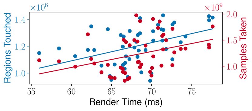
(a) TAC Molecular Cloud

(b) LANL Impact (t=5700)

(c) LANL Impact (t=20060)

(d) LANL Impact (t=46112)

(e) Princeton Stellar Cluster Wind

(f) NASA Landing Gear (iso-surface)

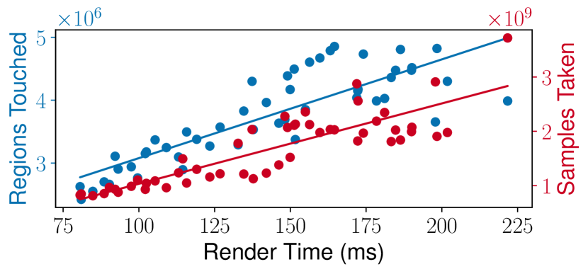
(g) Exajet (rear)

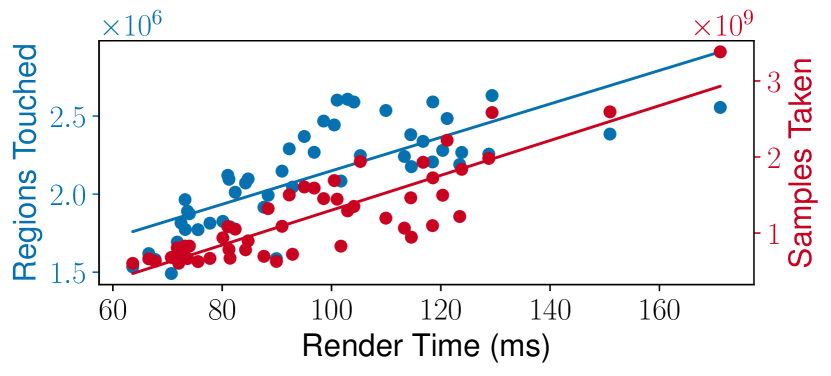
(h) Exajet (wing)

Figure 10: Rendering performance vs. the number of regions traversed and samples taken, measured over a 50 position spherical camera orbit.

6.4.3 Comparison to OSPRay

Ours	OSPRay AMR
(Default)	Similar Quality	Similar Perf.
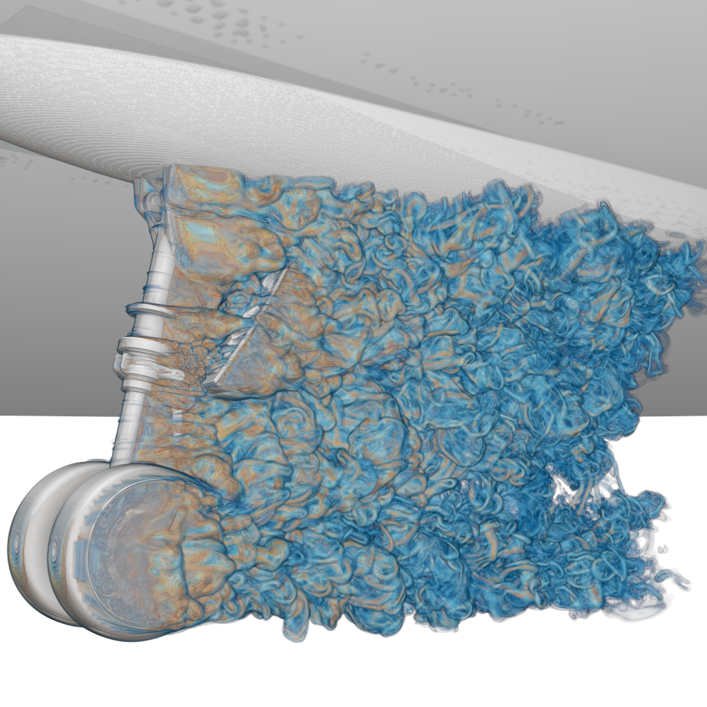
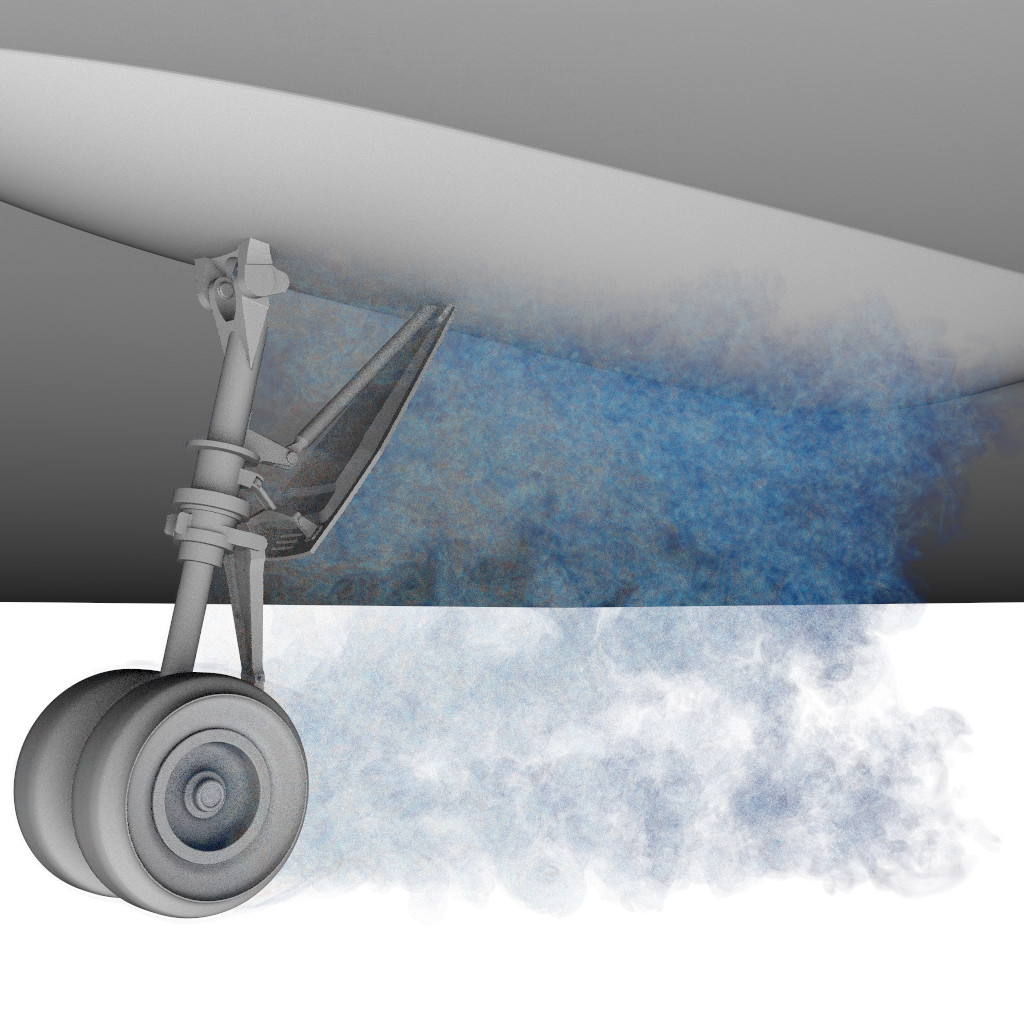
(a) 0.06 sec	(b) 12.5 sec	(c) 0.24 sec

Figure 11: Comparison to OSPRay’s native AMR rendering on the NASA Landing Gear (b) targeting similar quality or (c) performance OSPRay’s current AMR traversal does not leverage the underlying hierarchy for space skipping or adaptive sampling, leading to either poor performance at good quality (b), or poor quality for interactive performance (c).

To compare our approach to the state of the art volume rendering supported in OSPRay we took the latest version of OSPRay, imported our data sets, and tuned the transfer function and sampling rate to achieve either similar performance or roughly similar quality. We note that comparisons between two different frameworks are always apples-to-oranges, and that the output images will never fully match. For example, our method performs adaptive sampling, while OSPRay ray marches at a fixed step size; similarly, our method always performs gradient shading and lighting, while OSPRay does not (compare, e.g., Figure 12a and b). For these experiments, we ran OSPRay on a high-end workstation equipped with a Xeon W-3275M 28-core “Cascade Lake” CPU and 256 GB of RAM.

OSPRay provides native support for rendering Block-Structured AMR, such as the NASA Landing Gear, which we perform a direct comparison with in Figure 11. Though any such comparison has to be taken with a grain of salt, the general observation is that our system achieves either significantly higher quality at similar performance, or higher performance at similar quality.

Although OSPRay offers native support for Block-Structured AMR, it does not support Tree-Based AMR variants, a limitation shared by standard tools such as ParaView and VisIt. For AMR data that does not fit OSPRay’s requirements (e.g., Exajet and LANL Impact), an alternative approach to rendering such data is to first convert it to an unstructured mesh by computing its dual mesh, then render the resulting mesh using OSPRay’s unstructured mesh renderer.

While flattening the data allows scientists to visualize it using standard tools, it is far from ideal. The resulting unstructured mesh occupies significantly more memory than the original data and is more challenging to render due to the now unstructured layout (Figure 12). Consequently the observation of “better performance at similar quality or better quality at similar performance” is more pronounced in this comparison (Figure 12).

Ours	OSPRay Unstructured
(Default)	Similar Quality	Similar Perf.
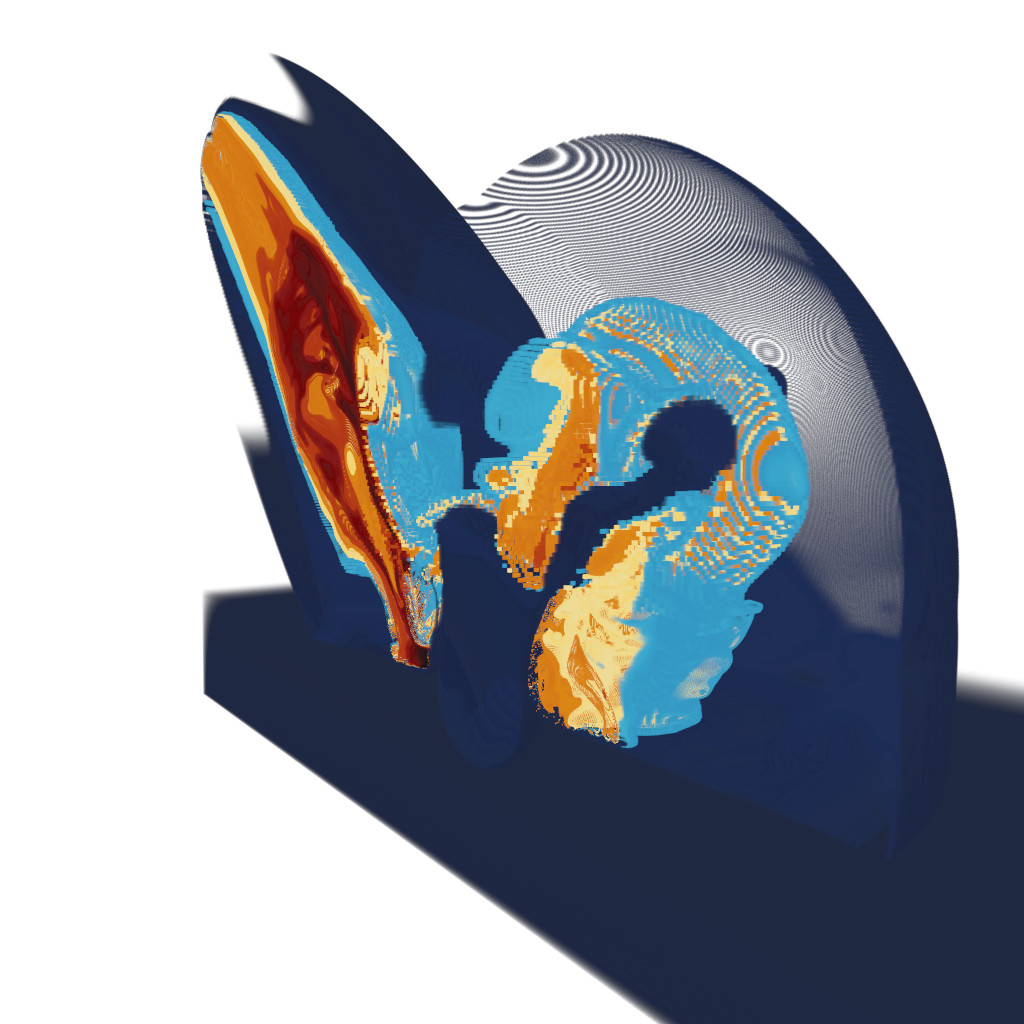
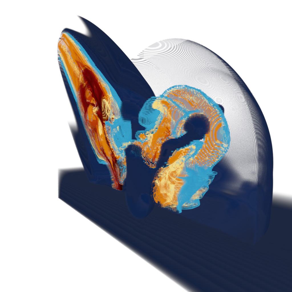
(a) 69.6 ms	(b) 435 ms	(c) 133 ms
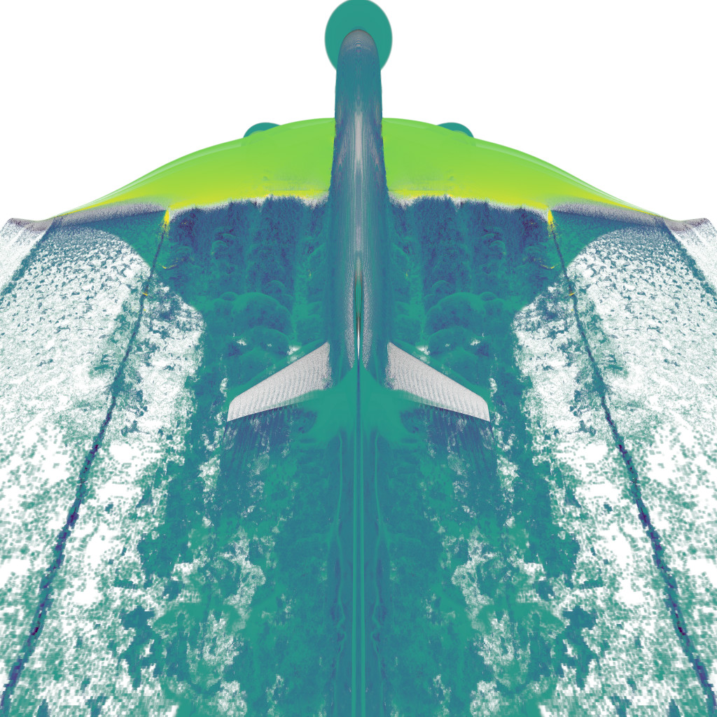
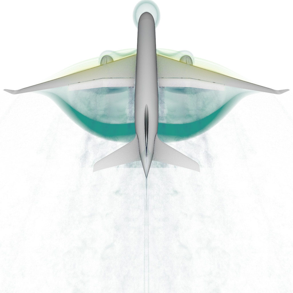
(d) 80.1 ms	(e) 3.33 sec	(f) 185 ms

Figure 12: Quality and performance comparisons against rendering the AMR data as an unstructured mesh using OSPRay. The unstructured mesh requires significantly more memory (b,c: 40 GB, e,f: 160 GB), and trading performance for image quality (b,e) or vice-versa (c, f).

7 Limitations

Our presented ExaBricks data structure is suitable for high-quality interactive rendering of the large scale AMR data sets used in simulations today. However, our approach is not without limitations. We currently only support the basis method for sample reconstruction, and while methods such as octant [41] or GTI [40] should be possible to add, doing so would require reexamining what the support of a cell (and thus, brick) looks like.

Another potential limitation of our method is that its performance and memory consumption depend on the number and distribution of bricks a data set is partitioned into. For example, on the Exajet the curved empty regions around the plane geometry result in a large number of single-cell bricks. While our space skipping and adaptive sampling strategies reduce the impact of such bricks, they do not come without cost. A potential option to address this would be to allow for partially filled bricks. Similarly, the number and distribution of the active brick regions can become non-trivial, challenging the BVH construction or traversal. To this end, future work on improving the builder to produce less, and possibly less exact, regions could be valuable. Finally, we do not take advantage of hardware texture interpolation in our method, as the large number of bricks may require a substantial number of textures or a large atlas. However, this could further improve rendering performance by accelerating sample computation.

Arguably more important than the output brick or region distribution, is that neither is computed in real time in our current implementation. The bricks are constructed in an offline pre-process and can take several minutes, while the regions are built at load time and can take tens of seconds. Both steps can likely be accelerated significantly, and would improve the experience for future end users.

From a practical standpoint, the biggest limitation of our framework is that it is not yet available within a standard visualization package. Although we plan to make our source code available, making these capabilities available to end users would require an integration into ParaView [2] or VisIt [6]. Such an integration would address a clear need in the AMR community and could be done through an integration into OSPRay [38] or IndeX [30], which are already used by these tools.

8 Conclusion

In this paper, we have proposed a novel approach for high-quality and efficient rendering of AMR data, through a combination of three inter-operating data structures. We have demonstrated our method’s capabilities on a set of non-trivial models, and have shown that it is capable of achieving interactive performance on a single workstation for large models and demanding high-quality rendering settings, and is competitive with the state of the art. A key advantage of our method is its generality, both in how easily it can be adapted to support different AMR formats, and in how it lends itself to implementation in other rendering frameworks. Although the presented implementation leverages GPU hardware ray tracing, there is no reason the same approach could not be implemented in a CPU framework such as OSPRay.

The key to our approach is our ExaBricks data structure—and in particular the Active Brick Regions—which provide the “glue” that allows for seamlessly combining several known techniques (bricking AMR data, basis reconstruction, space skipping, adaptive sampling, RTX volume traversal) into a single algorithmic framework in which they operate on the same set of active brick regions and work to each other’s advantage. Our approach for combining these techniques forms a compelling blueprint for high-quality AMR rendering, and serves as an example which may be adopted in standard visualization packages.

- [1] M. Aftosmis, M. Berger, and G. Adomavicius. A Parallel Multilevel Method for Adaptively Refined Cartesian Grids with Embedded Boundaries. Technical Report AIAA-00-0808, American Institute of Aeronautics and Astronautics, 2000. 38th Aerospace Sciences Meeting and Exhibit.
- [2] U. Ayachit. The ParaView Guide: A Parallel Visualization Application. Kitware, Inc., 2015.
- [3] M. J. Berger and J. Oliger. Adaptive Mesh Refinement for Hyperbolic Partial Differential Equations. Journal of Computational Physics, 1984.
- [4] J. Beyer, M. Hadwiger, and H. Pfister. State-of-the-Art in GPU-Based Large-Scale Volume Visualization. Computer Graphics Forum, 2015.
- [5] D. Casalino and A. Hazir. Lattice Boltzmann based Aeroacoustic Simulation of Turbofan Noise Installation Effects. In 23rd International Congress on Sound and Vibration, 2014.
- [6] H. Childs. VisIt: An End-User Tool for Visualizing and Analyzing Very Large Data. 2012.
- [7] K. Clough, P. Figueras, H. Finkel, M. Kunesch, E. A. Lim, and S. Tunyasuvunakool. Numerical Relativity with Adaptive Mesh Refinement. Classical and Quantum Gravity, 2015.
- [8] P. Colella, D. Graves, T. Ligocki, D. Martin, D. Modiano, D. Serafini, and B. Van Straalen. Chombo Software Package for AMR Applications Design Document, 2000.
- [9] R. A. Drebin, L. Carpenter, and P. Hanrahan. Volume Rendering. ACM SIGGRAPH Computer Graphics (Proceedings of the 15th Annual Conference on Computer Graphics and Interactive Techniques - SIGGRAPH ’88), 1988.
- [10] K. Engel, M. Hadwiger, J. Kniss, C. Rezk-Salama, and D. Weiskopf. Real-Time Volume Graphics. 2006.
- [11] PowerFLOW User’s Guide 3.0, 1998.
- [12] B. Fryxell, K. Olson, P. Ricker, F. X. Timmes, M. Zingale, D. Q. Lamb, P. MacNeice, R. Rosner, J. W. Truran, and H. Tufo. FLASH: An Adaptive Mesh Hydrodynamics Code for Modeling Astrophysical Thermonuclear Flashes. The Astrophysical Journal Supplement Series, 2000.
- [13] D. Ganter and M. Manzke. An Analysis of Region Clustered BVH Volume Rendering on GPU. In Proceedings of High Performance Graphics (HPG), 2019.
- [14] J. D. d. S. Germain, J. McCorquodale, S. G. Parker, and C. R. Johnson. Uintah: A Massively Parallel Problem Solving Environment. In Proceedings the Ninth International Symposium on High-Performance Distributed Computing, 2000.
- [15] M. Gittings, R. Weaver, M. Clover, T. Betlach, N. Byrne, R. Coker, E. Dendy, R. Hueckstaedt, K. New, W. R.Oakes, D. Ranta, and R. Stefan. The RAGE Radiation-Hydrodynamic Code. Computational Science & Discovery, 2008.
- [16] R. Kähler and T. Abel. Single-Pass GPU-Raycasting for Structured Adaptive Mesh Refinement Data. arXiv:1212.3333 [astro-ph], 2013.
- [17] R. Kähler, J. Wise, T. Abel, and H.-C. Hege. GPU-Assisted Raycasting for Cosmological Adaptive Mesh Refinement Simulations. In Volume Graphics, 2006.
- [18] A. Keller and W. Heidrich. Interleaved Sampling. In Rendering Techniques 2001 (Proceedings of the Eurographics Workshop on Rendering). 2001.
- [19] C. C. Kiris, M. F. Barad, J. A. Housman, E. Sozer, C. Brehm, and S. Moini-Yekta. The LAVA Computational Fluid Dynamics Solver. 52nd Aerospace Sciences Meeting, AIAA SciTech Forum, 2014.
- [20] M. Labadens, D. Chapon, D. Pomaréde, and R. Teyssier. Visualization of Octree Adaptive Mesh Refinement (AMR) in Astrophysical Simulations. In Astronomical Data Analysis Software and Systems XXI, ASP Conference Series. 2011.
- [21] N. Leaf, V. Vishwanath, J. Insley, M. Hereld, M. E. Papka, and K.-L. Ma. Efficient parallel volume rendering of large-scale adaptive mesh refinement data. In 2013 IEEE Symposium on Large-Scale Data Analysis and Visualization (LDAV), 2013.
- [22] M. Levoy. Display of Surfaces from Volume Data. IEEE Computer Graphics and Applications, 1988.
- [23] P. Ljung. Adaptive Sampling in Single Pass, GPU-based Raycasting of Multiresolution Volumes. In Volume Graphics 2006: Eurographics, 2006.
- [24] P. Ljung, C. Lundström, and A. Ynnerman. Multiresolution Interblock Interpolation in Direct Volume Rendering. In EUROVIS - Eurographics /IEEE VGTC Symposium on Visualization, 2006.
- [25] K.-L. Ma. Parallel Rendering of 3D AMR Data on the SGI/Cray T3E. In Proceedings of the The 7th Symposium on the Frontiers of Massively Parallel Computation. 1999.
- [26] N. L. Max. Sorting for Polyhedron Compositing. In Focus on Scientific Visualization, 1991.
- [27] P. Moran and D. Ellsworth. Visualization of AMR Data with Multi-Level Dual-Mesh Interpolation. IEEE Transactions on Visualization and Comput Graphics (TVCG), 2011.
- [28] N. Morrical, W. Usher, I. Wald, and V. Pascucci. Efficient Space Skipping and Adaptive Sampling of Unstructured Volumes Using Hardware Accelerated Ray Tracing. In Proceedings of IEEE Visualization (Short Papers Track), 2019.
- [29] J. P. Naiman, M. Soares-Furtado, and E. Ramirez-Ruiz. Modelling Gas Evacuation Mechanisms in Present-Day Globular Clusters: Stellar Winds from Evolved Stars and Pulsar Heating. Monthly Notices of the Royal Astronomical Society, 2019.
- [30] NVIDIA Index. https://developer.nvidia.com/nvidia-index.
- [31] B. W. O’shea, G. Bryan, J. Bordner, M. L. Norman, T. Abel, R. Harkness, and A. Kritsuk. Introducing Enzo, an AMR Cosmology Application. In Adaptive mesh refinement-theory and applications, Lecture Notes in Computational Science and Engineering. Springer, 2005.
- [32] S. Park, C. L. Bajaj, and V. Siddavanahalli. Case Study: Interactive Rendering of Adaptive Mesh Refinement Data. In Proceedings of IEEE Visualization, 2002.
- [33] S. Parker, M. Parker, Y. Livnat, P.-P. Sloan, C. Hansen, and P. Shirley. Interactive Ray Tracing for Volume Visualization. IEEE Transactions on Visualization & Computer Graphics, 1999.
- [34] S. G. Parker, J. Bigler, A. Dietrich, H. Friedrich, J. Hoberock, D. Luebke, D. McAllister, M. McGuire, K. Morley, and A. Robison. OptiX: A General Purpose Ray Tracing Engine. ACM Transactions on Graphics (Proceedings of ACM SIGGRAPH), 2010.
- [35] J. M. Patchett, F. J. Samsel, K. C. Tsai, G. R. Gisler, D. H. Rogers, G. D. Abram, and T. L. Turton. Visualization and Analysis of Threats from Asteroid Ocean Impacts. Technical report, Los Alamos National Laboratory, 2016.
- [36] D. Seifried, S. Walch, P. Girichidis, T. Naab, R. Wünsch, R. S. Klessen, S. C. O. Glover, T. Peters, and P. Clark. SILCC-Zoom: the dynamic and chemical evolution of molecular clouds. Monthly Notices of the Royal Astronomical Society, 472(4):4797–4818, Dec 2017. doi: 10 . 1093/mnras/stx2343
- [37] I. Wald, C. Brownlee, W. Usher, and A. Knoll. CPU Volume Rendering of Adaptive Mesh Refinement Data. In SIGGRAPH Asia 2017 Symposium on Visualization, 2017. doi: 10 . 1145/3139295 . 3139305
- [38] I. Wald, G. P. Johnson, J. Amstutz, C. Brownlee, A. Knoll, J. Jeffers, J. Günther, and P. Navrátil. OSPRay – A CPU Ray Tracing Framework for Scientific Visualization. IEEE Transactions on Visualization and Computer Graphics, 2017.
- [39] I. Wald, W. Usher, N. Morrical, L. Lediaev, and V. Pascucci. RTX Beyond Ray Tracing: Exploring the Use of Hardware Ray Tracing Cores for Tet-Mesh Point Location. In Proceedings of High Performance Graphics, 2019.
- [40] F. Wang, N. Marshak, W. Usher, C. Burstedde, A. Knoll, T. Heister, and C. R. Johson. CPU Ray Tracing of Tree-Based Adaptive Mesh Refinement Data. Computer Graphics Forum, 2020.
- [41] F. Wang, I. Wald, Q. Wu, W. Usher, and C. R. Johnson. CPU Isosurface Ray Tracing of Adaptive Mesh Refinement Data. IEEE Transactions on Visualization and Computer Graphics, 2019.
- [42] G. H. Weber, H. Childs, and J. S. Meredith. Efficient Parallel Extraction of Crack-Free Isosurfaces from Adaptive Mesh Refinement (AMR) Data. In 2012 IEEE Symposium on Large Data Analysis and Visualization, 2012.
- [43] G. H. Weber, O. Kreylos, T. J. Ligocki, J. M. Shalf, H. Hagen, B. Hamann, and K. I. Joy. Extraction of Crack-Free Isosurfaces from Adaptive Mesh Refinement Data. In Hierarchical and Geometrical Methods in Scientific Visualization. 2003.