Prediction of aerothermal characteristics of a generic hypersonic inlet flow

Abstract

Accurate prediction of aerothermal surface loading is of paramount importance for the design of high speed flight vehicles. In this work, we consider the numerical solution of hypersonic flow over a double-finned geometry, representative of the inlet of an air-breathing flight vehicle, characterized by three-dimensional intersecting shock-wave/turbulent boundary-layer interaction at Mach 8.3. High Reynolds numbers ($Re_{L}\approx 11.6\times 10^{6}$ based on free-stream conditions) and the presence of cold walls ($T_{w}/T_{\circ}\approx 0.26$) leading to large near-wall temperature gradients necessitate the use of wall-modeled large-eddy simulation (WMLES) in order to make calculations computationally tractable. The comparison of the WMLES results with experimental measurements shows good agreement in the time-averaged surface heat flux and wall pressure distributions, and the WMLES predictions show reduced errors with respect to the experimental measurements than prior RANS calculations. The favorable comparisons are obtained using a standard LES wall model based on equilibrium boundary layer approximations despite the presence of numerous non-equilibrium conditions including three dimensionality in the mean, shock-boundary layer interactions, and flow separation. We demonstrate that the use of semi-local eddy viscosity scaling (in lieu of the commonly used van Driest scaling) in the LES wall model is necessary to accurately predict the surface pressure loading and heat fluxes.

1 Introduction

Hypersonic wall-bounded flows for realistic flight vehicles can be characterized by high Reynolds numbers and cold surface temperatures compared to the free-stream stagnation temperature. The prohibitive computational cost associated with high Reynolds numbers are well known choi2012grid , while the cold wall conditions exacerbate near-wall resolution requirements associated with the large temperature gradients in the vicinity of peak viscous dissipation. As a result, direct numerical simulations of these flows have been largely limited to simple geometries and low Reynolds numbers such as high-speed compressible boundary layer flows duan2011directMach , hypersonic boundary-layer transitional flow for a flared cone hader2019direct , turbulent boundary layer along a compression ramp adams2000direct , and transitional shock/boundary-layer interaction sandham2014transitional Fu2020Direct .

When more realistic geometries and conditions are considered, the RANS approach is commonly used in industrial settings due to reduced computational costs compared to DNS strategies. However, RANS based approaches have been demonstrated to have limited accuracy in hypersonic flow regimes; significant errors in peak aerodynamic heating ($\approx 25\%$) currao2019hypersonic are observed and macroscopic flow characteristics are misrepresented, in particular when laminar/turbulent transition or boundary layer separation are present georgiadis2014status fu2013rans . Cold wall conditions in hypersonic flow regimes also challenge traditional RANS models (e.g., Spalart-Allmaras, $k-\omega$) to predict near-wall turbulent fluctuations or transverse heat fluxes huang2019assessment even in zero-pressure gradient boundary layers. Algebraic RANS closures, such as the Baldwin-Lomax model baldwin1978thin , have been shown to offer reasonable predictions in high Mach number boundary layer flows rumsey2010compressibility . However, application of these models to the double-finned inlet flow presently considered show substantial errors in the surface heat fluxes and in the extent of flow separation gaitonde1993calculations .

Large-eddy simulations have been shown to offer superior accuracy in the prediction of many of these flow regimes. However, it is well known that near-wall resolution requirements for LES are prohibitive in high Reynolds number conditions. Alternatively, the WMLES approach, where flow structures that scale with the boundary layer thickness are resolved while effects of unresolved near-wall eddies (at viscous length scales, $l_{\nu}=\nu/u_{\tau}$) are modeled, has been shown to be computationally tractable for high Reynolds number flows and predictive in several complex flows bose2018wall . In the context of high-speed flows, WMLES has been successfully applied to the prediction of shock-induced separation kawai2013dynamic souverein2010effect , oblique shock wave interaction with lateral confinement and boundary layer separation bermejo2014confinement helmer2012three , transitional flows mettu2018wall , and aerodynamic heating yang2017aerodynamic Fu2020Direct . However, most of the high speed applications of WMLES have been conducted in relatively simple geometries or in the absence of technologically relevant cold wall conditions.

To this end, the present work considers a canonical model of a realistic inlet of an air-breathing hypersonic vehicle kussoy1992intersecting . The configuration consists of two sharp fins mounted on a flat plate. An incident hypersonic turbulent boundary layer approaches the two vertical fins generating a crossing shock pattern resulting in high local aerothermal loading and flow separation. The objective of this investigation is to assess the predictive capability of of wall modeled LES in this complex geometry and flow regime with emphasis on the prediction of surface heat fluxes, mechanical loading, and separation that arises from the impinging shock structure. WMLES results are strictly grid dependent since the grid size $\Delta$ appears in the governing equations through the subgrid and wall model formulae deployed. The models used in the present WMLES do converge to DNS solutions in the limit of very fine resolutions. However, the main question that we seek to answer is whether quantities of interest can be predicted with acceptable accuracy at affordable cost. Specifically, the trade-off between accuracy and resolution requirements is not well understood in complex flows, particularly those with mild separations. This investigation attempts to characterize the threshold resolution for sufficiently accurate simulations in this double fin configuration.

The remainder of this paper is organized as follows. In Section 2, the governing equations, the wall model and the numerical method are briefly reviewed. In Section 3, the flow conditions and corresponding computational setup are described. Section 4 analyzes the WMLES results, including detailed spatial structures of the mean flow, and assesses their accuracy with respect to existing experimental measurements and prior RANS simulations. It is additionally demonstrated that the cold wall conditions in this configuration necessitate augmentation of wall model eddy viscosity to be scaled on semi-local conditions rather than solely on wall quantities typically used in prior WMLES calculations. Concluding remarks and discussions are provided in Section 5. In the Appendix, convergence of the results with longer statistical averaging time (statistical sample size) and finer grid resolution is discussed.

2 LES methodology

2.1 LES governing conservation equations

The Favre-averaged compressible Navier-Stokes equations in the conservative form are

$$\frac{{\partial\overline{\rho}}}{{\partial t}}+\frac{{\partial\overline{\rho}\widetilde{{u}_{j}}}}{{\partial{x_{j}}}} = 0,$$ (1)

$$\frac{{\partial\overline{\rho}\widetilde{{u_{i}}}}}{{\partial t}}+\frac{{\partial\overline{\rho}\widetilde{{u_{i}}}\widetilde{{u_{j}}}}}{{\partial{x_{j}}}}+\frac{{\partial\overline{P}}}{{\partial{x_{i}}}} = \frac{{\partial\widetilde{{\sigma_{ij}}}}}{{\partial{x_{j}}}}-\frac{{\partial{\tau_{ij}^{sgs}}}}{{\partial{x_{j}}}},$$ (2)

$$\frac{{\partial\overline{E}}}{{\partial t}}+\frac{{\partial[(\overline{E}+\overline{P}){\widetilde{{u_{j}}}]}}}{{\partial{x_{j}}}} = \frac{{\partial}}{{\partial{x_{j}}}}(k\frac{{\partial\overline{T}}}{{\partial{x_{j}}}})+\frac{{\partial(\widetilde{u_{i}}{\widetilde{{\sigma_{ij}}})}}}{{\partial{x_{j}}}}-\frac{{\partial{Q_{j}^{sgs}}}}{{\partial{x_{j}}}}-\frac{{\partial\left({\widetilde{u_{i}}}{\tau_{ij}^{sgs}}\right)}}{{\partial{x_{j}}}},$$ (3)

where $\rho$, $P$, and $T$ denote the fluid density, pressure, and temperature, respectively. $u_{i}$ denotes the velocity component in the $x_{i}$ coordinate direction. $\overline{E}=\bar{\rho}\tilde{e}+\overline{\rho}\widetilde{{u_{k}}}\widetilde{{u_{k}}}/2$ denotes the total energy, $\widetilde{{\sigma_{ij}}}=\mu(\tilde{T})(\widetilde{S}_{ij}-1/3\widetilde{S}_{kk}\delta_{ij})$ is the resolved deviatoric stress tensor, and $\widetilde{S}_{ij}=1/2({\partial{\widetilde{u}_{i}}}/{\partial{x_{j}}}+{\partial\widetilde{u_{j}}}/{\partial{x_{i}}})$ is the resolved strain rate tensor. The subgrid stress ${\tau_{ij}^{sgs}}$ and heat flux ${Q_{j}^{sgs}}$ arising from the effect of unresolved eddies are defined as

$${\tau_{ij}^{sgs}}=\overline{\rho}(\widetilde{u_{i}u_{j}}-\widetilde{u_{i}}\widetilde{u_{j}}),\text{ }{Q_{j}^{sgs}}=\overline{\rho}(\widetilde{eu_{j}}-\widetilde{e}\widetilde{u_{j}}),$$ (4)

The subgrid stresses and heat fluxes are closed with the Vreman eddy viscosity model vreman2004eddy supplemented with a constant turbulent Prandtl number ($Pr_{t}=0.9$). The equation of state for the fluid is a calorically perfect gas, $\bar{P}=\bar{\rho}R\tilde{T}$, where $R$ denotes the specific gas constant. The relation between the dynamic viscosity and the temperature is characterized by the Sutherland’s law with a model constant $S/T_{r}=1.38,T_{r}=80$ K, and the Prandtl number is $0.72$. The calorically perfect gas assumption is adopted based on the low free-stream temperature for the configuration under consideration, $T_{\infty}=80$ K. Hereafter, the operator symbols $\bar{\cdot}$ and $\tilde{\cdot}$ denote the Reynolds and Favre averages, respectively. $f^{{}^{\prime}}=f-\bar{f}$ denotes the fluctuation defined based on the Reynolds average, and $f^{{}^{\prime\prime}}=f-\overline{\rho f}/\bar{\rho}$ denotes the fluctuation defined based on the Favre average.

2.2 LES wall model based on equilibrium boundary layer approximations

As the near-wall eddies with length scales characterized by viscous length scales are not resolved in the present formulation, their aggregate effect on the wall stress and heat flux must be modeled. (For a detailed description and review of the wall models for LES, see bose2018wall larsson2016large wangmoin2002 ). The present LES wall model assumes that the pressure gradient and convection effects can be neglected for unresolved eddies between the wall and the local LES resolution (of grid size, $\Delta$), and that these eddies reach a statistically stationary state over the duration of the simulation time step ($\Delta t$). With these approximations, the simplified momentum and total energy equations can be written as kawai2012wall

$$\frac{d}{{dy}}\left[{(\bar{\mu}+{\bar{\mu}_{t,wm}})\frac{{d{\bar{u}_{\parallel}}}}{{dy}}}\right]=0,$$ (5)

$$\frac{d}{{dy}}\left[{(\bar{\mu}+{\bar{\mu}_{t,wm}}){\bar{u}_{\parallel}}\frac{{d{\bar{u}_{\parallel}}}}{{dy}}+{c_{p}}\left(\frac{\bar{\mu}}{{Pr}}+\frac{{{\bar{\mu}_{t,wm}}}}{{{{Pr}_{t,wm}}}}\right)\frac{{d\bar{T}}}{{dy}}}\right]=0,$$ (6)

where $y$ and $\bar{u}_{\parallel}$ denote the wall-normal coordinate and the velocity component parallel to the wall, respectively. $c_{p}$, and $Pr$ denote the specific heat capacity at constant pressure, and the molecular Prandtl number, respectively. Turbulent stresses and heat fluxes are modeled with an eddy viscosity, $\bar{\mu}_{t,wm}$, given by the mixing length model,

$${\bar{\mu}_{t,wm}}=\kappa\bar{\rho}y\sqrt{\frac{{{\bar{\tau}_{w}}}}{\bar{\rho}}}D,$$ (7)

where $\kappa=0.41$ is the von Kármán constant, the damping function $D$ is defined as

$$D=\left[1-\exp\left(-\frac{{y_{vD}^{+}}}{A^{+}}\right)\right]^{2},$$ (8)

where $A^{+}=17$, and ${y_{vD}^{+}}={y}/({{{\bar{\nu}_{w}}/{\bar{u}_{\tau}}}})$, $\bar{\nu}_{w}$ and $\bar{u}_{\tau}$ denote the kinematic viscosity and friction velocity at the wall. However, it is shown in iyer2019analysis yang2018semi that the van Driest transformation performs poorly in collapsing the compressible velocity profile onto the incompressible counterpart for wall-bounded flows with cold wall condition. Due to this, we additionally consider in this work a semi-local scaling huang1995compressible ; patel2015semi ; iyer2019analysis ; muto2019equilibrium

$$y_{SL}^{+}=\frac{{\bar{\rho}(y){\sqrt{\left({{\bar{\tau}_{w}}/\bar{\rho}(y)}\right)}}y}}{\bar{\mu}(y)},$$ (9)

where the dynamic viscosity is computed based on the local conditions at a off-wall distance, $y$, and $y_{SL}^{+}$ is used in place of $y_{vD}^{+}$ in Eq. (8). While the semi-local scaling has been used to treat variable property effects close to the wall and explore the collapse of canonical equilibrium boundary layers, its a posteriori impact for wall modeled LES in a non-equilibrium, hypersonic flow is presently not well understood. This semi-local scaling is shown below to have significant effects on the prediction of the non-equilibrium flow, especially in the non-equilibrium boundary layer flow between the fins.

The boundary conditions for Eqns. (5) and (6) for the velocity and temperature are no-slip, isothermal conditions at the wall ($\bar{u}_{||}(y=0)=0,\bar{T}(y=0)=T_{w}$) and the interior LES conditions ($\bar{u}_{||}(h_{wm})=\tilde{u}_{\rm{LES}},\bar{T}(h_{wm})=\tilde{T}_{\rm{LES}}$) at a distance, $h_{wm}$, from the wall. In this work, the matching location is chosen as the first off-wall cell center in the local wall-normal direction. It is important to note that while the wall model does not explicitly contain the non-equilbirium pressure gradient or convection effects, the influence of these phenomena are implicitly present in the time dependent far field boundary condition that the interior LES provides at the interface of the wall model region.

2.3 Numerical methods

The compressible, finite-volume code $\rm charLES$ bres2018large , is used to conduct the numerical simulations herein. The numerical method consists of a low-dissipation, approximate entropy-preserving scheme and utilizes artificial bulk viscosity to capture solution discontinuities mani2009suitability . The LES governing equations are temporally integrated by the explicit third-order strong-stability-preserving (SSP) Runge-Kutta method gottlieb2001 . The spatial and temporal schemes converge to second- and third-order with respect to the nominal mesh spacing and time step, respectively. Computational meshes based on arbitrary polyhedra are constructed from the computation of Voronoi diagrams aurenhammer1991voronoi . Details of the numerical method and solver validation campaigns can be found in Fu2020Direct , lozano2020 , lakebrink2019 , bres2019modelling , bres2018large , and lehmkuhl2018 .

3 Double-finned problem definition and computational setup

The present geometry and computational setup follow those described in the experiment of a $15^{\circ}$ double-finned configuration kussoy1992intersecting . The geometry is composed of two sharp fins with wedge angle $\alpha=15^{\circ}$ fastened to a flat plate, as shown in Fig. 1. Specifically, each fin is $20$ cm high and $40.6$ cm long, and the flat plate is $220$ cm long and $10$ cm high. The double fins are placed $165$ cm downstream of the leading edge of the flat plate such that there is sufficient length for a turbulent boundary layer to develop. The free-stream flow measured $3$ cm ahead of the double fins (i.e. at $x_{\circ}=162$ cm) has a Mach number $Ma_{\infty}=8.23$ and Reynolds number $Re_{\delta_{\circ}}=1.7\times 10^{5}$ based on the local boundary layer thickness ($\delta_{\circ}=3.25$ cm). The wall is isothermal at $T_{w}=300$ K which is substantially colder than the stagnation temperature $T_{\circ}=1177$ K. In the following discussion, velocity, temperature, density and length are normalized by the sound speed $c_{r}=179$ m/s, the reference temperature $T_{r}=80$ K, the reference density $\rho_{r}=0.0186$ $\rm{kg/m^{3}}$ and the reference length $L_{r}=1$ cm.

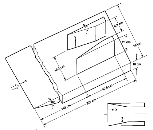
Figure 1: The geometry parameters and the computational coordinate system. The wedge angle for the double fins is $\alpha=15^{\circ}$. The arrow indicates that the fluid flows from the leading edge of the flat plate towards the double fins. The leading edges of both the flat plate and the double fins are sharp and the model is symmetric with respect to the plane $z=0$ cm. The free-stream condition is defined $3$ cm ahead of the double fins at $x_{\circ}=162$ cm. This figure is adapted from Fig. 1 of kussoy1992intersecting .

The computational geometry is given in Fig. 2(a). The computational domain is sufficiently large to minimize artificial reflections from the far-field outflow boundaries.

The inlet flow condition is imposed by combining a uniform flow with turbulence fluctuations generated by a synthetic turbulence generation method wu2017inflow . The entry length of the domain is not of sufficient extent to replicate the experimental profiles at the inlet. However, the flow between the fins is expected to be insensitive to the details of the incoming boundary layer owing to significant geometrical and physical effects present. Freestream conditions upstream of the sharp leading edges are adjusted such that the Mach number (behind the leading edge shock) matches the experimental measurements upstream of the double fin entrance. The computational domain is discretized with the $7\times 10^{7}$ Voronoi mesh elements adaptively clustering near the wall, as shown in Fig. 2(b,c,d). Based on the resolution of the finest Voronoi mesh element near the wall, the turbulent boundary layer at $x_{\circ}=162$ cm is resolved by approximately 40 cells. (The present resolution is much coarser than that previously employed for studying the confinement effects in shock wave/turbulent boundary layer interactions, see Table 1 of bermejo2014confinement ). The resolution is coarsened further away from the wall to a maximum of $\approx 0.1\delta_{\circ}$ (see Fig. 2(d)).

Table 1: Grid parameters inside the turbulent boundary layer upstream of the double fins.

$(\Delta x,\Delta y,\Delta z)/\delta_{\circ}\mid_{min}$	$(\Delta x,\Delta y,\Delta z)/\delta_{\circ}\mid_{max}$
$2.5\times 10^{-2}$	$1.0\times 10^{-1}$

• Note that the minimum and maximum mesh spacings in the plus unit are 9.2 and 36.8, respectively.

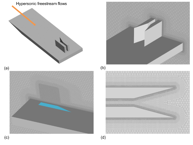
Figure 2: Computational geometry and mesh sketch for the double-fin simulations: (a) the overview of the computational geometry; (b,c,d) the zoom-in views of the Voronoi mesh distributions (70M total mesh elements).

4 Results and discussions

In this section, the numerical results from WMLES with the semi-local scaling based damping function (Eq. (9)) are analyzed and compared against the experimental measurements. The predictions of the WMLES using the van Driest scaling (Eq. (8)) will also be assessed. Hereafter, the operator symbol $<{\cdot}>$ denotes the time- and spanwise-average. The main turbulence statistics are collected within a time interval, which is about 11 flow-through times from the fin leading edge to the trailing edge. In the appendix, simulations with additional 8 flow through times averaging interval are presented demonstrating the adequacy of the statistical sample for the main quantities of interest (pressure and heat transfer profiles).

4.1 WMLES with semi-local scaling based damping function

4.1.1 Overall statistics

Fig. 3 shows the time- and spanwise-averaged Mach number contour on a wall-normal plane and the instantaneous streamwise velocity distribution on a wall-parallel plane at $y/L_{r}=0.3616$ between the leading edge of the flat plate and that of the double fins. A weak shockwave is generated at the leading edge of the flat plate, and slightly decreases the Mach number downstream as shown in Fig. 3(a). The instantaneous streamwise velocity field in Fig. 3(b) shows that the boundary layer transitions, and eventually becomes fully turbulent ahead of the double fins. The turbulent boundary layer appears sustained for approximately $25\delta_{0}$ upstream of the double finned entrance. More quantitative comparisons of the flow statistics between the experimental data and the WMLES results at $x/L_{r}=162$, just upstream of the fins, are given in Fig. 4. While all the statistics close to the boundary layer edge are in good agreement, there are notable discrepancies inside the boundary layer. The discrepancies are in part due to the lingering effect of artificial inflow conditions and relatively short developing length of the incoming boundary layer from the sharp leading edge of the plate. Since the detailed boundary layer statistics between the flat plate leading edge and the fin entrance are unavailable from the experiment, the pursuit of an exact match of all flow profiles between WMLES and experiment at $x/L_{r}=162$ is not realistic. However, as discussed earlier, the flow inside the inlet geometry (between the fins which has been subjected to considerable distortion) may not be as sensitive to the details of the boundary layer flow at the entrance.

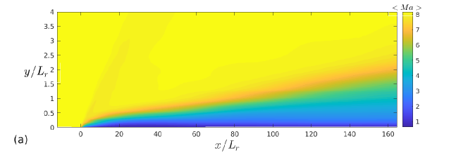
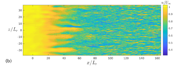
Figure 3: (a) Time- and spanwise-averaged Mach number contour on the wall-normal x-y plane and (b) the instantaneous streamwise velocity distribution on the wall-parallel x-z plane of $y/L_{r}=0.3616$. In panel (b), the high-speed region is associated with the oblique shock wave originating from the leading edge of the flat plate at $x/L_{r}=0$.

The polar plot of the time-averaged profiles of temperature and velocity at $x/L_{r}=162$ is shown in Fig. 5. It is observed that the present WMLES solution agrees with the model prediction of Duan & Martin duan2011direct very well.

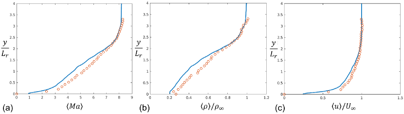
Figure 4: Time- and spanwise-averaged distributions of (a) Mach number, (b) density, and (c) streamwise velocity at $x/L_{r}=162$. The blue lines and the red circles denote the results from WMLES and experiment kussoy1992intersecting , respectively.

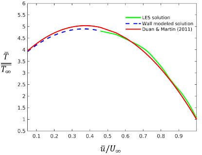
Figure 5: Relation between the time-averaged profiles of temperature and velocity at $x/L_{r}=162$. Also shown is the model prediction from Duan & Martin duan2011direct .

The results of a grid convergence study at $x/L_{r}=162$ is shown in Fig. 6. The fine grid denotes the mesh with parameters given in Table 1. The resolutions of the medium and coarse grids are $50\%$ and $70\%$ coarser than that of the fine grid in each coordinate direction, respectively. The mean streamwise velocity just upstream of the fins exhibits considerable sensitivity to the grid resolution, with profiles from finer grid resolutions moving monotonically closer to the experimental data. In particular, the boundary layer thickness predicted from the medium and coarse grids is $38\%$ smaller than that given by the experiment, and consequently the local effective Reynolds number differs from the experimental setup as well. With the fine grid, the agreement in terms of the boundary layer thickness is good. The mean density profile is less sensitive to grid resolution. Hereafter, only the simulation results from the fine grid will be discussed and compared with the experimental data at downstream locations.

Figure 6: Time- and spanwise-averaged distributions of (a) density and (b) streamwise velocity at $x/L_{r}=162$. The fine grid denotes the mesh with parameters given in Table 1. The resolutions of the medium and coarse grids are $50\%$ and $70\%$ coarser than that of the fine grid in each coordinate direction, respectively. EXP denotes the experimental data kussoy1992intersecting .

Fig. 7 shows the time-averaged $y^{+}$ at the first off-wall cell centers, i.e. the matching locations for the wall model. The largest $y^{+}$ appears around the leading edges of the double fins and the regions where the shock waves impinge on the surfaces. It is noticed that, in the regions upstream of the double-fin entrance, the height of the matching location in plus unit is less than $10$. For the downstream regions where shock/boundary layer interaction occurs, the near-wall eddies and the viscous sublayer are not directly resolved in the simulations and the wall model plays a pivotal role in the predicted flow states.

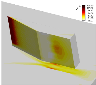
Figure 7: Distribution of the time-averaged $y^{+}$ at the first off-wall cell centers. For facilitating the presentation, only the data over the flat plate and one vertical fin are shown.

The instantaneous and time-averaged surface heat flux distributions, surface pressure, and surface shear stress distributions are shown in Fig. 8. As shown in Fig. 8(a), the instantaneous surface heat flux fluctuates significantly after the double shockwaves induced by the fin leading edges intersect around the shoulders. As shown in Fig. 8(b)(c)(d), right downstream of the shock waves intersection, the distributions of the time-averaged surface heat flux, surface pressure and surface stress attain local maxima around the centerline of the plate. The peak aerodynamic heating and friction occur around the shock impingement locations on the fin surfaces.

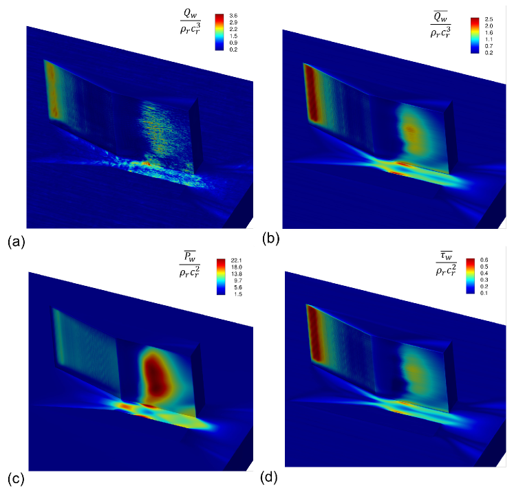
Figure 8: (a) Instantaneous surface heat flux distribution, (b) time-averaged surface heat flux distribution, (c) time-averaged pressure distribution, and (d) time-averaged surface shear stress distribution. The location of the double-shock intersection based on the inviscid theory is around the midpoint of the two fin shoulders. For facilitating the presentation, only the data over the flat plate and one vertical fin are shown.

4.1.2 Data analyses in x-z and x-y planes

The time-averaged surface pressure and heat flux distributions along the centerline of the plate between the two fins as well as the double-shock intersection location based on the inviscid theory are given in Fig. 9. The predicted time-averaged pressure distribution from WMLES is in good agreement with the experiment including in the region downstream of the shocks intersection. The static pressure first increases significantly due to the shockwave intersection and subsequently exhibits a rapid drop due to the expansions emanating from the fin shoulders, as depicted by Fig. 10(a). The peak surface pressure $\overline{P_{w}}/\overline{P_{w,\infty}}\approx 22$ is considerably lower than the prediction from the inviscid theory, $\overline{P_{w}}/\overline{P_{w,\infty}}\approx 45$ gaitonde1995structure . Further downstream at $x/L_{r}\approx 198$, a smaller pressure peak appears due to the second crossing of the reflected shock waves. In terms of the heat flux distribution, the agreement with the experimental data is also favorable across the entire channel between the double fins. The streamwise variation of the surface heat flux follows that of the surface pressure qualitatively. Both the experiment and the WMLES results exhibit an initial decline at $x/L_{r}\approx 170$, and the predicted heat flux is $20\%$ smaller than that from the experiment in the pre-shock region of $x/L_{r}\approx 180$, which is the location of a secondary (small) flow separation (see the discussions of Fig. 12). Downstream of the shock wave intersection, the peak heat flux shows $4\%$ discrepancy between the WMLES results and the experimental data. Similar differences are also observed further downstream at $x/L_{r}=194$ in the low pressure region and heat flux valley (see also Fig. 10). Nevertheless, the present prediction of both quantities shows a much better agreement with the experiment than those from the RANS simulations gaitonde1995structure narayanswami1993numerical . In the RANS solutions, the heat flux plateau around $x/L_{r}=180$ upstream of the shock wave intersection is completely missed. Both the zero-equation Baldwin-Lomax model and the two-equation $k-\epsilon$ model overpredict the peak pressure and the peak heat flux by about $20\%$ (see Fig. 3 and Fig. 9 in narayanswami1993numerical ). As shown in Fig. 10, the predicted nominal shock impingement location on the side fins is around $x/L_{r}=192$ and is similar to the RANS predictions (see Fig. 3 of gaitonde1995structure ).

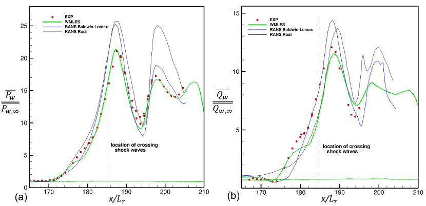
Figure 9: Streamwise distributions of the time-averaged (a) surface pressure and (b) surface heat flux on the flat plate at $z/L_{r}=0$. The green lines and the red dots denote the results from the WMLES simulation and the experiment, respectively. The location of the double-shock intersection based on the inviscid theory is also shown in the plots. Also shown are the results from the zero-equation Baldwin-Lomax model and the two-equation $k-\epsilon$ model narayanswami1993numerical . $\overline{P_{w,\infty}}$ and $\overline{Q_{w,\infty}}$ denote the mean wall pressure and heat flux defined at the location $x/L_{r}=162$, where the so-called “freestream” condition is provided by the experimental report kussoy1992intersecting .

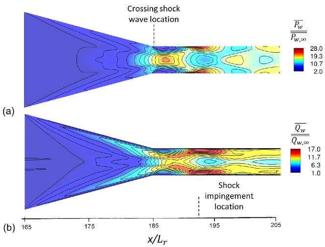
Figure 10: Distributions of the time-averaged (a) surface pressure and (b) surface heat flux on the flat plate at $y/L_{r}=0$. The location of the double-shock intersection based on the inviscid theory is also shown in the plots. Also shown is the shock impingement location around $x/L_{r}=192$.

To characterize the boundary-layer flow separation, Fig. 11 shows the time-averaged surface skin friction lines on the right fin and the corresponding sketch from the experiment. It is observed that the flow separates around the region where the shock wave impinges on the fin surface. While the overall agreement is good, the predicted separation bubble close to the fin surface starts at $x/L_{r}=190$, which is delayed compared to the sketch from the experiment at $x/L_{r}=187$. As summarized in narayanswami1993numerical , the two-equation $k-\epsilon$ model does not capture this separation bubble.

The skin friction lines on the flat plate are given in Fig. 12. The WMLES result is in qualitative agreement with the sketch deduced from experimental measurements, and show similarities with the RANS solution using the Baldwin-Lomax model gaitonde1995structure . There are two lines of coalescence, the principal line of separation (PLS) and the secondary line of separation (SLS). Accordingly, two lines of divergence are also well captured, i.e. the principal line of attachment (PLA) and the center line of attachment (CLA). Close to the centerline, the secondary separation is formed near $x/L_{r}=175$ and characterized by a pair of streamwise counter-rotating vortical structures. The secondary separation continuously shrinks and disappears near $x/L_{r}=197$, where the upside and downside SLS lines converge to the CLA line, i.e. the centerline of the double fins. Fig. 13 shows the zoom-in view of the time-averaged streamlines on the symmetry plane. The maximum height of the secondary separation is roughly $0.5$ cm at $x/L_{r}\approx 178$, which is much smaller than the inlet boundary layer thickness of $3.25$ cm around the leading edge of the double fins, and the predicted flow structure is consistent with that reported in Fig. 11 of gaitonde1995structure .

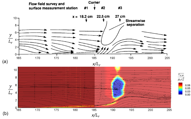
Figure 11: Time-averaged surface skin friction lines on the right fin. Panel (a) denotes the sketch from the experiment and adapted from Fig. 9(b) of kussoy1992intersecting . Panel (b) denotes the present WMLES result and the quantity in the contour represents the time-averaged streamwise skin friction.

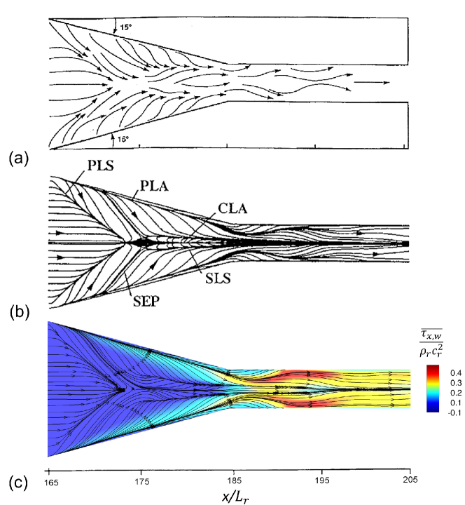
Figure 12: The time-averaged surface skin friction lines on the flat plate. Panel (a) denotes the sketch from the experiment and adapted from Fig. 7(b) of kussoy1992intersecting . Panel (b) denotes the CFD result of RANS approach and adapted from Fig. 9 of gaitonde1995structure . In Panel (b), PLS denotes the principal line of separation, PLA denotes the principal line of attachment, CLA denotes the center line of attachment, SEP denotes the separatrix, and SLS denotes the secondary line of separation. Panel (c) denotes the present WMLES result and the colored contour levels represent the time-averaged streamwise skin friction.

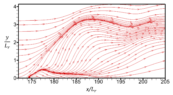
Figure 13: The zoom-in view of the time-averaged streamlines on the symmetry plane. Around $x/L_{r}\approx 174.5$, there is a critical stagnation point located very close to the plate.

The near-wall root-mean-square (r.m.s) statistics of the pressure, temperature and streamwise velocity are given in Fig. 14. The near-wall peak temperature and streamwise velocity fluctuations mainly occur around the secondary lines of separation, in particular at the location where the shockwaves intersect. On the other hand, the peak pressure fluctuations occur on the fin surfaces.

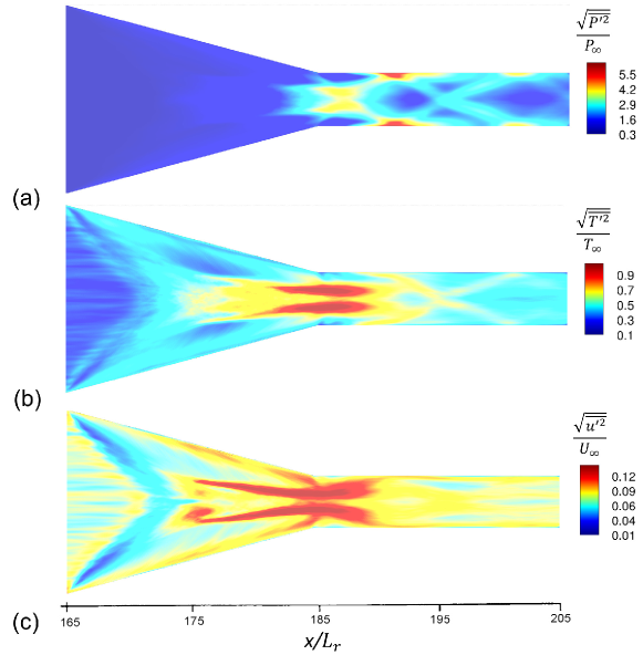
Figure 14: r.m.s statistics of the (a) pressure, (b) temperature and (c) streamwise velocity fluctuations. These statistics are projected to the plate surface from the first off-wall cell centers.

The distributions of the time-averaged wall-normal turbulent heat flux and Reynolds shear stress in the central wall-normal plane are plotted in Fig. 15. The magnitudes of both quantities grow rapidly at the onset of flow separation at $x/L_{r}=175$, and are further amplified by the shock intersection around $x/L_{r}=185$. The spatial structures of the average heat flux and Reynolds shear stress are very similar owing to the strong correlation of temperature and streamwise velocity fluctuations (and manifested in the Reynolds Analogy). Both correlations display layered structures with sign reversals. The impact of this layered distribution on the time-averaged temperature distribution will be discussed in the next section.

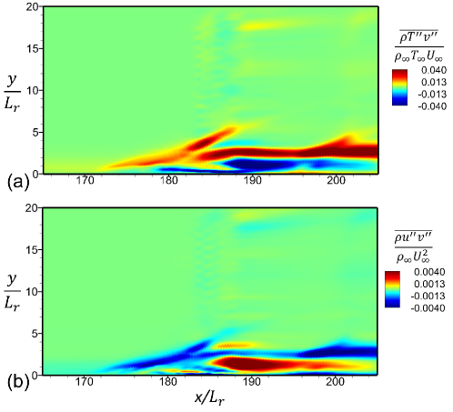
Figure 15: Distributions of (a) the time-averaged wall-normal turbulent heat flux and (b) the time-averaged Reynolds stress on the central wall-normal x-y plane of $z/L_{r}=0$.

4.1.3 Data analyses in y-z planes

The spanwise distributions of the time-averaged surface pressure and surface heat flux at different streamwise stations are given in Fig. 16 and Fig. 17, respectively. Considering the reported $10\%$ uncertainties in the experimental data, the spanwise profiles of both quantities are well captured by the present WMLES for all the considered streamwise stations. The time-averaged pressure profile, deviates noticeably from the experimental measurements in the region $1.2\leq z/L_{r}\leq 2.7$ at station $x/L_{r}=183.2$ before the shock intersection. The agreement is good at the two further downstream stations. The heat flux distributions are in good agreement with the experimental data and superior to those of RANS predictions. In narayanswami1993numerical , it is reported that the peak heat transfer in both RANS computations is overestimated by $50\%$ to $75\%$.

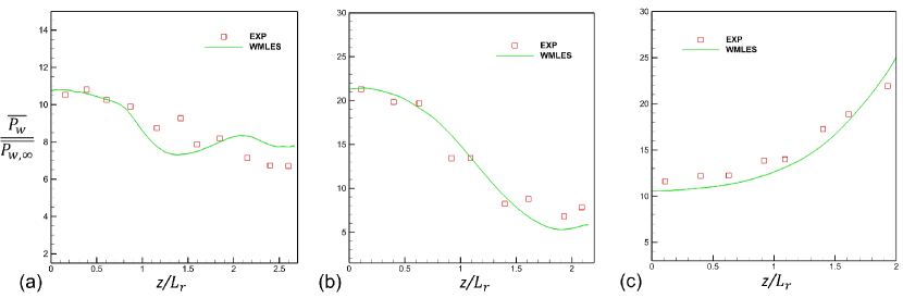
Figure 16: Spanwise distributions of the time-averaged wall pressure $\overline{P_{w}}/\overline{P_{w,\infty}}$ at the streamwise stations: (a) $x/L_{r}=183.2$, (b) $187.5$ and (c) $192$. The experimental data (denoted as EXP) are adapted from the Table 4 of kussoy1992intersecting .

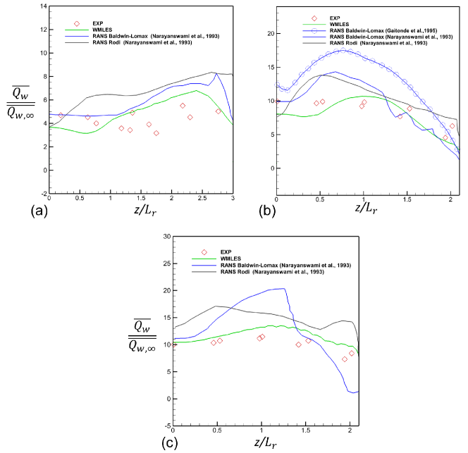
Figure 17: Spanwise distributions of the time-averaged wall heat flux $\overline{Q_{w}}/\overline{Q_{w,\infty}}$ at the streamwise stations: (a) $x/L_{r}=181.5$, (b) $185.8$ and (c) $190.3$. The experimental data (denoted as EXP) are from the Table 4 of kussoy1992intersecting . In panel (b), the RANS result is computed from the Baldwin-Lomax model with grid E - IB, which is elaborated in Fig. 6 of gaitonde1995structure . For all three panels, the RANS predictions in narayanswami1993numerical with the zero-equation Baldwin-Lomax model and the two-equation $k-\epsilon$ (Rodi) model are also shown for comparisons. The locations of the spanwise measurements of the surface heat flux are not coincident with those of the surface pressure in Fig. 16.

Similar to previous investigations of the crossing shock interaction narayanswami1993investigation gaitonde1995structure narayanswami1993numerical , due to the principal and secondary flow separation analyzed in Fig. 12, the salient feature of the streamline structure is a low total pressure region, accompanied by the primary vortex pair close to the center plane, as shown in Fig. 18.

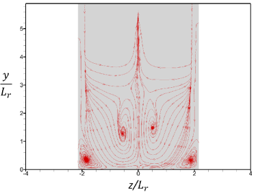
Figure 18: The sectional streamlines on a transverse y-z plane at the streamwise station $x/L_{r}=187.5$.

Fig. 19 shows the total pressure contours on the transverse y-z planes at the pre-shock station, $x/L_{r}=183.2$, the peak pressure station, $x/L_{r}=187.5$, and the further downstream station, $x/L_{r}=192$, respectively. The low total pressure regions are associated with the primary vortex comprising two helical counter-rotating vortices as shown in Fig. 18. At all the considered streamwise stations, the predicted flow structures are qualitatively similar with those from the experiments. The agreement with the experimental data improves in the post-shock intersection regions, where the influences of inflow conditions are less perceptible. For example, as can be seen in Fig. 19(a,b), the total pressure contours from WMLES at $y/L_{r}\leq 3$ have a triangular shape in contrast to the round shape from the experiment at the pre-shock station. This discrepancy (and the effect of inflow conditions) in the pre-shock region is reduced with grid refinement (see Appendix).

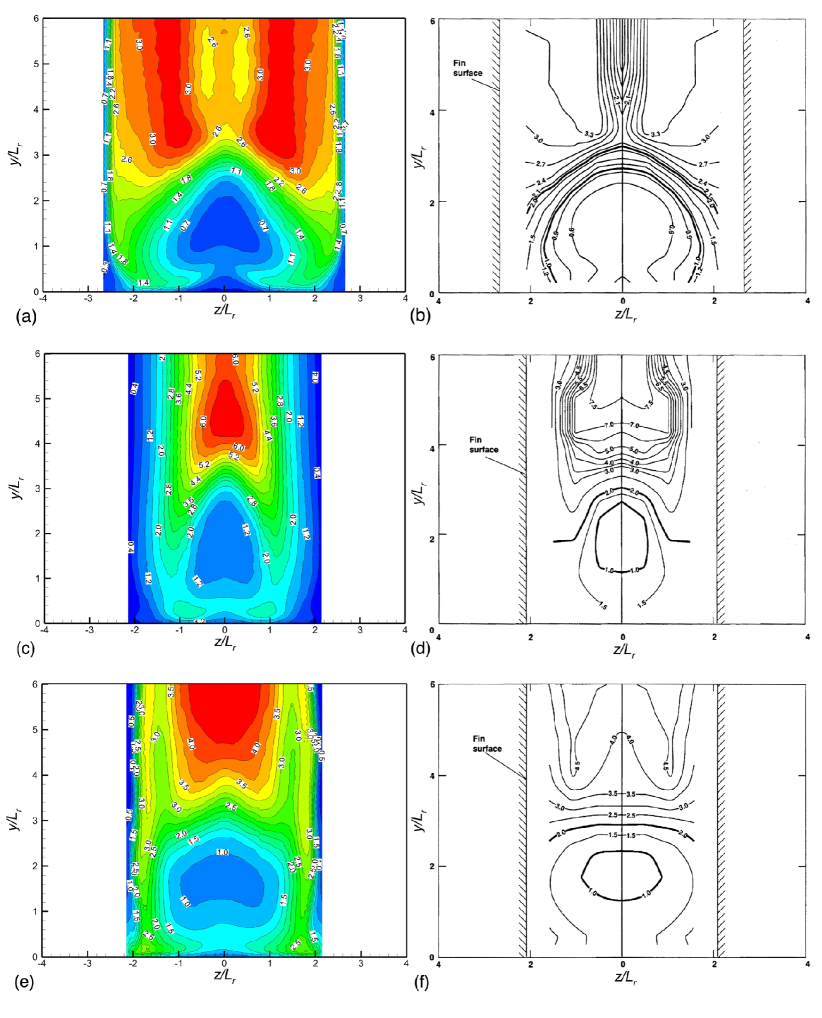
Figure 19: Distribution of the total pressure $\overline{P_{\circ}}/\overline{P_{\circ,\infty}}$ on a transverse y-z plane at $x/L_{r}=183.2$ (a,b), $187.5$ (c,d), and $192$ (e,f). Right panels denote the experimental results adapted from Fig. 11 of kussoy1992intersecting .

Fig. 20 shows the distributions of the time-averaged temperature, r.m.s temperature fluctuations, and r.m.s streamwise velocity fluctuations at $x/L_{r}=183.2$, $187.5$, and $192$. All the quantities shown peak along the central region between the fins. The peak mean temperature is reached away from the flat plate and in the shock intersection region where the velocity and temperature fluctuations are suppressed. As the flow develops further downstream, regions of higher mean temperature and intense velocity and temperature fluctuations move closer to the fins.

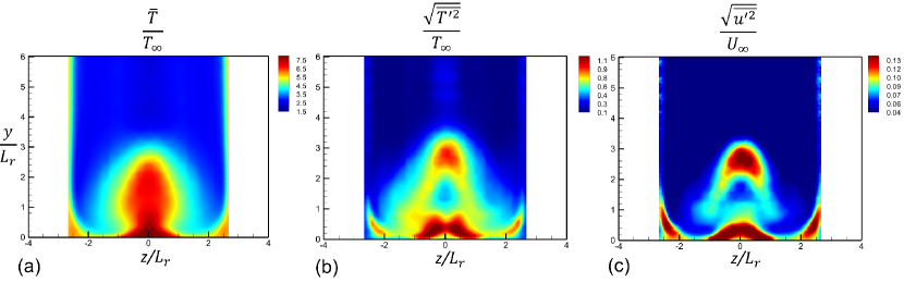
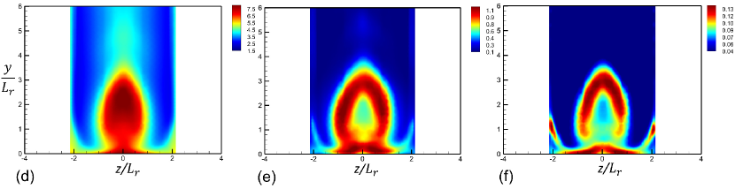
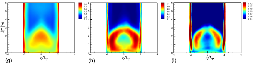
Figure 20: Distributions of the time-averaged temperature (a,d,g), the r.m.s temperature fluctuations (b,e,h), and the r.m.s streamwise velocity fluctuations (c,f,i) on the transverse y-z planes at the streamwise stations with $x/L_{r}=183.2$ (a,b,c), $187.5$ (d,e,f), and $192$ (g,h,i).

Fig. 21 shows the time-averaged turbulent heat flux and Reynolds stress on the transverse y-z planes at three streamwise stations. Once again, a strong correlation between the Reynolds shear stress and heat flux is apparent. Knowledge of the spatial structure of these correlations is valuable in RANS turbulence modeling, where both correlations are phenomenologically modeled in the governing equations for the mean velocity and temperature. The sign reversals of heat flux (and Reynolds stress) in the transverse planes displayed are a consequence of the streamwise vortices and flow reversals owing to the intersecting shocks. The predicted flow fields are marginally asymmetric mainly due to the staggered nature of the deployed unstructured Voronoi mesh and the coarse resolution. Particularly for the downstream unsteady regions, the flow symmetry is more sensitive to the mesh topology. Note that the mean velocity and temperature profiles, and normal components of turbulent intensities are nearly symmetric, but the cross correlations may require much longer time averaging and are apparently more susceptible to asymmetries in the unstructured mesh.

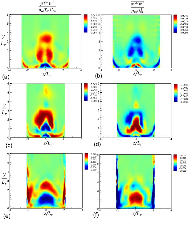
Figure 21: Distributions of the time-averaged wall-normal turbulent heat flux (a,c,e), and the time-averaged Reynolds stress (b,d,f) on the transverse y-z planes at the streamwise station $x/L_{r}=183.2$ (a,b), $187.5$ (c,d), and $192$ (e,f).

4.2 WMLES with van Driest scaling based damping function

In this section, the sensitivity of the results to the coordinate scaling of the wall model eddy viscosity is further evaluated. Wall modeled LES calculations on the “fine” grid using identical freestream boundary conditions described above were additionally performed using the van Driest damping function kawai2012wall . Comparison of the time-averaged pressure and heat flux distributions between the WMLES with the van Driest scaling and semi-local scaling is provided in Fig. 22 and Fig. 23. For all the concerned quantities, the accuracy of the WMLES deteriorates when the van Driest scaling is deployed in the damping function in the eddy viscosity model. In particular, both the mean pressure and heat flux are notably over-predicted near the entrance of the double fins. Distributions of both quantities are also poorly captured after the shock intersection. Comparisons of the spanwise profiles of average pressure and surface heat flux with the experimental data also show higher accuracy with the semi-local scaling.

As shown in Fig. 24, the structure of wall pressure distribution is significantly different from that with semi-local scaling in Fig. 10(a).

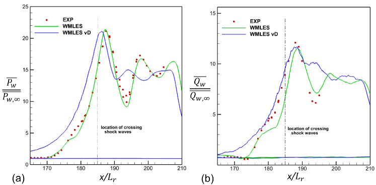
Figure 22: Streamwise distributions of the time-averaged (a) surface pressure and (b) surface heat flux on the flat plate at $z/L_{r}=0$. The green lines, the blue lines and the red symbols denote the data from the WMLES with the semi-local scaling, the WMLES with van Driest scaling, and the experiment, respectively.

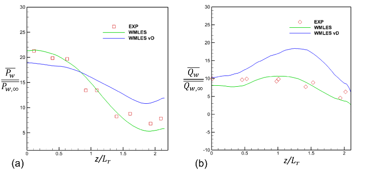
Figure 23: Spanwise distributions of (a) the time-averaged surface pressure at the streamwise station $x/L_{r}=187.5$ and (b) the time-averaged surface heat flux at the streamwise station $x/L_{r}=185.8$. The green lines, the blue lines and the red symbols denote the data from the WMLES with the semi-local scaling, the WMLES with the van Driest scaling, and the experiment, respectively.

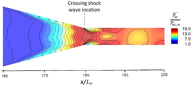
Figure 24: Distribution of the time-averaged pressure on the flat-plate surface at $y/L_{r}=0$. The location of the double-shock intersection based on the inviscid theory is also shown in the plot. The result reported in this plot is from WMLES with van Driest scaling based damping function.

In Fig. 25, the surface heat flux distributions predicted with WMLES with the semi-local scaling and the van Driest scaling are compared. The notable differences present around the centerline secondary separation, the fin corner regions, and the regions right downstream of the shock intersection. The secondary separation is not well captured by the van Driest scaling, which can also be confirmed in Fig. 22(b), where the plateau is missed around $x/L_{r}=180$. In the fin corner regions around $x/L_{r}=185$, where the expansion dominates, the surface heat flux is significantly overpredicted when compared to the semi-local scaling. Downstream of the shock intersection, the valley in the heat flux is also missed by the van Driest scaling.

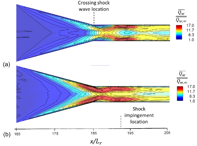
Figure 25: Distributions of the time-averaged surface heat flux from WMLES with (a) the semi-local scaling and (b) the van Driest scaling on the flat plate at $y/L_{r}=0$. The location of the double-shock intersection based on the inviscid theory is shown in the plots. Also shown is the shock impingement location around $x/L_{r}=192$.

5 Conclusions

In this study, an experimentally well documented hypersonic inlet flow involving complex three-dimensional intersecting shock-wave/turbulent boundary-layer interaction and flow separation, is investigated using wall modeled large eddy simulation. Despite the presence of complex non-equilibrium phenomena, the results from WMLES with equilibrium wall model (also with the low-dissipation numerical method and the high-quality Voronoi mesh in the charLES solver) agree favorably with experimental data for mechanical loading, surface heat fluxes, and for the prediction of the secondary separation in both the shock intersection and post-shock regimes. The use of the semi-local scaling in the eddy viscosity of the wall model leads to significant improvements in the results compared to the van Driest scaling. The WMLES predictions are shown to be significantly more accurate than those of prior RANS calculations using either Baldwin-Lomax or $k-\epsilon$ models. The coarseness of the WMLES calculations (relative to the boundary layer thickness or size of the separation bubble) suggest that this approach (which consists of a unique combination of accurate numerical methodology and LES) can be affordable for high speed aerodynamics simulations in geometries of engineering interest.

Data availability

The data that support the findings of this study are available on request from the corresponding author, LF.

Appendix A. Statistical and grid convergence

In this section, the statistical and grid convergence of the main quantities of interest are investigated.

A1. Averaging time convergence study

As shown in Fig. 26, increasing the time averaging interval by 8 flow through times does not affect the pressure and mean surface heat flux statistics, and hence these key quantities of practical interest are considered statistically converged.

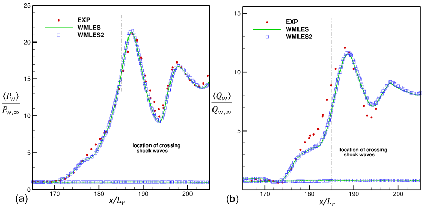
Figure 26: Streamwise distributions of the time-averaged (a) surface pressure and (b) surface heat flux on the flat plate at $z/L_{r}=0$. WMLES denotes the result reported in Fig. 9 and WMLES2 denotes the solution averaged in a time interval, which is 8 flow-through times longer than that of WMLES.

A2. Resolution sensitivity study

A higher-resolution simulation with 143M cells was carried out. This mesh is generated by refining the near-wall region of the mesh with 70M cells (as described in Table 1). As shown in Fig. 27, the results from both resolutions are generally within the experimental uncertainty bars of measured wall pressure. The heat flux predictions upstream of $x/L_{r}=190$ are improved with the finer mesh. In terms of the flow structure, as shown in Fig. 28, the shape of the predicted separation bubble from the higher resolution agrees with the experimental sketch better. Further mesh refinements, especially in the vicinity of the separation bubble may improve the predictions. However, given the intrinsic uncertainties in the prescription of inflow conditions, and the higher cost of more refined computations, we did not carry out additional simulations with finer grid resolution. As remarked earlier, the LES results are always going to be grid dependent, but do converge to DNS in the limit of very fine grids. Here, we have demonstrated the level of accuracy that can be expected at affordable cost.

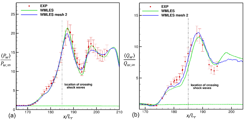
Figure 27: Streamwise distributions of the time-averaged (a) surface pressure and (b) surface heat flux on the flat plate at $z/L_{r}=0$. The results from WMLES with 70M cells and WMLES mesh 2 with 143M cells are reported for comparisons. Also plotted are the uncertainty bars reported from the experiment.

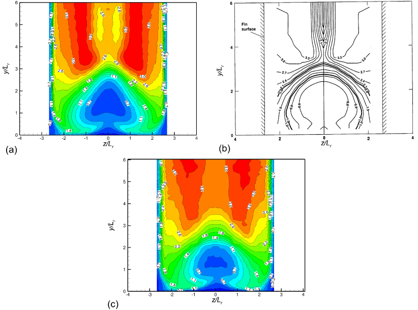
Figure 28: Distribution of the total pressure $\overline{P_{\circ}}/\overline{P_{\circ,\infty}}$ on a transverse y-z plane at $x/L_{r}=183.2$. Panel (b) denotes the experimental result and is adapted from the Fig. 11(a) of kussoy1992intersecting . Panel (a) and (c) denote the WMLES results from the mesh with 70M cells and 143M cells, respectively.

References

- (1) Adams, N.A.: Direct simulation of the turbulent boundary layer along a compression ramp at =3 and = 1685. Journal of Fluid Mechanics 420, 47–83 (2000)
- (2) Aurenhammer, F.: Voronoi diagrams–a survey of a fundamental geometric data structure. ACM Computing Surveys (CSUR) 23(3), 345–405 (1991)
- (3) Baldwin, B., Lomax, H.: Thin-layer approximation and algebraic model for separated turbulentflows. In: 16th aerospace sciences meeting, p. 257 (1978)
- (4) Bermejo-Moreno, I., Campo, L., Larsson, J., Bodart, J., Helmer, D., Eaton, J.K.: Confinement effects in shock wave/turbulent boundary layer interactions through wall-modelled large-eddy simulations. Journal of Fluid Mechanics 758, 5–62 (2014)
- (5) Bose, S.T., Park, G.I.: Wall-modeled large-eddy simulation for complex turbulent flows. Annual Review of Fluid Mechanics 50, 535–561 (2018)
- (6) Bres, G.A., Bose, S.T., Emory, M., Ham, F.E., Schmidt, O.T., Rigas, G., Colonius, T.: Large-eddy simulations of co-annular turbulent jet using a Voronoi-based mesh generation framework. In: 2018 AIAA/CEAS Aeroacoustics Conference, p. 3302 (2018)
- (7) Brès, G.A., Lele, S.K.: Modelling of jet noise: a perspective from large-eddy simulations. Philosophical Transactions of the Royal Society A 377(2159), 20190081 (2019)
- (8) Choi, H., Moin, P.: Grid-point requirements for large eddy simulation: Chapman’s estimates revisited. Physics of fluids 24(1), 011702 (2012)
- (9) Currao, G.M., Choudhury, R., Gai, S.L., Neely, A.J., Buttsworth, D.R.: Hypersonic Transitional Shock-Wave–Boundary-Layer Interaction on a Flat Plate. AIAA Journal pp. 1–16 (2019)
- (10) Duan, L., Beekman, I., Martin, M.P.: Direct numerical simulation of hypersonic turbulent boundary layers. Part 3. Effect of Mach number. Journal of Fluid Mechanics 672, 245–267 (2011)
- (11) Duan, L., Martin, M.: Direct numerical simulation of hypersonic turbulent boundary layers. Part 4. Effect of high enthalpy. Journal of Fluid Mechanics 684, 25 (2011)
- (12) Fu, L., Karp, M., Bose, S.T., Moin, P., Urzay, J.: Shock-induced heating and transition to turbulence in a hypersonic boundary layer. Journal of Fluid Mechanics 909, A8 (2021)
- (13) Fu, S., Wang, L.: RANS modeling of high-speed aerodynamic flow transition with consideration of stability theory. Progress in Aerospace Sciences 58, 36–59 (2013)
- (14) Gaitonde, D., Shang, J.: Calculations on a double-fin turbulent interaction at high speed. In: 11th Applied Aerodynamics Conference, pp. AIAA–93–3432–CP (1993)
- (15) Gaitonde, D., Shang, J., Visbal, M.: Structure of a double-fin turbulent interaction at high speed. AIAA journal 33(2), 193–200 (1995)
- (16) Georgiadis, N.J., Yoder, D.A., Vyas, M.A., Engblom, W.A.: Status of turbulence modeling for hypersonic propulsion flowpaths. Theoretical and Computational Fluid Dynamics 28(3), 295–318 (2014)
- (17) Gottlieb, S., Shu, C.W., Tadmor, E.: Strong stability-preserving high-order time discretization methods. SIAM review 43(1), 89–112 (2001)
- (18) Hader, C., Fasel, H.F.: Direct numerical simulations of hypersonic boundary-layer transition for a flared cone: fundamental breakdown. Journal of Fluid Mechanics 869, 341–384 (2019)
- (19) Helmer, D., Campo, L., Eaton, J.: Three-dimensional features of a Mach 2.1 shock/boundary layer interaction. Experiments in fluids 53(5), 1347–1368 (2012)
- (20) Huang, J., Bretzke, J.V., Duan, L.: Assessment of Turbulence Models in a Hypersonic Cold-Wall Turbulent Boundary Layer. Fluids 4(1), 37 (2019)
- (21) Huang, P., Coleman, G., Bradshaw, P.: Compressible turbulent channel flows: DNS results and modelling. Journal of Fluid Mechanics 305, 185–218 (1995)
- (22) Iyer, P.S., Malik, M.R.: Analysis of the equilibrium wall model for high-speed turbulent flows. Physical Review Fluids 4(7), 074604 (2019)
- (23) Kawai, S., Larsson, J.: Wall-modeling in large eddy simulation: Length scales, grid resolution, and accuracy. Physics of Fluids 24(1), 015105 (2012)
- (24) Kawai, S., Larsson, J.: Dynamic non-equilibrium wall-modeling for large eddy simulation at high reynolds numbers. Physics of Fluids 25(1), 015105 (2013)
- (25) Kussoy, M., Horstman, K.: Intersecting shock-wave/turbulent boundary-layer interactions at Mach 8.3. NASA Ames Research Center Technical Report, NASA-TM-103909 (1992)
- (26) Lakebrink, M.T., Mani, M., Rolfe, E.N., Spyropoulos, J.T., Philips, D.A., Bose, S.T., Mace, J.L.: Toward improved turbulence-modeling techniques for internal-flow applications. AIAA Paper 2019-3703 (2019)
- (27) Larsson, J., Kawai, S., Bodart, J., Bermejo-Moreno, I.: Large eddy simulation with modeled wall-stress: recent progress and future directions. Mechanical Engineering Reviews 3(1), 15–00418 (2016)
- (28) Lehmkuhl, O., Park, G.I., Bose, S.T., Moin, P.: Large-eddy simulation of practical aeronautical flows at stall conditions. Proceedings of the 2018 Summer Program, Center for Turbulence Research, Stanford University pp. 87–96 (2018)
- (29) Lozano-Durán, A., Bose, S.T., Moin, P.: Prediction of trailing edge separation on the NASA Juncture Flow using wall-modeled LES. AIAA Paper 2020-1776 (2020)
- (30) Mani, A., Larsson, J., Moin, P.: Suitability of artificial bulk viscosity for large-eddy simulation of turbulent flows with shocks. Journal of Computational Physics 228(19), 7368–7374 (2009)
- (31) Mettu, B.R., Subbareddy, P.K.: Wall modeled LES of compressible flows at non-equilibrium conditions. AIAA Paper 2018-3405 (2018)
- (32) Muto, D., Daimon, Y., Shimizu, T., Negishi, H.: An equilibrium wall model for reacting turbulent flows with heat transfer. International Journal of Heat and Mass Transfer 141, 1187–1195 (2019)
- (33) Narayanswami, N., Horstman, C., Knight, D.: Numerical Simulation of Crossing Shock/turbulent Boundary Layer Interaction at Mach 8.3: Comparison of Zero and Two-equation Turbulence Models. AIAA paper 93-0779 (1993)
- (34) Narayanswami, N., Knight, D., Horstman, C.: Investigation of a hypersonic crossing shock wave/turbulent boundary layer interaction. Shock Waves 3(1), 35–48 (1993)
- (35) Patel, A., Peeters, J.W., Boersma, B.J., Pecnik, R.: Semi-local scaling and turbulence modulation in variable property turbulent channel flows. Physics of Fluids 27(9), 095101 (2015)
- (36) Rumsey, C.L.: Compressibility considerations for kw turbulence models in hypersonic boundary-layer applications. Journal of Spacecraft and Rockets 47(1), 11–20 (2010)
- (37) Sandham, N., Schülein, E., Wagner, A., Willems, S., Steelant, J.: Transitional shock-wave/boundary-layer interactions in hypersonic flow. Journal of Fluid Mechanics 752, 349–382 (2014)
- (38) Souverein, L.J., Dupont, P., Debieve, J.F., Dussauge, J.P., Van Oudheusden, B.W., Scarano, F.: Effect of interaction strength on unsteadiness in shock-wave-induced separations. AIAA journal 48(7), 1480–1493 (2010)
- (39) Vreman, A.: An eddy-viscosity subgrid-scale model for turbulent shear flow: Algebraic theory and applications. Physics of Fluids 16(10), 3670–3681 (2004)
- (40) Wang, M., Moin, P.: Dynamic wall modeling for large-eddy simulation of complex turbulent flows. Physics of Fluids 14(7), 2043–2051 (2002)
- (41) Wu, X.: Inflow turbulence generation methods. Annual Review of Fluid Mechanics 49, 23–49 (2017)
- (42) Yang, X., Urzay, J., Bose, S., Moin, P.: Aerodynamic heating in wall-modeled large-eddy simulation of high-speed flows. AIAA Journal pp. 731–742 (2017)
- (43) Yang, X.I., Lv, Y.: A semi-locally scaled eddy viscosity formulation for LES wall models and flows at high speeds. Theoretical and Computational Fluid Dynamics 32(5), 617–627 (2018)