NV-Diamond Magnetic Microscopy using a Double Quantum 4-Ramsey Protocol

Abstract

We introduce a double quantum (DQ) 4-Ramsey measurement protocol that enables wide-field magnetic imaging using nitrogen vacancy (NV) centers in diamond, with enhanced homogeneity of the magnetic sensitivity relative to conventional single quantum (SQ) techniques. The DQ 4-Ramsey protocol employs microwave-phase alternation across four consecutive Ramsey (4-Ramsey) measurements to isolate the desired DQ magnetic signal from any residual SQ signal induced by microwave pulse errors. In a demonstration experiment employing a 1-$\upmu$m-thick NV layer in a macroscopic diamond chip, the DQ 4-Ramsey protocol provides volume-normalized DC magnetic sensitivity of $\eta^{\text{V}}=34\,$nT Hz${}^{-1/2}\,\upmu$m^3/2 across a $125\text{\,}\mathrm{\SIUnitSymbolMicro m}$$\times$$125\text{\,}\mathrm{\SIUnitSymbolMicro m}$ field of view, with about 5$\times$ less spatial variation in sensitivity across the field of view compared to a SQ measurement. The improved robustness and magnetic sensitivity homogeneity of the DQ 4-Ramsey protocol enable imaging of dynamic, broadband magnetic sources such as integrated circuits and electrically-active cells.

I Introduction

Nitrogen-vacancy (NV) color centers in diamond constitute a leading quantum sensing platform, with particularly diverse applications in magnetometry [1]. The negatively-charged NV${}^{\text{-}}$ center has an electronic spin-triplet ground state with magnetically-sensitive spin resonances, offers all-optical spin-state preparation and readout under ambient conditions, and can be engineered at suitably high densities in favorable geometries [2, 3]. These properties make ensembles of NV${}^{\text{-}}$ centers particularly advantageous for wide-field magnetic microscopy of physical and biological systems with micrometer-scale spatial resolution, a modality known as the quantum diamond microscope (QDM) [4]. QDM applications to date include imaging magnetic fields from remnant magnetization in geological specimens [5], domains in magnetic memory [6], iron mineralization in chiton teeth [7], current flow in graphene devices [8, 9] and integrated circuits [10], populations of living magnetotactic bacteria [11], and cultures of immunomagnetically labeled tumor cells [12].

Despite this progress, QDM magnetic imaging applications have been largely restricted to mapping of static magnetic fields exceeding several microtesla due to shortcomings of conventional single quantum (SQ) magnetometry. SQ schemes sense changes in the frequency or phase accumulation between two sublevels with difference in spin projection quantum number $\Delta m=1$. In particular, the sensitivity of QDMs using continuous-wave optically detected magnetic resonance (CW-ODMR) is impaired by competing effects of the optical and microwave (MW) control fields applied during the sensing interval [4, 3]. Pulsed-ODMR schemes, which separate the optical spin-state preparation and readout from the MW control and sensing interval, offer improved sensitivity, but cannot exceed the performance achievable with SQ Ramsey magnetometry [3].

Furthermore, any SQ magnetometry scheme is vulnerable to diamond crystal stress inhomogeneities and temperature variations, which shift and broaden the NV${}^{\text{-}}$ spin resonances. Such stress gradients are particularly pernicious for QDM applications, with typical gradient magnitudes comparable to NV${}^{\text{-}}$ resonance linewidths ($0.1\!-\!1\,$MHz) and spatial structure spanning the submicron to millimeter scales [13]. Stress-induced resonance shifts or broadening may be mistaken for magnetic signals of interest. Stress gradients can also degrade per-pixel sensitivity and sensitivity homogeneity across an image. While protocols such as sequentially sampling the ODMR spectrum at multiple frequencies [5] or employing four-tone MW control [14, 15] can separate magnetic and non-magnetic signals, the worsened and inhomogeneous magnetic sensitivity caused by stress gradients remains unaddressed.

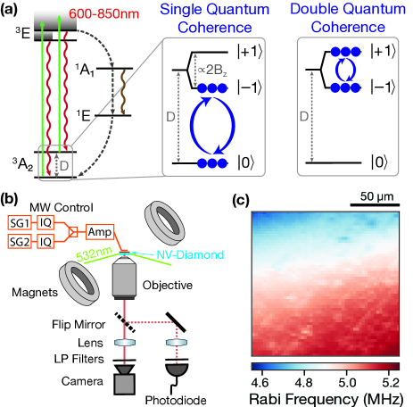
Figure 1: The NV${}^{\text{-}}$ Energy Level Diagram and Experimental Apparatus. (a) Energy level diagram for the negatively-charged nitrogen vacancy (NV${}^{\text{-}}$) in diamond with zero field splitting $D$ between the ground state spin levels $|m_{s}\!=\!0\rangle$ and $|m_{s}=\!\pm\!1\rangle$. The enlarged views depict single quantum (SQ) and double quantum (DQ) coherence. To induce a DQ coherence, the $|0\rangle\!\rightarrow\!|\pm 1\rangle$ spin transitions are simultaneously irradiated with a two-tone resonant microwave (MW) pulse. (b) An overview of the QDM apparatus including $532\text{\,}\mathrm{n}\mathrm{m}$ excitation of a micron-scale layer of NV centers in a macroscopic diamond chip, using total internal reflection (TIR). NV fluorescence is collected using a 20$\times$ objective onto a camera or photodiode. 647 nm and 532 nm long-pass (LP) optical filters partially isolate NV${}^{\text{-}}$ fluorescence from background NV${}^{\text{0}}$ fluorescence. MW control fields are synthesized using two signal generators with phase control on both tones and applied via a millimeter-scale shorted coaxial loop. A bias magnetic field of $5\text{\,}\mathrm{mT}$ is aligned with NV centers oriented along a single crystallographic axis. (c) Typical NV${}^{\text{-}}$ Rabi frequency variation across a $125\text{\,}\mathrm{\SIUnitSymbolMicro m}$$\times$$125\text{\,}\mathrm{\SIUnitSymbolMicro m}$ field of view. The effects of inhomogeneous, stress-induced NV${}^{\text{-}}$ resonance shifts on the Rabi frequency are visible in addition to a quasi-linear Rabi gradient due to spatial variation in the MW amplitude.

Here, we demonstrate a double quantum (DQ) 4-Ramsey protocol that overcomes the shortcomings of SQ CW- and pulsed-ODMR measurement techniques. This protocol expands upon the advantageous pulsed Ramsey scheme, which temporally separates the spin state control, optical readout, and sensing intervals. The scheme thus enables use of increased laser and MW intensity compared to CW-ODMR, allowing for improved measurement contrast and higher fluorescence count rates without broadening the NV${}^{\text{-}}$ spin resonances. Furthermore, the protocol exploits the benefits of DQ coherence magnetometry, which leverages a double quantum superposition of the $m_{s}=|\pm 1\rangle$ ground-state sublevels, to cancel common-mode resonance shifts and broadening from stress, electric fields, and temperature variations [16, 17, 18, 19]. This DQ Ramsey-based scheme can therefore disentangle magnetic and non-magnetic signals while also enabling improved, homogeneous per-pixel magnetic sensitivity across an image.

Previously, DQ Ramsey magnetic imaging has been hindered by the technical challenge of producing sufficiently uniform and strong MW fields to avoid spatially-varying errors in the optimal MW pulses and hence the NV${}^{\text{-}}$ measurement protocol. Such pulse errors result in residual SQ coherence that remains sensitive to common-mode shifts of the $\ket{\pm 1}$ sublevels, degrading the robustness of DQ magnetometry to stress-induced shifts and temperature drifts.

The present work circumvents this challenge with a DQ 4-Ramsey protocol specifically designed to suppress the contribution of residual SQ coherence. By properly selecting the spin-1 rotations applied in four consecutive Ramsey measurements (4-Ramsey), the DQ signal from each Ramsey measurement is preserved while the residual SQ signals cancel. This scheme is broadly applicable to both NV${}^{\text{-}}$ ensemble imaging and bulk sensing modalities, simultaneously mitigating the pernicious effects of stress-gradients and temperature-induced drifts. Since the 4-Ramsey protocol is a straightforward extension of established phase-alternation schemes, implementation in an existing system does not typically require additional MW components.

After describing the NV${}^{\text{-}}$ center and experimental apparatus in Sec. II, we outline and experimentally demonstrate the DQ 4-Ramsey protocol (Sec. III). In Sec. IV, we use SQ and DQ Ramsey fringe imaging to characterize, pixel by pixel, the reduced spatial variation in $T_{2}^{*}$ and NV${}^{\text{-}}$ resonance frequency when using the DQ sensing basis. Using the same field of view as in Sec. IV, we then measure a $1.5\times$ improved median per-pixel sensitivity and a $4.7\times$ narrower spatial distribution of per-pixel sensitivity using the DQ sensing basis compared to the SQ basis (Sec. V). In Sec. VI we highlight next steps to further improve DC magnetic sensitivity and temporal resolution, and we provide an outlook describing envisioned applications for high-sensitivity, broadband magnetic microscopy using the DQ 4-Ramsey protocol.

II Experimental Methods

The NV center is a $\text{C}_{\text{3v}}$ symmetric color center in diamond formed by substitution of a nitrogen atom adjacent to a vacancy in the carbon lattice. We restrict attention to the negatively charged NV${}^{\text{-}}$ center, which has an electronic spin-triplet ($S=1$) ground state with a zero-field-splitting at room temperature $D\approx 2.87$ GHz between the $|m_{s}=0\rangle$ and $|m_{s}=\pm 1\rangle$ magnetic sublevels as shown in Fig. 1(a). Application of an external magnetic field splits the $|\pm 1\rangle$ sublevels by the Zeeman effect. In the presence of a magnetic field $\vec{B}$ exceeding $\approx$$1\text{\,}\mathrm{mT}$ aligned with the NV${}^{\text{-}}$ symmetry axis $z$, the NV${}^{\text{-}}$ ground-state Hamiltonian can be approximated as [5, 13, 20, 21, 22]:

$$H/h\approx[D(T)+M_{z}]S^{2}_{z}+\frac{\gamma}{2\pi}B_{z}S_{z},$$ (1)

where $S_{z}$ is the dimensionless spin-1 operator, $M_{z}$ is the axial spin-stress coupling parameter, $D(T)$ is the temperature-dependent zero-field-splitting, $B_{z}$ is the projection of the external magnetic field $\vec{B}$ along the NV${}^{\text{-}}$ symmetry axis, and $\gamma/(2\pi)=$$28.03\text{\,}\mathrm{GHz}\text{\,}{\mathrm{T}}^{-1}$ is the NV${}^{\text{-}}$ gyromagnetic ratio. Transverse magnetic, electric, and crystal stress terms are neglected as motivated in Refs. [13, 16, 23] (see the Supplemental Material [24] for further discussion of the crystal stress terms). Under these assumptions, the observed spatial variations in NV${}^{\text{-}}$ resonance frequencies and linewidths are attributed to axial stress gradients arising from stress inhomogeneity in the host diamond crystal. Note that for DQ coherence magnetometry, the relative phase accumulated between the $\ket{\pm 1}$ sublevels is not only immune to common-mode energy level shifts (proportional to $S_{z}^{2}$ in Eq. 1) but also doubly sensitive to magnetic fields [18, 17, 16].

The present study employs a QDM to image spin-state-dependent fluorescence from a 1-$\upmu$-thick nitrogen-doped CVD diamond layer ([$\text{N}_{\text{total}}$]$\,\approx\!20\,$ppm, ${}^{12}\text{C}\!=\!99.995$%, natural abundance nitrogen) grown by Element Six Ltd. on a ($2\times 2\times 0.5$) mm³ high purity diamond substrate. Post-growth treatment via electron irradiation and annealing increased the $\text{NV}^{\text{-}}$ concentration in the nitrogen-doped layer to $\approx\,$2 ppm. The magnitude and distribution of stress inhomogeneity in the selected sample is representative of typical diamonds fabricated for NV-based magnetic imaging (see Refs. [13, 25] for additional examples).

An approximately $150\text{\,}\mathrm{\SIUnitSymbolMicro m}$ by $300\text{\,}\mathrm{\SIUnitSymbolMicro m}$ region of the NV layer is illuminated with $1\text{\,}\mathrm{W}$ of $532\text{\,}\mathrm{nm}$ laser light in a total internal reflection (TIR) geometry [see Fig. 1(b)]; and the associated NV${}^{\text{-}}$ fluorescence is collected onto either a Heliotis heliCam C3 camera or a Hamamatsu C10508 avalanche photodiode. The heliCam operates by subtracting alternate exposures in analog and then digitizing the resultant background-subtracted signal. This procedure enables the detected magnetic-field-dependent NV${}^{\text{-}}$ fluorescence to fill the 10-bit dynamic range of each pixel for modulated magnetometry sequences synchronized with the camera exposures. With an external frame-rate of up to $3.8\text{\,}\mathrm{kHz}$, the heliCam provides submillisecond temporal resolution; while the internal exposure rate of up to $1\text{\,}\mathrm{MHz}$ enables the accumulation of signal from multiple Ramsey measurements, each a few microseconds in duration, per external frame (Supplemental Material [24]). Two signal generators with phase control synthesize the dual-tone MW fields required for DQ coherence magnetometry in the presence of a bias magnetic field (Appendix A). Control over the relative phase between the two MW tones enables selective coupling to different DQ superposition states as described in the following section. These MW fields are applied to the NV${}^{\text{-}}$ ensemble using a millimeter-scale shorted coaxial loop. Figure 1(c) depicts the typical spatial variation in Rabi frequency.

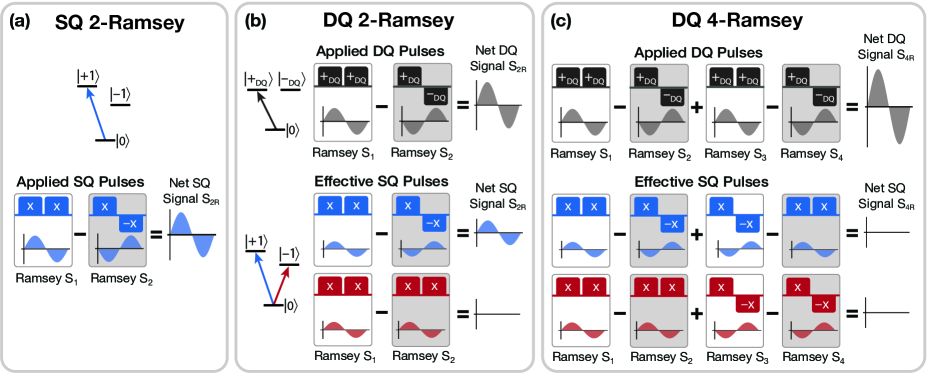
Figure 2: 2-Ramsey and 4-Ramsey Measurement Protocols. (a) Representation of the single quantum (SQ) 2-Ramsey protocol. The choice of phases and resultant DC magnetometry signals are shown for each Ramsey sequence. The single-tone MW pulses address only the $\ket{0}\rightarrow\ket{+1}$ spin resonance. (b) Representation of the double quantum (DQ) 2-Ramsey protocol. In the top row (gray), the two-tone DQ pulses applied during each Ramsey sequence are depicted above the DC magnetometry curve associated with that choice of phases. The net DQ magnetometry signal S${}_{\text{2R}}$ is shown on the right. In the middle and bottom rows, the applied MW pulses are decomposed into effective SQ rotations for each pseudo-two-level system. Note that the SQ signals produced by the effective pulses addressing the $\ket{0}\rightarrow\ket{+1}$ transition (blue) do not cancel. As a result, SQ signals corrupt the resultant DQ 2-Ramsey signal when residual SQ coherence is present. (c) Representation of the DQ 4-Ramsey measurement protocol to cancel residual SQ signals resulting from MW pulse errors. The net DQ magnetometry signal S${}_{\text{4R}}$ is shown on the right. In the presence of pulse errors, the resultant SQ DC magnetometry signals for each Ramsey sequence are depicted and shown to produce no net SQ signal when combined according to Eq. 2.

Figure 3: Measured Response to Common-Mode and Differential Detunings. (a) Depiction of the applied MW field frequencies detuned from the NV${}^{\text{-}}$ resonances in common mode by $\delta_{\text{cm}}$ to emulate stress- and temperature-induced shifts. (b) Single-channel (photodiode) measurements of the NV${}^{\text{-}}$ response to common-mode shifts of the $\ket{0}\rightarrow\ket{-1}$ and $\ket{0}\rightarrow\ket{+1}$ spin resonances. For each sensing protocol, $\delta_{\text{cm}}=0$ indicates the point of maximum slope after calibration (see Appendix B). The SQ 2-Ramsey response, addressing only the $\ket{0}\rightarrow\ket{+1}$ spin resonance, is included for reference. The DQ 4-Ramsey response to common-mode shifts is suppressed by 96$\times$ compared to the SQ 2-Ramsey shift response. (c) Depiction of the applied MW field frequencies detuned from the NV${}^{\text{-}}$ resonances differentially by $\pm\delta_{\text{diff}}$ to emulate axial-magnetic-field-induced shifts. (d) Single-channel measurements of the NV${}^{\text{-}}$ response to differential shifts of the $\ket{0}\rightarrow\ket{-1}$ and $\ket{0}\rightarrow\ket{+1}$ spin resonances. For each measurement protocol, $\delta_{\text{diff}}=0$ indicates the point of maximum slope after calibration, which determines the optimal magnetometer sensitivity. The SQ 2-Ramsey response, addressing only the $\ket{0}\rightarrow\ket{+1}$ spin resonance, is included for reference.

III DQ 4-Ramsey Measurement Protocol

We introduce a measurement protocol consisting of four consecutive Ramsey sequences that, when combined, isolate the desired DQ magnetometry signal from residual SQ signal by modulating the MW pulse phases. SQ protocols commonly employ sets of two Ramsey sequences (2-Ramsey), alternating the phase of the final $\pi$/2 pulse in successive sequences by $180^{\circ}$, to modulate the NV${}^{\text{-}}$ fluorescence and cancel low-frequency noise, such as $1/f$ noise [26]. In such a SQ 2-Ramsey protocol, the magnetometry signal alternately maps to positive and negative changes in NV${}^{\text{-}}$ fluorescence, such that subtracting every second detection from the previous yields a rectified magnetometry signal [see Fig. 2(a)].

Analogous DQ 2-Ramsey protocols exist: two-tone MW pulses couple the $\ket{0}$ state to equal-amplitude superpositions of the $\ket{\pm 1}$ states, with a phase relationship $(\ket{+1}+e^{i\Delta\phi}\ket{-1})/2$ determined by the relative phase $\Delta\phi$ between the two MW tones [17]. By modulating $\Delta\phi\!=\!\{$$,$$\}$ between the tones in the final $\pi/2$ pulse, the $\ket{0}$ state can be alternately coupled to the orthogonal superposition states $\ket{\pm\text{DQ}}=(\ket{+1}\pm\ket{-1})/\sqrt{2}$. Figure 2(b) depicts a representative DQ 2-Ramsey protocol.

Although DQ 2-Ramsey protocols effectively cancel noise at frequencies below the phase modulation frequency, this does not disentangle the desired DQ signal from unwanted SQ signal arising from MW pulse errors. In NV${}^{\text{-}}$ ensemble measurements, MW pulse errors commonly arise from spatial gradients in the Rabi frequency across an interrogated ensemble or field of view, see Fig. 1(c) for an example of the typical Rabi gradient for a millimeter-scale shorted coaxial loop. Although the spatial properties of the MW control field depend upon setup-specific MW synthesis and delivery approaches, the 4-Ramsey protocol universally relaxes requirements on MW-field uniformity. The hyperfine splitting of the NV${}^{\text{-}}$ resonances and stress-induced NV${}^{\text{-}}$ resonance shifts can also introduce MW pulse errors via the detuning-dependent effective Rabi frequency. In this work, errors induced by the hyperfine splitting ($2.2\text{\,}\mathrm{MHz}$ between each of the $m_{I}=\{-1,0,+1\}$ ¹⁴N nuclear spin states) are comparable to the Rabi gradient of $\pm\,$200 kHz and uniform across the field of view. In addition, the spatially-correlated Rabi frequency variations on the 1$-$10$\,\upmu$m length scales in Fig. 1(c) are attributed to stress-induced shifts on the order of hundreds of kilohertz (see Sec. IV and Supplemental Material [24]).

We now describe the phase alternation pattern used in the DQ 4-Ramsey protocol to isolate DQ magnetic signals and present an experimental demonstration using photodiode-based measurements. Figure 2(c) depicts the resulting DQ rotations applied in the {$\ket{0}$, $\ket{-\text{DQ}}$, $\ket{+\text{DQ}}$} basis for a particular implementation of the DQ 4-Ramsey protocol, where the choice of relative phases is restricted to $0\mathrm{°}$ or $180\mathrm{°}$ (generalized phase requirements can be found in the Supplemental Material [24]). While the initial pulse in each Ramsey sequence prepares the $\ket{+\text{DQ}}$ state, the final pulse alternately couples to the $\ket{+\text{DQ}}$ and $\ket{-\text{DQ}}$ states, similar to the DQ 2-Ramsey protocol. If the signal from each of the four measurements $i=1\!-\!4$ is denoted by $S_{i}$ then the rectified DQ signal $S_{4R}$ is given by

$$S_{4R}=S_{1}-S_{2}+S_{3}-S_{4}$$ (2)

where, as shown in Fig. 2(c), $S_{2}$ and $S_{4}$ contain DQ signals with opposite sign compared to $S_{1}$ and $S_{3}$. When implementing these DQ rotations, we have flexibility in choosing the absolute phases of each tone. For example, {$0\mathrm{°}$, $0\mathrm{°}$} and {$180\mathrm{°}$, $180\mathrm{°}$} both couple to $\ket{+\text{DQ}}$ while {$0\mathrm{°}$, $180\mathrm{°}$} and {$180\mathrm{°}$, $0\mathrm{°}$} couple to $\ket{-\text{DQ}}$. We leverage this degree of freedom to ensure that residual SQ signals are canceled by Eq. 2. The effective SQ pulses applied to each two-level subsystem transition ($\ket{0}\rightarrow\ket{+1}$ and $\ket{0}\rightarrow\ket{-1}$) are illustrated in Fig. 2(c) as Bloch sphere rotations about the axes $x$ and $-x$.

If pulse errors arise, leading to residual SQ coherence, then the resultant SQ signal contained in the summation $S_{2}$+$S_{4}$ is the same as $S_{1}$+$S_{3}$ (so long as the errors are constant over the $\sim 10\,\mu$s measurement duration). By subtracting these summations, $S_{\text{4R}}$ from Eq. 2 eliminates this spurious SQ signal. When using the heliCam, Eq. 2 is physically implemented by the on-chip circuitry, which subtracts alternating exposures in analog before digitization. For photodiode-based measurements, which provide access to $S_{1-4}$ directly, the right hand side of Eq. 2 can be divided by the sum of $S_{1-4}$ to cancel the effects of multiplicative noise sources such as laser intensity fluctuations.

Figure 3 illustrates the benefit of the DQ 4-Ramsey protocol over SQ and DQ 2-Ramsey protocols. The measured changes in contrast in response to differential (magnetic-field-like) and common-mode (temperature, axial-stress-like) shifts are compared when operating with a free precession interval $\tau$ and detuning from the center hyperfine resonance, optimized for magnetic sensitivity (see Appendix B). For the data presented in Figs. 3, NV${}^{\text{-}}$ fluorescence from the same field of view as shown in Fig. 1(c) is collected onto a photodiode while sweeping the applied MW tone(s). By approximating the change in fluorescence about the optimal detuning ($\delta_{\text{cm}}$ $=$ $\delta_{\text{diff}}$ $=$ $0$) using a linear fit, we find that DQ Ramsey measurements using the conventional 2-Ramsey protocol (with residual SQ signal) suppress the response to common-mode shifts $\delta_{\text{cm}}$ compared to SQ 2-Ramsey measurements by a factor of 7. Although this suppression factor depends on both the particular setup and diamond, the factor of 7 reported in this work is similar to that in Ref. [18] for a single NV${}^{\text{-}}$, which also attributes the residual observed response to MW pulse imperfections. Meanwhile, under the same experimental conditions, the DQ 4-Ramsey protocol suppresses the common shift response by about a factor of 100 compared to SQ Ramsey measurements. The residual DQ 4-Ramsey protocol response to common-mode shifts, visible in the inset of Fig. 3(b), is attributed to experimental imperfections when manipulating the phase of the MW control pulses. Alternative hardware implementations (e.g., using an arbitrary waveform generator) could likely yield further suppression of the DQ 4-Ramsey protocol response to common-mode shifts.

As depicted in Fig. 3(d), the DQ 4-Ramsey and DQ 2-Ramsey responses exhibit about a cumulative 25% increase in slope (and an associated improvement in magnetometer sensitivity) compared to the SQ 2-Ramsey response, after accounting for the increased effective gyromagnetic ratio in the DQ basis and the loss of DQ contrast due to pulse errors. When each Ramsey signal $S_{i}$ is accessible, the bandwidth of the 4-Ramsey measurement is approximately half the bandwidth of the 2-Ramsey measurement. However, there is no corresponding decrease in sensitivity because the acquired DQ magnetic signals add constructively across the 4-Ramsey protocol (see Supplemental Material [24]).

IV Ramsey Fringe Imaging

We employ SQ 2-Ramsey and DQ 4-Ramsey measurements to image the NV${}^{\text{-}}$ ensemble spin properties relevant for DC magnetic field sensitivity across a $125\text{\,}\mathrm{\SIUnitSymbolMicro m}$ by $125\text{\,}\mathrm{\SIUnitSymbolMicro m}$ field of view. The photon-shot-noise-limited sensitivity of a Ramsey-based measurement $\eta_{\text{ramsey}}$ depends upon the NV${}^{\text{-}}$ ensemble dephasing time $T_{2}^{*}$, the contrast $C$, and the average number of photons collected per measurement $N$ [3]:

$$\eta_{\text{ramsey}}=\frac{1}{\gamma}\frac{1}{\Delta m}\frac{1}{Ce^{-(\tau/T_{2}^{*})^{p}}\sqrt{N}}\frac{\sqrt{\tau+t_{r,i}}}{\tau}$$ (3)

where $\Delta m$ accounts for the difference between the $m_{s}$ states used for the sensing basis ($\Delta m\!=\!1,2$ for the SQ, DQ bases), $\tau$ is the free precession interval per measurement, $p$ describes the decay shape, and $t_{r,i}$ indicates the duration of time dedicated to readout and initialization per measurement. The optimal free precession interval is determined by the NV${}^{\text{-}}$ ensemble dephasing time $T_{2}^{*}$, which is proportional to the inverse of the inhomogeneous linewidth $\Gamma$ ($T_{2}^{*}\!=\,$1/$\pi\Gamma$ assuming a Lorentzian lineshape). Axial stress gradients within a pixel degrade $\eta_{\text{ramsey}}$ by decreasing $T_{2}^{*}$; stress-induced resonance shifts across an image both worsen $\eta_{\text{ramsey}}$ by ensuring that the chosen MW frequency is sub-optimal for all but a subset of pixels and introduce spatially-varying, non-magnetic offsets in the Ramsey signal that can complicate data analysis [13].

We image the NV${}^{\text{-}}$ ensemble spin properties by sweeping the free precession time in the SQ and DQ Ramsey sequences and fitting the fringes to a sum of oscillations with a common decay envelope:

$$S_{\text{ramsey}}(\tau)=e^{-\tau/T_{2}^{*}}\sum_{i=m_{I}}A_{i}\sin(2\pi f_{i}+\delta_{i})$$ (4)

where each oscillatory term, indexed by $m_{I}=\{-1,0,1\}$ (for an ${}^{14}\text{N}$ ensemble), has an amplitude $A_{i}$, frequency $f_{i}$, phase shift $\delta_{i}$, and decay shape fixed to $p=1$ [16]. A purposeful detuning of $3\,$MHz from the resonance corresponding to the $m_{I}=0$ hyperfine population was introduced in order to more easily extract all three frequencies and the decay envelope. Eq. 4 was rapidly fit to the data pixel-by-pixel using the open source, GPU-accelerated non-linear least-squares fitting software, GPUfit [27]. The typical 95% confidence intervals (C.I.) for the extracted dephasing times $T_{2}^{*}$ and amplitudes $A_{i}$ discussed below are less than 5%, while the typical C.I. for $f_{i}$ are about 0.5%.

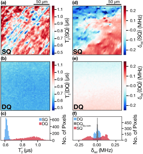
Figure 4: Imaging Ensemble Spin Properties. (a) Image of the single quantum (SQ) $T_{2}^{*}$ extracted by fitting the SQ 2-Ramsey fringe decay to Eq. 4. The field of view is $125\text{\,}\mathrm{\SIUnitSymbolMicro m}$ by $125\text{\,}\mathrm{\SIUnitSymbolMicro m}$. Spatial variations in $T_{2}^{*}${SQ} are due to stress-induced broadening of the NV${}^{\text{-}}$ resonances within the three-dimensional volume imaged onto a pixel. (b) Image of the double quantum $T_{2}^{*}${DQ} measured using the DQ 4-Ramsey protocol across the same field of view as shown in (a). In pixels with minimal stress gradients, the $T_{2}^{*}${DQ} is half the $T_{2}^{*}${SQ}, as expected, due to the effectively doubled dipolar coupling to the surrounding paramagnetic spin bath, which dominates the NV${}^{\text{-}}$ dephasing [16]. (c) Histogram of $T_{2}^{*}${SQ} and $T_{2}^{*}${DQ} values from the pixels in (a) and (b). (d) Image of the relative SQ resonance shifts $\delta_{\text{rel}}${SQ} from the median SQ Ramsey fringe frequency. Variations in $\delta_{\text{rel}}${SQ} are attributed predominantly to axial-stress-induced shifts of the NV${}^{\text{-}}$ resonance frequencies between pixels. (e) Image of the relative DQ detuning $\delta_{\text{rel}}${DQ} across the same field of view as shown in (a, b, d). The axial-stress-induced shifts apparent in (d) are mitigated. Inhomogeneity in the magnitude of the applied bias magnetic field $B_{0}$ results in a residual gradient of less than 1.4$\,\upmu$m. (f) Histogram of the extracted SQ and DQ $\delta_{\text{rel}}$ values from the pixels in (d) and (e). The distribution of DQ $\delta_{\text{rel}}$ values with the setup-specific $B_{0}$-gradient contribution corrected is shown in gray.

Dephasing times – The extracted $T_{2}^{*}$ values for the SQ and DQ sensing bases are shown as images in Fig. 4(a) and 4(b) and plotted as a histogram in Fig. 4(c). To quantify the non-normal spread in $T_{2}^{*}$ values, we report the median value and the relative inter-decile range (RIDR):

$$\sigma_{\text{RIDR}}=\frac{D_{90}-D_{10}}{\text{(median)}}$$ (5)

where 80% of the measured values fall between the first decile $D_{10}$ and ninth decile $D_{90}$. In Fig. 4(a), the extracted $T_{2}^{*}\{\text{SQ}\}$ values have a median of 0.907 (0.710, 1.03)$\,\upmu$s, where the values in parentheses correspond to the deciles (D₁₀, D₉₀). As shown in Table I, the calculated RIDR for the extracted $T_{2}^{*}\{\text{SQ}\}$ values is 35% We attribute the spatially-correlated variations in $T_{2}^{*}\{\text{SQ}\}$ to axial stress gradients within pixels [13, 16]. The observed stress features are likely due to polishing-induced imperfections in the substrate surface upon which the NV${}^{\text{-}}$ ensemble layer was grown [25].

Invulnerable to within-pixel stress gradients, the measured $T_{2}^{*}\{\text{DQ}\}$ values are 5.6$\times$ more uniform than the $T_{2}^{*}\{\text{SQ}\}$ values with a median of 0.621 (0.605, 0.643)$\,\upmu$s and an RIDR of 6.0%. Additionally, the median $T_{2}^{*}\{\text{DQ}\}$ is approximately one half the longest measured $T_{2}^{*}\{\text{SQ}\}$, $1.15(3)\text{\,}\mathrm{\SIUnitSymbolMicro s}$, as expected when stress-induced dephasing is negligible and the dominant contribution to $T_{2}^{*}$ is dipolar coupling to an electronic spin bath (in this case of predominantly neutral substitutional nitrogen) [16].

	SQ		DQ
	$\tilde{x}$ (D${}_{\text{10}}$, D${}_{\text{90}}$)	RIDR	$\tilde{x}$ (D${}_{\text{10}}$, D${}_{\text{90}}$)	RIDR
Dephasing Time, $T_{2}^{*}\,$($\text{\,}\mathrm{\SIUnitSymbolMicro s}$)	0.907 (0.710, 1.03)	35%	0.621 (0.605, 0.643)	6.0%
Fringe Freq., $f_{0}$  (MHz)	3.09 (2.94, 3.22)	–	6.00 (5.96, 6.04)	–
Fringe Freq., $f_{0}$ ($B_{0}$-corr.) (MHz)	3.10 (2.95, 3.21)	–	6.00 (5.99, 6.01)	–
Fringe Amplitude, $A_{0}$  (D.U.)	72.1 (61.8, 76.6)	21%	73.5 (66.5, 77.0)	14%

Table 1: Median extracted fit parameters ($\tilde{x}$) using Eq. 4 for SQ and DQ Ramsey fringe imaging. The lower and upper deciles, D${}_{\text{10}}$ and D${}_{\text{10}}$ are given in parentheses (80% of the pixels exhibit values between D${}_{\text{10}}$ and D${}_{\text{90}}$). The SQ and DQ relative inter-decile ranges (RIDR) calculated using Eq. 5 are included.

Fringe frequencies – Figures 4(d)- 4(f) display the extracted SQ and DQ Ramsey fringe frequencies associated with the detuning of the applied MW pulses from the spin transition frequency for the $m_{I}\!=\!0$ hyperfine population. The relative detuning $\delta_{\text{rel}}$ from the median Ramsey fringe frequency $f_{0}$ is shown in Figs. 4(d)- 4(f) to highlight the inhomogeneity across the field of view. The median SQ fringe frequency, $f_{0}\{\text{SQ}\}$, is 3.09 (2.94, 3.22) MHz. The absolute spread in $f_{0}\{\text{SQ}\}$, $|D_{90}-D_{10}|\!=\,$280 (14) kHz, is comparable to the median NV${}^{\text{-}}$ resonance linewidth and attributed to stress gradients spanning multiple pixels [13].

Contrast – In the present work, inhomogeneity in the measurement contrast $C$ is largely independent of the choice of sensing basis (SQ or DQ) and is attributed to the Gaussian intensity profile of the excitation beam and fixed exposure duration. The extracted amplitudes $A_{i}$ for the measured Ramsey fringes, which are proportional to $C$, are reported in digital units (D.U.) of accumulated difference as measured by the heliCam C3. The median amplitudes $A_{0}\{\text{SQ}\}$ and $A_{0}\{\text{DQ}\}$ [$72.1\,(61.8,\,76.6)\,$D.U. and $73.5\,(66.5,\,77.0)\,$D.U.] as well as the RIDR ($21$% and $14$%) are comparable and included in Table 1. Images of $A_{0}\{\text{SQ}\}$ and $A_{0}\{\text{DQ}\}$ are provided in the Supplemental Material [24] for reference.

V Magnetic Sensitivity Analysis

We now compare the magnetic sensitivity of the SQ 2-Ramsey and DQ 4-Ramsey protocols across the same field of view described in Sec. IV. The narrower distribution of $T_{2}^{*}${DQ} and resonance shifts $\delta_{\text{rel}}${DQ} translate into improved, more homogeneous magnetic sensitivity. For both sensing bases, we select an optimal free precession interval $\tau$ and applied MW frequency (or frequencies) $f_{\text{mw}}$ to maximize the median NV${}^{\text{-}}$ response to a change in magnetic field, $dS/dB$ (see Appendix B). Under these conditions, a series of measurements is collected and used to determine the magnetic sensitivity pixel-by-pixel.

The magnetic-field sensitivity is defined as $\delta B\sqrt{T_{m}}$, where $T_{m}$ is the measurement duration and $\delta B$ is the minimum detectable magnetic field, i.e., the field giving a signal-to-noise ratio (SNR) of 1 [28, 29, 30, 31]. A measurement with duration $T_{m}$ and sampling frequency $F_{s}=1/T_{m}$ has a Nyquist-limited single-sided bandwidth of $\Delta f=F_{s}/2$. When the measurement bandwidth is sampling-rate limited, the minimum detectable magnetic field, $\delta B$ , is given by the standard deviation of a series of measurements, $\sigma_{B}$. The sensitivity to fields within that bandwidth $\Delta f$ can therefore be expressed as [32]:

$$\eta=\sigma_{B}\sqrt{T_{m}}=\frac{\sigma_{B}}{\sqrt{2\Delta f}}.$$ (6)

In the present work, $F_{s}\approx 1.5\,$kHz, set by the camera’s external frame rate. Each external frame contains the accumulated difference signal of multiple Ramsey sequences acquired at an internal exposure rate of approximately $140\,$kHz (see Supplemental Material  [24]). The standard deviation of each pixel was calculated from 1250 consecutive frames ($1\text{\,}\mathrm{s}$ of acquired data) and converted to magnetic field units using the calibration $dS/dB$ measured for each pixel. Allan deviations of measurements using the SQ and DQ sensing bases are provided in the Supplemental Material [24]. Although the fixed time required to transfer data from the camera’s 500-frame buffer ($\approx\,$5 s, neglected in the above analysis) prevents continuous field monitoring at the calculated sensitivity for arbitrarily long times, the buffer still allows sets of high-bandwidth imaging data to be acquired over 0.4 s.

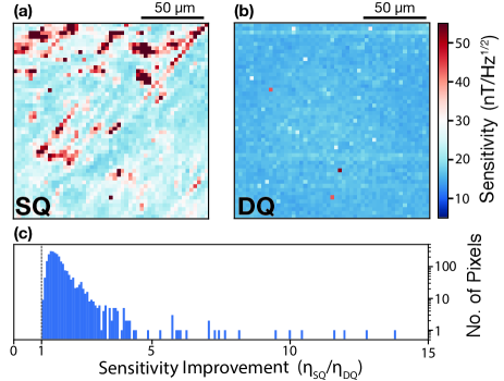
Figure 5: Imaging DC Magnetic Sensitivity. (a) Data acquired with SQ 2-Ramsey protocol when operating at an applied MW field $f_{\text{mw}}$ and free precession interval $\tau$ that optimize the median per-pixel magnetic sensitivity. (b) Data acquired with DQ 4-Ramsey protocol with optimal $f_{mw}^{\prime}$ and $\tau^{\prime}$, across the same field of view as (a). A few isolated, defective pixels with degraded sensitivity are visible. (c) Histogram of the improvement in relative sensitivity $\eta_{\text{SQ}}/\eta_{\text{DQ}}$ per pixel.

The resulting sensitivities $\eta_{\text{DQ}}$ and $\eta_{\text{SQ}}$ are plotted in Figs. 5(a) and 5(b). The median DQ 4-Ramsey per-pixel magnetic sensitivity $\eta_{\text{DQ}}\!=\,$15 (14, 16) nT Hz^-1/2 provides a factor of about 1.5$\times$ improvement compared to the SQ 2-Ramsey per-pixel magnetic sensitivity, $\eta_{\text{SQ}}\!=\,$22 (19, 34) nT Hz^-1/2 with voxel dimensions of ($2.5\times 2.4\times 1$) $\text{\,}{\mathrm{\SIUnitSymbolMicro m}}^{3}$. The upper and lower deciles, D₁₀ and D₉₀, are reported in parentheses. The typical uncertainty in the calculated per-pixel magnetic sensitivity, about 6 %, is dominated by the uncertainty in determining the parameters extracted from fitting the DC magnetometry curve in each pixel.

The median ($D_{10}$, $D_{90}$) volume-normalized sensitivities are therefore $\eta^{\text{V}}_{\text{DQ}}\!=\,$34 (32, 37) nT Hz${}^{-1/2}\,\upmu$m^3/2 and $\eta^{\text{V}}_{\text{SQ}}\!=\,$53 (44, 79) nT Hz${}^{-1/2}\,\upmu$m^3/2. We observe about a 4.7$\times$ reduction in the RIDR for $\eta_{\text{DQ}}$ ($\approx 14$%) compared to the RIDR of $\eta_{\text{SQ}}$ ($\approx 67$%). The improved median sensitivity and reduced spread across the field of view are attributed to the elimination of axial-stress-induced dephasing and resonance shifts for the DQ 4-Ramsey protocol, such that it is possible to operate at the optimal $\tau$ and applied MW frequencies $f_{\text{mw}}$ for an increased fraction of pixels simultaneously.

As illustrated in Fig. 5(c), all pixels exhibit improved magnetic sensitivity in the DQ sensing basis. Order-of-magnitude sensitivity improvements in the DQ basis are seen for the pixels corresponding to regions of diamond with higher stress gradients. In pixels with minimal stress-related effects, the improved magnetic sensitivity is attributed to (a) values of $f_{\text{mw}}$ and $\tau$ that are more optimal for an increased fraction of the pixels (see Appendix B) and (b) the effectively doubled gyromagnetic ratio in the DQ sensing basis. The latter enables faster measurements (increased maximum $F_{s}$ because $T_{2}^{*}\{\text{DQ}\}$, and thus the optimal free precession interval $\tau$, is reduced compared to $T_{2}^{*}\{\text{SQ}\}$) for the same phase accumulation (see Supplemental Material [24]). The residual $14$% spread in $\eta_{\text{DQ}}$ is a consequence of the Gaussian intensity profile of the excitation laser beam spot, which highlights the potential utility of optical beam-shaping techniques to enable further improvements.

The median volume-normalized magnetic sensitivity $\eta^{\text{V}}_{\text{DQ}}\!=\,$34 (32, 37) nT Hz${}^{-1/2}\,\upmu$m^3/2 demonstrated in this work coincidentally matches the value of $34\text{\,}\mathrm{nT}\text{\,}{\mathrm{\SIUnitSymbolMicro m}}^{3/2}\text{\,}{\mathrm{Hz}}^{-1/2}$ estimated in Ref. [33], which used photodiode-based CW-ODMR measurements to detect the single-neuron action potential from a living marine worm, M. infundibulum. Critically, the present work achieves a similar sensitivity while operating in an imaging modality, with degraded optical collection efficiency, and using NV${}^{\text{-}}$ centers along only a single crystal axis; whereas the non-imaging apparatus employed in Ref. [33] overlapped the resonances from two NV${}^{\text{-}}$ axes and had an approximately $16\times$ higher optical collection efficiency.

VI Outlook

The demonstrated magnetic imaging method using the DQ 4-Ramsey protocol enables uniform magnetic sensitivity across a field of view independent of inhomogeneity in the host diamond material and applied microwave control fields. In particular, the MW phase alternation scheme of the 4-Ramsey protocol [Fig. 2(c)] isolates the double quantum magnetic signal from residual single quantum signal, decoupling the measurement from common-mode resonance frequency shifts induced by axial stress and temperature drift. The achieved 100$\times$ reduction in sensitivity to common-mode shifts is broadly advantageous, not only for magnetic imaging but also for single-channel applications such as magnetic navigation [34].

These methods provide a path toward imaging a range of dynamic magnetic phenomena, including nanotesla-scale fields from single mammalian neurons or cardiomyocytes, as well as fields from integrated circuits and condensed matter systems. Increased optical excitation intensity and further diamond material development could yield additional improvements in volume-normalized magnetic sensitivity. Although pulsed magnetometry protocols favor operating near the NV${}^{\text{-}}$ center’s saturation intensity (1-3$\text{\,}\mathrm{mW}\text{\,}{\mathrm{\SIUnitSymbolMicro m}}^{-2}$ [35]) to minimize the initialization and readout durations [3], this work achieved optimal sensitivity when operating at an average intensity $\sim\!45\times$ below saturation. The lower intensity allowed the NV ensemble to maintain a favorable charge state fraction by reducing optical ionization of NV${}^{\text{-}}$ to NV${}^{\text{0}}$ [36, 37]. For this reason, future material development improving and stabilizing the NV charge fraction, for example by reducing the density of other parasitic defects that can act as charge acceptors [38], is critical.

The high-sensitivity, pulsed imaging method demonstrated here also enables applications beyond broadband magnetic microscopy such as parallelized, high-resolution NV${}^{\text{-}}$ ensemble NMR using AC magnetic field detection protocols. Additionally, the MW phase control utilized for the DQ 4-Ramsey protocol is sufficient to implement magnetically-insensitive measurement protocols [39, 40] as recently suggested by Ref. [41] for imaging the lattice damage induced by colliding weakly-interacting massive particles (WIMPs).

Author contributions statement

C.A.H., J.M.S., M.J.T., and E.B. conceived the experiments. C.A.H. and P.J.S. conducted the experiments. C.A.H. and J.M.S. analyzed the results. All authors contributed to and reviewed the manuscript. R.W. supervised the work.

Appendix A Experimental Details

An Agilent E9310A with built-in IQ modulation and a Windfreak SynthHD signal generator in combination with an external Marki-1545LMP IQ mixer provides the two-tone MW control fields and requisite phase control employed in this work. A Pulseblaster ESR-Pro with a 500 MHz clock controls the synchronization of applied MW pulses, optical pulses, and camera exposures (or photodiode readouts when applicable). Samarium cobalt ring-shaped magnets (as described in [16]) apply a $5\text{\,}\mathrm{mT}$ bias magnetic field used to split the $\ket{0}$ to $\ket{\pm 1}$ transitions.

Appendix B NV${}^{\text{-}}$ Ensemble Magnetometer Calibration

For the measurements in this work, the optimal free precession interval $\tau$ and applied MW frequency $f_{\text{mw}}$ are chosen to maximize the NV${}^{\text{-}}$ response $S$ to changes in magnetic-field $\frac{dS}{dB}$ (i.e., minimize the sensitivity $\eta$). Although the optimal $\tau$ is approximately equal to $T_{2}^{*}$ [3], the Ramsey fringe beating introduced by the hyperfine splitting of the NV${}^{\text{-}}$ restricts the possible choices of $\tau$ to discrete values. As a consequence, we select the nearest available $\tau$ to $T_{2}^{*}$ for each sensing basis. With the free precession interval $\tau$ fixed, the optimal $f_{\text{mw}}$ is determined by sweeping the applied MW frequency to emulate a change in magnetic field, producing a DC magnetometry curve from which $f_{\text{mw}}$ is chosen to maximize the slope $\frac{dS}{dB}$. To determine the optimal MW frequencies for DQ Ramsey measurements, $f_{\text{mw}}^{\prime}$, the two applied MW tones are swept differentially (one tone with positive detuning $+\delta$ and the second tone with an equal but opposite detuning $-\delta$). As with the SQ calibration, the values of $f_{\text{mw}}^{\prime}$ are chosen to maximize the NV${}^{\text{-}}$ response $\frac{dS}{dB}$. For all measurements using the heliCam, the free precession interval and MW frequency (or frequencies) are chosen to minimize the median per-pixel sensitivity across the field of view.

References

- Rondin et al. [2014] L. Rondin, J. P. Tetienne, T. Hingant, J. F. Roch, P. Maletinsky, and V. Jacques, Magnetometry with nitrogen-vacancy defects in diamond, Reports on Progress in Physics 77, 056503 (2014).
- Doherty et al. [2013] M. W. Doherty, N. B. Manson, P. Delaney, F. Jelezko, J. Wrachtrup, and L. C. L. Hollenberg, The nitrogen-vacancy colour centre in diamond, Physics Reports 528, 1 (2013).
- Barry et al. [2020] J. F. Barry, J. M. Schloss, E. Bauch, M. J. Turner, C. A. Hart, L. M. Pham, and R. L. Walsworth, Sensitivity optimization for nv-diamond magnetometry, Rev. Mod. Phys. 92, 015004 (2020).
- Levine et al. [2019] E. V. Levine, M. J. Turner, P. Kehayias, C. A. Hart, N. Langellier, R. Trubko, D. R. Glenn, R. R. Fu, and R. L. Walsworth, Principles and techniques of the quantum diamond microscope, Nanophotonics 8, 1945 (2019).
- Glenn et al. [2017] D. R. Glenn, R. R. Fu, P. Kehayias, D. Le Sage, E. A. Lima, B. P. Weiss, and R. L. Walsworth, Micrometer‐scale magnetic imaging of geological samples using a quantum diamond microscope, Geochemistry, Geophysics, Geosystems 18, 3254 (2017).
- Simpson et al. [2016] D. A. Simpson, J.-P. Tetienne, J. M. McCoey, K. Ganesan, L. T. Hall, S. Petrou, R. E. Scholten, and L. C. L. Hollenberg, Magneto-optical imaging of thin magnetic films using spins in diamond, Scientific Reports 6, 22797 (2016).
- McCoey et al. [2020] J. M. McCoey, M. Matsuoka, R. W. de Gille, L. T. Hall, J. A. Shaw, J. Tetienne, D. Kisailus, L. C. L. Hollenberg, and D. A. Simpson, Quantum Magnetic Imaging of Iron Biomineralization in Teeth of the Chiton <i>Acanthopleura hirtosa</i>, Small Methods 4, 1900754 (2020).
- Tetienne et al. [2017] J.-P. Tetienne, N. Dontschuk, D. A. Broadway, A. Stacey, D. A. Simpson, and L. C. L. Hollenberg, Quantum imaging of current flow in graphene, Science Advances 3, e1602429 (2017).
- Ku et al. [2020] M. J. H. Ku, T. X. Zhou, Q. Li, Y. J. Shin, J. K. Shi, C. Burch, L. E. Anderson, A. T. Pierce, Y. Xie, A. Hamo, U. Vool, H. Zhang, F. Casola, T. Taniguchi, K. Watanabe, M. M. Fogler, P. Kim, A. Yacoby, and R. L. Walsworth, Imaging viscous flow of the Dirac fluid in graphene, Nature 583, 537 (2020).
- Turner et al. [2020] M. J. Turner, N. Langellier, R. Bainbridge, D. Walters, S. Meesala, T. M. Babinec, P. Kehayias, A. Yacoby, E. Hu, M. Lončar, R. L. Walsworth, and E. V. Levine, Magnetic Field Fingerprinting of Integrated-Circuit Activity with a Quantum Diamond Microscope, Physical Review Applied 14, 014097 (2020).
- Le Sage et al. [2013] D. Le Sage, K. Arai, D. R. Glenn, S. J. DeVience, L. M. Pham, L. Rahn-Lee, M. D. Lukin, A. Yacoby, A. Komeili, and R. Walsworth, Optical magnetic imaging of living cells., Nature 496, 486 (2013).
- Glenn et al. [2015] D. R. Glenn, K. Lee, H. Park, R. Weissleder, A. Yacoby, M. D. Lukin, H. Lee, R. L. Walsworth, and C. B. Connolly, Single-cell magnetic imaging using a quantum diamond microscope, Nature Methods 12, 736 (2015).
- Kehayias et al. [2019] P. Kehayias, M. J. Turner, R. Trubko, J. M. Schloss, C. A. Hart, M. Wesson, D. R. Glenn, and R. L. Walsworth, Imaging crystal stress in diamond using ensembles of nitrogen-vacancy centers, Phys. Rev. B 100, 174103 (2019).
- Kazi et al. [2021] Z. Kazi, I. M. Shelby, H. Watanabe, K. M. Itoh, V. Shutthanandan, P. A. Wiggins, and K.-M. C. Fu, Wide-field dynamic magnetic microscopy using double-double quantum driving of a diamond defect ensemble (2021), arXiv:2002.06237 .
- Fescenko et al. [2020] I. Fescenko, A. Jarmola, I. Savukov, P. Kehayias, J. Smits, J. Damron, N. Ristoff, N. Mosavian, and V. M. Acosta, Diamond magnetometer enhanced by ferrite flux concentrators, Phys. Rev. Research 2, 023394 (2020).
- Bauch et al. [2018] E. Bauch, C. A. Hart, J. M. Schloss, M. J. Turner, J. F. Barry, P. Kehayias, S. Singh, and R. L. Walsworth, Ultralong dephasing times in solid-state spin ensembles via quantum control, Phys. Rev. X 8, 031025 (2018).
- Mamin et al. [2014] H. J. Mamin, M. H. Sherwood, M. Kim, C. T. Rettner, K. Ohno, D. D. Awschalom, and D. Rugar, Multipulse double-quantum magnetometry with near-surface nitrogen-vacancy centers, Physical Review Letters 113, 030803 (2014).
- Fang et al. [2013] K. Fang, V. M. Acosta, C. Santori, Z. Huang, K. M. Itoh, H. Watanabe, S. Shikata, and R. G. Beausoleil, High-sensitivity magnetometry based on quantum beats in diamond nitrogen-vacancy centers, Physical Review Letters 110, 130802 (2013).
- Jamonneau et al. [2016] P. Jamonneau, M. Lesik, J. P. Tetienne, I. Alvizu, L. Mayer, A. Dréau, S. Kosen, J.-F. Roch, S. Pezzagna, J. Meijer, T. Teraji, Y. Kubo, P. Bertet, J. R. Maze, and V. Jacques, Competition between electric field and magnetic field noise in the decoherence of a single spin in diamond, Physical Review B 93, 024305 (2016).
- Barson et al. [2017] M. S. J. Barson, P. Peddibhotla, P. Ovartchaiyapong, K. Ganesan, R. L. Taylor, M. Gebert, Z. Mielens, B. Koslowski, D. A. Simpson, L. P. McGuinness, J. McCallum, S. Prawer, S. Onoda, T. Ohshima, A. C. Bleszynski Jayich, F. Jelezko, N. B. Manson, and M. W. Doherty, Nanomechanical sensing using spins in diamond, Nano Letters 17, 1496 (2017).
- Udvarhelyi et al. [2018] P. Udvarhelyi, V. O. Shkolnikov, A. Gali, G. Burkard, and A. Pályi, Spin-strain interaction in nitrogen-vacancy centers in diamond, Phys. Rev. B 98, 075201 (2018).
- Barfuss et al. [2019] A. Barfuss, M. Kasperczyk, J. Kölbl, and P. Maletinsky, Spin-stress and spin-strain coupling in diamond-based hybrid spin oscillator systems, Phys. Rev. B 99, 174102 (2019).
- Dolde et al. [2011] F. Dolde, H. Fedder, M. W. Doherty, T. Nöbauer, F. Rempp, G. Balasubramanian, T. Wolf, F. Reinhard, L. C. L. Hollenberg, F. Jelezko, and J. Wrachtrup, Electric-field sensing using single diamond spins, Nature Physics 7, 459 (2011).
- [24] See the Supplemental Material at [URL to be inserted] for additional information on the NV Hamiltonian, DQ 4-Ramsey measurement protocol, and magnetic imaging results.
- Friel et al. [2009] I. Friel, S. L. Clewes, H. K. Dhillon, N. Perkins, D. J. Twitchen, and G. A. Scarsbrook, Control of surface and bulk crystalline quality in single crystal diamond grown by chemical vapour deposition, Diamond and Related Materials 18, 808 (2009).
- Bar-Gill et al. [2013] N. Bar-Gill, L. M. Pham, A. Jarmola, D. Budker, and R. L. Walsworth, Solid-state electronic spin coherence time approaching one second., Nature Communications 4, 1743 (2013).
- Przybylski et al. [2017] A. Przybylski, B. Thiel, J. Keller-Findeisen, B. Stock, and M. Bates, Gpufit: An open-source toolkit for GPU-accelerated curve fitting, Scientific Reports 7, 15722 (2017).
- Taylor et al. [2008] J. M. Taylor, P. Cappellaro, L. Childress, L. Jiang, D. Budker, P. R. Hemmer, A. Yacoby, R. Walsworth, and M. D. Lukin, High-sensitivity diamond magnetometer with nanoscale resolution, Nature Physics 4, 810 (2008).
- Le Sage et al. [2012] D. Le Sage, L. M. Pham, N. Bar-Gill, C. Belthangady, M. D. Lukin, A. Yacoby, and R. L. Walsworth, Efficient photon detection from color centers in a diamond optical waveguide, Physical Review B 85, 121202(R) (2012).
- Bal et al. [2012] M. Bal, C. Deng, J. L. Orgiazzi, F. R. Ong, and A. Lupascu, Ultrasensitive magnetic field detection using a single artificial atom, Nature Communications 3, 1324 (2012).
- Schoenfeld and Harneit [2011] R. S. Schoenfeld and W. Harneit, Real time magnetic field sensing and imaging using a single spin in diamond, Physical Review Letters 106, 030802 (2011).
- Schloss et al. [2018] J. M. Schloss, J. F. Barry, M. J. Turner, and R. L. Walsworth, Simultaneous Broadband Vector Magnetometry Using Solid-State Spins, Physical Review Applied 10, 034044 (2018).
- Barry et al. [2016] J. F. Barry, M. J. Turner, J. M. Schloss, D. R. Glenn, Y. Song, M. D. Lukin, H. Park, and R. L. Walsworth, Optical magnetic detection of single-neuron action potentials using quantum defects in diamond, Proceedings of the National Academy of Sciences of the United States of America 113, 14133 (2016).
- Canciani and Raquet [2016] A. Canciani and J. Raquet, Absolute Positioning Using the Earth’s Magnetic Anomaly Field, Navigation, Journal of the Institute of Navigation 63, 111 (2016).
- Wee et al. [2007] T.-L. Wee, Y.-K. Tzeng, C.-C. Han, H.-C. Chang, W. Fann, J.-H. Hsu, K.-M. Chen, and Y.-C. Yu, Two-photon excited fluorescence of nitrogen-vacancy centers in proton-irradiated type Ib diamond, Journal of Physical Chemistry A 111, 9379 (2007).
- Alsid et al. [2019] S. T. Alsid, J. F. Barry, L. M. Pham, J. M. Schloss, M. F. O’Keeffe, P. Cappellaro, and D. A. Braje, Photoluminescence Decomposition Analysis: A Technique to Characterize N - V Creation in Diamond, Physical Review Applied 12, 044003 (2019).
- Aude Craik et al. [2020] D. Aude Craik, P. Kehayias, A. Greenspon, X. Zhang, M. Turner, J. Schloss, E. Bauch, C. Hart, E. Hu, and R. Walsworth, Microwave-Assisted Spectroscopy Technique for Studying Charge State in Nitrogen-Vacancy Ensembles in Diamond, Physical Review Applied 14, 014009 (2020).
- Edmonds et al. [2021] A. M. Edmonds, C. A. Hart, M. J. Turner, P.-O. Colard, J. M. Schloss, K. Olsson, R. Trubko, M. L. Markham, A. Rathmill, B. Horne-Smith, W. Lew, A. Manickam, S. Bruce, P. G. Kaup, J. C. Russo, M. J. DiMario, J. T. South, J. T. Hansen, D. J. Twitchen, and R. Walsworth, Characterisation of CVD diamond with high concentrations of nitrogen for magnetic-field sensing applications, Materials for Quantum Technology 10.1088/2633-4356/abd88a (2021).
- Toyli et al. [2013] D. M. Toyli, C. F. de las Casas, D. J. Christle, V. V. Dobrovitski, and D. D. Awschalom, Fluorescence thermometry enhanced by the quantum coherence of single spins in diamond, Proceedings of the National Academy of Sciences 110, 8417 (2013).
- Hodges et al. [2013] J. S. Hodges, N. Y. Yao, D. Maclaurin, C. Rastogi, M. D. Lukin, and D. Englund, Timekeeping with electron spin states in diamond, Physical Review A 87, 032118 (2013).
- Rajendran et al. [2017] S. Rajendran, N. Zobrist, A. O. Sushkov, R. Walsworth, and M. Lukin, A method for directional detection of dark matter using spectroscopy of crystal defects, Physical Review D 96, 035009 (2017).