Multiflypes of rectangular diagrams of links

Abstract.

We introduce a new very large family of transformations of rectangular diagrams of links that preserve the isotopy class of the link. We provide an example when two diagrams of the same complexity are related by such a transformation and are not obtained from one another by any sequence of ‘simpler’ moves not increasing the complexity of the diagram along the way.

Introduction

It is shown in [3] that rectangular diagrams of links (also known as arc-presentations and grid diagrams) allow one to solve certain decidability problems in knot theory using one of the most naive approaches, which is based on monotonic simplification. Namely, one can decide wether the given rectangular diagram represents an unknot, a split link, or a composite link by successively applying all possible sequences of elementary moves not increasing the number of edges, and check if any of the obtained diagrams is trivial, split, or composite, respectively. Previously known solutions of these problems, the first of which are due to W. Haken [7] and H. Schubert [11], use much more advanced technique.

Elementary moves involved in the monotonic simplification procedure mentioned above include only very simple transformations called exchange moves, stabilizations and destabilizations. There are several reasons to look for more general families of moves preserving the isotopy class of the link.

One reason is that more general moves might make the monotonic simplification faster. To this writing, the algorithms based on monotonic simplification of rectangular diagrams have exponential asymptotic complexity due to the fact that the simplification is not strictly monotonic.

Another reason is a hope that more general moves would allow to solve more algorithmic problems in the same manner. One of such problems, which is most natural to consider after the unknotedness, splitness, and factorization ones, is finding the JSJ-decomposition of the link complement (solved in [5, 6] with the help of Kneser–Haken normal surfaces). It is also natural to try extending the monotonic simplification approach to general links.

Finally, studying the combinatorics of more general transformations may result in new classification results and more efficient estimates for the number of elementary moves (or Reidemeister moves for planar diagrams) needed to transform one diagram to another if they represent isotopic links.

A class of transformations of rectangular diagrams generalizing elementary moves was introduced in [2], where the new transformations were called flypes, since in certain situations they converted into flypes of the respective planar diagrams. However, these moves did not help to advance in any of the directions listed above.

In particular, it is shown in [8] that flypes of rectangular diagrams do not allow to detect satellite knots by means of monotonic simplification. An example of two rectangular diagrams, which we denote here by $R_{\text{{\char 16\relax}}}$ and $R_{\text{{\char 27\relax}}}$ (with the former modified in an obvious way by exchange moves), representing the same satellite knot are provided (see [8, Section 7]) such that $R_{\text{{\char 27\relax}}}$ is not ‘obviously satellite’ and admits no complexity preserving flype changing the combinatorial type of the diagram, whereas $R_{\text{{\char 16\relax}}}$ is ‘obviously satellite’.

Below we introduce a much more general type of moves, which we call multiflypes because they have been originally thought of as several flypes performed simultaneously. The main result of the present paper is a proof that these new moves preserve the isotopy class of the link. We also use the example from [8] to show an advantage of the new moves: they allow to proceed from $R_{\text{{\char 27\relax}}}$ to $R_{\text{{\char 16\relax}}}$ without increasing the complexity along the way.

1. Preliminaries

We denote by $\mathbb{T}^{2}$ the two-dimensional torus $\mathbb{S}^{1}\times\mathbb{S}^{1}$, and by $\theta,\varphi$ the angular coordinates on $\mathbb{T}^{2}$, which run through $\mathbb{S}^{1}=\mathbb{R}/(2\pi\mathbb{Z})$. Denote by $p_{\theta}$ and $p_{\varphi}$ the projection maps from $\mathbb{T}^{2}$ to the first and the second $\mathbb{S}^{1}$-factors, respectively. For any $\theta_{0},\varphi_{0}\in\mathbb{S}^{1}$, we put $m_{\theta_{0}}=\{\theta_{0}\}\times\mathbb{S}^{1}$, $\ell_{\varphi_{0}}=\mathbb{S}^{1}\times\{\varphi_{0}\}$, and call these a meridian and a longitude of $\mathbb{T}^{2}$, respectively.

For two distinct points $x_{1},x_{2}\in\mathbb{S}^{1}$ we denote by $[x_{1};x_{2}]$ (respectively, $(x_{1};x_{2})$) the closed (respectively, open) interval in $\mathbb{S}^{1}$ starting at $x_{1}$ and ending at $x_{2}$.

Definition 1.1.

An oriented rectangular diagram of a link is a non-empty finite subset $R\subset\mathbb{T}^{2}$ with a decomposition $R=R^{+}\sqcup R^{-}$ into a disjoint union of two subsets $R^{+}$ and $R^{-}$ such that we have $p_{\theta}(R^{+})=p_{\theta}(R^{-})$, $p_{\varphi}(R^{+})=p_{\varphi}(R^{-})$, and each of $p_{\theta}$, $p_{\varphi}$ restricted to each of $R^{+}$, $R^{-}$ is injective.

The elements of $R$ (respectively, of $R^{+}$ or $R^{-}$) are called vertices (respectively, positive vertices or negative vertices) of $R$.

Pairs $(u,v)$ of vertices of $R$ such that $p_{\theta}(u)=p_{\theta}(v)$ (respectively, $p_{\varphi}(u)=p_{\varphi}(v)$) are called vertical (respectively, horizontal) edges of $R$.

All points in

$$\bigl{(}p_{\theta}(R)\times p_{\varphi}(R)\bigr{)}\setminus R\subset\mathbb{T}^{2}$$

are called crossings of $R$.

With every oriented rectangular diagram of a link $R$ one associates a topological oriented link type $\mathscr{L}(R)$ as follows. First, choose a meridian $m_{\theta_{0}}$ and a longitude $\ell_{\varphi_{0}}$ not passing through a vertex of $R$ and cut $\mathbb{T}^{2}$ along $m_{\theta_{0}}\cup\ell_{\varphi_{0}}$ to obtain a square. Then connect, by a straight line segment, every pair of vertices of $R$ forming an edge of $R$. At every intersection point, regard the vertical arc as overcrossing. The vertical arcs are oriented from a positive vertex to a negative one, and horizontal arcs from a negative vertex to a positive one. The obtained oriented planar diagram of a link represents $\mathscr{L}(R)$. An example is shown in Figure 1.1.

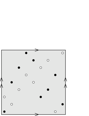
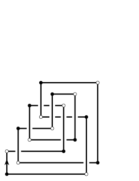
$R$		a representative of $\mathscr{L}(R)$

Figure 1.1. A rectangular diagram of a link and a planar diagram of the corresponding link

Here and below positive vertices are shown in black, and negative vertices in white.

It will be convenient in the sequel to represent any rectangular diagram of a link $R$ by the following function $\sigma:\mathbb{T}^{2}\rightarrow\{-1,0,1\}$, which will be called the characteristic function of $R$:

$$\sigma_{R}(v)=\left\{\begin{aligned} 0,&\text{ if }v\notin R,\\ 1,&\text{ if }v\in R^{+},\\ -1,&\text{ if }v\in R^{-}.\end{aligned}\right.$$

By a rectangle we mean a subset $r$ of $\mathbb{T}^{2}$ of the form $[\theta_{1};\theta_{2}]\times[\varphi_{1};\varphi_{2}]$, where $\theta_{1},\theta_{2},\varphi_{1},\varphi_{2}\in\mathbb{S}^{1}$. With every rectangle $r=[\theta_{1};\theta_{2}]\times[\varphi_{1};\varphi_{2}]$ we associate a trivial rectangular diagram of a link $R(r)$ as follows:

$$R(r)^{+}=\{(\theta_{1},\varphi_{1}),(\theta_{2},\varphi_{2})\},\quad R(r)^{-}=\{(\theta_{1},\varphi_{2}),(\theta_{2},\varphi_{1})\}.$$

Clearly, $R(r)$ represents an unknot.

For any rectangle $r$, we denote $\sigma_{R(r)}$ by $\sigma_{r}$ for brevity.

Definition 1.2.

Let $R$ and $R^{\prime}$ be oriented rectangular diagrams of links. The passages from $R$ to $R^{\prime}$ and from $R^{\prime}$ to $R$ are called elementary moves if there is a rectangle $r$ such that:

1. $\sigma_{R}-\sigma_{R^{\prime}}=\sigma_{r}$

2. the intersection $R\cap r$ consists of exactly one, two, or three successive vertices of $r$.

Elementary moves defined in this way include all versions of exchange moves (also called commutations in the literature), stabilizations and destabilizations introduced in earlier works [1, 3], and also some compositions of these moves with several exchange moves. It is easy to verify that all elementary moves preserve the isotopy class of the link associated with the diagram.

2. Definition of a multiflype and the main result

There are four similar versions of multiflypes related with one another by symmetries $(\theta,\varphi)\mapsto(-\theta,\varphi)$ and $(\theta,\varphi)\mapsto(\theta,-\varphi)$. Each type of multiflypes is assigned an arrow $\nearrow$, $\nwarrow$, $\swarrow$, or $\searrow$, on which the symmetries act accordingly.

Let $R$ be an oriented rectangular diagram of a link, and let $A\subset\mathbb{T}^{2}$ be an annulus such that:

1. the boundary $\partial A$ is transverse to all meridians and longitudes, and the slope of $\partial A$ is positive, that is, $d\varphi/d\theta>0$ on $\partial A$;

2. $\partial A$ misses all crossings of $R$ (which are defined in Definition 1.1);

3. there is no pair of distinct points $u,v\in\partial A$ not forming a vertical (respectively, horizontal) edge of $R$ but lying on the same meridian (respectively, longitude) and such that $p_{\varphi}(u),p_{\varphi}(v)\in p_{\varphi}(R)$ (respectively, $p_{\theta}(u),p_{\theta}(v)\in p_{\theta}(R)$).

We denote by $\partial_{1}A$ the connected component of $\partial A$ defined by demanding that a small push off of $\partial_{1}A$ in the $(1,-1)$-direction lies outside of $A$. The other connected component is denoted by $\partial_{2}A$.

For every point $v\in A\setminus\partial A$, denote by $r_{v}$ a rectangle $[\theta_{1};\theta_{2}]\times[\varphi_{1};\varphi_{2}]$ such that $(\theta_{1},\varphi_{1})=v$, $(\theta_{2},\varphi_{1})\in\partial_{1}A$, and $(\theta_{1},\varphi_{2})\in\partial_{2}A$ (see Figure 2.1).

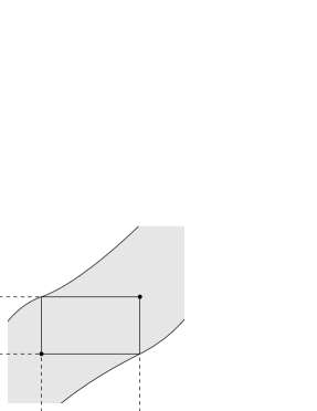
Figure 2.1. The rectangle $r_{v}$

Such a rectangle is clearly unique. Denote by $\overline{v}$ the vertex of $r_{v}$ opposite to $v$.

Proposition 2.1.

There exists a (unique) oriented rectangular diagram of a link $R^{\prime}$ such that

(2.1) $$\sigma_{R^{\prime}}=\sigma_{R}-\sum_{v\in R\cap(A\setminus\partial A)}\sigma_{R}(v)\sigma_{r_{v}}.$$

Proof.

We give a geometric interpretation of (2.1) from which it is clear that $R^{\prime}$ is a well defined oriented rectangular diagram of a link.

First, note that, on any meridian $m_{\theta_{0}}$ and on any longitude $\ell_{\varphi_{0}}$, the right hand side of (2.1) sum up to zero, since so does each summand in it. So, it suffices to verify that the right hand side of (2.1) takes only values in $\{-1,0,1\}$, and on every meridian and longitude, it takes non-zero values at at most two points.

The map $v\mapsto\overline{v}$ is clearly a bijection from $A\setminus\partial A$ to itself. If $v\in R\cap(A\setminus\partial A)$, then the subtraction of $\sigma_{R}(v)\sigma_{r_{v}}$ from $\sigma_{R}$, geometrically, results in removing $v$ from the diagram and adding $\overline{v}$ with the opposite sign. So, inside the domain $A\setminus\partial A$, the geometric meaning of (2.1) is the replacement of every vertex $v$ in $R\cap(A\setminus\partial A)$ by the respective vertex $\overline{v}$ having the opposite sign.

Some vertices are also removed or added at $\partial A$, and the rule defined by (2.1) is as follows. Let $(\theta_{0},\varphi_{0})\in\partial_{1}A$, and let $[\theta_{1};\theta_{0}]\times\{\varphi_{0}\}$ be a maximal horizontal arc contained in $A$. If there are two or no vertices of $R$ in the open arc $(\theta_{1};\theta_{0})\times\{\varphi_{0}\}$, then no change of the diagram occurs at $(\theta_{0},\varphi_{0})$. If this arc contains exactly one vertex and $(\theta_{0},\varphi_{0})$ is also a vertex of $R$, then this vertex is removed. Otherwise, a vertex is added at $(\theta_{0},\varphi_{0})$.

The change of the diagram at any $(\theta_{0},\varphi_{0})\in\partial_{2}A$ depends similarly on the number of vertices of $R$ in $\{\theta_{0}\}\times(\varphi_{1};\varphi_{0})$, where $\{\theta_{0}\}\times[\varphi_{1};\varphi_{0}]$ is a maximal vertical arc contained in $A$.

Thus, the only way in which the right hand side of (2.1) may fail to be the characteristic function of an oriented rectangular diagram is that it takes non-zero values at four or more points contained in a single meridian or longitude. One can see that the conditions imposed on the choice of $A$ guarantee that this does not happen. ∎

The passage from $R$ to $R^{\prime}$ defined by (2.1) is called a $\nearrow$-multiflype (based on $A$). The other types of multiflypes are defined as follows:

$s_{\updownline}(R)\mapsto s_{\updownline}(R^{\prime})$ is a $\nwarrow$-multiflype, $s_{\leftrightline}(R)\mapsto s_{\leftrightline}(R^{\prime})$ is a $\searrow$-multiflype, $(s_{\updownline}\circ s_{\leftrightline})(R)\mapsto(s_{\updownline}\circ s_{\leftrightline})(R^{\prime})$ is a $\swarrow$-multiflype,

where

$$s_{\updownline}(\theta,\varphi)=(-\theta,\varphi),\quad s_{\leftrightline}(\theta,\varphi)=(\theta,-\varphi).$$

The proof of the following two statements is easy and left to the reader.

Proposition 2.2.

The inverse of a $\nearrow$-multiflype (respectively, $\nwarrow$-multiflype) is a $\swarrow$-multiflype (respectively, $\searrow$-multiflype).

Proposition 2.3.

Elementary moves of oriented rectangular diagrams of links are exactly multiflypes such that the interior of the respective annulus $A$ contains exactly one vertex of the diagram.

The following theorem is the main result of this paper.

Theorem 2.1.

If $R\mapsto R^{\prime}$ is a multiflype, then $\mathscr{L}(R)=\mathscr{L}(R^{\prime})$.

The proof will be given in Section 4.

3. An example

Shown at the top of Figure 3.1 is an oriented rectangular diagram $R_{\text{{\char 16\relax}}}$ of a link which is a satellite knot. Namely, it is a 2-cable of the trefoil knot, and the satellite structure is clearly visible from the diagram.

The diagram $R_{\text{{\char 27\relax}}}$ in the middle row represents the same knot, but it is already non-trivial to detect the satellite structure from this diagram. It is easy to see that no combinatorially non-trivial and complexity-preserving elementary move can be applied to $R_{\text{{\char 27\relax}}}$. Moreover, it is shown in [8] that the combinatorial structure of $R_{\text{{\char 27\relax}}}$ cannot be changed by more general moves called flypes in [2], without introducing more edges. Thus, with only flypes at hand, the monotonic simplification method does fails at detecting the satellite structure of this knot from the diagram $R_{\text{{\char 27\relax}}}$.

This detection becomes possible with the help of multiflypes. The diagram $R_{\text{{\char 30\relax}}}$ in Figure 3.1, if viewed combinatorially, is obtained from $R_{\text{{\char 27\relax}}}$ by a single multiflype preserving the number of edges. This is demonstrated in the bottom row of Figure 3.1, where the respective annulus $A$ is shown as a shaded region, and all involved rectangles of the form $r_{v}$ are also indicated.

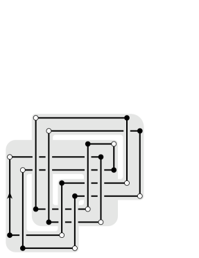
$$R_{\text{{\char 16\relax}}}$$

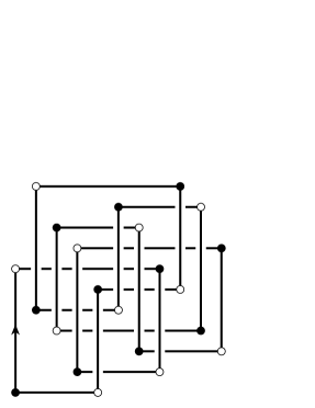
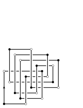
$R_{\text{{\char 27\relax}}}$		$R_{\text{{\char 30\relax}}}$

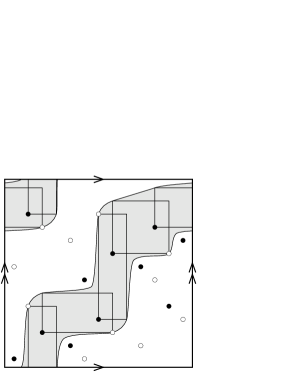
Figure 3.1. The transitions $R_{\text{{\char 27\relax}}}\mapsto R_{\text{{\char 30\relax}}}$ and $R_{\text{{\char 30\relax}}}\mapsto R_{\text{{\char 27\relax}}}$ are (combinatorially) a $\swarrow$-flype and a $\nearrow$-flype, respectively

It is then two elementary moves preserving the number of edges (exchange moves) to obtain $R_{\text{{\char 16\relax}}}$ from $R_{\text{{\char 30\relax}}}$ (a shift one step up is also in order).

4. Proof of Theorem 2.1

4.1. Preparations

We keep the notation and the settings from Section 2. In particular, we use the bijection $v\mapsto\overline{v}$ from $A\setminus\partial A$ to itself and extend it to the whole of $A$ by continuity. Namely, for $v\in\partial_{1}A$ (respectively, $v\in\partial_{2}A$), the point $\overline{v}$ is defined by the condition that a connected component of the intersection of some meridian (respectively, longitude) with $A$ has the form $\{\theta_{0}\}\times[\varphi_{1};\varphi_{2}]$ with $(\theta_{0},\varphi_{1})=v$ and $(\theta_{0},\varphi_{2})=\overline{v}$ (respectively, $[\theta_{1};\theta_{2}]\times\{\varphi_{0}\}$ with $(\theta_{1},\varphi_{0})=v$ and $(\theta_{2},\varphi_{0})=\overline{v}$). If $v\in\partial A$, then the notation $\sigma_{r_{v}}$ refers to the identically zero function on $\mathbb{T}^{2}$.

We assume that $R\mapsto R^{\prime}$ is a $\nearrow$-multiflype based an annulus $A\subset\mathbb{T}^{2}$.

We say that an elementary move $R_{1}\mapsto R_{2}$ is performed inside $A$ if $\sigma_{R_{1}}-\sigma_{R_{2}}=\pm\sigma_{r}$, where $r$ is a rectangle contained in $A$ such that $r\cap R_{1}\subset V(r)$, where by $V(r)$ we denote the set of vertices of $r$.

Lemma 4.1.

Let $R\mapsto R_{1}$ be an elementary move performed inside $A$. Suppose that $A$ is still suitable for defining a $\nearrow$-multiflype on $R_{1}$. Let $R_{1}\mapsto R_{1}^{\prime}$ be this $\nearrow$-multiflype. Then $R_{1}\mapsto R_{1}^{\prime}$ is an elementary move performed inside $A$.

Proof.

Let $r\subset A$ be a rectangle such that $\sigma_{R}-\sigma_{R_{1}}=\epsilon\sigma_{r}$ and $r\cap R\subset V(r)$, where $\epsilon=\pm 1$, and let $v_{1},v_{2},v_{3},v_{4}$ be the vertices of $r$ numbered counterclockwise with $v_{1}$ being the bottom left vertex.

Equality (2.1) can be rewritten as

$$\sigma_{R^{\prime}}=\sigma_{R}-\sum_{v\in A}\sigma_{R}(v)\sigma_{r_{v}},$$

since there are only finitely many points at which $\sigma_{R}$ does not vanish, and for $v\in\partial A$ we put $\sigma_{r_{v}}\equiv 0$. Similarly, we have

$$\sigma_{R_{1}^{\prime}}=\sigma_{R_{1}}-\sum_{v\in A}\sigma_{R_{1}}(v)\sigma_{r_{v}},$$

and hence,

$$\sigma_{R^{\prime}}-\sigma_{R^{\prime}_{1}}=\epsilon\Bigl{(}\sigma_{r}-\sum_{v\in A}\sigma_{r}(v)\sigma_{r_{v}}\Bigr{)}=\epsilon\Bigl{(}\sigma_{r}-\sum_{v\in V(r)}\sigma_{r}(v)\sigma_{r_{v}}\Bigr{)}.$$

One can verify (consult Figure 4.1) that, whichever rectangle $r\subset A$ is,

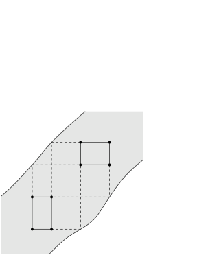
Figure 4.1. The rectangle $\overline{r}$

the following identity holds

$$\sigma_{r}-\sum_{v\in V(r)}\sigma_{r}(v)\sigma_{r_{v}}=-\sigma_{\overline{r}},$$

where $\overline{r}=\{\overline{u}:u\in r\}$ is also a rectangle, and the vertices of $\overline{r}$ listed clockwise are $\overline{v}_{1}$, $\overline{v}_{2}$, $\overline{v}_{3}$, $\overline{v}_{4}$. Thus, we have

$$\sigma_{R_{1}^{\prime}}=\sigma_{R_{1}}+\epsilon\sigma_{\overline{r}}.$$

We have seen in the proof of Proposition 2.1 the following:

$$R^{\prime}\cap(A\setminus\partial A)=\{\overline{v}:v\in R\cap(A\setminus\partial A)\}.$$

Since $r\setminus V(r)\subset A\setminus\partial A$ and $r\cap R\subset V(r)$, we have $\overline{r}\cap R^{\prime}\subset V(\overline{r})$.

To ensure that $R^{\prime}\mapsto R_{1}^{\prime}$ is an elementary move it remains to verify that $R^{\prime}\cap V(\overline{r})$ consists of exactly one, two, or three successive vertices of $\overline{r}$. This is equivalent to saying that there are two vertices of $\overline{r}$ opposite to one another and such that exactly one of them belongs to $R^{\prime}$.

If $r\subset A\setminus\partial A$ then $\overline{v}_{i}\in R^{\prime}$ if and only if $v_{i}\in R$. In this case, $R^{\prime}\cap V(\overline{r})$ consists of exactly one, two, or three successive vertices of $\overline{r}$, since the same is true for $R\cap V(r)$ and $r$ by assumption.

The vertices $v_{1}$ and $v_{3}$ always lie in $A\setminus\partial A$, hence, if $R\cap\{v_{1},v_{3}\}=\{v_{1}\}\text{ or }\{v_{3}\}$, then $R^{\prime}\cap\{\overline{v}_{1},\overline{v}_{3}\}=\{\overline{v}_{1}\}\text{ or }\{\overline{v}_{3}\}$, so, the required condition on the intersection $R^{\prime}\cap V(\overline{r})$ holds true.

We are left with the cases when $R\cap\{v_{1},v_{3}\}=\varnothing\text{ or }\{v_{1},v_{3}\}$, and $r\cap\partial A\neq\varnothing$. We may assume without loss of generality that $R\cap r=\{v_{1},v_{2},v_{3}\}$, since the other remaining cases are obtained from this one by exchanging $R$ with $R_{1}$ and/or $\theta$ with $\varphi$.

In this case, $v_{4}$ is a crossing of $R$, therefore, by assumption, $v_{4}\notin\partial A$. The only non-trivial option for $r\cap\partial A$ is $\{v_{2}\}$. It is a direct check that, in this case, $R^{\prime}\cap V(\overline{r})=\{\overline{v}_{1},\overline{v}_{2},\overline{v}_{3}\}$. This completes the proof of the lemma.∎

For any point $v\in A\setminus\partial A$, denote by $r^{v}$ the rectangle $r_{u}$ with $\overline{u}=v$. Denote also by $\Delta^{+}_{v}$ (respectively, $\Delta^{-}_{v}$) the closure of the connected component of $A\setminus(r_{v}\cup r^{v})$ having empty intersection with $\partial_{1}A$ (respectively, $\partial_{2}A$), and by $\Omega_{v}$ the union $\Delta^{+}_{v}\cup\Delta^{-}_{v}\cup r_{v}$ (see Figure 4.2).

Figure 4.2. The domain $\Omega_{v}$

By $\partial_{*}\Omega_{v}$ we denote the following part of the boundary of $\Omega_{v}$:

$$\partial_{*}\Omega_{v}=(\partial\Omega_{v}\setminus\partial A)\cap r^{v}.$$

One can see that $u\in\partial_{*}\Omega_{v}$ is equivalent to $\overline{u}\in\partial_{*}\Omega_{\overline{v}}$, and $\partial_{*}\Omega_{\overline{v}}\subset\partial\Omega_{v}$.

Now choose a point $u_{0}\in A\setminus\partial A$ such that neither $u_{0}$ nor $\overline{u}_{0}$ belongs to a meridian or a longitude containing an edge of $R$. Denote $\overline{u}_{0}$ by $u_{1}$.

The proof of Theorem 2.1 is by induction in the number of vertices of $R$ contained in $\Omega_{u_{0}}\setminus\partial A$.

4.2. The induction base

Suppose that $R\cap(\Omega_{u_{0}}\setminus\partial A)=\varnothing$. Pick a smooth parametrized path $t\mapsto u_{t}$, $t\in[0;1]$, starting at $u_{0}$ and ending at $u_{1}$ and such that:

1. $u_{t}\in A\setminus(\partial A\cup\Omega_{u_{0}})$ for all $t\in(0;1)$;

2. $u_{t}$ avoids crossings and vertices of $R$;

3. $d\theta(u_{t})/dt<0$ and $d\varphi(u_{t})/dt<0$ for all $t\in[0;1]$.

Observe that we also have $d\theta(\overline{u}_{t})/dt<0$ and $d\varphi(\overline{u}_{t})/dt<0$ for all $t\in[0;1]$.

For brevity, denote $\Omega_{u_{t}}$ by $\Omega_{t}$. For $0<t^{\prime}<t^{\prime\prime}<1$, denote also by $\Omega_{t^{\prime},t^{\prime\prime}}$ the union $\bigcup_{t\in(t^{\prime};t^{\prime\prime}]}\Omega_{t}$. Clearly, we have

$$\bigcup_{t\in(0,1)}\partial_{*}\Omega_{t}=A\setminus(\partial A\cup\Omega_{0}),$$

hence, all points from $R\cap(A\setminus\partial A)$ are contained in the union $\bigcup_{t\in(0,1)}\partial_{*}\Omega_{t}$.

Let $t_{1}<t_{2}<\ldots<t_{m}$ be all moments $t\in(0;1)$ at which a vertex of $R$ appears on $\partial_{*}\Omega_{u_{t}}$. Put $R_{0}=R$, and define oriented rectangular diagrams of a link $R_{1},R_{2},\ldots,R_{m}$ as follows:

(4.1) $$\sigma_{R_{i}}=\sigma_{R}-\sum_{v\in\Omega_{0,t_{i}}}\sigma_{R}(v)\sigma_{r_{v}},\quad i=1,\ldots,m.$$

By construction, we have $R_{m}=R^{\prime}$.

Now we claim that $R_{i-1}\mapsto R_{i}$ is either an elementary move or a composition of two elementary moves for any $i=1,\ldots,m$. Indeed, according to (4.1), the intersection $R_{i-1}\cap(A\setminus\partial A)$ is obtained from $R\cap(A\setminus\partial A)$ by replacing each vertex $v\in R\cap(\Omega_{0,t_{i-1}}\setminus\partial A)$ with $\overline{v}$. If $v\in R\cap(\Omega_{0,t_{i-1}}\setminus\partial A)$, then $v\in\partial_{*}\Omega_{t_{j}}$ for some $j=1,\ldots,i-1$, which implies $\overline{v}\in\partial_{*}\Omega_{\overline{u}_{t_{j}}}$. The union $\bigcup_{j=0}^{i-1}\partial_{*}\Omega_{\overline{u}_{t_{j}}}$ is disjoint from $\Omega_{t_{i}}$. Therefore, the only intersection of $\Omega_{t_{i}}$ with $R_{i-1}$ consists of vertices of $R$ lying at $\partial_{*}\Omega_{t_{i}}$.

Since, by construction, $u_{t_{i}}$ is not a vertex or a crossing of $R$, there are at most two vertices of $R$ in $\partial_{*}\Omega_{t_{i}}$.

Suppose that there is a single vertex $v$, say, in $R\cap\partial_{*}\Omega_{t_{i}}$. The rectangle $r_{v}$ is a subset of $\Omega_{t_{i}}$, therefore,

$$R_{i-1}\cap r_{v}\subset R_{i-1}\cap\Omega_{t_{i}}\subset\partial_{*}\Omega_{t_{i}}\cup\partial A.$$

We also have

$$r_{v}\cap(\partial_{*}\Omega_{t_{i}}\cup\partial A)\subset V(r_{v}),$$

which implies $R_{i-1}\cap r_{v}\subset V(r_{v})$. We also have $\overline{v}\notin\partial_{*}\Omega_{t_{i}}\cup\partial A$. Thus $v\in R_{i-1}\cap r_{v}$ and $\overline{v}\notin R_{i-1}\cap r_{v}$. This implies that $R_{i-1}\mapsto R_{i}$ is an elementary move.

Now suppose that $R\cap\partial_{*}\Omega_{t_{i}}$ consists of two vertices of $R$. Denote the one which closer to $u_{t_{i}}$ (in the Euclidean metric restricted to $\Omega_{t_{i}}$) by $v_{1}$, and the other one by $v_{2}$. Define $R_{i-1}^{\prime}$ by

$$\sigma_{R_{i-1}^{\prime}}=\sigma_{R_{i-1}}-\sigma_{R_{i-1}}(v_{1})\sigma_{r_{v_{1}}}.$$

Then the transition $R_{i-1}\mapsto R_{i-1}^{\prime}$ is an elementary move for the same reason as in the previous case.

To see that $R_{i-1}^{\prime}\mapsto R_{i}$ is an elementary move we note that $R_{i-1}\cap(r_{v_{2}}\setminus V(r_{v_{2}}))$ contains only the vertex $v_{1}$, which is no longer present in $R_{i-1}^{\prime}$. It is replaced by $\overline{v}_{1}$, which is outside of $r_{v_{2}}$ (see Figure 4.3).

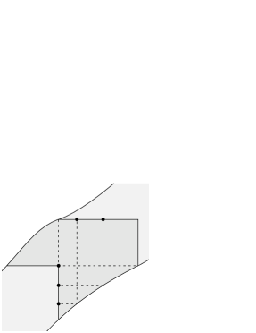
Figure 4.3. The case when two vertices of $R_{i-1}$ appear on $\partial_{*}\Omega_{t_{i}}$

Thus, we have found a sequence of elementary moves producing $R^{\prime}$ from $R$ in the case when $R\cap(\Omega_{0}\setminus\partial A)=\varnothing$.

4.3. The induction step

Suppose that $|R\cap(\Omega_{0}\setminus\partial A)|=m>0$ and the theorem is proved in the case when $|R\cap(\Omega_{0}\setminus\partial A)|<m$. We are going to find an elementary move $R\mapsto R_{1}$ performed inside $A$ such that $A$ is still suitable for defining a $\nearrow$-multiflype on $R_{1}$ (possibly after a small modification of $A$ not affecting the multiflype $R\mapsto R^{\prime}$), and $|R\cap(\Omega_{0}\setminus\partial A)|=m-1$. The induction step will then follow from Lemma 4.1.

Denote: $(\theta_{0},\varphi_{0})=u_{0}$, $(\theta_{1},\varphi_{1})=u_{1}=\overline{u}_{0}$. Let $v=(\theta_{2},\varphi_{2})$ be the closest to $u_{1}$ point in $R\cap(\Omega_{0}\setminus\partial A)$ (if there are more than one such point choose any of them). There are the following three cases to consider.

Case 1: $v\in r_{u_{0}}\setminus\partial r_{u_{0}}$. For $\varepsilon>0$, define $r(\varepsilon)$ to be the rectangle $[\theta_{2};\theta_{1}+\varepsilon]\times[\varphi_{2};\varphi_{1}+\varepsilon]$ (see the left picture in Figure 4.4).

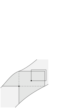
Figure 4.4. The rectangle $r(\varepsilon)$

For small enough $\varepsilon$, the following conditions hold:

1. the rectangle $r(\varepsilon)$ is contained in $A$;

2. $R\cap r(\varepsilon)=v$;

3. the meridian $m_{\theta_{1}+\varepsilon}$ and the longitude $\ell_{\varphi_{1}+\varepsilon}$ are disjoint from $R$.

Therefore, there is an elementary move $R\mapsto R_{1}$ performed inside $A$ such that $\sigma_{R_{1}}=\sigma_{R}-\sigma_{R}(v)\sigma_{r(\varepsilon)}$. We clearly have $|R_{1}\cap(\Omega_{0}\setminus\partial A)|=m-1$ as $v$ has been replaced by three vertices outside of $\Omega_{0}$.

By choosing $\varepsilon$ small enough we can also ensure that $A$ is still suitable to define a $\nearrow$-multiflype on $R_{1}$. Indeed, due to the nature of the conditions imposed on $A$, there are only finitely many $\varepsilon$ for which those conditions are violated.

Case 2: $v\in\Delta^{-}_{u_{0}}$. Denote $\theta_{3}=p_{\theta}(\overline{v})$. We define $r(\varepsilon)$ to be the rectangle $[\theta_{2};\theta_{3}]\times[\varphi_{2};\varphi_{1}+\varepsilon]$ (see the right picture in Figure 4.4) and proceed as in the previous case. A minor subtlety occurs only when $(\theta_{3},\varphi_{2})$ is not a vertex of $R$, in which case the diagram $R_{1}$ is forced to have an edge at the new meridian $m_{\theta_{3}}$, which does not depend on $\varepsilon$. This may result in failing of the last condition imposed on $A$ for defining a $\nearrow$-multiflype on $R_{1}$.

However, this is easily resolved by a small perturbation of $\partial A$ near the intersections with $m_{\theta_{3}}$ other than $(\theta_{3},\varphi_{2})$. Such perturbations do not affect the flype $R\mapsto R^{\prime}$, since these points are not contained in any longitude or meridian passing through a vertex of $R$.

Case 3: $v\in\Delta^{+}_{u_{0}}$. This case is symmetric to the previous one and left to the reader.

The proof of Theorem 2.1 is now complete.

5. Concluding remarks

By a $\diagup$-multiflype (respectively, a $\diagdown$-multiflype) we call any $\nearrow$- or $\swarrow$-multiflype (respectively, $\nwarrow$- or $\searrow$-multiflype).

The proof of Theorem 2.1 given above provides an algorithm for decomposing any multiflype into a sequence of elementary moves. By following the lines of the proof one can see that the decomposition of a $\diagup$-multiflype consists of elementary moves that are particular cases of $\diagup$-multiflypes. Similarly for $\diagdown$-multiflypes.

Any exchange move (or commutation) of rectangular diagrams of links can be simultaneously viewed as a $\diagup$-multiflype and a $\diagdown$-multiflype.

Stabilizations and destabilization which are $\diagup$-multiflypes are exactly those that are called type I (de)stabilization in [4]. In the terminology of [9], these are (de)stabilizations of types X:NE, X:SW, O:NE, and O:SW. Similarly, (de)stabilizations which are $\diagdown$-multiflypes are those that are of type II in [4] and of types X:NW, X:SE, O:NW, and O:SE in [9].

With every rectangular diagram of a link $R$, one associates two Legendrian link types, one with respect to the standard contact structure $\xi_{\mathrm{st}}$, and the other with respect to the mirror image of $\xi_{\mathrm{st}}$ (see [4, 9]). We denote them here by $\mathscr{L}_{\diagup}(R)$ and $\mathscr{L}_{\diagdown}(R)$, respectively.

Due to the remark above the relation between rectangular diagrams of links and Legendrian links, which is explained in [4, 9], can be summarized as follows.

Corollary 5.1.

Let $R_{1}$ and $R_{2}$ be oriented rectangular diagrams of links. We have $\mathscr{L}_{\diagup}(R_{1})=\mathscr{L}_{\diagup}(R_{2})$ (respectively, $\mathscr{L}_{\diagdown}(R_{1})=\mathscr{L}_{\diagdown}(R_{2})$) if and only if $R_{1}$ and $R_{2}$ are related by a sequence of $\diagup$-multiflypes (respectively, $\diagdown$-multiflypes).

In [10], flypes of rectangular diagrams of links are generalized to the case of rectangular diagrams of graphs. One can similarly generalize multiflypes and Theorem 2.1 for general graphs, as well as Corollary 5.1 for Legendrian graphs, and the proof will need no essential change.

References

- [1] P. R. Cromwell. Embedding knots and links in an open book. I. Basic properties. Topology Appl. 64 (1995), no. 1, 37–58.
- [2] I. Dynnikov. Recognition algorithms in knot theory. (Russian) Uspekhi Mat. Nauk 58 (2003), no. 6 (354), 45–92; translation in Russian Math. Surveys 58 (2003), no. 6, 1093–1139.
- [3] I. Dynnikov. Arc-presentations of links: Monotonic simplification. Fund. Math. 190 (2006), 29–76; arXiv:math/0208153.
- [4] I. Dynnikov, M. Prasolov. Bypasses for rectangular diagrams. A proof of the Jones conjecture and related questions (Russian), Trudy MMO 74 (2013), no. 1, 115–173; translation in Trans. Moscow Math. Soc. 74 (2013), no. 2, 97–144; arXiv:1206.0898.
- [5] W. Jaco, J. Tollefson. Algorithms for the complete decomposition of a closed 3-manifold. Illinois J. Math. 39 (1995), no. 3, 358–406.
- [6] W. Jaco, D. Letscher, H. J. Rubinstein. Algorithms for essential surfaces in 3-manifolds. Topology and geometry: commemorating SISTAG, 107–124, Contemp. Math., 314, Amer. Math. Soc., Providence, RI, 2002.
- [7] W. Haken. Theorie der Normalflächen. (German) Acta Math. 105 (1961), 245–375.
- [8] A. Kazantsev. The problem of detecting the satellite structure of a link by monotonic simplification. J. Knot Theory Ramifications 20 (2011), no. 1, 109–125; arXiv:1005.5263.
- [9] P.Ozsváth, Z.Szabó, D.Thurston. Legendrian knots, transverse knots and combinatorial Floer homology, Geometry and Topology, 12 (2008), 941–980; arXiv:math/0611841.
- [10] M. Prasolov. Rectangular diagrams of Legendrian graphs. J. Knot Theory Ramifications 23 (2014), no. 13, 1450074; arXiv:1412.2267.
- [11] H. Schubert. Bestimmung der Primfaktorzerlegung von Verkettungen. (German) Math. Z. 76 (1961), 116–148.