Chaotic dynamics of a three particle array under Lennard–Jones type forces and a fixed area constraint

Abstract

We consider the dynamical problem for a system of three particles in which the inter–particle forces are given as the gradient of a Lennard–Jones type potential. Furthermore we assume that the three particle array is subject to the constraint of fixed area. The corresponding mathematical problem is that of a conservative dynamical system over the manifold determined by the area constraint. We study numerically the stability of this system. In particular, using the recently introduced measure of chaos by Hunt and Ott (2015), we study numerically the possibility of chaotic behaviour for this system.

Keywords: dynamical system, chaos, expansion entropy, constrained optimization

AMS subject classifications: 70H45, 37M05, 37D45

1 Introduction

In this paper we consider the dynamical problem for a system of three particles, where the interactions between the particles of the system are due to forces given as the gradient of a Lennard–Jones [12] type potential. Furthermore we assume that the three particle array is subjected to the additional constraint that the area of the triangle generated by them is fixed. The motivation to consider the area constraint comes from the following phenomena observed both in laboratory experiments and molecular dynamics simulations (see e.g., [1, 2]). As the density of a fluid is progressively lowered (keeping the temperature constant), there is a certain “critical” density such that if the density of the fluid is lower than this critical value, then bubbles or regions with very low density appear within the fluid. This phenomenon is usually called “cavitation” and it has been extensively studied as well in solids. (See for instance [4, 9] for discussions and further references.)

The dynamical system under consideration in this paper is an example of a conservative dynamical system over a manifold (cf. (2.7)). The numerical techniques to compute approximate solutions for these types of problems are based essentially on variations of a predictor–corrector (or projection) method. We refer to [5], [6] for a discussion on the existence and uniqueness, dependence on initial data, as well as numerical schemes for general dynamical systems over manifolds. The assumptions that one particle is fixed at the origin and that another one moves along one of the coordinate axes, simplify greatly the area constraint in our problem. Using this we show in Section 4 that our original constrained dynamical system reduces to a standard (non-constrained) dynamical system (cf. (4.3)) involving the area parameter.

In Section 3 we give a characterization of the equilibrium points of (2.7) or equivalently (4.3). We show that these equilibrium points coincide with those studied in [14]. In that paper the equilibrium problem is treated as a bifurcation problem with the specified area as the bifurcation parameter. They showed the existence of a family of equilibrium states corresponding to equilateral triangles, and that these equilibrium points are stable up to a certain critical area $A_{c}$ after which they become unstable. Furthermore, using techniques of equivariant bifurcation theory they showed that bifurcating from the point corresponding to $A_{c}$, there are solutions curves corresponding to isosceles triangles the stability of which could only be determined numerically. Moreover for an instance of the Lennard–Jones potential, they showed numerically that stable equilibrium points corresponding to scalene triangles exist for a range of values of the area parameter.

The study of chaotic behaviour in dynamical systems is a very important and active area in this field. Verifying whether or not a particular system is chaotic can be a difficult task. In Section 5 we review a new criteria for chaos introduced recently by Hunt and Ott [10]. This new characterization of chaos is based on the so called expansion entropy (cf. (5.5)) which does not require the identification of a compact invariant set, and naturally leads itself to a computational method for detecting chaotic behaviour in a dynamical system. In Section 5 we describe this numerical scheme and give several examples of the use of this method applied to various dynamical systems of known chaotic or non–chaotic behaviour. Finally in Section 6 we use this method to show that the dynamical system for the three particle array under the area constraint, exhibits chaotic behaviour essentially for all values of the area parameter in the area constraint.

2 Problem formulation

We consider a system of three equal particles interacting via an inter–particle potential $\phi$. The potentials we are concerned are those of the form:

$$\phi(r)=\dfrac{c_{1}}{r^{\delta_{1}}}-\dfrac{c_{2}}{r^{\delta_{2}}},$$ (2.1)

where $c_{1},c_{2}$ are positive constants and $\delta_{1}>\delta_{2}>2$. These constants determine the physical properties of the particles or molecules in the array. (The classical Lennard–Jones [12] potential is obtained upon setting $\delta_{1}=12$ and $\delta_{2}=6$.) We study the planar dynamics of such a system subject to the constraint of fixed area for the triangular array.

Let $\mathbf{r}_{i}(t)$, $i=1,2,3$ be the position vectors of the particles, and $\mathbf{r}_{ij}(t)=\mathbf{r}_{i}(t)-\mathbf{r}_{j}(t)$ for $i<j$. Let

$$r_{i}=||\mathbf{r}_{i}||=(\mathbf{r}_{i}\cdot\mathbf{r}_{i})^{\frac{1}{2}},\quad r_{ij}=||\mathbf{r}_{ij}||.$$

If $m$ is the particle mass, then the kinetic and potential energies of the system are given respectively by:

$$K=\frac{m}{2}\sum_{i=1}^{3}||\dot{\mathbf{r}}_{i}||^{2},\quad U=\sum_{i<j}\phi(r_{ij}).$$ (2.2)

Thus we seek to minimize the Lagrangian $L=K-U$ over the time interval $[0,t_{f}]$ which leads us to consider the functional:

$$E(\mathbf{r}_{1},\mathbf{r}_{2},\mathbf{r}_{3})=\int_{0}^{t_{f}}(K-U)\,\mathrm{d}t$$

The square of the area of a triangle with sides $a,b,c$ is given according to Heron’s formula by

$$\Gamma(a,b,c)=\frac{1}{8}(a^{2}b^{2}+a^{2}c^{2}+b^{2}c^{2})-\frac{1}{16}(a^{4}+b^{4}+c^{4}).$$ (2.3)

For any $A>0$ we let

$$g(\mathbf{r}_{1},\mathbf{r}_{2},\mathbf{r}_{3})=\Gamma(r_{12},r_{13},r_{23})-A^{2}.$$ (2.4)

Thus if we set $g=0$, then we would be specifying that the triangle defined by the positions of the three particles is of fixed area $A$. We shall need the following formulas for the partial derivatives of $g$:

$$\frac{\partial g}{\partial\mathbf{r}_{1}} = \dfrac{1}{r_{12}}\,\frac{\partial\Gamma}{\partial a}(\mathbf{r}_{1}-\mathbf{r}_{2})+\dfrac{1}{r_{13}}\,\frac{\partial\Gamma}{\partial b}(\mathbf{r}_{1}-\mathbf{r}_{3}),$$ (2.5a)

$$\frac{\partial g}{\partial\mathbf{r}_{2}} = -\dfrac{1}{r_{12}}\,\frac{\partial\Gamma}{\partial a}(\mathbf{r}_{1}-\mathbf{r}_{2})+\dfrac{1}{r_{23}}\,\frac{\partial\Gamma}{\partial c}(\mathbf{r}_{2}-\mathbf{r}_{3}),$$ (2.5b)

$$\frac{\partial g}{\partial\mathbf{r}_{3}} = -\dfrac{1}{r_{13}}\,\frac{\partial\Gamma}{\partial b}(\mathbf{r}_{1}-\mathbf{r}_{3})-\dfrac{1}{r_{23}}\,\frac{\partial\Gamma}{\partial c}(\mathbf{r}_{2}-\mathbf{r}_{3}),$$ (2.5c)

where the partial derivatives of $\Gamma$ are evaluated at $(r_{12},r_{13},r_{23})$. Note that

$$\frac{\partial g}{\partial\mathbf{r}_{1}}+\frac{\partial g}{\partial\mathbf{r}_{2}}+\frac{\partial g}{\partial\mathbf{r}_{3}}=\mathbf{0}.$$ (2.6)

2.1 The constrained problem

We assume that the particle corresponding to $i=3$ is fixed at the origin, while that for $i=2$ is restricted to move along the $x$–axis. Using the notation $\mathbf{r}_{i}=(u_{i},w_{i})$, $i=1,2,3$, our variational problem becomes that of finding $C^{1}$ functions $\mathbf{r}_{1},\mathbf{r}_{2},\mathbf{r}_{3}$ such that:

$$\begin{array}[]{c}\min~{}E(\mathbf{r}_{1},\mathbf{r}_{2},\mathbf{r}_{3})\\ \mbox{subject~{}to~{}}g(\mathbf{r}_{1},\mathbf{r}_{2},\mathbf{r}_{3})=0,\quad\mathbf{r}_{3}=\mathbf{0},\quad w_{2}=0.\end{array}$$

The Euler–Lagrange equations for the above variational problem are given by:

$$m\ddot{\mathbf{r}}_{1} = -\dfrac{\phi^{\prime}(r_{12})}{r_{12}}(\mathbf{r}_{1}-\mathbf{r}_{2})-\dfrac{\phi^{\prime}(r_{13})}{r_{13}}(\mathbf{r}_{1}-\mathbf{r}_{3})-\lambda\frac{\partial g}{\partial\mathbf{r}_{1}}(\mathbf{r}_{1},\mathbf{r}_{2},\mathbf{r}_{3}),$$

$$m\ddot{\mathbf{r}}_{2} = \dfrac{\phi^{\prime}(r_{12})}{r_{12}}(\mathbf{r}_{1}-\mathbf{r}_{2})-\dfrac{\phi^{\prime}(r_{23})}{r_{23}}(\mathbf{r}_{2}-\mathbf{r}_{3})-\lambda\frac{\partial g}{\partial\mathbf{r}_{2}}(\mathbf{r}_{1},\mathbf{r}_{2},\mathbf{r}_{3})-\mu\mathbf{e}_{2},$$ (2.7)

$$m\ddot{\mathbf{r}}_{3} = \dfrac{\phi^{\prime}(r_{13})}{r_{13}}(\mathbf{r}_{1}-\mathbf{r}_{3})+\dfrac{\phi^{\prime}(r_{23})}{r_{23}}(\mathbf{r}_{2}-\mathbf{r}_{3})-\lambda\frac{\partial g}{\partial\mathbf{r}_{3}}(\mathbf{r}_{1},\mathbf{r}_{2},\mathbf{r}_{3})-\nu_{1}\mathbf{e}_{1}-\nu_{2}\mathbf{e}_{2},$$

$$0 = g(\mathbf{r}_{1},\mathbf{r}_{2},\mathbf{r}_{3}),\quad\mathbf{r}_{3}=\mathbf{0},\quad w_{2}=0.$$

Here $\lambda$, $\nu_{1},\nu_{2},\mu$ (which are functions of $t$) are the Lagrange multipliers corresponding to the constraints in the problem, and $\left\{\mathbf{e}_{1},\mathbf{e}_{2}\right\}$ is the standard basis for $\mathbb{R}^{2}$. From these equations and (2.6), it follows now that

$$m\sum_{i=1}^{3}\ddot{\mathbf{r}}_{i}(t)=-\nu_{1}\mathbf{e}_{1}-(\nu_{2}+\mu)\mathbf{e}_{2},$$

which describes the motion of the center of mass of the system. The system (2.7) is conservative as the energy $K+U$ is conserved along solutions.

Applying the constraints $\mathbf{r}_{3}=\mathbf{0}$ and $w_{2}=0$, the equations above simplify to:

$$m\ddot{\mathbf{r}}_{1} = -\dfrac{\phi^{\prime}(r_{12})}{r_{12}}(\mathbf{r}_{1}-\mathbf{r}_{2})-\dfrac{\phi^{\prime}(r_{1})}{r_{1}}\mathbf{r}_{1}-\lambda\frac{\partial g}{\partial\mathbf{r}_{1}},$$

$$m\ddot{u}_{2} = \dfrac{\phi^{\prime}(r_{12})}{r_{12}}(u_{1}-u_{2})-\dfrac{\phi^{\prime}(r_{2})}{r_{2}}u_{2}-\lambda\frac{\partial g}{\partial u_{2}},$$

$$0 = \dfrac{\phi^{\prime}(r_{12})}{r_{12}}w_{1}-\lambda\frac{\partial g}{\partial w_{2}}-\mu,$$

$$\mathbf{0} = \dfrac{\phi^{\prime}(r_{1})}{r_{1}}\mathbf{r}_{1}+\dfrac{\phi^{\prime}(r_{2})}{r_{2}}\mathbf{r}_{2}-\lambda\frac{\partial g}{\partial\mathbf{r}_{3}}-\nu_{1}\mathbf{e}_{1}-\nu_{2}\mathbf{e}_{2},$$

$$0 = g.$$

where $g$ and all of its partial derivatives are evaluated at $(u_{1},w_{1},u_{2},0,0,0)$. Note that since $r_{2}=|u_{2}|$, the first two equations together with the last one, can be solved independently of the third and fourth equations. Once $\mathbf{r}_{1}$, $u_{2}$, and $\lambda$ are determined, one can find $\nu_{1},\nu_{2},\mu$ using the third and fourth equations. Thus we are lead to consider the system in component form:

$$m\ddot{u}_{1} = -\dfrac{\phi^{\prime}(r_{12})}{r_{12}}(u_{1}-u_{2})-\dfrac{\phi^{\prime}(r_{1})}{r_{1}}u_{1}-\lambda\frac{\partial\gamma}{\partial u_{1}}(u_{1},w_{1},u_{2}),$$

$$m\ddot{w}_{1} = -\left[\dfrac{\phi^{\prime}(r_{12})}{r_{12}}+\dfrac{\phi^{\prime}(r_{1})}{r_{1}}\right]w_{1}-\lambda\frac{\partial\gamma}{\partial w_{1}}(u_{1},w_{1},u_{2}),$$ (2.8)

$$m\ddot{u}_{2} = \dfrac{\phi^{\prime}(r_{12})}{r_{12}}(u_{1}-u_{2})-\dfrac{\phi^{\prime}(r_{2})}{r_{2}}u_{2}-\lambda\frac{\partial\gamma}{\partial u_{2}}(u_{1},w_{1},u_{2}),$$

$$0 = \gamma(u_{1},w_{1},u_{2}),$$

where $\gamma(u_{1},w_{1},u_{2})=g(u_{1},w_{1},u_{2},0,0,0)$.

We recall that in these equations

$$r_{12}=\sqrt{(u_{1}-u_{2})^{2}+w_{1}^{2}},\quad r_{1}=\sqrt{u_{1}^{2}+w_{1}^{2}},\quad r_{2}=|u_{2}|.$$ (2.9)

It is easy to check now that

$$\gamma(u_{1},w_{1},u_{2})=\frac{1}{4}w_{1}^{2}u_{2}^{2}-A^{2}.$$

Thus the area constraint $\gamma=0$ is simply the square of the familiar formula of “area equals one half base times height”. We shall exploit this very shortly but before doing so, we pause to characterize the equilibrium points of the system (2.8).

3 The equilibrium points

We now show that the equilibrium points of the system (2.8) are precisely those studied in [14]. We remark that while $\lambda$ in (2.8) is in general a function of $t$, in the following discussion it is a constant corresponding to a steady state.

Proposition 3.1.

The equilibrium points of the system (2.8) correspond to position vectors $\mathbf{r}_{1}=(u_{1},w_{1})$ and $\mathbf{r}_{2}=(u_{2},0)$ for which $a=r_{12}$, $b=r_{1}$, and $c=r_{2}$ (cf. (2.3), (2.9)) satisfy:

$$\left\{\begin{array}[]{rcl}\phi^{\prime}(a)+\lambda\Gamma_{,a}&=&0,\\ \phi^{\prime}(b)+\lambda\Gamma_{,b}&=&0,\\ \phi^{\prime}(c)+\lambda\Gamma_{,c}&=&0,\\ \Gamma(a,b,c)&=&A^{2},\end{array}\right.$$ (3.1)

where $\Gamma_{,a}=\frac{\partial\Gamma}{\partial a}$, etc.

Proof: After setting the right hand side of (2.8) equal to zero, we are led to

$$\dfrac{\phi^{\prime}(a)}{a}(u_{1}-u_{2})+\dfrac{\phi^{\prime}(b)}{b}u_{1}+\lambda\frac{\partial\gamma}{\partial u_{1}} = 0,$$ (3.2a)

$$\dfrac{\phi^{\prime}(a)}{a}w_{1}+\dfrac{\phi^{\prime}(b)}{b}w_{1}+\lambda\frac{\partial\gamma}{\partial w_{1}} = 0,$$ (3.2b)

$$-\dfrac{\phi^{\prime}(a)}{a}(u_{1}-u_{2})+\dfrac{\phi^{\prime}(c)}{c}u_{2}+\lambda\frac{\partial\gamma}{\partial u_{2}} = 0,$$ (3.2c)

$$\gamma(u_{1},w_{1},u_{2}) = 0,$$ (3.2d)

where we have set $a=r_{12}$, $b=r_{1}$, and $c=r_{2}$. The constraint $\gamma(u_{1},w_{1},u_{2})=0$ is equivalent to $\Gamma(a,b,c)=A^{2}$. Since $A>0$ is the area of the triangle determined by $\mathbf{r}_{1}=(u_{1},w_{1})$, $\mathbf{r}_{2}=(u_{2},0)$, and the origin, it follows that

$$w_{1}\neq 0,\quad u_{2}\neq 0.$$

Now using that $w_{2}=0$ and $\mathbf{r}_{3}=\mathbf{0}$ together with the definitions of $a,b,c$, we get from (2.5a) and the first component of (2.5b) that:

$$\frac{\partial\gamma}{\partial u_{1}} = \dfrac{1}{a}\,\Gamma_{,a}(u_{1}-u_{2})+\dfrac{1}{b}\,\Gamma_{,b}u_{1},$$

$$\frac{\partial\gamma}{\partial w_{1}} = \dfrac{1}{a}\,\Gamma_{,a}w_{1}+\dfrac{1}{b}\,\Gamma_{,b}w_{1},$$

$$\frac{\partial\gamma}{\partial u_{2}} = -\dfrac{1}{a}\,\Gamma_{,a}(u_{1}-u_{2})+\dfrac{1}{c}\,\Gamma_{,c}u_{2}.$$

If we now substitute these equations into (3.2), and add and subtract (3.2a) and (3.2c), then the first three equations of (3.2) are equivalent to:

$$H_{b}u_{1}+H_{c}u_{2} = 0,$$

$$(2H_{a}+H_{b})u_{1}-(2H_{a}+H_{c})u_{2} = 0,$$ (3.3)

$$(H_{a}+H_{b})w_{1} = 0,$$

where

$$H_{a}=\frac{1}{a}\left(\phi^{\prime}(a)+\lambda\Gamma_{,a}\right),\mbox{ etc.}$$

Since $w_{1}\neq 0$ we must have that $H_{a}=-H_{b}$. Since $u_{2}\neq 0$ the determinant of the coefficient matrix of the first two equations in the system (3.3) must be zero. A calculation shows that this determinant is $2H_{a}^{2}$. Hence $H_{a}=0$, and since $H_{b}=-H_{a}$, then $H_{b}=0$. It follows now from the first equation of (3.3) and using that $u_{2}\neq 0$, that $H_{c}=0$. Since $H_{a}=H_{b}=H_{c}=0$ is equivalent to the first three equations in (3.1), the result follows. ∎
For future reference we record here the basic result in [14] concerning the existence and multiplicity of solutions of the system (3.1).

Theorem 3.2.

For any value of $A>0$, the system (3.1) has a solution of with $a=b=c=a_{A}$ corresponding to an equilateral triangle with corresponding Lagrange–multiplier $\lambda_{A}$ where:

$$a_{A}=\frac{2\sqrt{A}}{\sqrt[4]{3}},\quad\lambda_{A}=-\frac{4\phi^{\prime}(a_{A})}{a_{A}^{3}}.$$ (3.4)

This equilibrium point is stable, that is, a minimizer of the potential energy functional $U$ in (2.2) subject to the fixed area constraint, if and only if

$$\rho(A)\equiv\phi^{\prime\prime}(a_{A})+\frac{3}{a_{A}}\phi^{\prime}(a_{A})>0.$$ (3.5)

Moreover, if $A_{0}$ is a simple root of $\rho(\cdot)$, then there exist three branches of solutions corresponding to isosceles triangles, bifurcating from the branch of equilateral triangles at the point where $A=A_{0}$.

The stability of the bifurcating branches in Theorem 3.2 can only be determined numerically. In [14] they give numerical examples in which these bifurcations are of the trans–critical type and also that there can be secondary bifurcations into stable scalene triangles.

4 The reduced problem

The system (2.8) is an example of a dynamical system over a manifold. One can in principle solve this system directly using some of the numerical techniques for these types of problems, that essentially are based on variations of a predictor–corrector (or projection) method (cf. [5], [6]). However because of the simplification of the constraint $\gamma=0$ in (2.8), the system (2.8) can be reduced further to one in the variables $(u_{1},w_{1})$. This simplifies greatly the calculations in Section 6 when we apply to our problem the new criteria for detecting chaos in [10].

As we mentioned before, the constraint $\gamma=0$ reduces to:

$$\frac{1}{4}w_{1}^{2}u_{2}^{2}-A^{2}=0,$$

Since $w_{1}\neq 0$ and $u_{2}\neq 0$ and $A>0$, we may assume that $w_{1}>0$ and $u_{2}>0$. It follows now that

$$\frac{\partial\gamma}{\partial u_{1}}=0,\quad\frac{\partial\gamma}{\partial w_{1}}=\frac{1}{2}w_{1}u_{2}^{2},\quad\frac{\partial\gamma}{\partial u_{2}}=\frac{1}{2}w_{1}^{2}u_{2}.$$ (4.1)

Using these and the fact that the constraint $\gamma=0$ is equivalent to $w_{1}u_{2}=2A$, we can eliminate $\lambda$ and the equation of $u_{2}$ from (2.8), to get the following reduced system for $u_{1},w_{1}$:

$$m\ddot{u}_{1} = -\dfrac{\phi^{\prime}(r_{12})}{r_{12}}(u_{1}-u_{2})-\dfrac{\phi^{\prime}(r_{1})}{r_{1}}u_{1},$$ (4.2a)

$$m\left[w_{1}^{2}+u_{2}^{2}\right]\ddot{w}_{1} = 2A\left[-\dfrac{\phi^{\prime}(r_{12})}{r_{12}}(u_{1}-u_{2})+\phi^{\prime}(u_{2})\right]$$ (4.2b)

$$-\left[\dfrac{\phi^{\prime}(r_{12})}{r_{12}}+\dfrac{\phi^{\prime}(r_{1})}{r_{1}}\right]w_{1}^{3}+8mA^{2}\dfrac{(\dot{w}_{1})^{2}}{w_{1}^{3}}.$$

In these equations $w_{1}>0$ and any instance of $u_{2}$ should be replaced with $2A/w_{1}$.

For the numerical calculations of the next section, we shall need to transform the system (4.2) into one of first order. If we let $v_{1}=\dot{u}_{1}$ and $v_{2}=\dot{w}_{1}$, then the above system is equivalent to:

$$\dot{u}_{1} = v_{1},\quad\dot{w}_{1}=v_{2},$$

$$m\dot{v}_{1} = -\dfrac{\phi^{\prime}(r_{12})}{r_{12}}(u_{1}-u_{2})-\dfrac{\phi^{\prime}(r_{1})}{r_{1}}u_{1},$$ (4.3a)

$$m\left[w_{1}^{2}+u_{2}^{2}\right]\dot{v}_{2} = 2A\left[-\dfrac{\phi^{\prime}(r_{12})}{r_{12}}(u_{1}-u_{2})+\phi^{\prime}(u_{2})\right]$$ (4.3b)

$$-\left[\dfrac{\phi^{\prime}(r_{12})}{r_{12}}+\dfrac{\phi^{\prime}(r_{1})}{r_{1}}\right]w_{1}^{3}+8mA^{2}\dfrac{v_{2}^{2}}{w_{1}^{3}}.$$

Given any $(p,q,\alpha,\beta)$ with $q>0$, it follows from the standard existence and uniqueness theorem for ode’s that these equations have a unique solution satisfying

$$u_{1}(0)=p,\quad w_{1}(0)=q,\quad v_{1}(0)=\alpha,\quad v_{2}(0)=\beta.$$

If we let $\mathbf{r}=(u_{1},w_{1},v_{1},v_{2})$ and $\mathbf{p}=(p,q,\alpha,\beta)$, then we shall write $\mathbf{r}(t;\mathbf{p})$ to denote the dependence of the solution of (4.3) on the initial conditions $\mathbf{p}$. It follows from standard results on the dependence on initial values for the solutions of initial value problems (cf. [7]), that $\mathbf{r}(t;\mathbf{p})$ is a differentiable function of $\mathbf{p}$.

5 A criteria for chaos

The study of chaotic behaviour in dynamical systems is a very important and active area in this field. A commonly used definition of chaos, originally formulated by Robert L. Devaney, says that for a dynamical system to be classified as chaotic, it must have the following properties [8]:

• it must be sensitive to initial conditions

• it must be topologically mixing

• it must have dense periodic orbits

Verifying whether these properties hold or not for a particular system can be a difficult task. Recently Hunt and Ott [10] developed a new criteria for chaos based on the so called expansion entropy (cf. (5.5)) which does not require the identification of a compact invariant set. In this section we introduce some of the notions and definitions in [10] leading to a practical, from the numerical point of view, characterization of chaos for a dynamical system.

We consider an autonomous dynamical system of the form:

$$\dot{\mathbf{r}}(t)=\mathbf{f}(\mathbf{r}(t)),$$ (5.1)

where $\mathbf{f}:\Omega\rightarrow\mathbb{R}^{n}$ is a smooth function, and $\Omega\subset\mathbb{R}^{n}$ is open with a smooth boundary. We denote by $\mathbf{r}(\cdot;\mathbf{p})$ the solution of (5.1) such that $\mathbf{r}(0)=\mathbf{p}$. $\mathbf{r}(\cdot;\mathbf{p})$ is called the flow or evolution operator of (5.1). Let

$$\mathbf{u}(\cdot;\mathbf{p})=\mathrm{D}_{\mathbf{p}}\mathbf{r}(\cdot;\mathbf{p}).$$ (5.2)

Note that $\mathbf{u}(t;\mathbf{p})$ is an $n\times n$ matrix for each $t$. Now since $\mathbf{r}(0;\mathbf{p})=\mathbf{p}$, it follows that $\mathbf{u}(0;\mathbf{p})=\mathbf{I}$, where $\mathbf{I}$ is the $n\times n$ identity matrix. After differentiating in (5.1) with respect to $\mathbf{p}$, we get that

$$\dot{\mathbf{u}}(t)=\mathrm{D}_{\mathbf{r}}\mathbf{f}(\mathbf{r}(t))\mathbf{u}(t).$$

Thus, the flow $\mathbf{r}(\cdot;\mathbf{p})$ and the matrix function $\mathbf{u}(\cdot;\mathbf{p})$ are solutions of the initial value problem:

$$\dot{\mathbf{u}}(t) = \mathrm{D}_{\mathbf{r}}\mathbf{f}(\mathbf{r}(t))\mathbf{u}(t),$$ (5.3a)

$$\dot{\mathbf{r}}(t) = \mathbf{f}(\mathbf{r}(t)),$$ (5.3b)

$$\mathbf{u}(0) = \mathbf{I},\quad\mathbf{r}(0)=\mathbf{p}.$$ (5.3c)

The function $\mathbf{u}$ is central in the definition of chaos in [10]. In particular, let $G(\mathbf{u})$ be the product of the singular values of $\mathbf{u}$ that are greater than $1$. (If none of the singular values are greater than $1$, we set $G(\mathbf{u})=1$.) For any subset $S$ of $\Omega$, called a restraining region, let

$$S_{T}=\left\{\mathbf{p}\in S\,:\,\mathbf{r}(t;\mathbf{p})\in S,\quad t\in[0,T]\right\},$$

and define

$$E_{T}(\mathbf{r},S)=\frac{1}{|S|}\int_{S_{T}}G(\mathbf{u}(T;\mathbf{p}))\,\mathrm{d}\mathbf{p},$$ (5.4)

where $|S|$ is the volume of $S$. The expansion entropy $H_{0}(\mathbf{r},S)$ of the flow $\mathbf{r}$ over the set $S$ is defined as:

$$H_{0}(\mathbf{r},S)=\lim_{T\rightarrow\infty}\dfrac{\ln E_{T}(\mathbf{r},S)}{T}.$$ (5.5)

According to [10] the system (5.1) is chaotic if for some restraining region $S$, we have that $H_{0}(\mathbf{r},S)>0$.

Remark 5.1.

The expansion entropy function has several nice properties, one of them being that $H_{0}(\mathbf{r},S^{\prime})\leq H_{0}(\mathbf{r},S)$ whenever $S^{\prime}\subset S$. Thus if chaos is detected for any region $S^{\prime}$, it will also be detected for any other region containing $S^{\prime}$.

Remark 5.2.

The definitions in this section can be extended to non–autonomous systems and for any manifold $\Omega$ in $\mathbb{R}^{n}$ (cf. [10]).

Example 5.3.

We consider the constant coefficient linear system

$$\dot{\mathbf{r}}(t)=A\mathbf{r}(t),$$ (5.6)

where $A$ is an $n\times n$ matrix. The solution of this system is given by

$$\mathbf{r}(t)=\mathrm{e}^{tA}\mathbf{p},\quad t\in\mathbb{R},$$

where $\mathbf{p}\in\mathbb{R}^{n}$ is arbitrary. Here

$$\mathrm{e}^{tA}=\sum_{k=0}^{\infty}\frac{t^{k}}{k!}\,A^{k}.$$

It follows from the above representation of the solution $\mathbf{r}(\cdot)$ that the linear dynamical system above is non chaotic. We show now that the definition of chaos in [10] gives indeed a non chaotic behaviour in this case.

For simplicity of exposition we assume that $A$ is symmetric with eigenvalues $\lambda_{1}\leq\lambda_{2}\leq\cdots\leq\lambda_{n}$ and corresponding orthonormal eigenvectors $\left\{\mathbf{x}_{1},\mathbf{x}_{2},\ldots,\mathbf{x}_{n}\right\}$. In this case, the matrix $\mathrm{e}^{tA}$ is symmetric as well with eigenvalues $\mathrm{e}^{\lambda_{1}t}$, $\mathrm{e}^{\lambda_{2}t}$,…,$\mathrm{e}^{\lambda_{n}t}$ with the same corresponding eigenvectors as $A$. Since the eigenvalues of $\mathrm{e}^{tA}$ are all positive, it follows that the singular values of $\mathrm{e}^{tA}$ coincide with its eigenvalues. Since the matrix $\mathbf{u}$ in (5.2) is given by $\mathrm{e}^{tA}$, we get that

$$G(\mathbf{u}(t;\mathbf{p}))=\mathrm{e}^{t\sum_{\lambda_{i}>0}\lambda_{i}},$$

or one if the sum in the exponent is empty. In particular $G(\mathbf{u}(t;\mathbf{p}))$ is independent of $\mathbf{p}$.

Writing $\mathbf{p}=\sum_{i=1}^{n}c_{i}\mathbf{x}_{i}$, we get that

$$\mathbf{r}(t)=\sum_{i=1}^{n}c_{i}\mathrm{e}^{\lambda_{i}t}\mathbf{x}_{i}.$$

For the restraining region, we consider the set

$$S=\left\{\mathbf{p}=\sum_{i=1}^{n}c_{i}\mathbf{x}_{i}\,:\,\left|c_{i}\right|\leq a\right\},$$

for any $a>0$. If all $\lambda_{i}$ are nonpositive, then $S_{T}=S$, $G(\mathbf{u}(T;\mathbf{p}))=1$, and we get that $E_{T}(\mathbf{r},S)=1$, and thus that $H_{0}(\mathbf{r},S)=0$.

Assume now that there are $p>0$ positive eigenvalues $\lambda_{i}$. In this case

$$S_{T}=\left\{\sum_{i=1}^{n}c_{i}\mathbf{x}_{i}\,:\,\left|c_{i}\right|\leq a,\,1\leq i\leq n-p,\quad\left|c_{i}\right|\leq a\mathrm{e}^{-\lambda_{i}T},\,n-p+1\leq i\leq n\right\},$$

and $G(\mathbf{u}(T;\mathbf{p}))=\mathrm{e}^{T\sum_{i=n-p+1}^{n}\lambda_{i}}$. As $\left|S_{T}\right|=(2a)^{n}\mathrm{e}^{-T\sum_{i=n-p+1}^{n}\lambda_{i}}$, we get that

$$E_{T}(\mathbf{r},S) = \frac{1}{|S|}\int_{S_{T}}G(\mathbf{u}(T;\mathbf{p}))\,\mathrm{d}\mathbf{p},$$

$$= \frac{1}{(2a)^{n}}G(\mathbf{u}(T;\mathbf{p}))\left|S_{T}\right|=1.$$

Once again we get that that $H_{0}(\mathbf{r},S)=0$.

For an arbitrary compact restraining region $S^{\prime}$, we take $a$ in the definition of $S$ above sufficiently large such that $S^{\prime}\subset S$. It follows from Remark 5.1 that $H_{0}(\mathbf{r},S^{\prime})\leq H_{0}(\mathbf{r},S)=0$, and thus that the linear dynamical system is non chaotic according to [10].

The definition of $H_{0}(\mathbf{r},S)$ given in this section leads naturally to a very practical numerical scheme for estimating this quantity and thus to numerically test for chaos for a given dynamical system. If we take a set $\left\{\mathbf{p}_{1},\ldots,\mathbf{p}_{N}\right\}$ of uniformly random vectors in $S$, then we can approximate (5.4) by $\hat{E}_{T}(\mathbf{r},S)$ were

$$\hat{E}_{T}(\mathbf{r},S)=\dfrac{1}{N}\sum_{{k=1}\atop{\mathbf{p}_{k}\in S_{T}}}^{N}G(\mathbf{u}(T;\mathbf{p}_{k})).$$ (5.7)

This sum is computed for different values of $T\in[0,T_{\mbox{max}}]$ for some prescribed $T_{\mbox{max}}$. The whole computation is repeated for different random samples of the $\left\{\mathbf{p}_{1},\ldots,\mathbf{p}_{N}\right\}$. We then compute the average over the samples of $\ln[\hat{E}_{T}(\mathbf{r},S)]$, for each of the chosen $T$’s in $[0,T_{\mbox{max}}]$. From a plot of these averages vs $T$, we can estimate $H_{0}(\mathbf{r},S)$ as the asymptotic slope of this graph. (See [10].) We close this section with an application of this numerical scheme to several dynamical systems whose possible chaotic or non–chaotic behaviour is known. The computations in this section and the rest of the paper were performed using the ode45 routine of MATLAB using an event subroutine to detect when an orbit may exit $S$ for the first time.

Example 5.4.

As a first example we consider the special case of (5.6) in which

$$A=\left[\begin{array}[]{rr}-0.45&-0.55\\ -0.55&-0.45\end{array}\right].$$

We already shown that this system is non–chaotic according to the Hunt and Ott criteria. The coefficient matrix has eigenvalues $-1$ and $0.1$. The result of using the numerical scheme described above with $N=5000$ and $40$ samples, and restraining region

$$S=\left\{(x,y)\,:\,\left|x\right|\leq 10,\quad\left|y\right|\leq 10\right\},$$

is shown in Figure 1. The slope of approximately $8\times 10^{-4}$ of the best line in this case is consistent with a non chaotic system.

Figure 1: A simulation of the Hunt and Ott algorithm on a linear system with constant coefficients.

Example 5.5.

We consider the following dynamical system called a “Sprott system of case A”:

$$\dot{x}(t) = y,$$

$$\dot{y}(t) = -x+yz,$$

$$\dot{z}(t) = 1-y^{2}.$$

This system is an example of a chaotic dynamical system with no equilibrium points (cf. [11], [16]). We tested on this system the numerical scheme described above with $N=10000$ and $40$ samples, and restraining region

$$S=\left\{(x,y,z)\,:\,\left|x\right|\leq 10,\quad\left|y\right|\leq 10,\quad\left|z\right|\leq 10\right\}.$$

We show in Figure 2 a plot of the average $\ln[\hat{E}_{T}(\mathbf{r},S)]$ vs $T$ with their corresponding error bars (in terms of their variances). The positive slope of the best linear fitting in the picture (indicative of the chaotic behaviour of the system), is approximately $0.0252$. This number is an approximation of the sum of positive Lyapunov exponents over trajectories that remain in $S$ for all forward time [10].

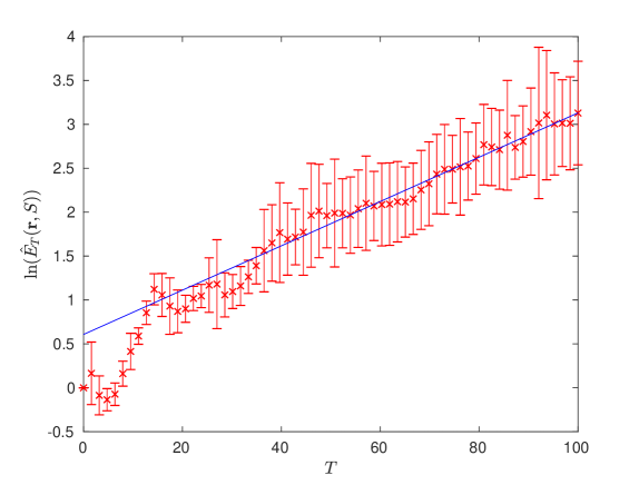
Figure 2: A simulation of the Hunt and Ott algorithm on a chaotic system with no equilibrium points.

Example 5.6.

We consider now the motion of a double pendulum consisting of two point masses $m_{1}$, $m_{2}$ joined together by two massless shafts or bars of lengths $l_{1}$, $l_{2}$. (See Figure 3.) We assume that there is no friction on the joints. If we let $\theta_{i}(t)$ to be the angle that the shaft $l_{i}$ makes with the vertical direction, $i=1,2$, then the equations for the motion of such a system are given after simplification by:

$$l_{1}\ddot{\theta}_{1}(t) = \frac{T_{2}}{m_{1}}\,\sin(\theta_{2}(t)-\theta_{1}(t))-g\sin\theta_{1}(t),$$

$$l_{2}\ddot{\theta}_{2}(t) = -\frac{T_{1}}{m_{1}}\,\sin(\theta_{2}(t)-\theta_{1}(t)),$$

where $g$ is the constant of gravity acceleration and $T_{1},T_{2}$, the tensions in the shafts, are solutions of the system

$$\left[\begin{array}[]{cc}\frac{1}{m_{1}}&-\frac{1}{m_{1}}\,\cos(\theta_{2}(t)-\theta_{1}(t))\\ -\frac{1}{m_{1}}\,\cos(\theta_{2}(t)-\theta_{1}(t))&\frac{1}{m_{1}}+\frac{1}{m_{2}}\end{array}\right]\left[\begin{array}[]{c}T_{1}\\ T_{2}\end{array}\right]=\left[\begin{array}[]{c}l_{1}\dot{\theta}_{1}^{2}(t)+g\cos\theta_{1}(t)\\ l_{2}\dot{\theta}_{2}^{2}(t)\end{array}\right].$$

Figure 3: Frictionless double pendulum.

This system is well known to be chaotic (cf. [3], [15]). The Hunt and Ott algorithm was tested in this case with $N=1000$ and $20$ samples, and restraining region

$$S=\left\{(\theta_{1},\dot{\theta}_{1},\theta_{2},\dot{\theta}_{2})\,:\,\left|\theta_{i}\right|\leq 100,\quad\left|\dot{\theta}_{i}\right|\leq 20,\quad i=1,2\right\}.$$

In Figure 4 we show the results for this simulation. The slope of approximately $5.7016$ in this picture is consistent with the chaotic character of this system.

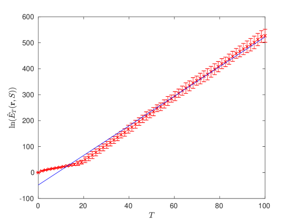
Figure 4: Simulation using the Hunt and Ott Frictionless double pendulum.

6 Numerical results

In this section we present various numerical results for the behaviour of solutions of (4.3) when the potential $\phi$ is given by (2.1). In particular, using the Hunt and Ott method, we test the system (4.3) for chaotic behaviour.

We consider the case of (2.1) in which the parameters are given by

$$c_{1}=1,\quad c_{2}=2,\quad\delta_{1}=12,\quad\delta_{2}=6.$$ (6.1)

The stability and multiplicity of the equilibrium states of (4.3) (cf. Proposition 3.1) was fully analysed in [14] for this case. We briefly review those results that are more relevant to the present discussion. In Figure 5 (reproduced from [14]) we show a projection of the bifurcation diagram of equilibrium states for the particular case (6.1). (The notation here is as in Proposition 3.1 where $a,b,c$ represent the sides of the triangular configuration of the array.) In this figure there are three bifurcation points at the following approximate values of the area parameter $A$ in (4.3): $A_{0}=0.5877$ (primary bifurcation) and $A_{1}=0.6251$, $A_{2}=0.6670$ (secondary bifurcations). The is also a turning point at $A_{-1}=0.5855$ corresponding to a trans–critical type bifurcation from $A_{0}$. The stability, multiplicity and type of the equilibrium point is summarized in Table 1. The “type” column refers as to whether the shape of triangular array is an equilateral, isosceles, or scalene triangle.

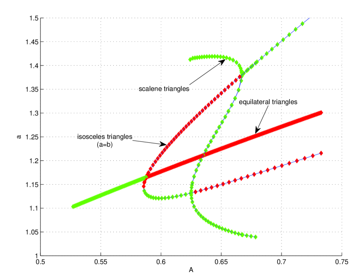
Figure 5: Bifurcation diagram for the equilibrium points of the system (4.3) for the Lennard-Jones potential (2.1) with values (6.1), green representing stable equilibria while red unstable ones.

$A$	type	stability	multiplicity
$A\in(0,A_{-1})$	equilateral	stable	one
	equilateral	stable	one
$A\in(A_{-1},A_{0})$	isosceles	stable	three
	isosceles	unstable	three
	equilateral	unstable	one
$A\in(A_{0},A_{1})$	isosceles	stable	three
	isosceles	unstable	three
	equilateral	unstable	one
$A\in(A_{1},A_{2})$	scalene	stable	six
	isosceles	unstable	six
	equilateral	unstable	one
$A\in(A_{2},\infty)$	isosceles	stable	three
	isosceles	unstable	three

Table 1: Type, stability, and multiplicity for the equilibrium points of (4.3) for the values in (6.1).

In the first simulation we examine the dynamics of the system (4.3) near the equilibrium point for the value $A=0.55$. This equilibrium point corresponds to an equilateral configuration of the array with sides $1.1270$ approximately. The corresponding equilibrium point for (4.3) is $u_{1}=0.5635$, $w_{1}=0.9760$. We introduced a perturbation of $10^{-3}$ on one of the sides of the triangular array and used the resulting values of $u_{1},w_{1}$, with velocities $v_{1},v_{2}$ both $O(10^{-4})$, as initial conditions for (4.3). In Figure 6 we show the projection onto the $u_{1}$–$w_{1}$ plane of the computed orbit of the dynamical system. Figure 7 shows the evolution of $u_{1}(t)$ and $w_{1}(t)$ as functions of time. The initial point is marked in blue and the equilibrium point in green. Both figures are consistent with a stable (not asymptotically stable) fixed point. Similar results are obtained for initial values close to other stable equilibrium corresponding to different values of $A$.

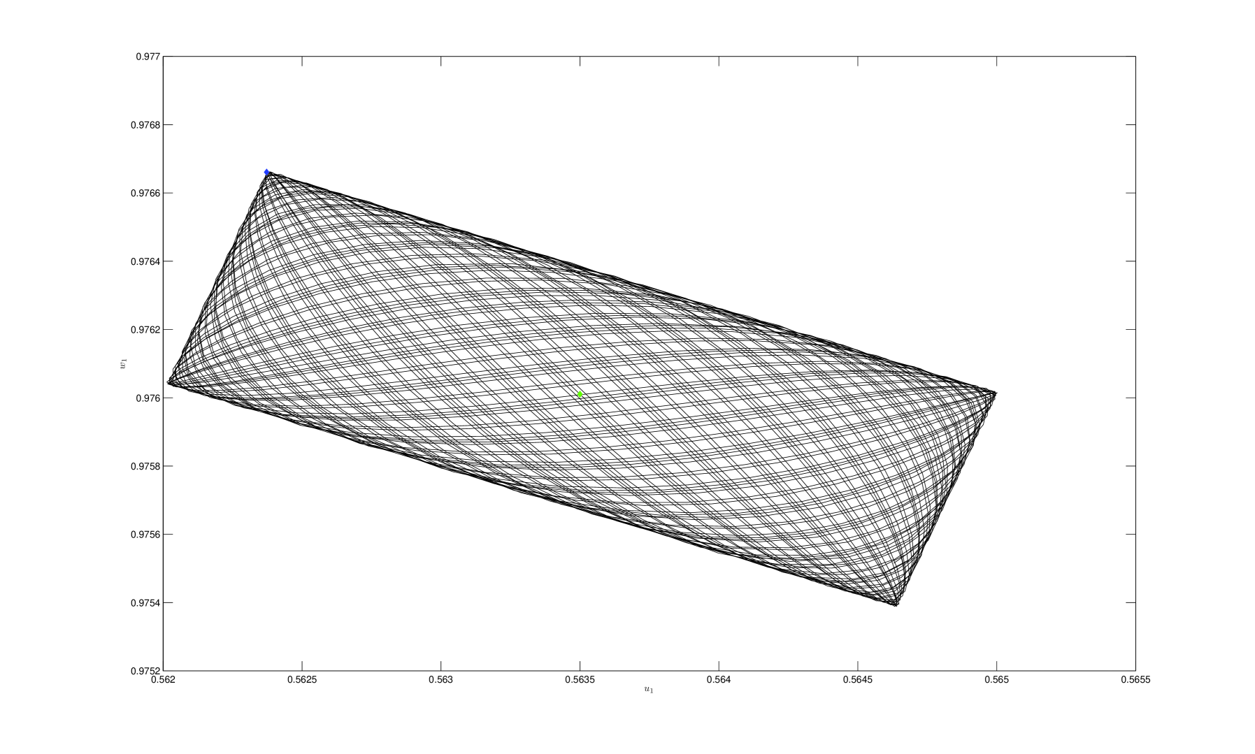
Figure 6: Sample orbit for initial point (blue) near the stable equilibrium point (green) corresponding to $A=0.55$.

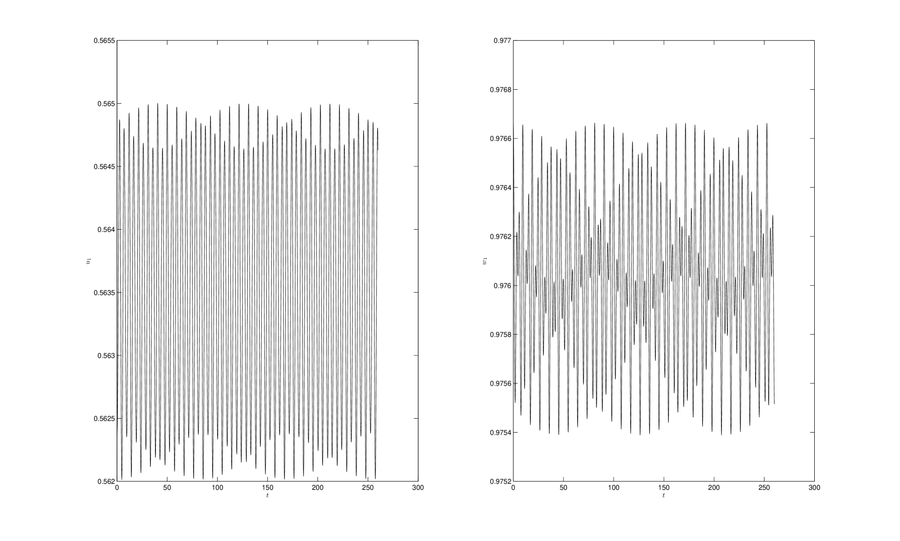
Figure 7: Graphs of $u_{1}$ and $w_{1}$ vs $t$ for the components of the orbit in Figure 6 corresponding to $A=0.55$.

We now consider the case in which $A=0.65$. According to Table 1 we have one equilateral configuration which is unstable, six isosceles unstable configurations, and six stable equilibrium points corresponding to scalene triangles. For the scalene case, the triangle sides are $1.2776,1.4182,1.0580$, the six triangular configurations obtained by permuting these numbers. In Figure 8 we show the projection onto the $u_{1}$–$w_{1}$ plane of an orbit generated with an initial point (indicated in blue) not necessarily close to any of the six stable equilibrium points (in green). Not that the orbit appears to visit “regularly” all the stable equilibrium points. In Figure 9 we show the evolution of $u_{1}(t)$ and $w_{1}(t)$ as functions of time, with the apparent random nature characteristic of a chaotic system. In Figure 10 we tested the orbit in Figure 9 for sensitivity to initial conditions. This figure was generated introducing a perturbation of $O(10^{-4})$ into the initial condition used for Figure 9. The resulting figure differs substantially from that in Figure 10, again characteristic of a chaotic system.

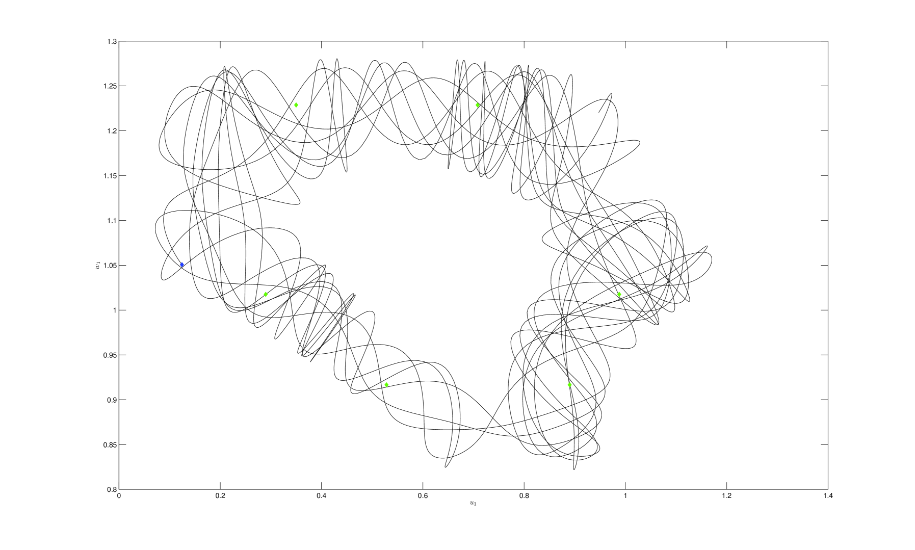
Figure 8: Sample orbit visiting all six stable equilibrium point (green) corresponding to $A=0.65$.

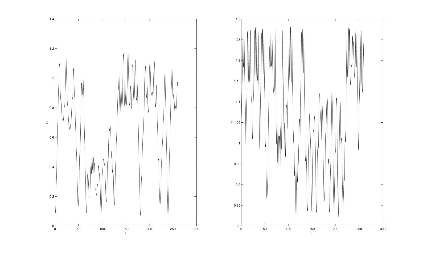
Figure 9: Graphs of $u_{1}$ and $w_{1}$ vs $t$ for the components of the orbit in Figure 8 corresponding to $A=0.65$.

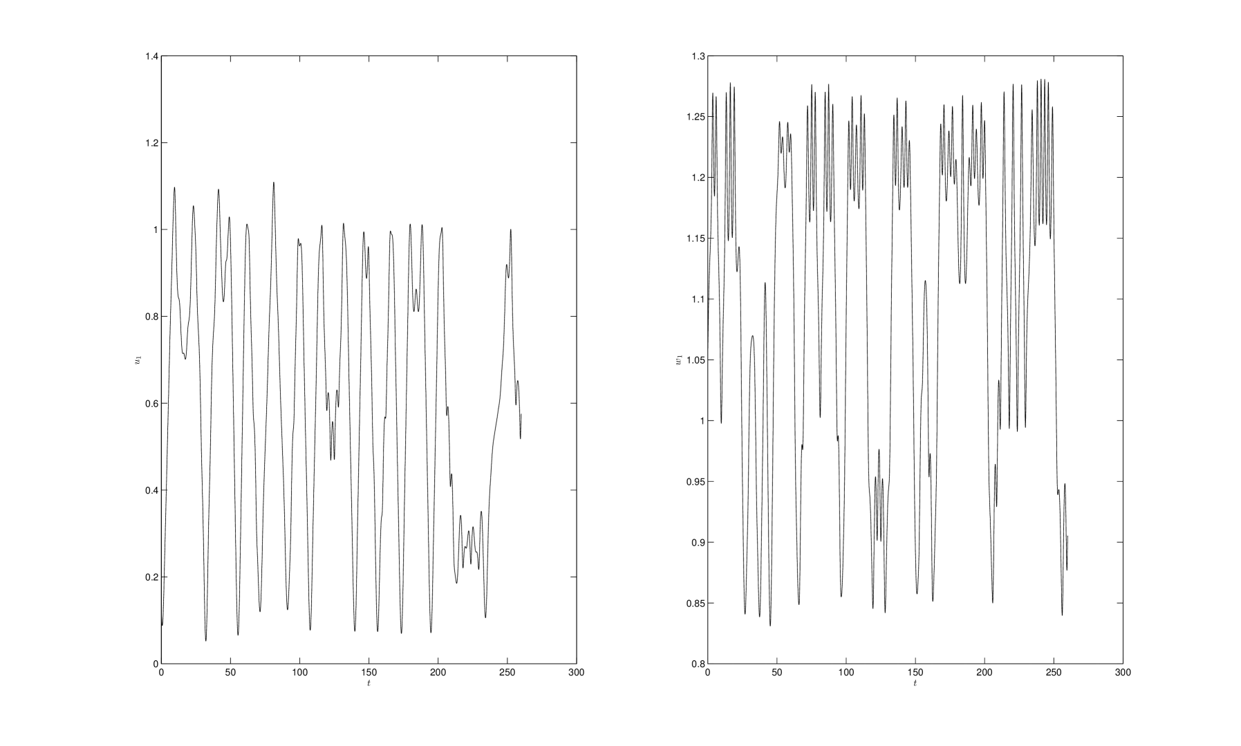
Figure 10: Graphs of $u_{1}$ and $w_{1}$ vs $t$ for the components of the orbit with initial conditions as in Figure 9 plus a perturbation $O(10^{-4})$ corresponding to $A=0.65$.

To test for possible chaotic behaviour of the system (4.3), we used the numerical scheme described at the end of Section 5 to approximate the expansion entropy $H_{0}$ for our system. Note that the entropy depends now on the area parameter $A$. As a restraining region we used:

$$S=\left\{(u_{1},w_{1},v_{1},v_{2})\,:\,-2\leq u_{1},v_{1},v_{2}\leq 2,\quad 0<w_{1}\leq 2\right\}.$$

We computed (5.7) with $N=5000$ and $50$ data samples. In Figure 11 we show a plot of the averages of the computed $\ln[\hat{E}_{T}(\mathbf{r},S)]$ for a range of values of $T$ corresponding to $A=0.65$. The red bars in the graph give intervals of plus or minus one sample standard deviation from each computed mean. As can be seen from the figure, the computed averages lie approximately on a line for large values of $T$. The slope of this line gives an approximation of $H_{0}(\mathbf{r},S)$ for our system. This slope is approximately $2.6988$ and thus according to the criteria in [10], the system (4.3) is chaotic for $A=0.65$. We performed a similar calculation for $A=0.55$. We show in Figure 12 the corresponding graph, again with the computed averages lying approximately on a line for large values of $T$, with slope of approximately $3.9548$ in this case. Thus the system is chaotic for this value of $A$ as well.

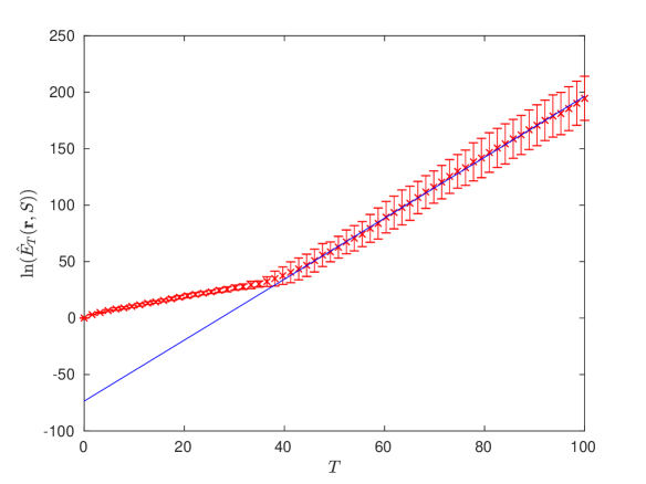
Figure 11: Graph of $\ln(\hat{E}_{T})$ vs $T$ for the system (4.3) corresponding to $A=0.65$.

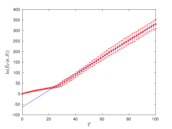
Figure 12: Graph of $\ln(\hat{E}_{T})$ vs $T$ for the system (4.3) corresponding to $A=0.55$.

7 Final comments

The criteria for chaos given by Hunt and Ott [10] leads itself to a practical numerical method for detecting chaos in dynamical systems. The method is applicable to continuous as well as to discrete dynamical systems, even non–autonomous systems. The computations can be very intensive as the method requires a large number of random points over the restraining region, and this must be repeated another number of times in order to compute the required averages. However the method is easy to run in parallel which helps to reduce the computational time.

The values of $A=0.55$ and $0.65$ are typical values for different ranges of this parameter. Thus we expect chaotic behaviour as well for values of $A$ in certain intervals. For the area parameter with value $A=0.55$, the equilibrium point of the system (4.3) is stable. If this equilibrium point is unique, then the system must have a hidden strange attractor. Examples of this type of dynamical systems are rather limited (cf. [13]). Further analysis in this direction as well as for the case $A=0.65$, and the implications of the results in this paper to the study of “cavitation” in fluids mentioned in the introduction, shall be pursued elsewhere.

Acknowledgements: This research was sponsored in part by the NSF–PREM Program of the UPRH (Grant No. DMR–1523463).

References

- [1] Bazhirov, T.T., Norman, G.E., Stegailov, V.V., Cavitation in liquid metals under negative pressures, Molecular dynamics modeling and simulation. J. Phys. Condens. Matter 2008, 20, 114113.
- [2] Blander, M., Katz, J., Bubble Nucleation in Liquids. AlChE J. 1975, 21, 833–848.
- [3] Deleanu, D., Concerning the behavior of the harmonically forced double pendulum, Universitatii Maritime Constanta, Vol. 12, Issue 16, pp. 229–236, 2011.
- [4] Fond, C., Cavitation Criterion for Rubber Materials: A Review of Void-Growth Models, J. Polym. Sci. Part B Polym. Phys., 39, 2081–2096, 2001.
- [5] Hairer, E., Geometric Integration of Ordinary Differential Equations on Manifolds, BIT Numerical Mathematics, 41, pp. 996–1007, 2001.
- [6] Hairer, E., Solving Differential Equations on Manifolds, Université de Genève, Lecture Notes, June 2011.
- [7] Hartman, P., Ordinary Differential Equations, Birkhäuser, Boston, 1982.
- [8] Hasselblatt, B. and Katok, A., A First Course in Dynamics with a Panorama of Recent Developments, Cambridge University Press, 2003.
- [9] Horgan, C.O. and Polignone, D.A., Cavitation in nonlinearly elastic solids: A review, Appl. Mech. Rev., 48, 471–485, 1995.
- [10] Hunt, B. R. and Ott, E., Defining chaos, Chaos, 25, 097618, 2015.
- [11] Jafari, S., Sprott, J., and Nazarimehr, F., Recent new examples of hidden attractors, The European Physical Journal Special Topics, 224(8):1469-1476, 2015.
- [12] Lennard–Jones, J.E., On the Determination of Molecular Fields, Proc. R. Soc. Lond. A 106 (738), 463–477, 1924.
- [13] Molaie, M., Jafari, S., Sprott, J., and Golpayegani, S., Simple chaotic flows with one stable equilibrium, International Journal of Bifurcation and Chaos, Vol. 23, No. 11, pages 1350188, 2013.
- [14] Negrón-Marrero, P. V. and López-Serrano, M., Minimal energy configurations of finite molecular arrays, Symmetry, 11, 158, 2019.
- [15] Shinbrot, T., Grebogi, C., Wisdom, J., and Yorke, J., Chaos in a double pendulum. American Journal of Physics, American Association of Physics Teachers, 60, pp.491–499, 1992.
- [16] Sprott, J., Some simple chaotic flows, Physical Review E50, pp. R647–R650, 1994.