Analysis of the Results of Metadynamics Simulations by metadynminer and metadynminer3d

Abstract

The molecular simulations solve the equation of motion of molecular systems, making 3D shapes of molecules four-dimensional by adding the time coordinate. These methods have a great potential in drug discovery because they can realistically model the structures of protein molecules targeted by drugs as well as the process of binding of a potential drug to its molecular target. However, routine application of biomolecular simulations is hampered by the very high computational costs of this method. Several methods have been developed to address this problem. One of them, metadynamics, disfavors states of the simulated system that have been already visited and thus forces the system to explore new and new states. Here we present the package metadynminer and metadynminer3d to analyze and visualize results from metadynamics, in particular those produced by a popular metadynamics package Plumed.

Introduction

Molecular simulations and their pioneers Martin Karplus, Michael Levitt, and Arieh Warshel have been awarded Nobel Prize in 2013 (Karplus, 2013). These methods, in particular the method of molecular dynamics simulation, computationally simulate the motions of atoms in a molecular system. A simulation starts from a molecular system defined by positions (Cartesian coordinates) of individual atoms. The heart of the method is in calculation of forces acting on individual atoms and their numerical integration in the spirit of Newtonian dynamics, i.e., conversion of a force vector to acceleration vector, velocity vector and, finally, to a new position of an atom. By repeating these steps, it is possible to reconstruct a record of atomic motions known as a trajectory.

Molecular simulations have a great potential in drug discovery. A molecule of drug influences (enhances or blocks) the function of some biomolecule in the patient’s body, typically a receptor, enzyme or other protein. These molecules are called drug targets. The process of design of a new drug can be significantly accelerated by knowledge of the 3D structure (Cartesian coordinates of atoms) of the target. With such knowledge, it is possible to find a "druggable" cavity in the target and a molecule that fits and favourably binds to this cavity to influence its function. Strong binding implies that the drug influences the target even in low doses, hence does not cause side effects by interacting with unwanted targets.

Experimental determination of 3D structures of proteins and other biomolecules is very expensive and laborious process. Molecular simulations can, at least in principle, replace such expensive and laborious experiments by computing. In principle, a molecular simulation starting from virtually any 3D shape of a molecule would end up in energetically the most favourable shape. This is analogous with water flowing from mountains to valleys and not in the opposite way.

Unfortunately, this approach is extremely computationally expensive. The integration step of a simulation must be small enough to comprise the fastest motions in the molecular system. In practical simulations, it is necessary to use femtosecond integration steps. This means that it is necessary to carry out thousands of steps to simulate picoseconds, millions of steps to simulate nanoseconds, and so forth. In each step, it is necessary to evaluate a substantial number of interactions between atoms. As the result of this, it is possible to routinely simulate nano- to microseconds. Longer simulations require special high-performance computing resources.

Protein folding, i.e., the transition from a quasi-random to the biologically relevant 3D structure, takes place in microseconds for very small proteins and in much longer time scales for pharmaceutically interesting proteins. For this reason, prediction of a 3D structure by molecular simulations is limited to few small and fast folding proteins. For large proteins it is currently impossible or at least far from being routine.

Several methods have been developed to address this problem. Metadynamics (Laio and Parrinello, 2002) uses artificial forces to force the system to explore states that have not been previously explored in the simulation. At the beginning of the simulation, it is necessary to chose some parameters of the system referred to as collective variables. For example, numerically expressed compactness of the protein can be used as a collective variable to accelerate its folding from a noncompact to a compact 3D structure. Metadynamics starts as a usual simulation. After a certain number of steps (typically 500), the values of the collective variables are calculated an from this moment this state becomes slightly energetically disfavored due to the addition of an artificial bias potential in the shape of a Gaussian hill. After another 500 steps, another hill is added to the bias potential and so forth. These Gaussian hills accumulate until they "flood" some energy minimum and help the system to escape this minimum and explore various other states (Figure 1). In analogy to water floating from mountains to valleys, metadynamics adds "sand" to fill valleys to make water flow from valleys back to mountains. This makes the simulation significantly more efficient compared to a conventional simulation because "water" does not get stuck anywhere.

By the application of metadynamics, it is possible to significantly accelerate the process of folding. Hopefully, by the end of metadynamics we can see folded, unfolded, and many other states of the protein. However, the interpretation of the trajectory is not straightforward. In standard molecular dynamics simulation (without metadynamics), the state which is the most populated is the most populated in reality. This is not true anymore with metadynamics. Here comes the time for metadynminer and metadynminer3d.

Metadynminer and metadynminer3d use the results of metadynamics simulations to calculate the free energy surface of the molecular system. The most favoured states (states most populated in reality) correspond to minima on the free energy surface. The state with the lowest free energy is the most populated state in the reality, i.e., the folded 3D structure of the protein.

As an example to illustrate metadynamics and our package, we use an ultrasimple molecule of "alanine dipeptide" (Figure 1). This molecule can be viewed as a "protein" with just one amino acid residue (real proteins have hundreds or thousands of amino acid residues). As a collective variable it is possible to use an angle $\phi$ defined by four atoms. Biasing of this collective variable accelerates a slow rotation around the corresponding bond. Figure 1 shows the free energy surface of alanine dipeptide as the black thick line. It is not known before the simulation. The simulation starts from the state B. After 500 simulation steps, the hill is added (the hill is depicted as the red line, the flooding potential ("sand") at the top, the free energy surface with added flooding potential at the bottom). Sum of 10, 100, 200, 500, and 700 hills is depicted as yellow to blue lines.

At the end of simulation the free energy surface is relatively well flattened (blue line in Fig. 1 bottom). Therefore, the free energy surface can be estimated as a negative imprint of added "sand":

$$G(s)=-kT\log(P(s))=-V(s)=\sum_{i}w_{i}\exp(-(s-S_{i})^{2}/{2\sigma^{2}})$$ (1)

where $G$, $V$, and $P$ are free energy, metadynamics bias (flooding) potential, and probability, respectively, of a state with a collective variable $s$, $k$ is Boltzmann constant, $T$ is temperature in Kelvins, $w_{i}$ is height, $S_{i}$ is position and $\sigma_{i}$ is width of each hill. The equation can be easily generalized for two or more CVs.

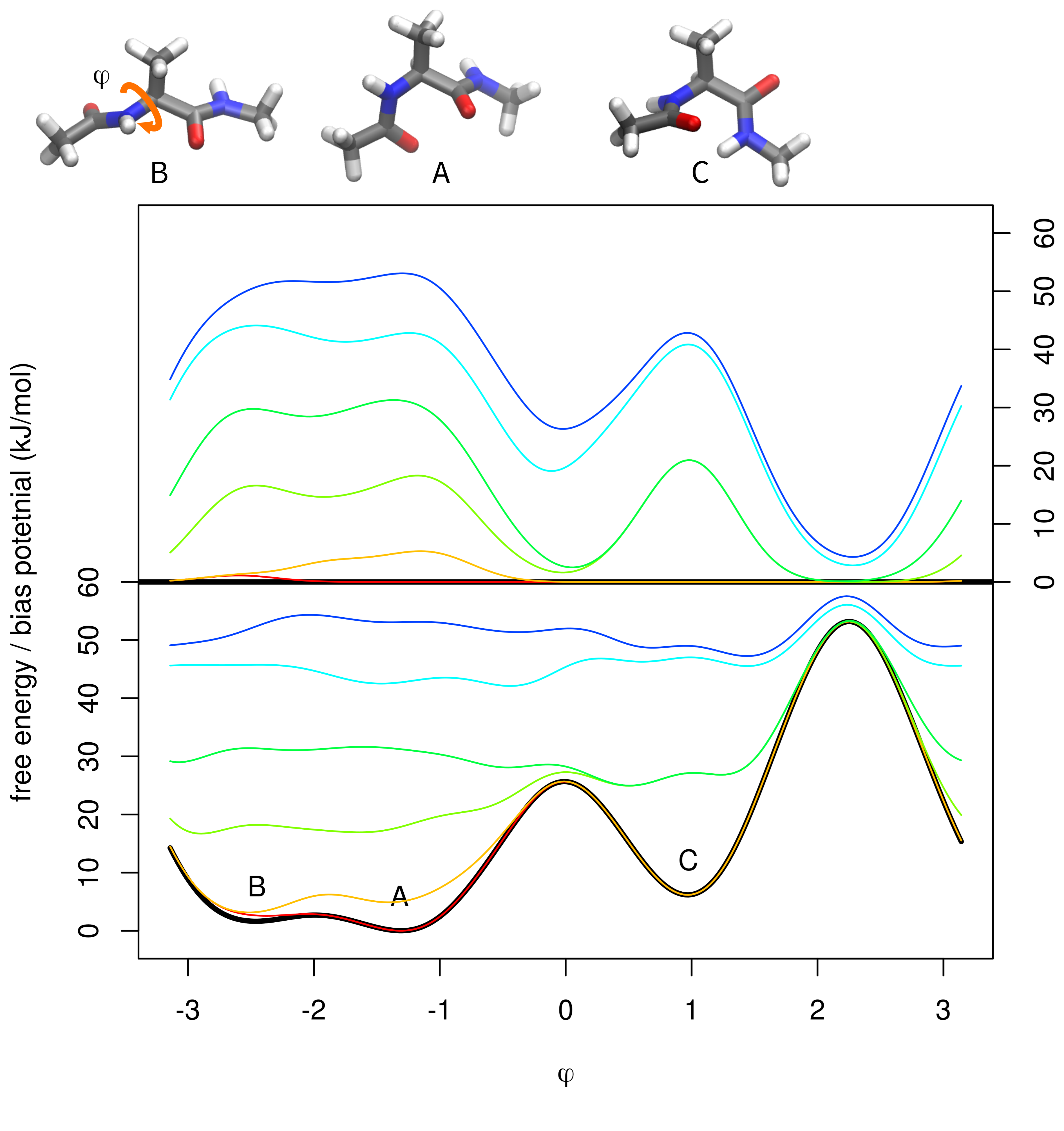
Figure 1: Metadynamics simulation of alanine dipeptide. Dihedral angle $\phi$ was used as the collective variable. The top part shows molecular structures of three free energy minima (stable structures) differing in the value of $\phi$. According to metadynamics prediction, A is the global minimum (free energy 0 kJ/mol) and B and C are local minima (1.5 and 6.3 kJ/mol, respectively). According to Equation 1, this corresponds to probabilities 0.61, 0.34, and 0.05 for A, B, and C, respectively. The middle part shows the bias potential (scaled by $(T+\Delta T)/\Delta T$) after addition of 1, 10, 100, 200, 500, and 700 hills (colors from red to blue). The bottom part shows the accurate free energy surface calculated by metadynamics with 30,000 hills (black) flooded by 1, 10, 100, 200, 500, and 700 hills (colors from red to blue). The figure was generated by metadynminer except for molecular structures and final assembly.

The original version of metadynamics was developed with constant heights of Gaussian hills. Later, a so-called well-tempered metadynamics was developed (Barducci et al., 2007), which uses decreasing hill heights to improve the accuracy of the results. This requires modification of the equation:

$$G(s)=-kT\log(P(s))=-\frac{T+\Delta T}{\Delta T}V(s)=-\frac{T+\Delta T}{\Delta T}\sum_{i}w_{i}\exp(-(s-S_{i})^{2}/{2\sigma^{2}})$$ (2)

where $\Delta T$ an input parameter with the dimension of temperature (zero for unbiased simulation and infinity for the original metadynamics with constant hill heights). Nowadays, the vast majority of metadynamics applications use the well-tempered metadynamics algorithm for its better convergence towards accurate free energy surface prediction.

There are numerous packages for molecular simulations such as Amber (Weiner and Kollman, 1981), Gromacs (Abraham et al., 2015), Gromos (Christen et al., 2005), NAMD (Phillips et al., 2020), CHARMM (Brooks et al., 2009), Acemd (Harvey et al., 2009), and others. These packages are primarily developed for basic unbiased simulations with no or very limited support of metadynamics. Plumed software (Tribello et al., 2014) has been developed to introduce metadynamics into various simulation programs. Since its introduction, Plumed articles have been cited in more than thousand papers from drug design, molecular biology, material sciences, and other fields. The R package metadynminer was developed for analysis and visualization of the results from Plumed. With a simple file conversion script, it can be used also with other simulation programs that support metadynamics.

Example of usage

Metadynminer will be presented on a bias potential from a 30 ns (30,000 hills) simulation of alanine dipeptide (Figure 1). Two rotatable bonds of the molecule, referred to as $\phi$ and $\psi$, were used as collective variables. This is basically an expansion of the free energy surface in Figure 1 to two dimensions. Hills from simulations with two collective variables ($\phi$ and $\psi$) and with one collective variable ($\phi$) are provided in metadynminer as acealanme and acealanme1d, respectively. Metadynminer3d was developed for analysis of metadynamics with three collective variables. It contains a sample data acealanmed3, with collective variables $\phi$, $\psi$ and $\omega$. We decided to distribute metadynminer and metadynminer3d separately, because of the use of different visualization tools and to keep the size of packages low. Metadynamics simulations with 1-3 CVs comprise almost all metadynamics applications nowadays (not considering special metadynamics variants).

Hills file generated by Plumed package (filename "HILLS") can be loaded to R by the function read.hills:

  hillsfile <- read.hills("HILLS", per=c(T, T))The parameter per indicates periodicity of the collective variable (dihedral angles are periodic, i.e., $+\pi\simeq-\pi$).

Typing the name hillsfile will return its dimensionality (the number of CVs) and the number of hills. A hills object can be easily plotted:

  plot(hillsfile, xlab="phi", ylab="psi")For metadynamics with one collective variable, it plots its evolution. For metadynamics with two or three collective variables, it plots a scatter plot of collective variables number 1 vs. 2 or 1 vs. 2 vs. 3, respectively (Figure 2).

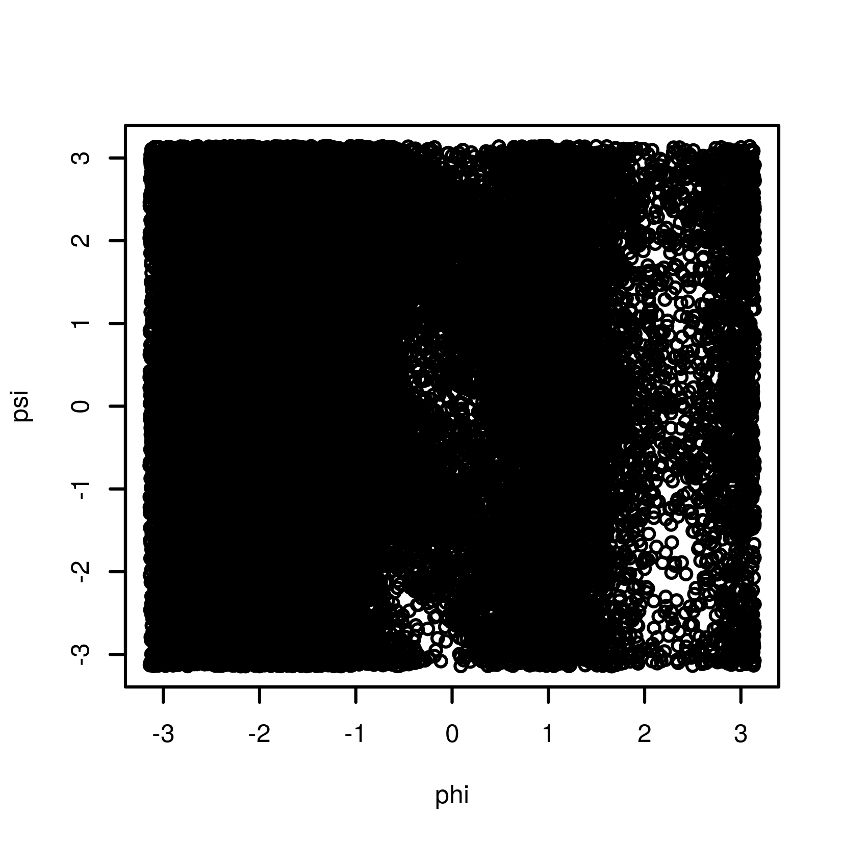
Figure 2: Scatter plot of hills position.

In well-tempered metadynamics it may be interesting to see the evolution of hill heights ($w_{i}$ in Equation 2). This can be plotted (Figure 3) by typing:

  plotheights(hillsfile)

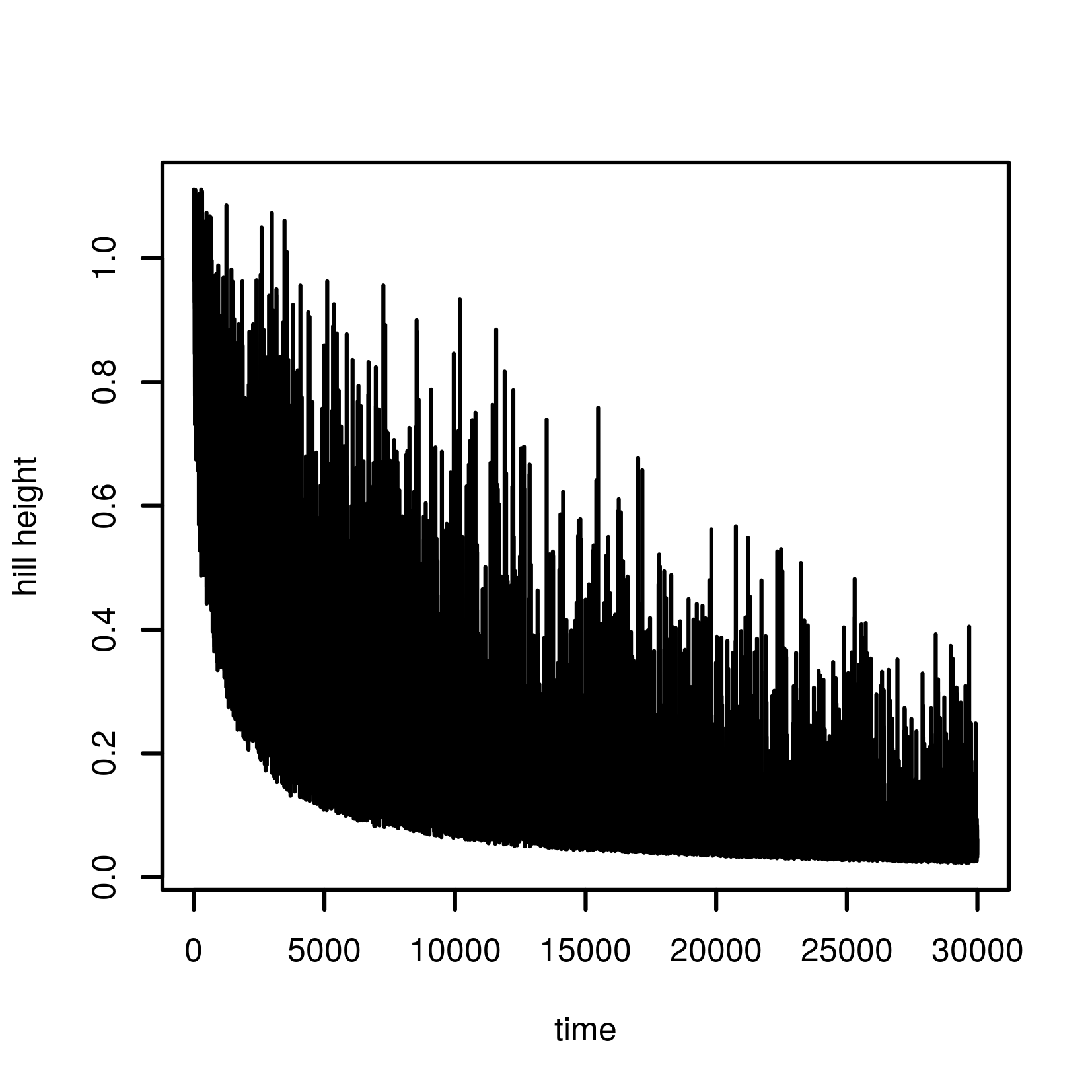
Figure 3: Evolution of heights of hills in metadynamics plotted by function plotheights.

Addition operation is available for hillsfile object. For example, multiple hills files can be concatenated.

Next, the user can sum negative values of all hills to make the free energy surface estimate by typing:

  fesurface <- fes(hillsfile)Hills files from well-tempered metadynamics are prescaled by $(\Delta T+T)/\Delta T$ when printed by Plumed, so no special action is required in metadynminer. The function fes uses the Bias Sum algorithm (Hošek and Spiwok, 2016). This function is fast because instead of evaluation of Gaussian function for every hill, it uses a precomputed Gaussian hill that is relocated to hill centers. It is also fast because it was implemented in C++ via Rcpp. Because of approximations used in the function fes, this function should be used for visualization purposes. For detailed analysis of a free energy surface, we advice to use a slow but accurate fes2 function. This function explicitly evaluates Gaussian function for every hill. It can be also used for (rarely used) metadynamics with variable hill widths.

Typing the name of the variable with a free energy surface returns its dimensionality, number of points, and free energy maximum and minimum. The same is returned by summary function. It is possible to add and subtract two free energy surfaces with the same number of grid points. The functions min and max can be used as well to calculate minimum or maximum. It is also possible to multiply or divide the free energy surface by a constant (for example, to convert kJ to kcal and vice versa). Free energy surface can be plotted (Figure 4) by typing:

  plot(fesurface, xlab="phi", ylab="psi")

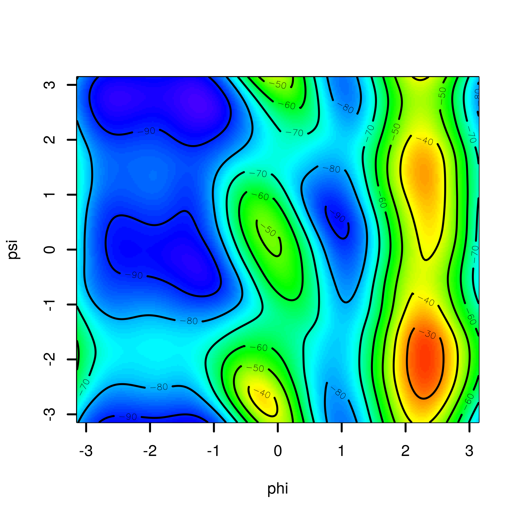
Figure 4: Free energy surface.

In metadynamics simulation, it is important to find free energy minima. The global minimum refers to the most favored state of the system (i.e., the state with the highest probability). Other local minima correspond to metastable states. The user can find free energy minima by typing:

  minima <- fesminima(fesurface)This function locates minima using a simple algorithm. The free energy surface is separated into 8, 8x8, or 8x8x8 bins (for 1D, 2D, or 3D surface, respectively). A minimum in each bin is located. Next, the program tests whether a minimum is a local minimum of the whole free energy surface. The number of grid points can be changed by ngrid parameter. Typing the name of the minima variable will return the table of minima (denoted as A, B, C, … in the order of their free energies), their collective variables, and free energy values.

In addition, the function summary provides populations of each minimum calculated as:

$$P_{i,rel}=\exp(-G_{i}/kT)$$ (3)

$$P_{i}=P_{i,rel}/\sum(P_{j,rel})$$ (4)

  letter CV1bin CV2bin        CV1        CV2 free_energy relative_pop
1      A     78    236 -1.2443171  2.6487938   -97.26095 8.614856e+16
2      B     28    240 -2.4763142  2.7473536   -95.63038 4.480527e+16
3      C     74    118 -1.3428769 -0.2587194   -94.73163 3.124915e+16
4      D    166    151  0.9239978  0.5543987   -91.66626 9.143024e+15
5      E    170    251  1.0225576  3.0183929   -84.37799 4.920882e+14
         pop
1 50.1335658
2 26.0741201
3 18.1852268
4  5.3207200
5  0.2863674

Plot function on a fesminima output provides the same plot as for fes output with additional letters indicating minima (Figure 5).

Figure 5: Free energy surface with indicated free energy minima A-E.

It is essential to evaluate the accuracy of metadynamics and to decide when the simulation is accurate enough so that it can be stopped. For this purpose, it is useful to look at the evolution of relative free energies. The relative free energies (for example, the free energy difference of minima A and C) evolve rapidly at the beginning of the simulation, and with the progress of the simulation, their difference is converging towards the real free energy difference. Function feprof calculates the evolution of free energy differences from the global minimum (global at the end of the simulation). It can be used as:

  prof<-feprof(minima)Function summary provides minima and maxima of these free energy differences. The evolution can be plotted (Figure 6) by typing:

  plot(prof)

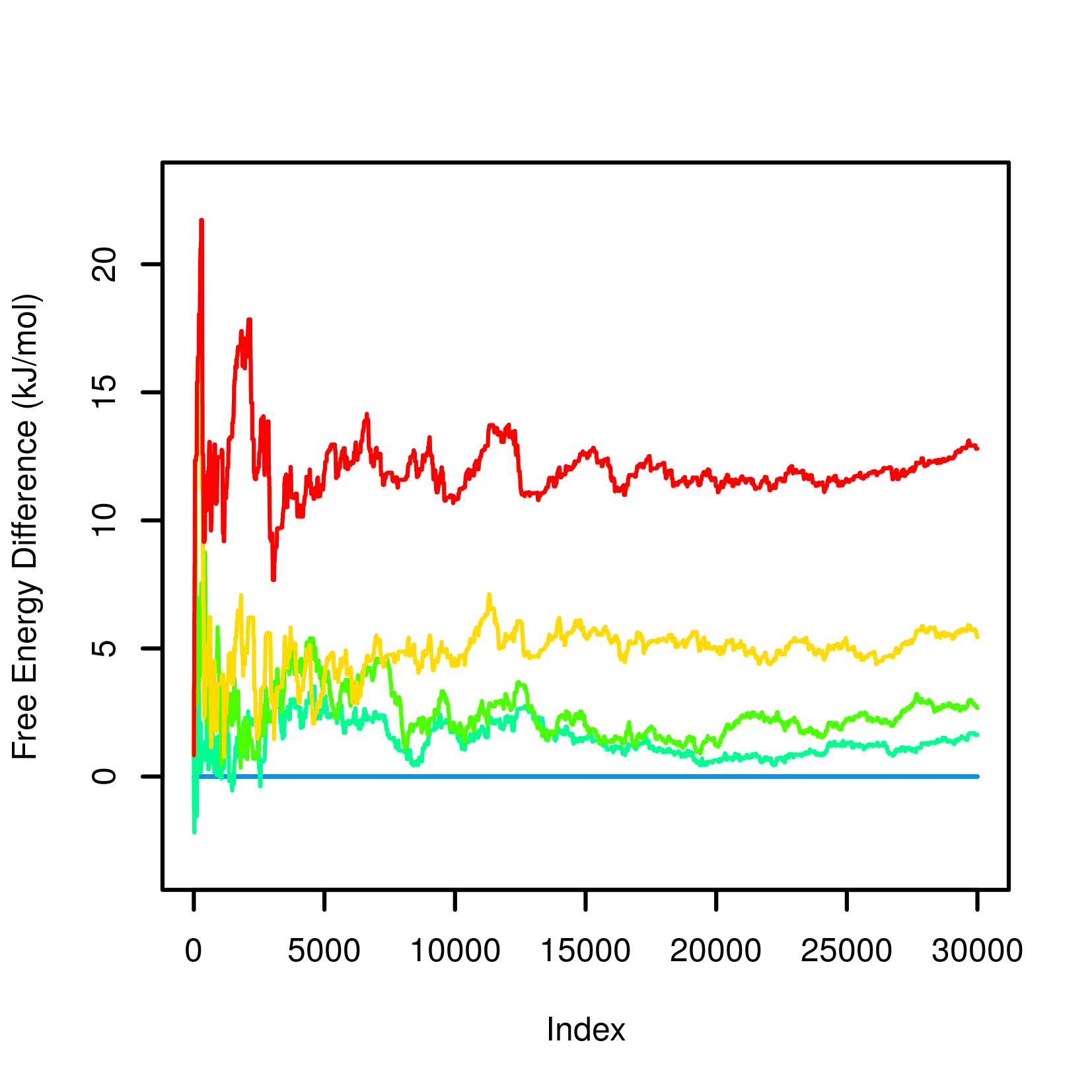
Figure 6: Evolution of free energy differences.

Beside minima, another important points on the free energy surface are transition states. Change of the molecular structure from one minimum to another takes place via a path with the lowest energy demand. The state with the highest energy along this path is called the transition state. Free energy difference between the initial and transition state can be used to predict kinetics (rates) of the studied molecular process. Furthermore, identification of transition states is important in drug design because compounds designed to mimic a transition states of an enzymatic reaction are often potent enzymes inhibitors and drugs (Itzstein et al., 1993).

In metadynminer, such path can be identified by Nudged Elastic Band method (Henkelman and Jónsson, 2000). Briefly, this method plots a line between selected minima as an initial approximation of the transition path. Next, this line is curved so that the corresponding physical process becomes feasible. This function can be applied on, for example, minima A and D as:

  nebAD<-neb(minima, min1="A", min2="D")The result can be analyzed by summary (to provide kinetics of the A to D and D to A change predicted by Eyring equation (Eyring, 1935)), by plot (to plot the free energy profile of the molecular process) and by pointsonfes of linesonfes (to plot the path on top of the free energy surface). The last example can be invoked by:

  plot(minima, xlab="phi", ylab="psi")  linesonfes(nebAD, lwd=4)The resulting plot is depicted in Figure 7

Figure 7: Path of transition from A to D projected onto free energy surface.

Let us also briefly present metadynminer3d. This package uses packages rgl and misc3d to plot the free energy surface as an interactive (mouse rotatable) isosurface in the space of three collective variables (see Figure 8). Metadynminer3d can produce interactive WebGL visualizations using writeWebGL command from the rgl package.

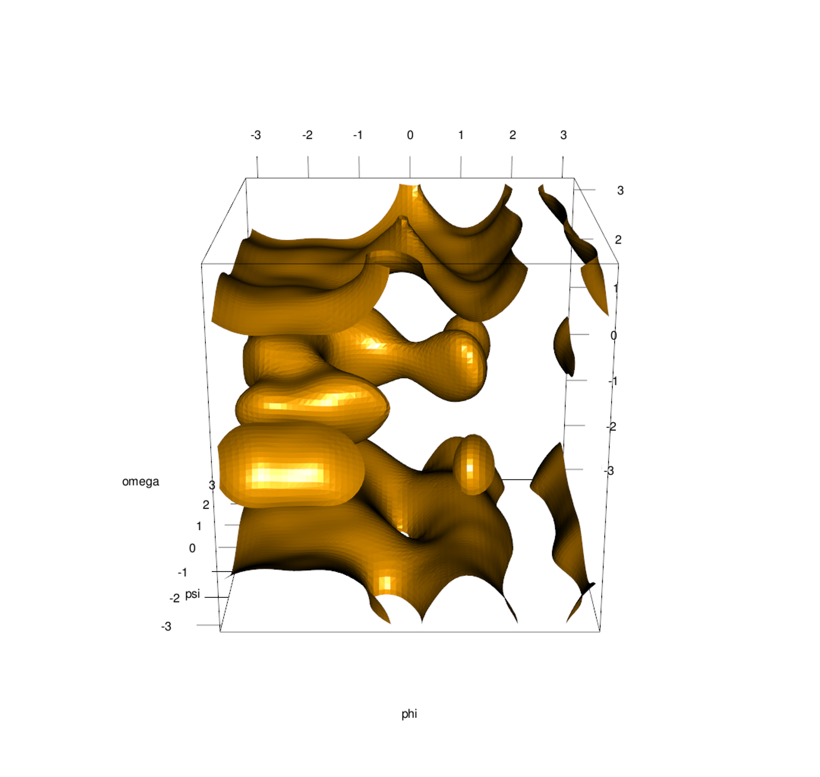
Figure 8: 3D free energy surface depicted as isosurface at $-30$ kJ/mol.

Metadynminer and metadynminer3d were developed to be highly flexible. This flexibility can be demonstrated on two examples. First, it is useful to visualize the progress of metadynamics as a video sequence showing the evolution of the free energy surface. The code to generate corresponding images can be written in metadynminer as:

tfes<-fes(acealanme, tmax=100)png("snap%04d.png")plot(acealanme, zlim=c(-200,0))for(i in 1:299) {  tfes<-tfes+fes(acealanme, imin=100*i+1, imax=100*(i+1))  plot(tfes, zlim=c(-200,0), xlab="phi", ylab="psi")}dev.off()This generates a series of images that can be concatenated by external software to make a video file.

The second example demonstrates a more complicated analysis of the results from metadynamics. Functions fes and fes2 use equations 1 and 2 to predict the free energy surface. A limitation of this approach is that the prediction of the free energy surface is based only on the positions of hills. The evolution of collective variables between hills depositions is not used. As an alternative, it is possible to use reweighting (Torrie and Valleau, 1977; Tiwary and Parrinello, 2015). This approach calculates the free energy surface from hills positions as well as from evolution of collective variables. Briefly, regions of the free energy surface that are sampled despite being disfavored by high flooding potential have higher weights than those disfavored by low flooding potential. This approach is in general more accurate. Reweighting can be done using the code:

bf <- 15
kT <- 8.314*300/1000
npoints <- 50
maxfes <- 75
outfes <- 0*fes(acealanme, npoints=npoints)
s1 <- c()
s2 <- c()
for(i in 1:50) {
  step <- i*length(acealanme$time)/50
  cfes <- fes(acealanme, imax=step)
  s1 <- c(s1, sum(exp(-cfes$fes/kT)))
  s2 <- c(s2, sum(exp(-cfes$fes/kT/bf)))
}
ebetac <- s1/s2
cvs <- read.table("COLVAR")
nsamples <- nrow(cvs)
xlim <- c(-pi,pi)
ylim <- c(-pi,pi)
for(i in 1:nsamples) {
  step <- (i-1)*50/nsamples+1
  ix <- npoints*(cvs[i,2]-xlim[1])/(xlim[2]-xlim[1])+1
  iy <- npoints*(cvs[i,3]-ylim[1])/(ylim[2]-ylim[1])+1
  outfes$fes[ix,iy] <- outfes$fes[ix,iy] + exp(cvs[i,4]/kT)/ebetac[step]
}
outfes$fes[!outfes$fes>0] <- maxfes
outfes$fes <- -kT*log(outfes$fes)
plot(outfes, xlab="phi", ylab="psi")

where bf is the bias factor ($(T+\Delta T)/T$ in Equation 2), kT is temperature in Kelvins multiplied by Boltzmann constant, npoints is the granularity of the resulting free energy surface and maxfes is the maximal possible free energy (to avoid problems with infinite free energy in unsampled regions). First, outfes is introduced as a zero free energy surface. The first loop calculates the correction ebetac for the evolution of flooding potential developed by Tiwary and Parrinello (Tiwary and Parrinello, 2015). Next, a file with the evolution of collective variables COLVAR (from the same simulation used to generate acealanme dataset, available at https://www.metadynamics.cz/metadynminer/data/) is read. The second loop evaluates the sampling weighted by the factor $\exp(V(s)/kT)$ divided by ebetac to correct for the evolution of the bias potential (Tiwary and Parrinello, 2015). Finally, probabilities are converted to the free energy surface and plotted (Figure 9).

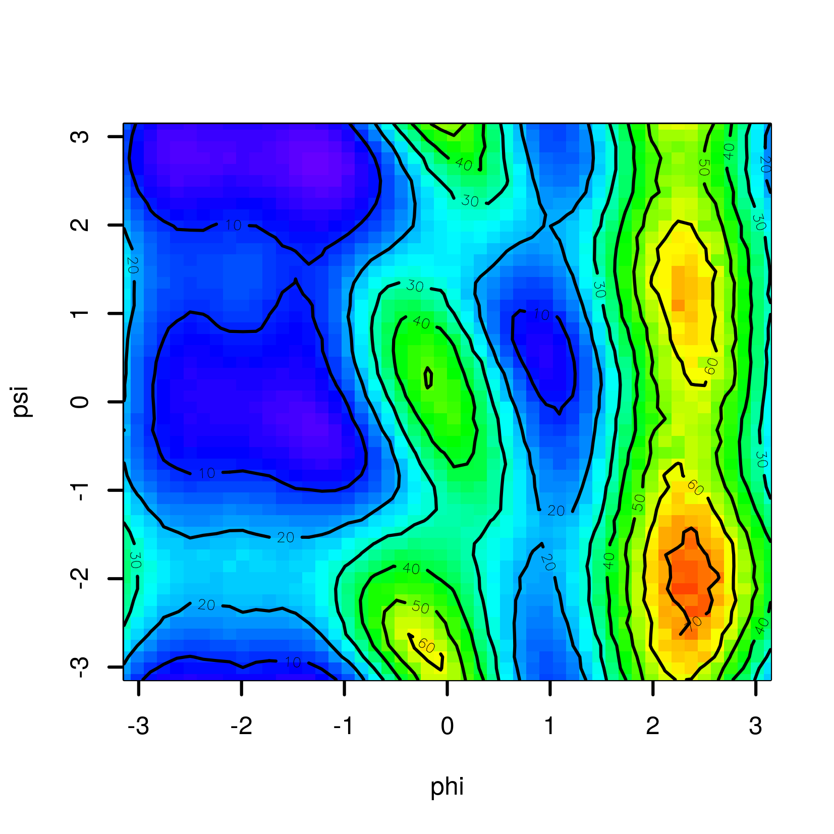
Figure 9: Free energy surface calculated by reweighting by Tiwary and Parrinello (2015).

Simulation details

All simulations were done using Gromacs 2016.4 (Abraham et al., 2015) patched by Plumed 2.4b (Tribello et al., 2014). Alanine dipeptide was modeled using Amber99SB-ILDN force field (Lindorff-Larsen et al., 2010). The simulated system contained alanine dipeptide and 874 TIP3P (Jorgensen et al., 1983) water molecules. The temperature was kept constant at 300 K using Bussi thermostat (Bussi et al., 2007). Metadynamics hills of height 1 kJ/mol (bias factor 10) and widths 0.3 rad were added every 1 ps. Two simulations were done, one with one dihedral angle $\phi$ (dataset acealanme1d), two dihedral angles $\phi$ and $\psi$ (dataset acealanme), or with three angle $\phi$, $\phi$ and $\omega$ (dataset acealanme3d in metadynminer3d). Supporting material is available at https://www.metadynamics.cz/metadynminer/data/ or in Plumed nest (PLUMED consortium, 2019) at https://www.plumed-nest.org/eggs/20/023/.

Summary

The package metadynminer and metadynminer3d provides fast algorithm Bias Sum (Hošek and Spiwok, 2016) for calculation of free energy surfaces from metadynamics. This algorithm is available in our on-line tool MetadynView (http://metadyn.vscht.cz), but this tools is intended for routine checking of the progress of metadynamics simulations rather than for in deep analysis and visualization. Besides this, users of metadynamics use built-in functions in Plumed or various in-lab scripts. Such scripts do not provide appropriate flexibility in analysis and visualization.

We see the biggest advantage in the fact that metadynminer can produce publication quality figures via graphics output functions in R. As shown above, using a simple for loop it is possible to plot individual snapshots and concatenate them outside R to make a movie. Metadynminer3d provides the possibility to produce interactive 3D web models by WebGL technology. We also tested 3D printing of a free energy surface that is very easy using metadynminer and rayshader. Various tips and tricks can be found on the website of the project (https://www.metadynamics.cz/metadynminer/).

Another advantage we see in reporting of results. Reproducibility is a big issue in science, including molecular simulations. Packages like knitr or rmarkdown ca be used to record all steps of data analysis pipeline to compile a report for routine and reproducible use of metadynamics.

Dalibor Trapl
Department of Biochemistry and Microbiology, University of Chemistry and Technology, Prague
Technicka 3, Prague 6, 166 28
Czech Republic
ORCID: 0000-0002-3435-5841
traplda@vscht.cz

Vojtech Spiwok
Department of Biochemistry and Microbiology, University of Chemistry and Technology, Prague
Technicka 3, Prague 6, 166 28
Czech Republic
ORCID: 0000-0001-8108-2033
spiwokv@vscht.cz

References

- Abraham et al. (2015) J. M. Abraham, T. Murtola, R. Schulz, S. Páll, J. C. Smith, B. Hess, and L. Erik. Gromacs: High performance molecular simulations through multi-level parallelism from laptops to supercomputers. SoftwareX, 1–2:19–25, 2015. URL https://doi.org/10.1016/j.softx.2015.06.001.
- Barducci et al. (2007) A. Barducci, G. Bussi, and M. Parrinello. Well-tempered metadynamics: A smoothly converging and tunable free-energy method. Physical Review Letters, 100(2):020603, 2007. URL https://doi.org/10.1103/PhysRevLett.100.020603.
- Brooks et al. (2009) B. R. Brooks, C. L. Brooks, A. D. Mackerell, L. Nilsson, R. J. Petrella, B. Roux, Y. Won, G. Archontis, C. Bartels, S. Boresch, A. Caflisch, L. Caves, Q. Cui, A. R. Dinner, M. Feig, S. Fischer, J. Gao, M. Hodoscek, W. Im, K. Kuczera, T. Lazaridis, J. Ma, V. Ovchinnikov, E. Paci, R. W. Pastor, C. B. Post, J. Z. Pu, M. Schaefer, B. Tidor, R. M. Venable, H. L. Woodcock, X. Wu, W. Yang, D. M. York, and M. Karplus. Charmm: The biomolecular simulation program. Journal of Computational Chemistry, 30(10):1545–1614, 2009. URL https://doi.org/10.1002/jcc.21287.
- Bussi et al. (2007) G. Bussi, D. Donadio, and M. Parrinello. Canonical sampling through velocity rescaling. Journal of Chemical Physics, 1(126):014101, 2007. URL https://doi.org/10.1063/1.2408420.
- Christen et al. (2005) M. Christen, P. H. Hünenberger, D. Bakowies, R. Baron, R. Bürgi, D. P. Geerke, T. N. Heinz, M. A. Kastenholz, V. Kräutler, C. Oostenbrink, C. Peter, D. Trzesniak, and W. F. van Gunsteren. The gromos software for biomolecular simulation: Gromos05. Journal of Computational Chemistry, 26(16):1719–1751, 2005. URL https://doi.org/10.1002/jcc.20303.
- Eyring (1935) H. Eyring. The activated complex in chemical reactions. The Journal of Chemical Physics, 3(2), 1935. URL https://doi.org/10.1063/1.1749604.
- Harvey et al. (2009) M. J. Harvey, G. Giupponi, and G. D. Fabritiis. Acemd: Accelerating biomolecular dynamics in the microsecond time scale. Journal of Chemical Theory and Computation, 5(6):1632–1639, 2009. URL https://doi.org/10.1021/ct9000685.
- Henkelman and Jónsson (2000) G. Henkelman and H. Jónsson. Improved tangent estimate in the nudged elastic band method for finding minimum energy paths and saddle points. The Journal of Chemical Physics, 113(22):9978–9985, 2000. URL https://doi.org/10.1063/1.1323224.
- Hošek and Spiwok (2016) P. Hošek and V. Spiwok. Metadyn view: Fast web-based viewer of free energy surfaces calculated, by metadynamics. Computer Physics Communications, 198:222–229, 2016. URL https://doi.org/10.1016/j.cpc.2015.08.037.
- Itzstein et al. (1993) M. v. Itzstein, W.-Y. Wu, G. B. Kok, M. S. Pegg, J. C. Dyasson, B. Jin, T. V. Phan, M. L. Smythe, H. F. White, S. W. Oliver, P. M. Colman, J. N. Varghese, D. M. Ryan, J. M. Woods, R. C. Bathell, V. J. Hotham, J. M. Cameron, and C. R. Penn. Rational design of potent sialidase-based inhibitors of influenza virus replication. Nature, 363:418–423, 1993. URL https://doi.org/10.1038/363418a0.
- Jorgensen et al. (1983) W. L. Jorgensen, J. Chandrasekhar, J. D. Madura, R. W. Impey, and M. L. Klein. Comparison of simple potential functions for simulating liquid water. The Journal of Chemical Physics, 79(2):926, 1983. URL https://doi.org/10.1063/1.445869.
- Karplus (2013) M. Karplus. Nobel lecture, 2013. URL https://www.nobelprize.org/prizes/chemistry/2013/karplus/lecture/.
- Laio and Parrinello (2002) A. Laio and M. Parrinello. Escaping free-energy minima. Proceedings of the National Academy of Sciences of the United States of America, 20(99):12562–12566, 2002. URL https://doi.org/10.1073/pnas.202427399.
- Lindorff-Larsen et al. (2010) K. Lindorff-Larsen, S. Piana, K. Palmo, P. Maragakis, J. L. Klepeis, R. O. Dror, and D. E. Shaw. Improved side-chain torsion potentials for the amber ff99sb protein force field. Proteins: Structure, Function, and Bioinformatics, 78(8):1950–1958, 2010. URL https://doi.org/10.1002/prot.22711.
- Phillips et al. (2020) J. C. Phillips, D. J. Hardy, J. D. C. Maia, J. E. Stone, J. V. Ribeiro, R. C. Bernardi, R. Buch, G. Fiorin, J. Hénin, W. Jiang, R. McGreevy, M. C. R. Melo, B. K. Radak, R. D. Skeel, A. Singharoy, Y. Wang, B. Roux, A. Aksimentiev, Z. Luthey-Schulten, L. V. Kalé, K. Schulten, C. Chipot, and E. Tajkhorshid. Scalable molecular dynamics on cpu and gpu architectures with namd. Journal of Chemical Physics, 153(4):044130, 2020. URL https://doi.org/10.1063/5.0014475.
- PLUMED consortium (2019) PLUMED consortium. Promoting transparency and reproducibility in enhanced molecular simulations. Nature Methods, 16:670–673, 2019. URL https://doi.org/10.1038/s41592-019-0506-8.
- Tiwary and Parrinello (2015) P. Tiwary and M. Parrinello. A time-independent free energy estimator for metadynamics. The Journal of Physical Chemistry B, 119(3):736–742, 2015. URL https://doi.org/10.1021/jp504920s.
- Torrie and Valleau (1977) G. M. Torrie and J. P. Valleau. Nonphysical sampling distributions in monte carlo free-energy estimation: Umbrella sampling. Journal of Computational Physics, 23:187–199, 1977. URL https://doi.org/10.1016/0021-9991(77)90121-8.
- Tribello et al. (2014) G. A. Tribello, M. Bonomi, D. Branduardi, C. Camilloni, and G. Bussi. Plumed 2: New feathers for an old bird. Computer Physics Communications, 185(2):604–613, 2014. URL https://doi.org/10.1016/j.cpc.2013.09.018.
- Weiner and Kollman (1981) P. K. Weiner and P. A. Kollman. Amber: Assisted model building with energy refinement. a general program for modeling molecules and their interactions. Journal of Computational Chemistry, 2(3):287–303, 1981. URL https://doi.org/10.1002/jcc.540020311.