Electron-capture decay in isotopic transfermium chains from self-consistent calculations

Abstract

Weak decays in heavy nuclei with charge numbers $Z=101-109$ are studied within a microscopic formalism based on deformed self-consistent Skyrme Hartree-Fock mean-field calculations with pairing correlations. The half-lives of $\beta^{+}$ decay and electron capture are compared with $\alpha$-decay half-lives obtained from phenomenological formulas. Transfermium isotopes of Md, No, Lr, Rf, Db, Sg, Bh, Hs, and Mt that can be produced in the frontier of cold and hot fusion-evaporation channels are considered. Several isotopes are identified whose $\beta^{+}/EC$- and $\alpha$-decay half-lives are comparable. The competition between these decay modes opens the possibility of new pathways towards the islands of stability.

I Introduction

Understanding superheavy nuclei (SHN) is a topical issue that attracts a great deal of research activity. The synthesis of new SHN is a long story that has already led in the last decades to the discovery of a large number of new elements (see hofmann_00 ; oganessian_07 ; hamilton_13 ; oganessian_15 ; oganessian_15_npa ; hofmann_16 ; giuliani_19 for a review).

Cold-fusion reactions were first used to synthesize SHN with $Z=107-113$ by using target nuclei ²⁰⁸Pb and ²⁰⁹Bi and medium-mass stable isotopes of Ti, Cr, Fe, Ni, and Zn as projectiles hofmann_00 ; hamilton_13 ; morita_04 . In these cold reactions the compound nucleus produced has relatively low excitation energy and typically evaporates one or two neutrons. Attempts to produce heavier nuclei with these type of reactions failed because of the fast decreasing of the production cross sections for increasing charge of the projectiles. This difficulty was solved by using more asymmetric reactions with both target and projectile having a large neutron excess and thus, decreasing the Coulomb repulsion. In practice, these hot-fusion reactions were carried out with long-lived actinide nuclei from ²³⁸U to²⁴⁹Cf as targets and the double magic nucleus ⁴⁸Ca as projectiles. The method was successfully accomplished to produce SHN with $Z$=112–118 in the neutron-evaporation channels ($xn$-channels) oganessian_07 ; oganessian_15 ; oganessian_04 . The compound nuclei produced in these hot reactions are created in highly excited states that evaporate typically between 2 and 5 neutrons before starting a chain of $\alpha$ decays ending with a spontaneous fission (SF). Tracing back these paths allows one to arrive to the SHN originally produced.

However, the SHN synthesized so far are still far from the theoretically predicted ”islands of stability” for SHN. Calculations of binding energies within macroscopic-microscopic models myers_66 ; sobiczewski_66 ; nilsson_68 ; patyk_91 ; moller_94 ; smolanczuk_95 ; kuzmina_12 predict the existence of particularly stable structures for spherical SHN with $Z=114$ and $N=184$, as well as for deformed configurations with $Z=108$ and $N=162$. These results agree with more recent microscopic calculations performed within self-consistent relativistic and non-relativistic mean-field models rutz_97 ; kruppa_00 ; bender_01 ; bender_03 ; meng_06 ; dobaczewski_15 that predict stabilized regions with shell closures at $Z=114,\ N=184$, $Z=120,\ N=172$, and $Z=126,\ N=184$, depending on the interactions and their parametrizations.

Further experimental investigation into the more neutron-rich SHN region following the direction of the predicted island of stability is a difficult task in the $xn$ channels because of the limited number of available stable projectiles and targets to reach those nuclei, as well as because of the small production cross sections. Studies of the optimal combinations of target and beam partners in a search for more efficient reactions to synthesize SHN can be found in adamian_04_1 ; adamian_04_2 ; adamian_04_3 .

Alternative ways to produce more neutron-rich isotopes through fusion-evaporation reactions that include not only $xn$ channels, but also the emission of charged particles from the compound nucleus ($pxn$ and $\alpha xn$ channels), are presently being explored. The products of these reactions might fill the gap of unknown nuclides between those produced in cold and hot reactions in the $xn$ fusion-evaporation channels. A number of such reactions, including isotopes of Md, No, Lr, Rf, Db, Sg, Bh, Hs, and Mt have been studied in asymmetric hot fusion-evaporation reactions hong_15 ; hong_16 , predicting cross sections that are about one or two orders of magnitude smaller than those of the $xn$ channels. Nevertheless, although the cross sections are smaller, the $pxn$ and $\alpha xn$ channels will allow the production of new isotopes that are unreachable in the $xn$ channels due to the lack of proper projectile-target combinations. Production of superheavy isotopes with $Z=111-117$ has also been studied in the charged particle-evaporation channels of ⁴⁸Ca-induced actinide-based fusion reactions hong_17 . Recent measurements lopez_19 or reanalysis hessberger_19 of proton-evaporation rates in the ⁵⁰Ti(²⁰⁹Bi,$xn$)^259-xDb reactions have demonstrated the viability of these fusion reactions to approach the island of stability. The average cross sections for proton evaporation are found experimentally to be between 10 and 100 times smaller than the cross sections in the neutron-evaporation channels. Although small, the former may represent an alternative way to produce more neutron-rich SHN.

Similarly, $\beta^{+}/EC$-decay may open new pathways towards the predicted region of stability and may help to fill the gap between the nuclei produced in cold and hot fusion reactions karpov_12 ; zagrebaev_12 . Experimental evidence of this decay has been already found in ²⁵⁸Db hessberger_16 . However, the $\beta^{+}/EC$-decay half-lives in SHN have not been sufficiently studied yet. There are phenomenological parametrizations zhang_06 that can be used to extrapolate to regions where the half-lives are unknown. There are also calculations that neglect nuclear structure effects, such as those in karpov_12 ; zagrebaev_12 , where only allowed transitions connecting parent and daughter ground states are considered. The nuclear matrix elements of the transitions were assumed to be a constant phenomenological value given by $\log(ft)=4.7$ for all nuclei. This could be a rather low value leading to short half-lives, if one compares it with other values between 5.7 and 6.5 that can be found in the literature fiset_72 within a similar approach. $Q_{EC}$ energies were taken from the masses of the finite range droplet model (FRDM) FRDM . In a different approach, half-lives for $\beta^{+}/EC$-decay were also evaluated within a proton-neutron quasiparticle random-phase approximation (pnQRPA), which is based on a phenomenological folded-Yukawa single-particle Hamiltonian, using masses from FRDM and standard phase factors. However, only $\beta^{+}/EC$ half-lives smaller than 100 s were published moller_97 .

In this work, the $\beta^{+}/EC$-decay half-lives of some selected even-even and odd-$A$ isotopes in the region $Z=101-109$ and $N=151-168$ are studied. Namely, ²⁵⁹Md, ^260,261No, ^{255,257,259,261,263,265}Lr, ^255-267Rf, ^{257,259,261,263,265,267,269}Db, ^258-271Sg, ^{261,263,265,267,269,271,273}Bh, ^263-275Hs, and ^{265,267,269,271,273,275,277}Mt. We use a microscopic approach based on a deformed self-consistent Hartree-Fock calculation with Skyrme interactions and pairing correlations that describes the nuclear structure of parent and daughter nuclei involved in the $\beta^{+}/EC$-decay. The method has been already used to calculate those half-lives in different SHN sarri_19 and therefore, the present work is an extension of the previous study to nuclei in the transfermium region.

The paper is organized as follows. Section II contains the basis of the theoretical method used to calculate Gamow-Teller (GT) strength distributions and $\beta^{+}/EC$ half-lives. The phenomenological models used to calculate $\alpha$-decay half-lives are also presented. Section III contains the results for the SHN mentioned above and they are discussed in terms of their relevance in terms of the competition between $\beta^{+}/EC$- and $\alpha$-decay modes. Finally, Section IV contains the summary and conclusions.

II Theoretical formalism

A brief summary of the theoretical framework used in this work to account for the $\beta^{+}/EC$-decay half-lives in SHN is presented in this section. The procedure used here follows closely the approach used in sarri_19 . Further details of the formalism can be found elsewhere sarri1 ; sarri_99 ; sarri2 ; sarri_odd ; moller1 ; hir2

The $\beta^{+}/EC$-decay half-life, $T_{\beta^{+}/EC}$, is calculated by summing all the allowed GT transition strengths connecting the parent ground state with states in the daughter nucleus with excitation energies, $E_{ex}$, lying below the $Q_{i}$ energy ($i=\beta^{+},EC$),

$$T_{i}^{-1}=\frac{\left(g_{A}/g_{V}\right)_{\rm eff}^{2}}{D}\sum_{0<E_{ex}<Q_{i}}f^{i}\left(Z,Q_{i}-E_{ex}\right)B(GT,E_{ex})\,,$$ (1)

with $D=6143$ s and $(g_{A}/g_{V})_{\rm eff}=0.77(g_{A}/g_{V})_{\rm free}$, where 0.77 is a standard quenching factor and $(g_{A}/g_{V})_{\rm free}=-1.270$. $T_{\beta^{+}/EC}$ is the joint contribution from both $\beta^{+}$ and $EC$ decays. The energies $Q_{i}$ can be written in terms of the nuclear masses $M(A,Z)$ and the electron mass ($m_{e}$),

$$Q_{EC}=Q_{\beta^{+}}+2m_{e}=M(A,Z)-M(A,Z-1)+m_{e}\,,$$ (2)

In this work these energies are taken from experiment audi_12 . They are shown in table LABEL:table_q together with their uncertainties.

To get the half-lives, the GT strengths are weighted with phase-space factors $f^{i}(Z,Q_{i}-E_{ex})$. The two components of these factors, positron emission $f^{\beta^{+}}$ and electron capture $f^{EC}$, are computed numerically for each value of the energy, as explained in gove .

Concerning the nuclear structure involved in the calculation of the GT strength $B(GT,E_{ex})$, a self-consistent calculation of the mean field is first performed by means of a deformed Hartree-Fock procedure with Skyrme interactions and pairing correlations in the BCS approximation with fixed gap parameters. This calculation provides us single-particle energies, wave functions, and occupation probabilities. The Skyrme interaction SLy4 chabanat is chosen for this study because of its proven ability to describe successfully nuclear properties throughout the entire nuclear chart bender08 ; stoitsov_1 ; stoitsov_2 . The solution of the HF equations is found by using the formalism developed in vautherin , under the assumption of time reversal and axial symmetry. The single-particle wave functions are expanded in terms of the eigenstates of an axially symmetric harmonic oscillator in cylindrical coordinates, using 16 major shells. This basis size is sufficiently large to achieve convergence of the HF energy. One should also take into account that the use of an axially deformed harmonic oscillator basis, which is tuned in terms of two parameters (oscillator length and axis ratio), accelerates the convergence as compared to the spherical basis. Deformation-energy curves (DECs) are constructed by constrained HF calculations that allow to analyze the nuclear binding energies as a function of the quadrupole deformation parameter $\beta_{2}$.

Calculations of the GT strengths are performed subsequently for the deformed ground states that correspond to the absolute minima in the DEC. Nuclear deformation has been revealed as a key element to describe $\beta$-decay properties in many different mass regions sarri1 ; sarri_99 ; sarri2 ; sarri_odd and it is also expected to play a significant role in SHN sarri_19 . A deformed pnQRPA with residual spin-isospin interactions is used to obtain the energy distribution of the GT strength needed to calculate the half-lives. In the case of SHN the coupling strengths of the residual interactions that scale with the inverse of the mass number are expected to be very small and their effect is neglected. The GT strength distributions in the following figures are referred to the excitation energy in the daughter nucleus.

In the case of odd-$A$ nuclei the procedure is based on the blocking of the state that corresponds to a given spin and parity ($J^{\pi}$), using the equal filling approximation (EFA) to calculate its nuclear structure sarri_odd . The EFA prescription is commonly used in self-consistent mean-field calculations because it preserves time-reversal invariance with the corresponding numerical advantages associated to this symmetry. In this approximation half of the unpaired nucleon sits in a given orbital and the other half in the time-reversed partner. The reliability of this approximation has been demonstrated schunck_10 by comparing the results from EFA with those from more sophisticated approaches, including the exact blocking procedure with time-odd mean fields fully taken into account. It was shown schunck_10 that both procedures are strictly equivalent when time-odd terms are neglected and that the impact of the time-odd terms is quite small. The final conclusion was that the EFA is sufficiently precise for most practical applications. The blocked state is chosen among the states in the vicinity of the Fermi level as the state that minimizes the energy.

This model has been successfully used in the past to study different mass regions including neutron-deficient medium-mass sarri_wp ; sarri_rp_1 ; sarri_rp_2 ; sarri_rp_3 and heavy nuclei sarri_pb1 ; sarri_pb2 ; sarri_pb3 , neutron-rich nuclei sarripere1 ; sarripere2 ; sarripere3 ; kiss ; sarri_rare , and $fp$-shell nuclei sarri_fp1 ; sarri_fp2_1 ; sarri_fp2_2 . The effect of various ingredients of the model like deformation and residual interactions on the GT strength distributions, which finally determine the decay half-lives, was also studied in the above references. In particular, the sensitivity of the GT distributions to deformation has been used to learn about the nuclear shapes when comparing with experiment expnacher .

In this work, only allowed $\beta^{+}/EC$ decays are considered. Forbidden transitions are in general much smaller and therefore, they can be safely neglected, especially in nuclei with small $Q_{EC}$-energies, such as those studied here. Allowed transitions correspond to $\Delta\pi=0$ and $\Delta J=0,\pm 1$ transitions and because of the small $Q_{EC}$ energies involved, only the low-lying excitations connecting proton with neutron states in the vicinity of the Fermi level obeying the above selection rules will contribute. In the case of the decay of even-even nuclei one has $0^{+}\rightarrow 1^{+}$ transitions. In the case of odd-$A$ nuclei one needs the $J^{\pi}$ of the parent nucleus that will determine the allowed $J^{\prime\pi}$ reached in the daughter nucleus.

As mentioned earlier, the spin and parity of the decaying nucleus are chosen by selecting the state occupied by the odd nucleon that minimizes the energy. However, other possibilities of states in the neighborhood of the Fermi level different from the ground states are also considered to study the $\beta^{+}/EC$-decay. This is because the calculations including deformation produce in many cases a high density of states around the Fermi level with a given ordering, which can be altered by small changes in the theoretical treatment. In addition, fusion reactions produce compound nuclei and subproducts in excited states that could decay directly. Thus, it is interesting to know the $\beta^{+}/EC$-decay of the predicted ground states, as well as the decay of excited states close to it. Since the $\beta^{+}/EC$-decay half-lives are sensitive to the spin-parity of the odd nucleon, calculations are performed for several states with opposite parity close to the Fermi energy.

Comparison between $\alpha$- and $\beta^{+}/EC$-decay modes is crucial to understand the possible branching and pathways of the original compound nucleus leading to stability. Unfortunately, not all the $\alpha$-decay half-lives of nuclei in this mass region have been measured yet. In those cases where experimental information on the total half-life and the percentage of the $\alpha$-decay mode intensity are available, $T_{\alpha}$ values are extracted and plotted in the following figures. To complete this information in other cases, the $\alpha$-decay half-lives have been estimated from phenomenological formulas that depend on the $Q_{\alpha}$ energies, using values taken from experiment audi_12 that can be seen in table LABEL:table_q with their uncertainties. Following the same approach as in sarri_19 , four different parametrizations are used, which have been fitted to account for the properties of SHN. Namely, they are the formula by Parkhomenko and Sobiczewski parkhomenko_05 (label 1 in the x-axis of the next figures), the Royer formula royer_00 (label 2), and the Viola-Seaborg formula viola_66 with two different sets of parameters from parkhomenko_05 (label 3) and karpov_12 ; sobiczewski_89 (label 4).

III Results and discussion

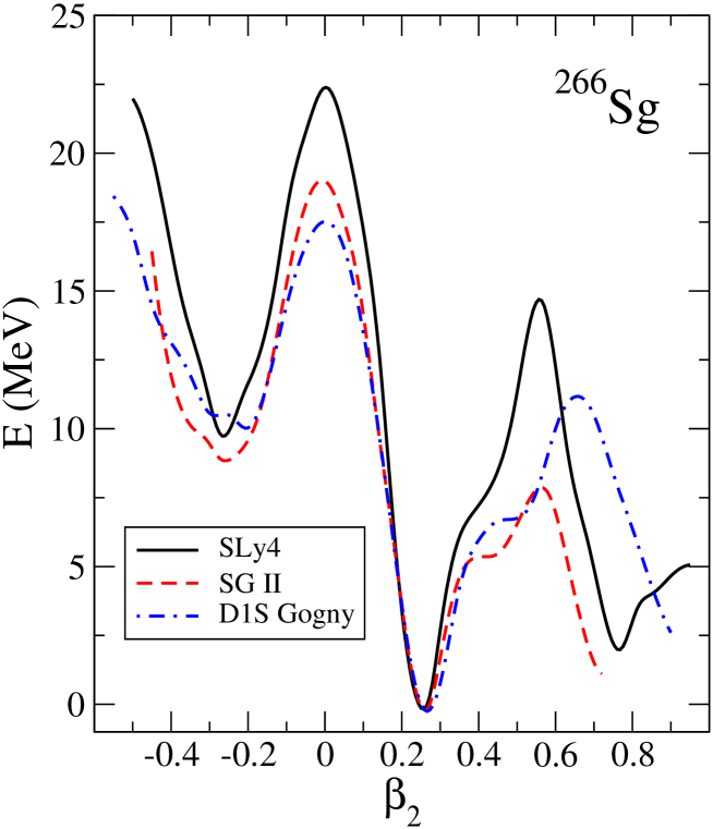
Figure 1: Deformation-energy curves for the ²⁶⁶Sg isotope obtained from constrained HF+BCS calculations with the Skyrme forces SLy4 chabanat and SGII sg2 , as well as with the D1S Gogny gogny interactions.

DECs are first shown in figure 1 for a selected isotope, ²⁶⁶Sg, which is representative of the nuclei in this mass region. The energies in figure 1 are relative to the ground state energy and are plotted as a function of the quadrupole deformation $\beta_{2}$. The results corresponding to the interaction of reference in this work (SLy4) show a ground state corresponding to a prolate shape at $\beta_{2}\approx 0.25$ and two excited configurations with oblate ($\beta_{2}\approx-0.25$) and superdeformed prolate ($\beta_{2}\approx 0.75$) shapes. The DECs obtained from other effective interactions are quite similar and, in particular, the prolate deformation of the ground state is very robust. To illustrate this feature, figure 1 shows also the results obtained with other standard Skyrme force, SGII from sg2 , as well as the results obtained with the finite-range D1S Gogny interaction gogny . The profile of the DEC turns out to be very similar to the DECs obtained for the other isotopes discussed in this work and agree also quite well with calculations performed with the Gogny D1S interaction gogny . In this work we calculate energy distributions of the GT strength and their corresponding half-lives for the ground state prolate configurations at $\beta_{2}\approx 0.25$. Deformations of parent and daughter decay partners are assumed to be the same in this work. This is a widely used approximation based on the spin-isospin character of the Gamow-Teller operator that does not contain any radial dependency. Thus, the spatial functions of parent and daughter wave functions are expected to be as close as possible to overlap maximally. As a result, transitions connecting different radial structures in the parent and daughter nuclei are suppressed. This is justified by the fact that core polarization effects in the daughter nuclei are negligible, as it can be seen, for example, from Gogny calculations gogny , where the DECs of parent and corresponding daughter isotopes considered in this work are practically the same with ground states at $\beta_{2}\approx 0.25$. Consequently, given the small polarization effects and the suppression of the overlaps with different deformations, only GT transitions between parent and daughter partners with like deformations are considered in the present work.

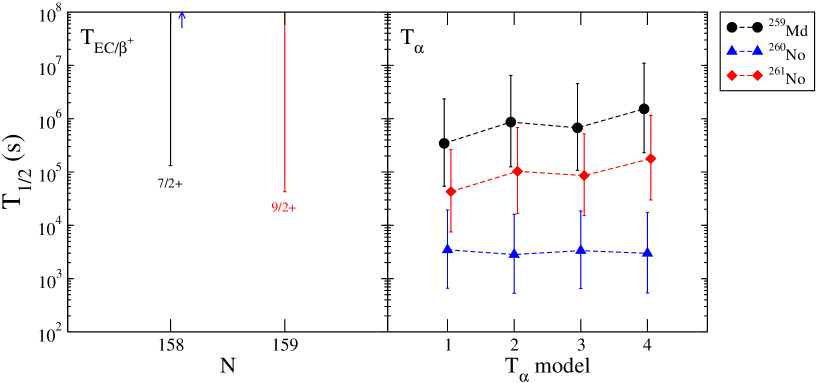
Figure 2: Calculated half-lives for ²⁵⁹Md, ²⁶⁰No, and ²⁶¹No isotopes. (left) Microscopic calculations of $T_{\beta^{+}/EC}$ for the ground state prolate configurations. $J^{\pi}$ is indicated for odd-$A$ isotopes. (right) $T_{\alpha}$ from four different phenomenological formulas, labeled from 1 up to 4 in the x axis (see text). $T_{1/2}$ in the y-axis is a short notation for both $T_{\beta^{+}/EC}$ and $T_{\alpha}$.

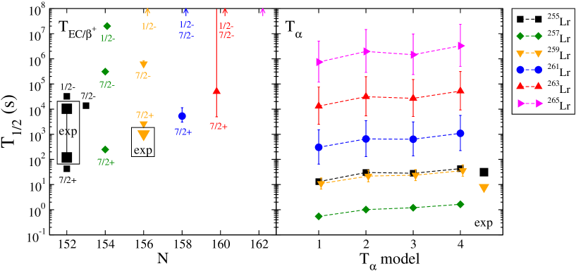
Figure 3: Same as in figure 2, but for the odd-$A$ Lr isotopes from ²⁵⁵Lr up to ²⁶⁵Lr.

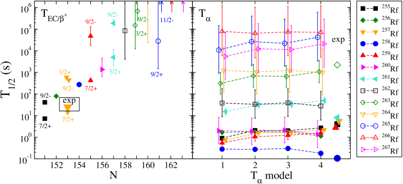
Figure 4: Same as in figure 2, but for ^255-267Rf isotopes.

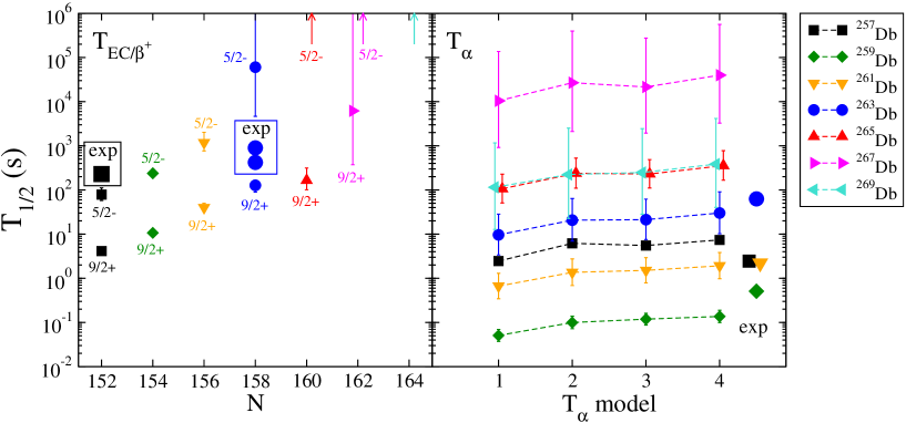
Figure 5: Same as in figure 2, but for the odd-$A$ Db isotopes from ²⁵⁷Db up to ²⁶⁹Db.

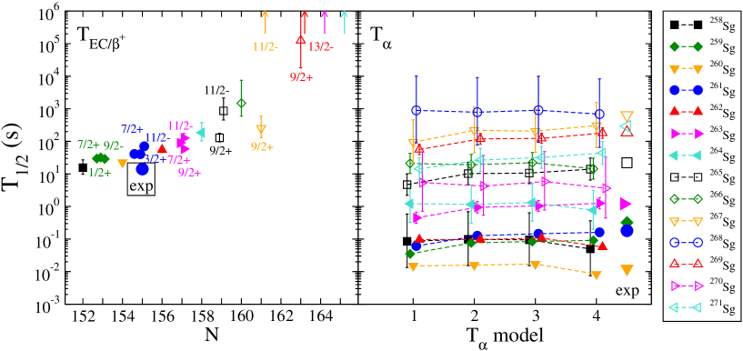
Figure 6: Same as in figure 2, but for ^258-271Sg isotopes.

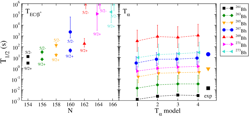
Figure 7: Same as in figure 2, but for the odd-$A$ Bh isotopes from ²⁶¹Bh up to ²⁷³Bh.

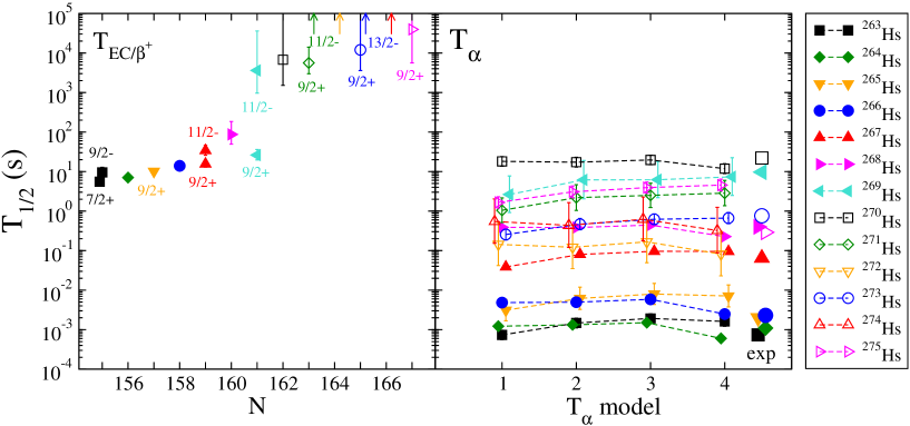
Figure 8: Same as in figure 2, but for ^263-275Hs isotopes.

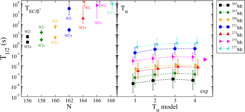
Figure 9: Same as in figure 2, but for the odd-$A$ Mt isotopes from ²⁶⁵Mt up to ²⁷⁷Mt.

In the next figures (figures 2 - 9) one can see the calculated half-lives $T_{\beta^{+}/EC}$ on the left-hand panels and $T_{\alpha}$ on the right-hand ones, grouped by isotopes. In the case of odd-$A$ nuclei, $T_{\beta^{+}/EC}$ are calculated for several $J^{\pi}$ values. For $T_{\alpha}$ there are calculations using the four models described above. The errors in the half-lives correspond to calculations using the extreme values of the $Q_{EC}$ and $Q_{\alpha}$ given by their experimental uncertainties in table LABEL:table_q. Experimental data for $T_{\beta^{+}/EC}$ ($T_{\alpha}$) are extracted and shown under the label ’exp’ in those cases where both the total experimental half-lives and the percentage of $\beta$ ($\alpha$) decay intensities are measured.

Figure 2 contains the results for Md ($Z=101$) and No ($Z=102$) isotopes. In this case the $\beta^{+}/EC$-decay half-lives are orders of magnitude larger than the corresponding $\alpha$-decay half-lives for a given isotope and have no special interest.

Figure 3 shows the results for the odd-$A$ Lr isotopes ($Z=103$). In this case $J^{\pi}$ is determined by the odd-proton state. The experimental $J^{\pi}$ assignments audi_12 are mostly uncertain (values within parenthesis) or estimated from systematic trends in neighboring nuclei (denoted with #). They are $J^{\pi}=(1/2^{-})_{\rm g.s.}$ and $(7/2^{-})$ in ²⁵⁵Lr, $J^{\pi}=(1/2^{-})$ in ²⁵⁷Lr, and $J^{\pi}=1/2^{-}$# in ²⁵⁹Lr. In the present calculations, states $1/2^{-}$, $7/2^{-}$ and $7/2^{+}$ very close in energy around the Fermi surface are obtained, and then, calculations for these three possibilities are performed. The $\beta^{+}/EC$-decay half-lives of the positive-parity states turn out to be much shorter than the corresponding half-lives of the negative-parity states. The latter are always orders of magnitude larger than the $\alpha$-decay half-lives, but the former can compete in some instances with $\alpha$-decay. Namely, in the case of the positive-parity states we obtain comparable $\beta^{+}/EC$- and $\alpha$-decay half-lives for ^255,263Lr isotopes. In the case of ²⁶¹Lr the difference is within a factor of 10, whereas for ²⁵⁹Lr the difference is already about two orders of magnitude.

Figure 4 corresponds to Rf isotopes ($Z=104$). Even-even and odd-$N$ isotopes are considered. In the case of odd-$N$ nuclei, $J^{\pi}$ is determined by the odd neutron state. The systematics of the $J^{\pi}$ in the various isotopes is not clear since each isotope has a different number of neutrons and the last neutron occupies a different orbital. Experimentally, the $J^{\pi}$ assignments are as follows, $J^{\pi}=(9/2^{-})_{\rm g.s.}$ and $5/2^{+}$# in ²⁵⁵Rf, $J^{\pi}=(1/2^{+})_{\rm g.s.}$ and $(11/2^{-})$ in ²⁵⁷Rf, $J^{\pi}=7/2^{+}\#_{\rm g.s.}$, $(3/2^{+})$ and $(9/2^{+})$ in ²⁵⁹Rf, $J^{\pi}=3/2^{+}\#_{\rm g.s.}$ and $9/2^{+}$# in ²⁶¹Rf, $J^{\pi}=3/2^{+}$# in ²⁶³Rf, and $J^{\pi}=3/2^{+}$# in ²⁶⁵Rf. In the calculations, various possibilities for the odd-neutron states are obtained including those mentioned above. $\beta^{+}/EC$-decay half-lives are performed for representative $J^{\pi}$ of both positive and negative parities. One can observe again that the $\beta^{+}/EC$-decay half-lives of the positive-parity states are shorter than the corresponding half-lives of the negative-parity states. For the positive-parity states, the half-lives of $\beta$- and $\alpha$-decays are similar in ^255,265Rf. In the case of ²⁵⁷Rf (²⁵⁶Rf) the $T_{\beta^{+}/EC}$ are within a factor of 10 (100) larger than $T_{\alpha}$.

In the case of the odd-$Z$ Db isotopes ($Z=105$) in figure 5, the experimental $J^{\pi}$ is found to be $J^{\pi}=(9/2^{+})_{\rm g.s.}$ and $(1/2^{-})$ in ²⁵⁷Db and $J^{\pi}=(9/2^{+})$ in ²⁶¹Db. These states are found in the calculations close to the Fermi surface, as well as $5/2^{-}$ states and half-lives are calculated for these options. Referring again to the positive-parity states that exhibit smaller half-lives than the negative ones, one can see that the half-lives of $\beta$- and $\alpha$-decays are comparable in ^257,265,267Db, while there is one order of magnitude of difference in ²⁶³Db and two orders in ^259,261Db.

Next we consider Sg ($Z=106$) isotopes in figure 6. The spin-parity experimental assignments of the odd isotopes are as follows: $J^{\pi}=1/2^{+}$# in ²⁵⁹Sg, $J^{\pi}=(3/2^{+})_{\rm g.s.}$ and $(11/2^{-})$ in ²⁶¹Sg, $J^{\pi}=7/2^{+}\#_{\rm g.s.}$ and $3/2^{+}$# in ²⁶³Sg, and $J^{\pi}=9/2^{+}\#_{\rm g.s.}$ and $3/2^{+}$# in ²⁶⁵Sg. In this case the half-lives $T_{\beta^{+}/EC}$ are quite similar for both parities in the lighter isotopes and they start to diverge from ²⁶⁷Sg. The $\beta$- and $\alpha$-decay half-lives are comparable in ²⁶⁷Sg, whereas they differ by about one order of magnitude in ²⁶⁵Sg and by two orders in ^258,263,266Sg.

The half-lives of Bh isotopes ($Z=107$) are shown in figure 7. The only experimental value of $J^{\pi}$ assigned is $(5/2^{-})$ in ²⁶¹Bh. The calculations give $5/2^{-}$ and $9/2^{+}$ states at the Fermi level and $\beta$-decay calculations are made for both of them. In the lighter isotopes considered there is not big difference between the $\beta^{+}/EC$-decay half-lives calculated with the different spin-parities. For isotopes heavier than $N=162$ the difference is much larger. The $\beta$- and $\alpha$-decay half-lives are comparable in ²⁶⁹Bh, they differ by one order of magnitude in ²⁶⁷Bh and by two orders of magnitude in ²⁶⁵Bh.

Even-even isotopes of Hs ($Z=108$) are shown in figure 8. The spin-parity experimental assignments are $7/2^{+}$# for ²⁶³Hs, $3/2^{+}\#_{\rm g.s.}$ and $9/2^{+}$# for ²⁶⁵Hs, $5/2^{+}$# for ²⁶⁷Hs, $9/2^{+}$# for ²⁶⁹Hs, and $3/2^{+}$# for ²⁷³Hs. Similar to the case of Sg isotopes, the $\beta^{+}/EC$-decay half-lives calculated with positive-parity states are very close to those from negative-parity states in the lighter isotopes up to $N=159$. Heavier isotopes show a more drastic dependence on the parity of the states. The $\beta$- and $\alpha$-decay half-lives differ by less than a factor of 10 in ²⁶⁹Hs and about two orders of magnitude in ^267,268Hs.

Finally, in Mt isotopes ($Z=109$), the half-lives plotted in figure 9 show that the difference between $T_{\alpha}$ and $T_{\beta^{+}/EC}$ is more than two orders of magnitude in all isotopes except ²⁷¹Mt, where it is about two orders.

From the above figures one can also learn about the uncertainties associated with different aspects of the calculations, in particular with the $Q_{EC}$ energies that are plotted as error bars and with the $J^{\pi}$ assignments in the case of odd-$A$ isotopes.

Tables LABEL:table2-LABEL:table4 summarize the main results obtained in this work regarding the comparison between the half-lives of the $\beta^{+}/EC$- and $\alpha$-decay modes. Table LABEL:table2 contains the calculated half-lives for the isotopes with comparable $T_{\beta^{+}/EC}$ and $T_{\alpha}$. Experimental values extracted from audi_12 are also shown when available. In the case of $T_{\alpha}$ the values shown correspond to the average value obtained from the four formulas considered in this work. SF in this mass region is another possible decay mode that might also compete with $\alpha$ and $\beta$ decay in some isotopes. For comparison, the available experimental half-lives for SF, $T_{SF}$, obtained from the total half-lives and percentage of the SF decay mode intensity from audi_12 are quoted in the last column of the table.

Table LABEL:table3 shows the same information as in table LABEL:table2, but for the isotopes whose $T_{\beta^{+}/EC}$ and $T_{\alpha}$ values are within a factor of ten. Similarly, table LABEL:table4 contains the information on the isotopes with $T_{\beta^{+}/EC}$ and $T_{\alpha}$ differing by about two orders of magnitude.

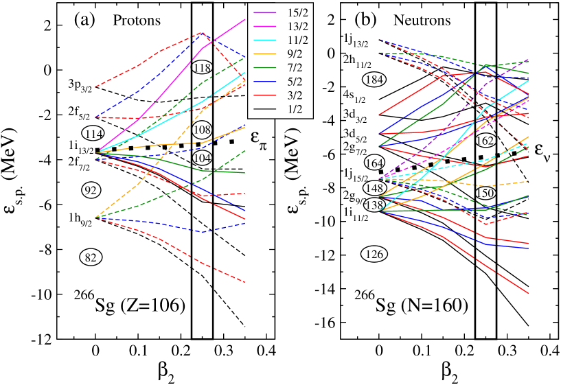
Figure 10: Single-particle energies obtained with SLy4 for (a) protons and (b) neutrons in ²⁶⁶Sg as a function of the quadrupole deformation $\beta_{2}$. The Fermi levels for protons ($\varepsilon_{\pi}$) and neutrons ($\varepsilon_{\nu}$) are depicted as thick dotted black lines. Positive-parity states are shown with solid lines, whereas negative-parity states are shown with dashed lines.

To understand why in the case of odd-$A$ isotopes the $T_{\beta^{+}/EC}$ for positive-parity states are always significantly lower than the same half-lives for negative-parity states, one has to analyze the different scenarios for the decay when the odd nucleon in the parent nucleus has a positive or a negative parity. This parity will determine the parity of all the states reached in the daughter nucleus (allowed transitions). For that purpose figure 10 shows a Nilsson-like diagram, where the single-particle energies are plotted as a function of the quadrupole deformation $\beta_{2}$ for protons (left) and neutrons (right) in the case of ²⁶⁶Sg with $Z=106$ and $N=160$. The calculations correspond to the Skyrme interaction SLy4. Fermi levels for protons ($\varepsilon_{\pi}$) and neutrons ($\varepsilon_{\nu}$) are plotted as thick dotted black lines. Positive-parity states are shown with solid lines, whereas negative-parity states are shown with dashed lines. The spherical shells are shown at $\beta_{2}=0$ with their spherical quantum numbers. The boxes centered at $\beta_{2}=0.25$ correspond to the regions of interest determined by the quadrupole deformation of the equilibrium ground state in this mass region. The color code used to plot the different components of the angular momenta is also shown.

The spherical shells involved in the $\beta^{+}/EC$-decay in increasing order of energy are the following: $h_{9/2},\ f_{7/2},\ i_{13/2},\ f_{5/2},\ p_{3/2}$ for protons and $i_{11/2},\ g_{9/2},\ j_{15/2},\ g_{7/2},\ d_{5/2},\ d_{3/2},\ s_{1/2},\ h_{11/2},\ j_{13/2}$ for neutrons. In this analysis it is sufficient to focus on the states in the vicinity of the Fermi energy because only low-lying transitions involving the odd nucleon are relevant to calculate half-lives in nuclei with low $Q$-energies, which is the case of the isotopes studied here. In the $\beta^{+}/EC$-decay one proton is transformed into one neutron. In the case of odd-proton isotopes, the odd-proton is directly involved in the low-lying transitions below the $Q$-window that determine the $\beta^{+}/EC$-decay half-lives. In the case of odd-neutron isotopes, the low-lying GT excitations corresponding to $\beta^{+}/EC$-decay involve proton states in the vicinity of the Fermi level that match the allowed quantum-numbers given by the odd neutron.

Focusing on the proton single-particle energies within the box around $\beta_{2}=0.25$, one can see that among the odd-proton isotopes considered, Lr ($Z=103$) would have the odd proton placed in one of the orbitals $7/2^{-}$, $7/2^{+}$, and $1/2^{-}$ close to the Fermi energy. They originate in the spherical shells $h_{9/2},\ i_{13/2},\ f_{5/2}$, respectively. In the case of Db ($Z=105$) and Bh ($Z=107$), the states involved would be $5/2^{-}\,(f_{7/2})$ and $9/2^{+}\,(i_{13/2})$, whereas in the case of Mt($Z=109$) one finds the states $9/2^{+}\,(i_{13/2})$, $9/2^{-}\,(h_{9/2})$, $3/2^{-}\,(f_{5/2})$, and $11/2^{+}\,(i_{13/2})$ close to the Fermi level. All of above states have been considered in the decay of these odd-$A$ isotopes. Therefore, in the odd-proton isotopes, the states mentioned above would decay into neutron states in the vicinity of the neutron Fermi energy, which is shown in the right panel of figure 10 within the black box centered at $\beta_{2}=0.25$. For neutron numbers between $N$=150-162 the states involved are $9/2^{-}\,(j_{15/2})$, $7/2^{+}\,(g_{9/2})$, $9/2^{+}\,(i_{11/2})$, $1/2^{+}\,(d_{5/2})$, $3/2^{+}\,(g_{7/2})$, and $11/2^{-}\,(j_{15/2})$. Beyond $N$=162, new states appear with $13/2^{-}\,(j_{15/2})$, $9/2^{+}\,(g_{9/2})$, $5/2^{+}\,(g_{7/2})$, $3/2^{+}\,(d_{5/2})$, $3/2^{-}\,(h_{11/2})$, and $1/2^{-}\,(h_{11/2},j_{13/2})$.

Then, it is easy to understand that the transitions involving the positive-parity proton states, namely $7/2^{+}$ and $9/2^{+}$, would match the neutron states $5/2^{+}$, $7/2^{+}$, and $9/2^{+}$, while the negative-parity proton states $5/2^{-}$ cannot match the $9/2^{-}$, $11/2^{-}$ or $13/2^{-}$ and only in the heavier isotopes the $9/2^{-}$ proton states states can match the $9/2^{-}$ and $11/2^{-}$ neutron states. This explains qualitatively why the decays from even-parity states are much faster than the decays from odd-parity states. In the case of odd-neutron isotopes, the argument is similar, but now, the odd neutron in the parent nucleus determines the proton states involved in the transitions.

The comparison of the calculations with the available experimental half-lives in both cases $T_{\beta^{+}/EC}$ and $T_{\alpha}$ is in general quite satisfactory, which helps to be confident in the reliability of the calculations. More specifically, in the case of $\beta^{+}/EC$-decay, the experimental $T_{\beta^{+}/EC}$ in ²⁵⁵Lr lies within the calculated half-lives with positive- or negative-parity states, whereas in the case of ²⁵⁵Lr and ²⁵⁷Rf the experiment is very close to the calculation with the $7/2^{+}$ state. On the other hand, in ²⁵⁷Db, the experiment is closer to the calculation with negative parity and in ²⁶³Db the experiment lies between the predictions with positive or negative parities. Finally, in ²⁶¹Sg the experiment is close to the calculations with both parities. In the case of $\alpha$-decay the experimental information on half-lives is more abundant. In general, the predictions of the different formulas considered agree within one order of magnitude with the measurements.

IV Conclusions

In this work, the $\beta^{+}/EC$-decay half-lives of some selected even-even and odd-$A$ isotopes in the region $Z=101-109$ and $N=151-168$ are studied. Namely, ²⁵⁹Md, ^260,261No, odd ^255-265Lr, ^255-267Rf, odd ^257-269Db, ^258-271Sg, odd ^261-273Bh, ^263-275Hs, and odd ^265-277Mt. The microscopic formalism used to describe the nuclear structure of the decay partners is based on a deformed Skyrme HF+BCS approach.

Uncertainties in the experimental $Q_{EC}$ energies are translated into uncertainties of the half-lives calculated with them. In the case of odd-$A$ nuclei, different $J^{\pi}$ assignments are considered to learn about their influence on the final half-lives. It is found that in odd-$A$ isotopes the $T_{\beta^{+}/EC}$ for the positive-parity states are always shorter than the $T_{\beta^{+}/EC}$ for the negative-parity states. The results for $T_{\beta^{+}/EC}$ are compared with the $\alpha$-decay half-lives $T_{\alpha}$ obtained from phenomenological formulas using experimental $Q_{\alpha}$ energies and their uncertainties. The agreement between the calculated and the available experimental half-lives in both cases $T_{\beta^{+}/EC}$ and $T_{\alpha}$ is found to be always within a factor of 10, granting the category of trustable predictions.

$T_{\alpha}$ are in most cases lower than the corresponding $T_{\beta^{+}/EC}$ for a given isotope. This difference is about two orders of magnitude in ²⁵⁹Lr, ²⁵⁶Rf, ^259,261Db, ^258,263,266Sg, ²⁶⁵Bh, ^267,268Hs, and ²⁷¹Mt. In the cases of ²⁶¹Lr, ²⁵⁷Rf, ²⁶³Db, ²⁶⁵Sg and ²⁶⁷Bh the difference is only about one order of magnitude. Finally, the isotopes ^255,263Lr, ^255,265Rf, ^257,265,267Db, ²⁶⁷Sg, ²⁶⁹Bh, and ²⁶⁹Hs have comparable values of the half-lives for the $\beta^{+}/EC$- and $\alpha$-decay modes. Therefore, these different modes will compete in the latter cases favoring new branches of decay in the $\beta^{+}/EC$ direction that have not yet been sufficiently studied. This opens new possibilities to reach unexplored roads towards the predicted islands of stability.

Table 1: Experimental $Q_{\rm EC}$ and $Q_{\alpha}$ energies (MeV) from AME2012 audi_12

Nucleus	$Q_{\rm EC}$	$Q_{\alpha}$	Nucleus	$Q_{\rm EC}$	$Q_{\alpha}$	Nucleus	$Q_{\rm EC}$	$Q_{\alpha}$
259Md	0.0 $\pm$ 0.3	7.11 $\pm$ 0.20
260No	-0.9 $\pm$ 0.4	7.70 $\pm$ 0.20	261No	0.0 $\pm$ 0.5	7.44 $\pm$ 0.20
255Lr	3.140 $\pm$ 0.023	8.556 $\pm$ 0.007	257Lr	2.36 $\pm$ 0.05	9.01 $\pm$ 0.03	259Lr	1.74 $\pm$ 0.12	8.58 $\pm$ 0.07
261Lr	1.11 $\pm$ 0.28	8.14 $\pm$ 0.20	263Lr	0.60 $\pm$ 0.57	7.68 $\pm$ 0.20	265Lr	-	7.23 $\pm$ 0.20
255Rf	4.38 $\pm$ 0.12	9.055 $\pm$ 0.004	256Rf	2.48 $\pm$ 0.08	8.926 $\pm$ 0.015	257Rf	3.26 $\pm$ 0.05	9.083 $\pm$ 0.008
258Rf	1.56 $\pm$ 0.11	9.19 $\pm$ 0.03	259Rf	2.51 $\pm$ 0.10	9.13 $\pm$ 0.07	260Rf	0.87 $\pm$ 0.24	8.90 $\pm$ 0.20
261Rf	1.76 $\pm$ 0.21	8.65 $\pm$ 0.05	262Rf	0.29 $\pm$ 0.30	8.49 $\pm$ 0.20	263Rf	1.06 $\pm$ 0.34	8.25 $\pm$ 0.15
264Rf	-0.20 $\pm$ 0.60	8.04 $\pm$ 0.30	265Rf	0.46 $\pm$ 0.71	7.81 $\pm$ 0.30	266Rf	-1.5 $\pm$ 0.7	7.55 $\pm$ 0.30
267Rf	-	7.89 $\pm$ 0.30
257Db	4.34 $\pm$ 0.20	9.026 $\pm$ 0.020	259Db	3.63 $\pm$ 0.09	9.62 $\pm$ 0.05	261Db	2.93 $\pm$ 0.12	9.22 $\pm$ 0.10
263Db	2.32 $\pm$ 0.25	8.83 $\pm$ 0.15	265Db	1.80 $\pm$ 0.42	8.50 $\pm$ 0.10	267Db	0.63 $\pm$ 0.71	7.92 $\pm$ 0.30
269Db	-	8.49 $\pm$ 0.30
258Sg	3.45 $\pm$ 0.51	9.62 $\pm$ 0.30	259Sg	4.57 $\pm$ 0.13	9.804 $\pm$ 0.021	260Sg	2.88 $\pm$ 0.10	9.901 $\pm$ 0.010
261Sg	3.76 $\pm$ 0.11	9.714 $\pm$ 0.015	262Sg	2.11 $\pm$ 0.15	9.600 $\pm$ 0.015	263Sg	3.08 $\pm$ 0.19	9.40 $\pm$ 0.06
264Sg	1.42 $\pm$ 0.37	9.21 $\pm$ 0.20	265Sg	2.31 $\pm$ 0.26	9.05 $\pm$ 0.11	266Sg	0.88 $\pm$ 0.37	8.80 $\pm$ 0.10
267Sg	1.76 $\pm$ 0.50	8.63 $\pm$ 0.21	268Sg	-0.2 $\pm$ 0.7	8.30 $\pm$ 0.30	269Sg	0.67 $\pm$ 0.77	8.70 $\pm$ 0.05
270Sg	-0.7 $\pm$ 0.8	8.99 $\pm$ 0.30	271Sg	-	8.89 $\pm$ 0.11
261Bh	5.13 $\pm$ 0.21	10.50 $\pm$ 0.05	263Bh	4.31 $\pm$ 0.32	10.08 $\pm$ 0.30	265Bh	3.56 $\pm$ 0.26	9.68 $\pm$ 0.21
267Bh	2.93 $\pm$ 0.38	9.23 $\pm$ 0.20	269Bh	1.67 $\pm$ 0.52	8.57 $\pm$ 0.30	271Bh	1.23 $\pm$ 0.73	9.49 $\pm$ 0.16
273Bh	0.62 $\pm$ 0.90	9.06 $\pm$ 0.30
263Hs	5.22 $\pm$ 0.33	10.73 $\pm$ 0.05	264Hs	3.51 $\pm$ 0.18	10.59 $\pm$ 0.02	265Hs	4.55 $\pm$ 0.24	10.47 $\pm$ 0.11
266Hs	3.03 $\pm$ 0.17	10.346 $\pm$ 0.016	267Hs	3.89 $\pm$ 0.28	10.037 $\pm$ 0.013	268Hs	2.02 $\pm$ 0.48	9.623 $\pm$ 0.016
269Hs	3.11 $\pm$ 0.39	9.37 $\pm$ 0.16	270Hs	0.86 $\pm$ 0.38	9.05 $\pm$ 0.04	271Hs	1.78 $\pm$ 0.53	9.51 $\pm$ 0.11
272Hs	0.22 $\pm$ 0.74	9.78 $\pm$ 0.20	273Hs	1.34 $\pm$ 0.83	9.73 $\pm$ 0.05	274Hs	-0.1 $\pm$ 0.9	9.57 $\pm$ 0.20
275Hs	0.93 $\pm$ 0.84	9.44 $\pm$ 0.05
265Mt	5.78 $\pm$ 0.45	11.12 $\pm$ 0.40	267Mt	5.14 $\pm$ 0.51	10.87 $\pm$ 0.40	269Mt	4.72 $\pm$ 0.48	10.53 $\pm$ 0.40
271Mt	3.33 $\pm$ 0.44	9.91 $\pm$ 0.20	273Mt	2.53 $\pm$ 0.60	10.60 $\pm$ 0.30	275Mt	2.01 $\pm$ 0.75	10.21 $\pm$ 0.15
277Mt	1.28 $\pm$ 0.94	9.71 $\pm$ 0.20

Table 2: Experimental audi_12 and calculated $T_{\beta^{+}/EC}$ [s] and $T_{\alpha}$ [s] for isotopes with comparable half-lives. Experimental half-lives for spontaneous fission audi_12 , $T_{SF}$ [s], are also shown for comparison.

Nucleus	$T_{\beta^{+}/EC}$			$T_{\alpha}$			$T_{SF}$
	exp.	calc.		exp.	calc.		exp.
255Lr	120	42.6		42	28.6
263Lr		50231			30925
255Rf		7.2		3.5	1.9		3.2
265Rf		28211			25260		396
257Db	230	4.1		2.5	5.4		46
265Db		165			233
267Db		6192			24700		16560
267Sg		254		636	206		130
269Bh		192			770
269Hs		26.1		27	5.6

Table 3: Same as in Table LABEL:table2, but for isotopes with $T_{\beta^{+}/EC}$ and $T_{\alpha}$ half-lives differing by about one order of magnitude.

Nucleus	$T_{\beta^{+}/EC}$			$T_{\alpha}$			$T_{SF}$
	exp.	calc.		exp.	calc.		exp.
261Lr		5414			670
257Rf	25.4	14.3		6.0	1.6		371
263Db	420	127		78.4	20.4		51.8
265Sg		128		18.4	9.9		184
267Bh		44.8		22	6.4

Table 4: Same as in Table LABEL:table2, but for isotopes with $T_{\beta^{+}/EC}$ and $T_{\alpha}$ half-lives differing by about two orders of magnitude.

Nucleus	$T_{\beta^{+}/EC}$			$T_{\alpha}$			$T_{SF}$
	exp.	calc.		exp.	calc.		exp.
259Lr	1033	2609		8.0	23.1		28.2
256Rf		79.1			1.6		0.007
259Db		10.7		0.5	0.10
261Db		40.1		16.7	1.4		6.2
258Sg		15.6		0.14	0.08		0.034
263Sg		58.8		1.1	0.9		7.2
266Sg		1483			19.1		0.46
265Bh		16.9		1.2	0.33
267Hs		15.5		0.07	0.08		0.28
268Hs		86.9		1.4	0.36
271Mt		28.6		0.4	0.36