The Dynamics and Infrared Spectrocopy of Monomeric and Dimeric Wild Type and Mutant Insulin

Abstract

The infrared spectroscopy and dynamics of -CO labels in wild type and mutant insulin monomer and dimer are characterized from molecular dynamics simulations using validated force fields. It is found that the spectroscopy of monomeric and dimeric forms in the region of the amide-I vibration differs for residues B24-B26 and D24-D26, which are involved in dimerization of the hormone. Also, the spectroscopic signatures change for mutations at position B24 from phenylalanine - which is conserved in many organisms and known to play a central role in insulin aggregation - to alanine or glycine. Using three different methods to determine the frequency trajectories - solving the nuclear Schrödinger equation on an effective 1-dimensional potential energy curve, instantaneous normal modes, and using parametrized frequency maps - lead to the same overall conclusions. The spectroscopic response of monomeric WT and mutant insulin differs from that of their respective dimers and the spectroscopy of the two monomers in the dimer is also not identical. For the WT and F24A and F24G monomers spectroscopic shifts are found to be $\sim 20$ cm^-1 for residues (B24 to B26) located at the dimerization interface. Although the crystal structure of the dimer is that of a symmetric homodimer, dynamically the two monomers are not equivalent on the nanosecond time scale. Together with earlier work on the thermodynamic stability of the WT and the same mutants it is concluded that combining computational and experimental infrared spectroscopy provides a potentially powerful way to characterize the aggregation state and dimerization energy of modified insulins.

a an the of on at with for and in into from by without University of Basel]Department of Chemistry, University of Basel, Klingelbergstrasse 80 , CH-4056 Basel, Switzerland. University of Basel]Department of Chemistry, University of Basel, Klingelbergstrasse 80 , CH-4056 Basel, Switzerland.

1 Introduction

Insulin is a small, aggregating protein with an essential role in regulating glucose uptake in cells. Physiologically, it binds to the insulin receptor (IR) in its monomeric form but thermodynamically the dimer is more stable for the wild type (WT) protein.^{1, 2, 3} The storage form is that of a zinc-bound hexamer with either two or four Zn atoms.⁴ Hence, to arrive at the functionally relevant monomeric stage, insulin has to cycle through at least two dissociation steps: from the hexamer to three dimers and from the dimer to the monomer.

For pharmacological applications the dimer$\leftrightarrow$monomer equilibrium is particularly relevant because for safe insulin administration this equilibrium needs to be tightly controlled. However, reliable experimental physico-chemical information about the relative stabilization of insulin monomer and dimer, which is $-7.2$ kcal/mol in favour of the dimer,¹ is only available for the WT and the barrier between the two states is unknown. For mutant insulins, there is no such quantitative information from experiments. On the other hand, insulin has become a paradigm for studying coupled folding and binding,⁵ whether or not association proceeds along one or multiple pathways,^{6, 7} and for the role of water in protein association.^{8, 9, 10} Most of these studies were based on atomistic molecular dynamics (MD) simulations and provided remarkable insight into functionally relevant processes for this important system.

Infrared spectroscopy has been proposed¹¹ and recently demonstrated¹² to provide a way to quantify protein-ligand binding strengths through observation of spectroscopic shifts. The physical foundation for this is the Stark effect which is based on the electrostatic interaction between a local reporter and the electric field generated by its environment. Using accurate multipolar force fields¹³ it was possible to assign the structural substates in photodissociated CO from Myoglobin¹⁴ whereas more standard, point charge-based force fields are not suitable for such investigations.¹⁵

The frequency trajectory of a local reporter can be followed in different ways. One of them uses so-called parametrized “frequency maps” which are precomputed for a given reporter from a large number of ab initio calculations.^{16, 17, 18, 19} Alternatively, the sampling of the configurations and computing frequencies for given snapshots can also be done using the same energy function (“scan”). In this approach, the MD simulations are carried out with the same energy function that is also used for the analysis, which is typically a multipolar representation for the electrostatics around the spectroscopic probe and an anharmonic (Morse) for the bonded terms.^{20, 21} On each snapshot, the local frequency is determined from either an instantaneous normal mode (INM) calculation or by solving the 1D or three-dimensional nuclear Schrödinger equation.²²

Here, the WT proteins and two mutants at position B24 (Phe) are considered. Phenylalanine B24 is located at the dimerization interface and invariant among insulin sequences.²³ Compared with the WT, the SerB24,^{24, 25} LeuB24,²⁶ and HisB24²⁷ analogues show reduced binding potency towards the receptor. On the other hand, substitutions such as GlyB24, D-AlaB24, or D-HisB24 are well tolerated as judged from their binding affinity. Nevertheless, substitutions such as GlyB24 (F24G) or AlaB24 (F24A) were found to have reduced stability of the modified insulin dimer, both from simulations and experiment,^{8, 28, 29} and these are the variants considered in the present work.

In the present work the infrared spectrum in the amide-I stretch region is studied for wild type (WT) and two mutant insulins in their monomeric and dimeric states using accurate multipolar force fields. The IR lineshapes are calculated from frequency trajectories calculated by using a normal mode analysis, solving the Schrödinger equation from a 1-d scan along the amide-I normal mode and using previously parametrized maps. First, the methods are presented. Then, results for IR lineshapes and frequency correlation functions from scanning along the amide-I normal mode are presented and discussed and compared with the two other approaches. Finally, conclusions are drawn.

2 Methods

2.1 Molecular Dynamics Simulations

All molecular dynamics (MD) simulations were carried out using the CHARMM³⁰ package together with CHARMM36³¹ force field including the CMAP correction^{32, 33} and multipoles up to quadrupole on the [CONH]-part of the backbone.^{21, 34} The X-ray crystal structure of the insulin dimer was solvated in a cubic box ($75^{3}$ ų) of TIP3P³⁵ water molecules, which leads to a total system size of 40054 atoms. For the monomer simulations, chains A and B were retained and also solvated in a water box ($75^{3}$ ų ), the same box size as the dimer. In these simulations the multipolar^{36, 13, 21, 34} force field is used for the entire amide groups and all CO bonds are treated with a Morse potential $V(r)=D_{e}(1-\exp(-\beta(r-r_{e})))^{2}$. The parameters are $D_{e}=141.666$ kcal/mol, $\beta=2.112$ Å^-1 and $r_{0}=1.231$ Å.

Hydrogen atoms were included and the structures of all systems were minimized using 2000 steps of steepest descent (SD) and 200 steps of Newton Raphson (ABNR) followed by 20 ps of equilibration MD at 300 K. A Velocity Verlet integrator³⁷ and Nosé-Hoover thermostat^{38, 39} were employed in the $NVT$ simulations. Then production runs (1 ns or 5 ns) were carried out in the $NpT$ ensemble, with coordinates saved every 10 fs for subsequent analysis. For the $NpT$ simulations an Andersen and Nosé-Hoover constant pressure and temperature algorithm was used^{40, 41, 39} together with a leapfrog integrator.⁴² a coupling strength for the thermostat of 5 ps and a damping coefficient of 5 ps^-1. All bonds involving hydrogen atoms were constrained using SHAKE⁴³. Nonbonded interactions were treated with a switching function⁴⁴ between 10 and 14 Å and for the electrostatic interactions, the Particle Mesh Ewald (PME) method was used with grid size spacing of 1 Å, characteristic reciprocal length $\kappa=0.32$ Å^-1, and interpolation order 4.⁴⁵ Figure 1A shows the insulin dimer highlighting some of the CO labels studied in the current work with particular attention to the -CO labels at the protein-protein interface (B24-B26) and (D24-D26).

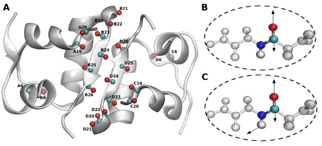
Figure 1: Panel A: Structure of wild type insulin dimer with the -CO labels that are specifically probed in the present work. The dimerization interface involves residues B24-B26 and D24-D26. Panels B and C show the displacement vectors for the two scan approaches considered to construct 1D potentials along the CO and CONH directions, respectively.

2.2 Frequencies from Solving the 1d Schrödinger Equation: Scan

Anharmonic transition frequencies can be determined from calculating the 1-d potential energy along the CO or amide-I normal mode (from a normal mode analysis on N-methyl acetamide (NMA) in the gas phase) and solving the nuclear Schrödinger equation (SE) for each snapshot using a discrete variable representation (DVR) approach⁴⁶. It was shown previously for NMA⁴⁷ that frequency trajectories obtained from solving the SE on the 1-d PES scanned along either the CONH (amide-I) or the CO mode (see Figure 1B and C) result in similar decay times with frequencies shifted by some $\sim 15$ cm^-1. Here, scans were performed for each snapshot for 61 points along the CO normal mode vector around the minimum energy structure using the same energy function as that used for the MD simulations, i.e. a multipolar representation of the electrostatics and an anharmonic Morse potential for the CO-bond. An RKHS representation of the 1-d PES is then constructed from these energies and the SE is solved on a grid ($-0.53$ Å $<r<0.53$ Å ) using a reduced mass of 1 amu.⁴⁷ For direct comparison, scans along the amide-I mode were also carried out for selected residues.

2.3 Instantaneous Normal Mode

The instantaneous (harmonic) frequencies for each snapshot of the trajectory from the $NPT$ simulation were calculated for the same snapshots for which the scan along the CO normal mode was carried out, see above. Such instantaneous normal modes (INM) are determined by minimizing CO or [CONH] while keeping the environment (protein plus solvent) fixed. Next, normal modes were calculated from the “vibran” facility in CHARMM.

2.4 The Amide I Frequency Maps

The frequency map used in the present work is that parametrized by Tokmakoff and coworkers.¹⁹ It requires MD simulations to be run with fixed CO bond length and is based on the expression

$$\omega_{i}=\omega_{0}+aE_{C_{i}}+E_{{N}_{i}}$$ (1)

where $\omega_{i}$ is the instantaneous frequency for the $i$th vibrational label, $E_{C_{i}}$ is the electric field on the C atom in the $i$th label along the C=O bond direction, and $E_{N_{i}}$ is that on the N atom. Parameters $\omega_{0}$, $a$, and $b$ were fitted such that they optimally reproduce the experimental IR absorption spectra of NMAD. The optimized backbone map is¹⁹

$$\omega_{i}=1677.9+2557.8E_{\rm C_{i}}-1099.5E_{N_{i}}$$ (2)

In this equation, $\omega_{i}$ is in cm^-1 and $E_{C_{i}}$ and $E_{N_{i}}$ are in atomic units.

2.5 Frequency Fluctuation Correlation Function and Lineshape

From the harmonic or anharmonic frequency trajectory $\omega_{i}(t)$ or $\nu_{i}(t)$ for label $i$ its frequency fluctuation correlation function, $\langle\delta\omega(0)\delta\omega(t)\rangle$ is computed. Here, $\delta\omega(t)=\omega(t)-\langle\omega(t)\rangle$ and $\langle\omega(t)\rangle$ is the ensemble average of the transition frequency. From the FFCF the line shape function

$$g(t)=\int_{0}^{t}\int_{0}^{\tau^{{}^{\prime}}}\langle\delta\omega(\tau^{{}^{\prime\prime}})\delta\omega(0)\rangle d\tau^{{}^{\prime\prime}}d\tau^{{}^{\prime}}.$$ (3)

is determined within the cumulant approximation. To compute $g(t)$, the FFCF is numerically integrated using the trapezoidal rule and the 1D-IR spectrum is calculated according to⁴⁸

$$I(\omega)=2\Re\int^{\infty}_{0}e^{i(\omega-\langle\omega\rangle)t}e^{-g(t)}e^{-\frac{t\alpha}{2T_{1}}}dt$$ (4)

where $\langle\omega\rangle$ is the average transition frequency obtained from the distribution, $T_{1}=0.45$ ps is the vibrational relaxation time and $\alpha=0.5$ is a phenomenological factor to account for lifetime broadening.⁴⁸

For extracting time information from the FFCF, $\langle\delta\omega(t)\delta\omega(0)\rangle$ is fitted to an empirical expression⁴⁹

$$\langle\delta\omega(t)\delta\omega(0)\rangle=a_{1}\cos(\gamma t)e^{-t/\tau_{1}}+\sum_{i=2}^{n}a_{i}e^{-t/\tau_{i}}+\Delta_{0}$$ (5)

where $a_{i}$ are amplitudes, $\tau_{i}$ are decay times and $\Delta_{0}$ is an offset for long correlation times. The $\cos-$term allows to capture a short-time recurrence (anticorrelation) that may or may not be present in the correlation function. This minimum at very short time ($t\sim 0.1$ ps) is known from previous simulations⁵⁰ and can be related to the strength of the interaction between solute and solvent^{49, 20, 21, 22} or between the spectroscopic probe and its environment (as in the present case). The decay times $\tau_{i}$ of the frequency fluctuation correlation function reflect the characteristic time-scale of the solvent fluctuations to which the solute degrees of freedom are coupled. In most cases the FFCFs were fitted to an expression containing two decay times using an automated curve fitting tool from the SciPy library.⁵¹ Only if the quality of the resulting fit was evidently insufficient, a third decay time was included.

3 Results

The results section is structured as follows. First, a brief account is given of representative structures along the trajectories for the different simulation conditions used. Next, the amide-I spectroscopy for the WT monomer and dimer using the “scan” approach is given. This is followed by the spectroscopy for the mutant monomer and dimer compared with the WT systems. Then, a comparative discussion of the results for WT and mutant monomer and dimer is given for the three methods to determine the frequency trajectories (“scan”, “INM” and “map”) and finally, the FFCFs from the “scan” and “INM” frequency trajectories are discussed.

3.1 Structural Characterization

The root mean squared deviation between the reference X-ray structure and those of the monomer and dimer structure of the WT protein in solution is reported in Figure 2. Typically, the RMSD is around 1.5 Å which is indicative of a stable simulation on the nanosecond time scale. Such RMSD values have also been reported from simulations in smaller water boxes.^{52, 3}

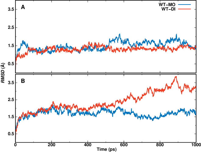
Figure 2: The structural RMSD between the reference X-ray structure and the Wild type monomer and dimer insulin for A) flexible and B) constrained CO.

With constrained CO (as is required for using the frequency maps) the structure of the monomer is equally well maintained whereas for the dimer it starts to deviate from the reference structure by $\sim 3$ Å after 0.8 ns. This is indicative of structural changes which involve separation of the terminal of chain B (PheB1 and AlaB30) from each other. A similar but less pronounced effect was also observed for chain D between PheD1 and AlaD30.

3.2 Amide-I Spectroscopy Using Scan for WT and Mutant Monomer and Dimer

To set the stage, the Amide-I spectroscopy for the WT monomer and dimer is discussed from frequency trajectories obtained by scanning along the CO normal mode for each snapshot. Figure 3 reports the lineshapes for all CO-labels for the WT monomer. Lineshapes for chain A are solid lines and those for chain B are dashed. The overall lineshape for the monomer (black solid line) is centered at 1630.5 cm^-1 and has a full width at half maximum of $\sim 30$ cm^-1, compared with a center frequency of $\sim 1650$ cm^-1 and a FWHM of $\sim 30$ cm^-1 from experiments.^{53, 54} When comparing the position of the frequency maximum it should be noted that the present parametrization is for NMA and slight readjustments of the Morse parameters could be made to yield quantitative agreement. However, for the present purpose such a step was deemed unnecessary.

On the other hand, scanning the 1-dimensional potential along the amide-I normal mode shifts the frequencies by about 30 cm^-1 to the blue (see Figure S1A). The correlation between scanning along the CO and amide-I normal modes is high, as Figure S1C shows. In addition, the full 1D infrared spectrum was also calculated from scanning along the amide-I normal mode (Figure S2) and confirms the overall shift to the blue by 25 cm^-1 while maintaining the shape and width of the total lineshape from scanning along the CO normal mode.

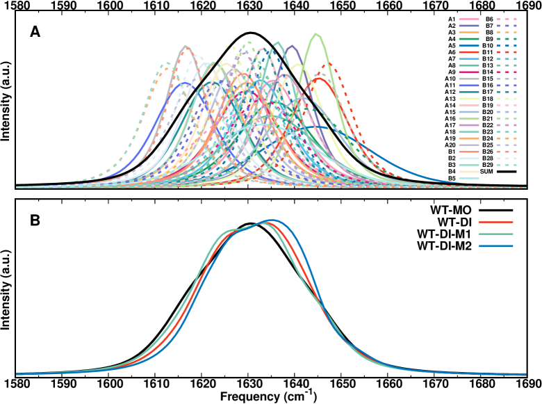
Figure 3: Panel A: 1D IR spectra for all residues in WT monomer based on “scan” for the frequency calculation. The labels for the individual line shapes are given in the panel and the overall sum is the solid black line. Panel B: The total lineshape for all CO probes of the monomer (black) compared with that of M1 (green) and M2 (blue) within the dimer and with the dimer itself (red). All lineshapes are scaled to the same maximum intensity. The line shapes are determined from 1 ns simulations and the snapshots analyzed are separated by 10 fs.

Most notably, the center frequencies for each of the labels cover a range from 1612.5 cm^-1 (residues B24, B29) to 1647.5 cm^-1 (residue B11) although the bonded potential (Morse) for the CO stretch is the same for all 51 labels. Hence, the multipolar charge distribution used for the electrostatics and its interaction with the environment leads to the displacements of the center frequencies. The linewidths also vary for the -CO probes at the different locations along the polypeptide chain and cover a range from 10 cm^-1 (Residues A10, A16, A18, B18, B21) to 28 cm ^-1 (Residue A5).

Selected lineshapes for the monomer and each of the two monomers within insulin dimer from scanning along the CO normal mode are reported in Figures 4 and S3 and the individual and total lineshapes for the two monomers (M1 and M2) within the dimer are shown in Figures S4 and S5. For the dimer it is noted that some probes at symmetry related positions within the dimer structure typically have their maxima at different frequencies. In other words, structurally related -CO probes sample different environments in the hydrated system at room temperature. The overall lineshapes of M1 and M2 are directly compared with that of the isolated monomer and the dimer in Figure 3B. The lineshape of M1 and M2 differ which confirms the asymmetry noted earlier from X-ray experiments.^{4, 55} Also, the spectroscopy of the isolated monomer differs from that of M1 and M2 within the dimer. Notably, the -CO groups involved in the hydrogen bonding motif of the insulin dimer (B24 to B26 and D26 to D24) display frequency maxima that differ by $\sim 10$ cm^-1. Other -CO reporters, such as B20 and D20, have their maxima only $\sim 5$ cm^-1 apart.

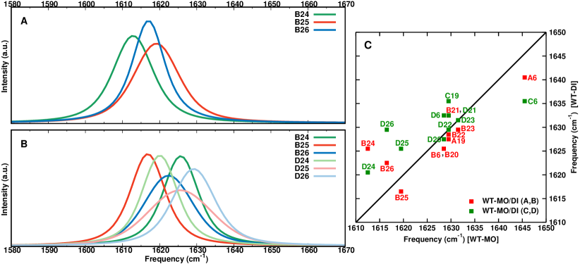
Figure 4: 1D IR spectra for WT monomer (panel A) and dimer (panel B) for residues at the dimerization interface (B24-B26) and (B24-B26, D24-D26), respectively, based on “scan” for frequency calculation. Panel C compares the maximum frequency of the 1D IR spectra for the selected residues (A6, A19, B6, B20-B26, C6, C19, D6, D20-D26) between WT monomer and dimer.

It is also observed that the absolute frequency maximum of the same reporter in the monomer and in the dimer can differ. For example, while the maximum frequency of -CO at position B24 in the monomer is at 1612.5 cm^-1 the maxima for B24 and D24 in the dimer are at 1625.5 cm^-1 and 1620.5 cm^-1. Hence, in addition to a splitting in the dimer spectrum also an overall shift of the frequencies compared with the monomer is found. Again, these effects are largest for the dimerization motif and for residues A/C6, see Figure 4C.

The close agreement of the computed overall spectrum with the experimentally measured one (see above) and the fact that the same computational model was successful in describing the spectroscopy and dynamics of hydrated NMA^{21, 56} provides a meaningful validation of the present approach.

Amide-I Spectroscopy of Wild Type and Mutant Monomers: Mutation at position B24 considerably influences the dimerization behaviour of the hormone.⁵⁶ Hence, the dynamics of the hydrated F24A and F24G monomers was first considered. The infrared lineshapes for residues along the dimerization interface and the same selected -CO probes for the WT monomer are reported in Figure S6. For the two mutant monomers (Figure S6A for F24A and Figure S6B for F24G) the frequency maximum for -CO at position B24 is shifted from 1612.5 cm^-1 (WT) to 1614.5 cm^-1 (F24A) and 1628.5 cm^-1 (F24G), respectively. The amide-I band maxima at positions B25 and B26 show differences for the the F24A mutant but not for F24G and for position A19 the frequency maxima shift to the blue (7 cm^-1) for F24A and to the red (6 cm^-1) for F24G compared to WT. For all other -CO labels in the monomer the differences between F24A and F24G are less than 14 cm^-1.

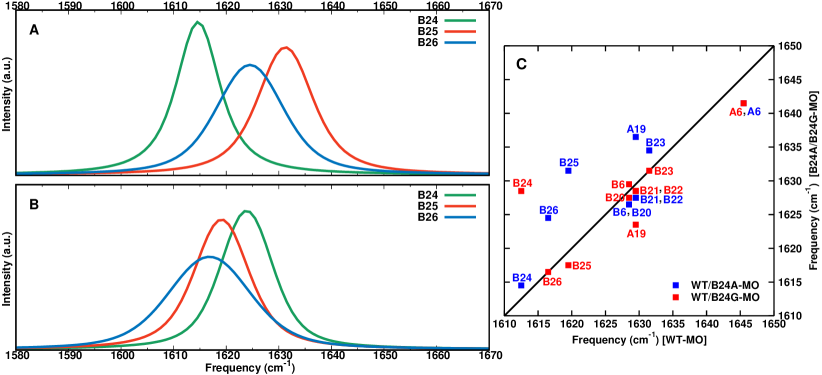
Figure 5: 1D IR spectra for monomeric mutants at position B24. Panels A and B report spectra for F24A (panel A) and F24G (panel B) for residues (B24-B26) at the dimerization interface, based on “scan” for frequency calculations. Panel C compares the maximum frequency of the 1D IR spectra for selected residues (A6, A19, B6, B20-B26) between monomeric WT and mutants F24A and F24G.

A direct comparison of the maxima between the WT and the two mutant monomers is given in Figure 5C for selected -CO probes, as for WT monomer and dimer (see Figure 4). The most pronounced differences in the maximum absorbances occur around the mutation site whereas away from it they are minor, except for -CO at position A19. Interestingly, residue TyrA19 is structurally close to PheB24 (see Figure 1A) which explains the dynamical coupling between the two sites that leads to a shift of $\sim\pm 7$ cm^-1 and is also consistent with recent work on the stability of B24-mutated insulin.⁸

Amide-I Spectroscopy of Wild Type and Mutant Dimers: The peak frequencies for residues at the dimerization interface for the WT and the F24A mutant are reported in Figures 6A and B and directly compared for a larger number of residues, see Figure 6C and S7. As for the monomer, there are specific differences such as for TyrA19, PheB25, and PheD25 which shift by up to 15 cm^-1 between the two systems. For other residues the differences are considerably smaller. For the F24G mutant differences persist, but are in general smaller, see Figure S8. What is found from simulations for both mutants is that residues are not necessarily symetrically affected, in particular for those along the dimerization interface. Also, depending on the modification at position B24 the effects differ and may allow to distinguish between the different insulin variants.

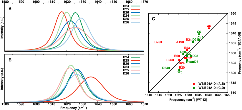
Figure 6: 1D IR spectra for WT (panel A) and the F24A (panel B) dimer for residues at the dimerization interface (B24-B26, D24-D26), based on “scan” for frequency calculation. Panel C compares the maximum frequency of the 1D IR spectra for selected residues (A6, A19, B6, B20-B26, C6, C19, D6, D20-D26) between the WT and F24A mutant dimer.

3.3 Comparison of Amide-I Spectroscopy from Scan, Normal Mode and Map Analyses

The three approaches to determine frequency trajectories considered here (“scan”, “INM”, and “map”) differ considerably in terms of computational expense and the formal approximations in applying them. Scanning along the CO or amide-I normal mode for every snapshot is computationally expensive as it requires for every snapshot to carry out a 1-dimensional scan of the PES, representing it as a RKHS, and solving the nuclear Schrödinger equation. As this needs to be done for $\sim 10^{5}$ snapshots per nanosecond, such an approach does not scale arbitrarily to larger systems and long time scales ($\mu$s or longer). Compared to “scan”, determining instantaneous normal modes is computationally less demanding and the “map” approach is also computationally efficient. In the following, the lineshapes from the frequency trajectory for the WT monomer using the three methods are compared.

Figure 7 reports the 1d lineshapes for all residues of the WT monomer from INM. As for “scan” the maxima of the individual line shapes cover a range between 1625.5 cm^-1 and 1657.5 cm^-1 and the average spectra over all individual lineshapes is centered at 1640.5 cm^-1 with a FWHM of 26 cm^-1, compared with 1630.5 cm^-1 and a FWHM of $\sim 30$ cm^-1 from “scan”, see Figure 3. A direct comparison of the frequency maxima for the WT monomer from “scan” and INM is reported in Figure S9A.

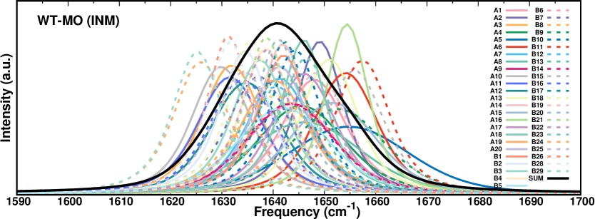
Figure 7: 1D IR spectra for all residues for the WT monomer from INM for the frequency calculations. The black line shows the superposition of all CO spectra compared with other single CO spectrum.

The individual and total lineshapes from using the “map” frequencies are reported in Figure 8. Again, the individual frequency maxima span a range of $\sim 50$ cm^-1 and the FWHM differ for the residues. Contrary to the overall line shape for the monomer from “scan” and “INM”, using the frequency map leads to an infrared spectrum with two peaks. This shape is not consistent with the experimentally observed IR spectrum.^{53, 54} Also, the frequency maxima are somewhat displaced to higher frequencies and do not correlate particularly well with the frequency maxima from “scan” (see Figure S9B). One possibility for these differences may be the fact that for using “map” simulations with constrained -CO are required. Also, the map used in the present work was parametrized with respect to experiments and using a point charge-based force field whereas the simulations in the present work used multipoles.

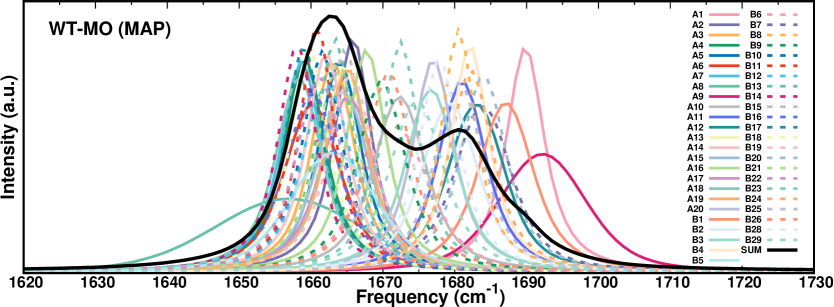
Figure 8: 1D IR spectra for all residues in WT monomer based on “map” for the frequency calculation. The labels for the individual line shapes are given in the panel and the overall sum is the solid black line. The line shapes are determined from 1 ns simulations and the snapshots analyzed are separated by 10 fs.

Next, the lineshapes for the residues involved in the dimerization interface and the selection of other residues already considered until now are analyzed for WT monomer and dimer for INM and “map”, see Figures 9, 10, S10, and S11. When using INM it is again found that for the residues at the dimerization interface the location of the frequency maxima in the two monomers differ and also change compared with the isolated monomer (see Figure 9C). These effects are not only observed for residues at the interface but also away from it. Splitting for B/D24, B/D25, and B/D26 are comparable or larger than with “scan” and blue/red shifts are consistent for the two methods.

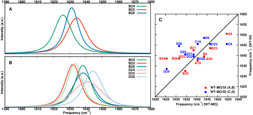
Figure 9: 1D IR spectra from INM for residues (B24-B26) and (B24-B26, D24-D26) at the dimerization interface for WT monomer (panel A) and WT dimer (panel B). Panel C compares the maximum frequency of the 1D IR spectra for the residues (A6, A19, B6, B20-B26, C6, C19, D6, D20-D26) between WT monomer and dimer.

For the analysis using “map” in Figure 10 it is important to note that they do not use the same structures for analysis as for “scan” and INM because the -CO bond lengths were constrained. As for the other two methods the frequency maxima for B24 to B26 do not coincide for the monomer (Figure 10A) and the -CO labels in the two monomers have their maxima at different frequencies in the dimer (Figure 10B). However, the actual frequency maxima between the three methods differ. The effect of constrained and flexible -CO in the MD simulations is reported in Figure S12. For a comparison of the maximum frequencies for the three methods for B24 to B26 and D24 to D26 for direct numerical comparison, see Table 1. Figure S13 reports a comparison of the map used here and an alternative parametrization.¹⁶ Consistent with earlier work that compared the performance of different maps,⁵⁷ it is found that the two correlate quite well (within a few cm^-1) except for residue B20 for which they differ by $\sim 25$ cm^-1. It is noteworthy that for both, scanning along the [CONH] normal mode (Figure S1) and for using “map” (Figure S9) compared with scanning along the CO mode, the frequency maxima are shifted towards the blue, in accord with experiment (frequency maximum $\sim 1650$ cm^-1).^{53, 54}

Residue	Scan	INM	Map
B24	1612.5	1625.5	1682.5
B25	1619.5	1634.5	1680.5
B26	1616.5	1631.5	1670.5

Table 1: Position of the frequency maxima of the 1D IR spectra for WT monomer using the three different approaches (“scan”, “INM”, and “map”). For “scan” and INM the CO probes are flexible while for ”map” the structures were those from a simulation with constrained CO bond length.

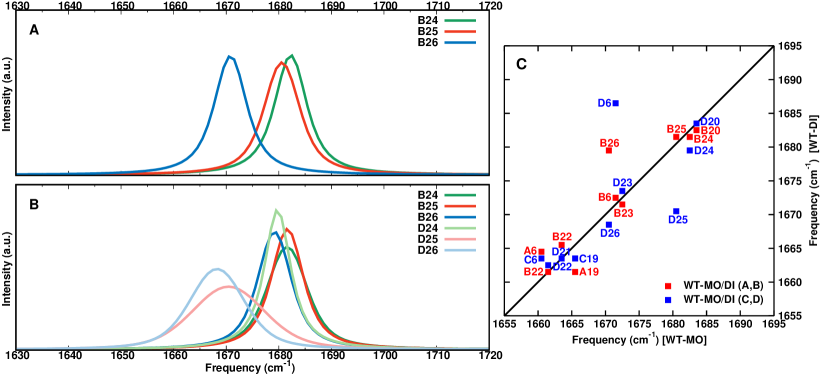
Figure 10: 1D IR spectra from ”map” for residues (B24-B26) and (B24-B26, D24-D26) at the dimerization interface for WT monomer (panel A) and WT dimer (panel B). Panel C compares the maximum frequency of the 1D IR spectra for the residues (A6, A19, B6, B20-B26, C6, C19, D6, D20-D26) between WT monomer and dimer. The CO bond length is constrained in the MD simulations.

Using “map” the labels at B/D25 and B/D26 show splittings comparable to those from “scan” and INM whereas for B/D24 the splitting is only 1 to 3 cm^-1 which is considerably smaller than for the two other methods. Nevertheless, the results from “map” also indicate that the spectroscopic signatures of the residues at the dimerization interface are not identical and differ from the monomer whereas for the other residues considered the differences between monomer and dimer and the two monomers within the dimer are smaller.

In summary, all three methods agree in that a) the individual labels have their frequency maxima at different frequencies and b) in going from the WT monomer to the dimer the IR spectra of the labels involved in dimerization split and shift. The magnitude of the splitting and shifting differs between the methods which is not surprising given their very different methodologies. For the two mutants F24A and F24G the IR lineshapes using “scan” were determined for the residues involved in the dimerization interface and a selection of other residues, see Figure 1A. Compared with the WT monomer and dimer, characteristic shifts were found.

3.4 Frequency Fluctuation Correlation Functions

The frequency fluctuation correlation functions that can be computed from the frequency time series contain valuable information about the dynamics around a particular site considered, here the -CO groups of every residue. Specifically, FFCFs were analyzed for labels along the dimerization interface, for WT and the two mutant monomers and dimers, from using frequencies determined from “scan” and INM. Before discussing the FFCFs their convergence with simulation time is considered as it has been observed that an extensive amount of data is required.²²

For this, the first 1 ns and the entire 5 ns run for WT insulin monomer was analyzed using “scan”. For the 1 ns simulation snapshots every 10 fs and every 2 fs were analyzed (see Figure S14 top and middle row) and every 10 fs for the 5 ns simulations (Figure S14 bottom row). The computational resources required for such an analysis are considerable. Using 8 processors, the analysis of the 1 ns simulation for $10^{5}$ snapshots (saved every 10 fs) takes 400 hours for a single spectroscopic probe. Figure S14 shows that except for one feature at $\sim 3$ ps for residue B26 the FFCFs from the 1 ns simulation with saving every 10 fs and every 2 fs are very similar. On the contrary, using snapshots from the 5 ns simulation leads to reducing the fluctuations in the FFCFs and determinants such as the static component (the value at a correlation time of 4 ps) are higher from the longer simulation. A quantitative comparison for the time scales, amplitudes and static component (see Eq. 5) is provided in Figure S15 and in Table S2. The amplitudes and short decay times of all fits are within a few percent. The picosecond time scale ($\tau_{2}$) can differ by up to 30 % (B26) and the offset $\Delta_{0}$ can differ by a factor of two or more. To balance computational expense and quality of data, the remaining analysis was carried out with data from the 1 ns simulation with snapshots recorded every 10 fs.

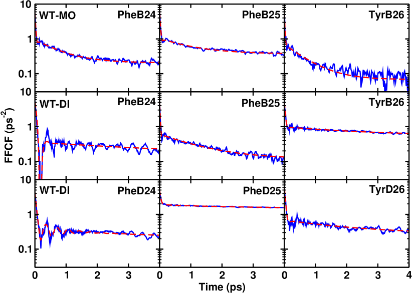
Figure 11: Comparison of the FFCFs for WT monomer and dimer for residues B24 to B26 at the dimerization interface. The frequencies are based on “scan” and snapshots from the 1 ns simulation, saved every 10 fs were analyzed.

The FFCFs for B24 to B26 of the insulin monomer and the two monomers within the dimer are reported in Figure 11 together with the fits to Eq. 5. For the three labels from the monomer simulations the FFCFs differ in the longest decay time and the offset $\Delta_{0}$. As for the infrared spectra, the three -CO labels exhibit different environmental dynamics. When compared with the two monomers in the insulin dimer these differences are even more pronounced. In general, all decay times increase to between 1 ps and $\sim 13$ ps and the offset can be up to 5 times larger than for the monomer. This is owed to the considerably restrained dynamics of the residues at the dimerization interface compared with the free monomer.

	$a_{1}$	$\gamma$	$\tau_{1}$	$a_{2}$	$\tau_{2}$	$\Delta_{0}$	$a_{3}$	$\tau_{3}$
WT monomer
B24	4.64	25.44	0.025	0.75	0.74	0.21
B25	4.94	22.19	0.028	0.66	0.98	0.37
B26	4.97	21.82	0.019	0.62	0.62	0.07
WT dimer M1
B24	4.80	14.50	0.080	0.23	4.72	0.13
B25	3.92	27.74	0.023	0.49	1.15	0.12
B26	4.12	16.36	0.038	0.44	2.51	0.55
WT dimer M2
D24	0.30	17.59	0.56	3.68	0.039	0.18	0.19	4.08
D25	3.17		0.033	0.41	2.32	1.50
D26	5.32	13.49	0.040	0.42	2.10	0.27
F24A monomer
B24	4.94	29.51	0.020	0.51	0.61	0.07
B25	4.37	13.45	0.020	0.64	0.79	0.21
B26	4.11	25.05	0.027	0.63	1.38	0.45
F24A dimer M1
B24	4.90	14.61	0.046	0.33	1.68	0.41
B25	3.19		0.028	0.62	1.81	1.08
B26	2.15		0.040	0.34	1.89	0.48
F24A dimer M2
D24	1.27		0.043	0.31	1.17	0.36
D25	1.39		0.031	0.32	1.10	0.51
D26	4.91	13.72	0.039	0.60	1.40	0.63
F24G monomer
B24	4.72	29.74	0.032	0.43	1.24	0.26
B25	4.57	16.46	0.019	0.58	0.81	0.24
B26	4.60	25.73	0.022	0.59	0.54	0.04	0.51	7.89
F24G dimer M1
B24	1.42		0.028	0.21	1.02	0.37
B25	3.70		0.018	0.48	1.18	0.24
B26	3.87		0.029	0.68	1.90	0.88
F24G dimer M2
D24	2.50	38.76	0.016	0.30	1.29	0.17
D25	1.53		0.030	0.25	1.70	0.65
D26	3.94	5.32	0.042	0.27	2.14	0.23

Table 2: Parameters from fitting the FFCF to Eq. 5 for frequencies from “scan” for the selected residues (B24-B26 and D24-D26). The amplitudes $a_{1}$ to $a_{3}$ in ps^-2, the decay times $\tau_{1}$ to $\tau_{3}$ in ps, the parameter $\gamma$ in ps^-1, and the offset $\Delta_{0}$ in ps^-2. For residues D24 in monomer M2 from the WT dimer and B26 in the F24G monomer the third time scale is required for a good fit.

Comparing the two monomer mutants with the WT it is found that the picosecond component is comparable whereas $\Delta_{0}$ is similar (for F24A) or somewhat larger (for F24G), see Table 2. When moving to the mutant dimers, the differences with their monomeric counterparts are considerably smaller than for the WT system. This is likely to be related to a weakening of the F24A and F24G dimers which also allows water to penetrate more or less deeply into the dimer interface.⁸ Overall, the dynamics still is slowed down in the mutant dimers by up to a factor of two compared with the mutant monomer but the effects are considerably less pronounced than for the WT systems.

FFCFs were also determined from frequency trajectories determined from the INMs for the three residues at the dimerization interface, see Table S3. The findings are similar to those from analyzing frequencies from “scan” whereas the actual numerical values for amplitudes, decay times and offset differ somewhat.

4 Conclusion

The present work demonstrates that WT insulin monomer and dimer and mutant monomers and mutant dimers lead to different spectroscopic and dynamical signatures for residues along the dimerization interface. This is found - to different extent - for all three approaches used for computing the frequency trajectory (“scan”, INM, “map”) and suggests that the overall findings do not depend strongly on the way how these frequencies are determined. The center frequency and FWHM for insulin monomer are in qualitative (scan along CO INM) or even quantitative (scan along [CONH] INM) agreement with experiment which, together with earlier investigations of the spectroscopy and dynamics of and around NMA,^{21, 34, 47} provide a validation of the computational model. It is noteworthy that using one single parametrization for the -CO stretch and the multipoles on the [CONH] moiety of the peptide bond the experimentally observed FWHM for the protein is correctly described.

The fact that the stability differences between WT and mutant (here at position B24)⁸ insulin dimer are also reflected in the spectroscopy and dynamics of WT and mutant insulin monomers and dimers suggests that spectroscopic investigations can be used to provide information about the association thermodynamics. This follows earlier suggestions for characterizing protein-ligand binding¹¹ which are supported by atomistic simulations.¹² For insulin this is particularly relevant because except for the WT dimer direct thermodynamic information about its stability appears to be missing. Replacing a thermodynamic approach by a spectroscopic characterization is an attractive alternative. The present work suggests that by combining quantitative simulations with modern experiments is a potentially useful way to obtain pharmacologically relevant information such as the strength of the modified insulin dimers.

Supporting Information

The supporting information reports further comparison of the infrared spectra for WT and mutant insulin monomer and dimer. Additional validation of the FFCF and comparisons of two different spectroscopic maps are provided as well.

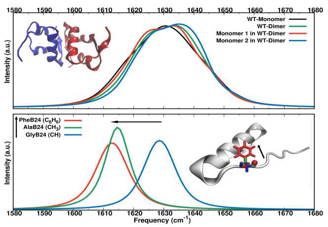
labelformat=empty

Figure 12: TOC Graphic

References

- Strazza et al. 1985 Strazza, S.; Hunter, R.; Walker, E.; Darnall, D. W. The thermodynamics of bovine and porcine insulin and proinsulin association determined by concentration difference spectroscopy. Archives of Biochemistry and Biophysics 1985, 238, 30–42
- Tidor and Karplus 1994 Tidor, B.; Karplus, M. The contribution of vibrational entropy to molecular association: the dimerization of insulin. J. Mol. Biol. 1994, 238, 405–414
- Zoete et al. 2005 Zoete, V.; Meuwly, M.; Karplus, M. Study of the insulin dimerization: Binding free energy calculations and per-residue free energy decomposition. Proteins: Structure, Function, and Bioinformatics 2005, 61, 79–93
- Baker et al. 1988 Baker, E.; Blundell, T.; Cutfield, J.; Cutfield, S.; Dodson, E.; Dodson, G.; Hodgkin, D.; Hubbard, R.; Isaacs, N.; Reynolds, C. The structure of 2Zn pig insulin crystals at 1.5 Å resolution. Phil. Trans. R. Soc. Lond. B Biol. 1988, 319, 369–456
- Zhang and Tokmakoff 2020 Zhang, X.-X.; Tokmakoff, A. Revealing the Dynamical Role of Co-solvents in the Coupled Folding and Dimerization of Insulin. J. Phys. Chem. Lett. 2020, 11, 4353–4358
- Banerjee et al. 2018 Banerjee, P.; Mondal, S.; Bagchi, B. Insulin dimer dissociation in aqueous solution: A computational study of free energy landscape and evolving microscopic structure along the reaction pathway. J. Chem. Phys. 2018, 149
- Antoszewski et al. 2020 Antoszewski, A.; Feng, C.-J.; Vani, B. P.; Thiede, E. H.; Hong, L.; Weare, J.; Tokmakoff, A.; Dinner, A. R. Insulin Dissociates by Diverse Mechanisms of Coupled Unfolding and Unbinding. J. Phys. Chem. B 2020, 124, 5571–5587
- Raghunathan et al. 2018 Raghunathan, S.; El Hage, K.; Desmond, J. L.; Zhang, L.; Meuwly, M. The Role of Water in the Stability of Wild-type and Mutant Insulin Dimers. J. Phys. Chem. B 2018, 122, 7038–7048
- Wang et al. 2019 Wang, P.; Wang, X.; Liu, L.; Zhao, H.; Qi, W.; He, M. The Hydration Shell of Monomeric and Dimeric Insulin Studied by Terahertz Time-Domain Spectroscopy. Biophys. J. 2019, 117, 533–541
- Banerjee and Bagchi 2020 Banerjee, P.; Bagchi, B. Dynamical control by water at a molecular level in protein dimer association and dissociation. Proc. Natl. Acad. Sci. 2020, 117, 2302–2308
- Suydam et al. 2006 Suydam, I. T.; Snow, C. D.; Pande, V. S.; Boxer, S. G. Electric Fields at the Active Site of an Enzyme : Direct Comparison of Experiment with Theory. Science 2006, 313, 200–204
- Mondal and Meuwly 2017 Mondal, P.; Meuwly, M. Vibrational Stark Spectroscopy for Assessing Ligand-Binding Strengths in a Protein. Phys. Chem. Chem. Phys. 2017, 19, 16131–16143
- Bereau et al. 2013 Bereau, T.; Kramer, C.; Meuwly, M. Leveraging Symmetries of Static Atomic Multipole Electrostatics in Molecular Dynamics Simulations. J. Chem. Theo. Comp. 2013, 9, 5450–5459
- Plattner and Meuwly 2008 Plattner, N.; Meuwly, M. The Role of Higher CO-Multipole Moments in Understanding the Dynamics of Photodissociated Carbonmonoxide in Myoglobin. Biophys. J. 2008, 94, 2505–2515
- Nutt and Meuwly 2003 Nutt, D.; Meuwly, M. Theoretical investigation of infrared spectra and pocket dynamics of photodissociated carbonmonoxy myoglobin. Biophys. J. 2003, 85, 3612–3623
- Wang et al. 2011 Wang, L.; Middleton, C. T.; Zanni, M. T.; Skinner, J. L. Development and Validation of Transferable Amide I Vibrational Frequency Maps for Peptides. J. Phys. Chem. B 2011, 115, 3713–3724
- Jansen et al. 2006 Jansen, T. l. C.; Dijkstra, A. G.; Watson, T. M.; Hirst, J. D.; Knoester, J. Modeling the amide I bands of small peptides. J. Chem. Phys. 2006, 125
- Jansen et al. 2012 Jansen, T. l. C.; Dijkstra, A. G.; Watson, T. M.; Hirst, J. D.; Knoester, J. Modeling the amide I bands of small peptides (vol 125, 044312, 2006). J. Chem. Phys. 2012, 136
- Reppert and Tokmakoff 2013 Reppert, M.; Tokmakoff, A. Electrostatic frequency shifts in amide I vibrational spectra: Direct parameterization against experiment. J. Chem. Phys. 2013, 138
- Lee et al. 2013 Lee, M. W.; Carr, J. K.; Göllner, M.; Hamm, P.; Meuwly, M. 2D IR Spectra of Cyanide in Water Investigated by Molecular Dynamics Simulations. J. Chem. Phys. 2013, 139, 054506
- Cazade et al. 2014 Cazade, P.-A.; Bereau, T.; Meuwly, M. Computational Two-Dimensional Infrared Spectroscopy without Maps: N-Methylacetamide in Water. J. Phys. Chem. B 2014, 118, 8135–8147
- Salehi et al. 2019 Salehi, S. M.; Koner, D.; Meuwly, M. Vibrational Spectroscopy of N in the Gas and Condensed Phase. J. Phys. Chem. B 2019, 123, 3282–3290
- Hua et al. 1991 Hua, Q. X.; Shoelson, S. E.; Kochoyan, M.; Weiss, M. A. Receptor binding redefined by a structural switch in a mutant human insulin. Nature 1991, 354, 238–241
- Shoelson et al. 1983 Shoelson, S.; Fickova, M.; Haneda, M.; Nahum, A.; Musso, G.; Kaiser, E.; Rubenstein, A.; Tager, H. Identification of a mutant human insulin predicted to contain a serine-for-phenylalanine substitution. Proc. Natl. Acad. Sci. 1983, 80, 7390–7394
- Haneda et al. 1985 Haneda, M.; Kobayashi, M.; Maegawa, H.; Watanabe, N.; Takata, Y.; Ishibashi, O.; Shigeta, Y.; Inouye, K. Decreased biologic activity and degradation of human [SerB24]-insulin, a second mutant insulin. Diabetes 1985, 34, 568–573
- Tager et al. 1980 Tager, H.; Thomas, N.; Assoian, R.; Rubenstein, A.; Saekow, M.; Olefsky, J.; Kaiser, E. Semisynthesis and biological activity of porcine [LeuB24] insulin and [LeuB25] insulin. Proc. Natl. Acad. Sci. 1980, 77, 3181–3185
- Žáková et al. 2013 Žáková, L.; Kletvíková, E.; Veverka, V.; Lepšík, M.; Watson, C. J.; Turkenburg, J. P.; Jiráček, J.; Brzozowski, A. M. Structural integrity of the B24 site in human insulin is important for hormone functionality. J. Biol. Chem. 2013, 288, 10230–10240
- Chen et al. 2000 Chen, H.; Shi, M.; Guo, Z.-Y.; Tang, Y.-H.; Qiao, Z.-S.; Liang, Z.-H.; Feng, Y.-M. Four new monomeric insulins obtained by alanine scanning the dimer-forming surface of the insulin molecule. Protein Engineering 2000, 13, 779–782
- DeFelippis et al. 2001 DeFelippis, M. R.; Chance, R. E.; Frank, B. H. Insulin self-association and the relationship to pharmacokinetics and pharmacodynamics. Critical Reviews in Therapeutic Drug Carrier Systems 2001, 18
- Brooks et al. 2009 Brooks, B. R.; Brooks III, C. L.; MacKerell Jr., A. D.; Nilsson, L.; Petrella, R. J.; Roux, B.; Won, Y.; Archontis, G.; Bartels, C.; Boresch, S. et al. CHARMM: The Biomolecular Simulation Program. J. Comp. Chem. 2009, 30, 1545–1614
- J. A. MacKerell 1998 J. A. MacKerell, et. al.. All-Atom Empirical Potential for Molecular Modeling and Dynamics Studies of Proteins. J. Phys. Chem. B 1998, 102, 3586–3616
- Mackerell et al. 2004 Mackerell, A.; Feig, M.; Brooks, C. Extending the treatment of backbone energetics in protein force fields: Limitations of gas-phase quantum mechanics in reproducing protein conformational distributions in molecular dynamics simulations. J. Comp. Chem. 2004, 25, 1400–1415
- MacKerell et al. 2004 MacKerell, A.; Feig, M.; Brooks, C. Improved treatment of the protein backbone in empirical force fields. J. Am. Chem. Soc. 2004, 126, 698–699
- Cazade et al. 2015 Cazade, P.-A.; Hedin, F.; Xu, Z.-H.; Meuwly, M. Vibrational Relaxation and Energy Migration of N-Methylacetamide in Water: The Role of Non bonded Interactions. J. Phys. Chem. B 2015, 119, 3112–3122
- Jorgensen et al. 1983 Jorgensen, W. L.; Chandrasekhar, J.; Madura, J. D.; Impey, R. W.; Klein, M. L. Comparison of Simple Potential Functions for Simulating Liquid Water. J. Chem. Phys. 1983, 79, 926–935
- Kramer et al. 2012 Kramer, C.; Gedeck, P.; Meuwly, M. Atomic Multipoles: Electrostatic Potential Fit, Local Reference Axis Systems and Conformational Dependence. J. Comp. Chem. 2012, 33, 1673–1688
- Swope et al. 1982 Swope, W. C.; Andersen, H. C.; Berens, P. H.; Wilson, K. R. A Computer Simulation Method for the Calculation of Equilibrium Constants for the Formation of Physical Clusters of Molecules: Application to Small Water Clusters. J. Chem. Phys. 1982, 76, 637–649
- Nosé 1984 Nosé, S. A Unified Formulation o the Constant Temperature Molecular-Dynamics Methods. J. Chem. Phys. 1984, 81, 511–519
- Hoover 1985 Hoover, W. G. Canonical Dynamics: Equilibrium Phase-Space Distributions. Phys. Rev. A 1985, 31, 1695–1697
- Andersen 1980 Andersen, H. C. Molecular Dynamics Simulations at Constant Pressure and/or Temperature. J. Chem. Phys. 1980, 72, 2384–2393
- Nosé and Klein 1983 Nosé, S.; Klein, M. L. Constant Pressure Molecular Dynamics for Molecular Systems. Mol. Phys. 1983, 50, 1055–1076
- Hairer et al. 2003 Hairer, E.; Lubich, C.; Wanner, G. Geometric Numerical Integration Illustrated by the Störmer/Verlet Method. Acta Numerica 2003, 12, 399–450
- Gunsteren and Berendsen 1997 Gunsteren, W. V.; Berendsen, H. Algorithms for Macromolecular Dynamics and Constraint Dynamics. Mol. Phys. 1997, 34, 1311–1327
- Steinbach and Brooks 1994 Steinbach, P. J.; Brooks, B. R. New Spherical-Cutoff Methods for Long-Range Forces in Macromolecular Simulation. J. Comp. Chem. 1994, 15, 667–683
- Darden et al. 1993 Darden, T.; York, D.; Pedersen, L. Particle Mesh Ewald: An Nlog(N) Method for Ewald Sums in Large Systems. J. Chem. Phys. 1993, 98, 10089–10092
- Colbert and Miller 1992 Colbert, D. T.; Miller, W. H. A novel discrete variable representation for quantum mechanic al reactive scattering via the S-matrix method. J. Chem. Phys. 1992, 96, 1982–1991
- Koner et al. 2020 Koner, D.; Salehi, S. M.; Mondal, P.; Meuwly, M. Non-conventional force fields for applications in spectroscopy and chemical reaction dynamics. J. Chem. Phys. 2020, 153, 010901
- Hamm and Zanni 2011 Hamm, P.; Zanni, M. Concepts and Methods of 2D Infrared Spectroscopy; Cambridge University Press: New York, 2011
- Moller et al. 2004 Moller, K.; Rey, R.; Hynes, J. Hydrogen Bond Dynamics in Water and Ultrafast Infrared Spectroscopy: A Theoretical Study. J. Phys. Chem. A 2004, 108, 1275–1289
- Li et al. 2006 Li, S.; Schmidt, J. R.; Piryatinski, A.; Lawrence, C. P.; Skinner, J. L. Vibrational Spectral Diffusion of Azide in Water. J. Phys. Chem. B 2006, 110, 18933–18938
- Virtanen et al. 2020 Virtanen, P.; Gommers, R.; Oliphant, T. E.; Haberland, M.; Reddy, T.; Cournapeau, D.; Burovski, E.; Peterson, P.; Weckesser, W.; Bright, J. et al. SciPy 1.0: Fundamental Algorithms for Scientific Computing in Python. Nature Methods 2020, 17, 261–272
- Zoete et al. 2004 Zoete, V.; Meuwly, M.; Karplus, M. A comparison of the dynamic behavior of monomeric and dimeric insulin shows structural rearrangements in the active monomer. J. Mol. Biol. 2004, 342, 913–929
- Dhayalan et al. 2016 Dhayalan, B.; Fitzpatrick, A.; Mandal, K.; Whittaker, J.; Weiss, M. A.; Tokmakoff, A.; Kent, S. B. H. Efficient Total Chemical Synthesis of C-13=O-18 Isotopomers of Human Insulin for Isotope-Edited FTIR. Chem. Bio. Chem. 2016, 17, 415–420
- Zhang et al. 2016 Zhang, X.-X.; Jones, K. C.; Fitzpatrick, A.; Peng, C. S.; Feng, C.-J.; Baiz, C. R.; Tokmakoff, A. Studying Protein-Protein Binding through T-Jump Induced Dissociation: Transient 2D IR Spectroscopy of Insulin Dimer. J. Phys. Chem. B 2016, 120, 5134–5145
- Falconi et al. 2001 Falconi, M.; Cambria, M.; Cambria, A.; Desideri, A. Structure and stability of the insulin dimer investigated by molecular dynamics simulation. J. Biomol. Struc. Dyn. 2001, 18, 761–772
- Desmond et al. 2019 Desmond, J. L.; Koner, D.; Meuwly, M. Probing the Differential Dynamics of the Monomeric and Dimeric Insulin from Amide-I IR Spectroscopy. J. Phys. Chem. B 2019, 123, 6588–6598
- Reppert et al. 2015 Reppert, M.; Roy, A. R.; Tokmakoff, A. Isotope-enriched protein standards for computational amide I spectroscopy. J. Chem. Phys. 2015, 142
\captionsetup