On System-Wide Safety Staffing of Large-Scale
Parallel Server Networks System-Wide Safety Staffing of Parallel Server Networks H. Hmedi, A. Arapostathis, and G. Pang

Hassan Hmedi, Ari Arapostathis Department of Electrical and Computer Engineering, The University of Texas at Austin,
2501 Speedway, EER 7.824, Austin, TX  78712, [hmedi,ari]@utexas.edu Guodong Pang The Harold and Inge Marcus Dept. of Industrial and Manufacturing Eng., College of Engineering,
Pennsylvania State University, University Park, PA  16802, gup3@psu.edu

We introduce a “system-wide safety staffing” (SWSS) parameter for multiclass multi-pool networks of any tree topology, Markovian or non-Markovian, in the Halfin–Whitt regime. This parameter can be regarded as the optimal reallocation of the capacity fluctuations (positive or negative) of order $\sqrt{n}$ when each server pool employs a square-root staffing rule. We provide an explicit form of the SWSS as a function of the system parameters, which is derived using a graph theoretic approach based on Gaussian elimination.

For Markovian networks, we give an equivalent characterization of the SWSS parameter via the drift parameters of the limiting diffusion. We show that if the SWSS parameter is negative, the limiting diffusion and the diffusion-scaled queueing processes are transient under any Markov control, and cannot have a stationary distribution when this parameter is zero. If it is positive, we show that the diffusion-scaled queueing processes are uniformly stabilizable, that is, there exists a scheduling policy under which the stationary distributions of the controlled processes are tight over the size of the network. In addition, there exists a control under which the limiting controlled diffusion is exponentially ergodic. Thus we have identified a necessary and sufficient condition for the uniform stabilizability of such networks in the Halfin-Whitt regime.

We use a constant control resulting from the leaf elimination algorithm to stabilize the limiting controlled diffusion, while a family of Markov scheduling policies which are easy to compute are used to stabilize the diffusion-scaled processes. Finally, we show that under these controls the processes are exponentially ergodic and the stationary distributions have exponential tails.

90B22, 60K25, 49L20, 90B36

parallel server networks, Halfin–Whitt regime, system-wide safety staffing, uniform stabilizability

1 Introduction

In recent years, parallel server networks have been a subject of intense study due to their use in modeling a variety of systems including telecommunications, patient flows, service and data centers, etc. The stability analysis of such systems is quite challenging because of their complexity. In this paper, we focus on studying the safety staffing and stability of such networks of any tree topology in the Halfin–Whitt regime (or Quality–and–Efficiency–Driven (QED) regime) in which the number of servers and the arrival rates grow with the system scale while fixing the service rates in a way that the system becomes critically loaded (Halfin and Whitt 1981, Whitt 1992, Borst et al. 2004).

When there is at least one class of jobs having a positive abandonment rate, it is well known that there exists a scheduling policy under which the stationary distributions of the controlled diffusion-scaled queueing processes are tight (uniformly stable in the size of the network) (Arapostathis and Pang 2016, 2018, 2019). On the other hand, for networks with no abandonment, such results have only been established for particular topologies. For the Markovian ‘V’ network, it is shown in Gamarnik and Stolyar (2012) and Arapostathis et al. (2020a) (the latter considers renewal arrivals, and the limiting diffusion) that, if the server pool has $\sqrt{n}$ safety staffing, then the stationary distributions of the controlled diffusion-scaled queueing processes under work-conserving stationary Markov scheduling policy are tight. This is a very strong stability property since it is independent of the system order or any particular work-conserving policy. We say such networks are uniformly stable. For the ‘N’ network, Stolyar (2015) has shown that, with $\sqrt{n}$ safety staffing in one server pool, the stationary distributions of the controlled diffusion-scaled queueing processes are tight under a static priority scheduling policy. For a large class of Markovian networks, which includes those with a single nonleaf server pool, like the ‘N’ and ‘M’ models, and networks with class-dependent service rates, a quantity referred to as $\sqrt{n}$ spare capacity is identified in Hmedi et al. (2019), and it is shown that when it is positive, the stationary distributions of the controlled diffusion-scaled queueing processes are tight over the class of system-wide work-conserving policies. On the other hand, in Stolyar and Yudovina (2013), under a natural load balancing policy referred to as “Longest-Queue Freest-Server”, it is shown that the stationary distributions of the controlled diffusion-scaled queueing processes may not be tight for a network of arbitrary tree topology, but they are tight for the class of networks with pool-dependent service rates.

In Systems Theory, the existence of a control that renders a system stable, is usually referred to as stabilizability. Adopting the same terminology, we say that a network is uniformly stabilizable if there exists some Markov scheduling policy under which the diffusion-scaled state process is positive recurrent and the invariant distributions (over all sufficiently large orders of the network) are tight. The following question is then raised. For parallel–server networks with an arbitrary tree topology and no abandonment, is there a sharp criterion to determine if a network is uniformly stabilizable? We are seeking a quantity which if positive, the network is uniformly stabilizable, and if negative, then the state process is transient under any Markov scheduling policy. In this paper we provide an affirmative answer to the previous question through a parameter called system-wide safety staffing (SWSS), and which can be easily computed from the system data. Thus, the main result of the paper states that there exists a scheduling policy under which the stationary distributions of the controlled diffusion-scaled queueing processes are tight if and only if the network has positive SWSS, meaning that the SWSS parameter is positive. As expected, for ‘V’ and ‘N’ networks, the SWSS parameter is the same as the $\sqrt{n}$ safety staffing discussed in the preceding paragraph.

For a better understanding of the SWSS parameter, it is worth recalling the complete resource pooling (CRP) condition and the demand and supply rates in the scales of order ${\mathscr{O}}(n)$ and ${\mathscr{O}}(\sqrt{n})$ in the Halfin–Whitt regime. The CRP condition requires that given a demand in the scale of order ${\mathscr{O}}(n)$, each server pool has a suitable number of ${\mathscr{O}}(n)$ of servers so that there exists a unique allocation of the capacity in each server pool to meet the demand of every class it can serve. This of course determines the fluid limit. More precisely, suppose that the arrival rates of the $n^{\mathrm{t}h}$ system are $\lambda^{n}_{i}=n\lambda_{i}$, where $i$ refers to the $i^{\mathrm{th}}$ class of jobs, and the $\lambda_{i}$’s are fixed positive numbers. Then the steady state allocations of servers in each pool are given by the linear program Eq. LP in Section 2. If the sever pools have an excess ${\mathscr{O}}(\sqrt{n})$ of servers from what is required to meet this state allocation, then one can of course expect that the system can be rendered stable by a suitable choice of a scheduling policy. On the other hand, if some server pools are deficient, that is, they are understaffed by an amount of ${\mathscr{O}}(\sqrt{n})$ servers, then the answer is not at all clear. Thus, an important contribution of this paper, is that it quantifies the ‘value’ of a server in a given pool. It can answer the question of whether moving a given number of servers from one pool to another has a positive impact on system stability (see Remark 3.4). Moreover, the arrival rates in this paper also have a $\sqrt{n}$ component, that is, $\lambda^{n}_{i}\approx n\lambda_{i}+\hat{\lambda}_{i}\sqrt{n}$, and as a result the SWSS parameter depends on the deviation of the arrival rates from the nominal values $n\lambda_{i}$.

The SWSS parameter $\vartheta_{p}$ is obtained via the linear program Eq. LP^′, whereas a similar program in Eq. $\mathsf{LP}_{n}^{\prime}$ determines a parameter $\vartheta_{p}^{n}$ for the $n^{\mathrm{th}}$ system (see Definition 2.1). The asymptotic behavior of the system parameters in the Halfin–Whitt regime (see Eqs. 1 and 2) implies that $\vartheta_{p}^{n}$ tends to $\vartheta_{p}$ as $n\to\infty$. It is asserted in Theorem 2.4 that if $\vartheta_{p}$ ($\vartheta_{p}^{n}$) are negative, then the limiting diffusion ($n^{\mathrm{th}}$-system) are transient under any Markov control. On the other hand, if $\vartheta_{p}>0$, then the limiting diffusion is exponentially ergodic under some Markov control, and the $n^{\mathrm{th}}$-systems are uniformly stabilizable for all large enough $n$. Thus, the SWSS is an important and nontrivial extension of the familiar square-root safety staffing parameter for single-class multi-server queues (Halfin and Whitt 1981, Whitt 1992).

A major contribution of this paper is a closed form expression for the SWSS as a function of the system parameters. Deriving this relies on solving the optimization problem in Eq. LP^′ via a simple Gaussian elimination of variables. It is important to emphasize that the definition of the SWSS and its functional form apply to multiclass multi-pool networks of $G/G/N$ queues, regardless if they are Markovian or non-Markovian, since only the arrival and service rates play a role in this formulation.

The results carry over to the limiting diffusion of the Markovian networks in an interesting manner. We present in Section 4 a useful formula which allows us to compute the SWSS as a function the drift parameters of the limiting diffusion. This relies on the explicit expression of the drift derived from using the iterative leaf elimination algorithm developed in Arapostathis and Pang (2016), whose important properties are summarized in Proposition 4.4. Moreover, we also provide an explicit matching expression (except an additional term indicating the violation of joint work conservation in the $n^{\rm th}$ system) for the infinitesimal drift of the diffusion-scaled Markovian queueing processes and some key properties of the main components in the expression in Proposition 4.2. These properties of the drift expressions for both the diffusion-scaled processes and the limiting diffusions play a crucial rule for the stability analysis.

In Section 5 we show that the positivity of the SWSS is necessary for stabilizability. In particular, we show in Theorem 5.3 that if $\vartheta_{p}<0$, then the limiting diffusion process $\{X_{t}\}_{t\geq 0}$ is transient under any Markov control, and if $\vartheta_{p}=0$, then it cannot be positive recurrent. Also, in Theorem 5.6, we show that the exact analogous statement (with the parameter $\vartheta^{n}_{p}$) applies to the state process of the $n^{\mathrm{th}}$ system. These results extend Hmedi et al. (2019, Propositions 3.1 and 3.2) to networks with general tree topologies. The proof of the above mentioned results relies on an important structural property of the drift of the limiting diffusion stated in Lemma 5.1 (see also Corollary 5.5 for the drift of the diffusion-scaled state process).

In Section 6, we exhibit a class of stabilizing controls for the diffusion-scaled queueing processes and the limiting diffusion when the SWSS is positive. In order to accomplish this, we introduce an appropriate “centering” for the diffusion-scaled processes, which allows us to establish Foster–Lyapunov equations. The stabilizing controls we use, consist of the family of balanced saturation policies (BSPs) introduced in Arapostathis and Pang (2019), where exponential ergodicity has been shown for networks with at least one positive abandonment rates. On the other hand, for the limiting diffusion, we use a constant control that relies on the leaf elimination algorithm presented in Arapostathis and Pang (2016), and show that it is also stabilizing for the networks without abandonment. We want to emphasize that the approach in Arapostathis and Pang (2016, 2019) does not apply to networks without abandonment. We have focused on Markovian networks for the ease of exposition. However, the stabilizability properties can be extended to networks with renewal arrivals and exponential service times using the methods in Arapostathis et al. (2020a) (see Remarks 4.6 and 6.13).

Organization of the paper. In the next subsection, we introduce the notation used in this paper. In Section 2, we describe the model, discuss the ${\mathscr{O}}(n)$ and ${\mathscr{O}}(\sqrt{n})$ capacities, and introduce the SWSS parameter. In Section 3, we present the calculation of the SWSS, and provide the necessary and sufficient conditions on the fluctuations of order ${\mathscr{O}}(\sqrt{n})$ to ensure that it is positive. In Section 4, we describe the system dynamics, introduce the re-centered diffusion-scaled processes, and their diffusion limits. We establish an equivalent characterization of the SWSS in terms of the drift parameters and provide some examples. In Section 5, we establish the transience results both for the limiting diffusion and diffusion-scaled processes in the case when the SWSS is negative and show in addition that these processes cannot be positive recurrent when this parameter is zero. In Section 6.1, we show that the limiting diffusion is exponentially ergodic under a constant control. In Section 6.2, we prove that the BSPs are stabilizing, specifically, the diffusion-scaled processes are exponentially ergodic under the BSPs.

1.1 Notation

We use $\mathbb{R}^{m}$ (and $\mathbb{R}^{m}_{+}$), $m\geq 1$, to denote real-valued $m$-dimensional (nonnegative) vectors, and write $\mathbb{R}$ for the real line. The transpose of a vector $z\in{\mathbb{R}^{m}}$ is denoted by $z^{\mathsf{T}}$. Throughout the paper, $e\in{\mathbb{R}^{m}}$ stands for the vector whose elements are equal to $1$, that is, $e=(1,\dotsc,1)^{\mathsf{T}}$, and $e_{i}\in{\mathbb{R}^{m}}$ denotes the vector whose elements are all $0$ except for the $i^{\mathrm{th}}$ element which is equal to $1$. For a set $A\subseteq\mathbb{R}^{m}$, we use $A^{c}$, and $\bm{1}_{A}$ to denote the complement, and the indicator function of $A$, respectively. The Euclidean norm on $\mathbb{R}^{m}$ is denoted by $\lvert\,\cdot\,\rvert$, and $\langle\cdot\,,\,\cdot\rangle$ stands for the inner product. For a finite signed measure $\nu$ on ${\mathbb{R}^{m}}$, and a Borel measurable $f\colon{\mathbb{R}^{m}}\to[1,\infty)$, the $f$-norm of $\nu$ is defined by

$$\lVert\nu\rVert_{f}\,\coloneqq\,\sup_{\begin{subarray}{c}g\in{\mathcal{B}}({\mathbb{R}^{m}}),\;\lvert g\rvert\leq f\end{subarray}}\;\biggl{\lvert}\int_{{\mathbb{R}^{m}}}g(x)\,\nu(\mathrm{d}{x})\biggr{\rvert}\,,$$

where ${\mathcal{B}}({\mathbb{R}^{m}})$ denotes the class of Borel measurable functions on ${\mathbb{R}^{m}}$.

2 Model Description and Summary of the Results

We study multiclass multi-pool Markovian networks with $I$ classes of customers and $J$ server pools, and let ${\mathcal{I}}=\{1,\dotsc,I\}$ and ${\mathcal{J}}=\{1,\dotsc,J\}$. Customers of each class form their own queue, are served in the first-come-first-served (FCFS) service discipline, and do not abandon/renege while waiting in queue. The buffers of all classes are assumed to have infinite capacity. We assume that the customer arrival and service processes of all classes are mutually independent. We let ${\mathcal{J}}(i)\subset{\mathcal{J}}$, denote the subset of server pools that can serve class $i$ customers, and ${\mathcal{I}}(j)\subset{\mathcal{I}}$ the subset of customer classes that can be served by server pool $j$. We form a bipartite graph ${\mathcal{G}}=({\mathcal{I}}\cup{\mathcal{J}},{\mathcal{E}})$ with a set of edges defined by ${\mathcal{E}}=\{(i,j)\in{\mathcal{I}}\times{\mathcal{J}}\colon j\in{\mathcal{J}}(i)\}$, and use the notation $i\sim j$, if $(i,j)\in{\mathcal{E}}$, and $i\nsim j$, otherwise. We assume that the graph ${\mathcal{G}}$ is a tree.

We consider a sequence of such network systems with the associated variables, parameters and processes indexed by $n$. We study these networks in the Halfin–Whitt regime (or the Quality-and-Efficiency-Driven (QED) regime), where the arrival rate of each class and the number of servers in each pool grow large as $n\to\infty$ in such a manner that the system becomes critically loaded. Note that the model description and the asymptotic regime apply to both Markovian and non-Markovian networks.

Let $\lambda_{i}^{n}$ and $\mu^{n}_{ij}$ be positive real numbers denoting the arrival rate of class-$i$ and the service rate of class-$i$ at pool $j$ if $i\sim j$ in the $n^{\rm th}$ system, respectively. Also $N^{n}_{j}$ is a positive integer denoting the number of servers in pool $j$. The standard assumption concerning these parameters in the Halfin–Whitt regime is that the following limits exist as $n\to\infty$:

$$\frac{\lambda^{n}_{i}}{n}\,\to\,\lambda_{i}\,>\,0\,,\quad\frac{N^{n}_{j}}{n}\,\to\,\nu_{j}\,>\,0\,,\quad\mu_{ij}^{n}\,\to\,\mu_{ij}\,>\,0\,,$$ (1)

$$\frac{\lambda^{n}_{i}-n\lambda_{i}}{\sqrt{n}}\,\to\,\hat{\lambda}_{i}\in\mathbb{R}\,,\quad{\sqrt{n}}\,(\mu^{n}_{ij}-\mu_{ij})\,\to\,\hat{\mu}_{ij}\in\mathbb{R}\,,\quad\text{and}\quad{\sqrt{n}}\,(n^{-1}N^{n}_{j}-\nu_{j})\,\to\,\hat{\nu}_{j}\in\mathbb{R}\,.$$ (2)

Let

$$\mathbb{R}^{{\mathcal{G}}}_{+}\,\coloneqq\,\bigl{\{}\xi=[\xi_{ij}]\in\mathbb{R}^{I\times J}_{+}\colon\xi_{ij}=0~{}~{}\text{for~{}}i\nsim j\bigr{\}}\,,$$

and analogously define $\mathbb{R}^{{\mathcal{G}}}$, $\mathbb{Z}_{+}^{{\mathcal{G}}}$, and $\mathbb{Z}^{{\mathcal{G}}}$. We assume that the complete resource pooling (CRP) condition is satisfied (see Williams (2000), Atar (2005b)), that is, the linear program (LP) given by

$$\text{minimize}\quad\max_{j\in{\mathcal{J}}}\;\sum_{i\in{\mathcal{I}}}\xi_{ij}\quad\text{over\ \ }[\xi_{ij}]\in\mathbb{R}^{{\mathcal{G}}}_{+}\,,$$ (LP)

$$\text{subject to}\quad\sum_{j\in{\mathcal{J}}}\mu_{ij}\nu_{j}\xi_{ij}\,=\,\lambda_{i}\quad\forall\,i\in{\mathcal{I}}\,,$$

has a unique solution $\xi^{*}=[\xi^{*}_{ij}]\in\mathbb{R}^{{\mathcal{G}}}_{+}$ satisfying

$$\sum_{i\in{\mathcal{I}}}\xi^{*}_{ij}\,=\,1,\quad\forall j\in{\mathcal{J}}\,,\quad\text{and}\quad\xi^{*}_{ij}\,>\,0\quad\text{for all~{}}i\sim j\,.$$ (3)

We define $x^{*}=(x_{i}^{*})_{i\in{\mathcal{I}}}\in\mathbb{R}^{I}_{+}\,,$ and $z^{*}=[z_{ij}^{*}]\in\mathbb{R}^{{\mathcal{G}}}_{+}$ by

$$x_{i}^{*}\,\coloneqq\,\sum_{j\in{\mathcal{J}}}\xi^{*}_{ij}\nu_{j}\,,\qquad z_{ij}^{*}\,\coloneqq\,\xi_{ij}^{*}\nu_{j}\,.$$ (4)

The variable $x^{*}_{i}$ can be interpreted as the steady-state number of customers in class $i$, and the variable $z^{*}_{ij}$ as the steady-state number of customers in each class $i$ receiving service in pool $j$, in the fluid scale. Note that the steady-state queue lengths are all zero in the fluid scale. The quantity $\xi_{ij}^{*}$ can be interpreted as the steady-state fraction of service allocation of pool $j$ to class-$i$ jobs in the fluid scale. It is evident that Eqs. 3 and 4 imply that $\sum_{i\in{\mathcal{I}}}x^{*}_{i}=\sum_{j\in{\mathcal{J}}}\nu_{j}$. For more details on this model, we refer the reader to Atar (2005a, b) and Arapostathis and Pang (2016, 2019).

2.1 The System-Wide Safety Staffing Parameter

Let $\{N_{ij}^{n}\in\mathbb{N}\,,\;(i,j)\in{\mathcal{E}}\,,n\in\mathbb{N}\}$ be a sequence which satisfies

$$\lfloor\xi_{ij}^{*}N_{j}^{n}\rfloor\,\leq\,N_{ij}^{n}\,\leq\,\lceil\xi_{ij}^{*}N_{j}^{n}\rceil\,,\qquad\text{and\ \ }\sum_{i\in{\mathcal{I}}(j)}N_{ij}^{n}\,=\,N_{j}^{n}\,.$$ (5)

By Eqs. 1 and 2, we can write

$$N^{n}_{ij}\,=\,z^{*}_{ij}n+\xi^{*}_{ij}\hat{\nu}_{j}\sqrt{n}+{\mathfrak{o}}\bigl{(}\sqrt{n}\bigr{)}\,,\quad(i,j)\in{\mathcal{E}}\,,$$ (6)

where we use the definition in Eq. 4. Similarly, we have

$$\lambda^{n}_{i}\,=\,\lambda_{i}n+\hat{\lambda}_{i}\sqrt{n}+{\mathfrak{o}}\bigl{(}\sqrt{n}\bigr{)}\,,\quad\text{and\ \ }\mu^{n}_{ij}\,=\,\mu_{ij}+\frac{\hat{\mu}_{ij}}{\sqrt{n}}+{\mathfrak{o}}\biggl{(}\frac{1}{\sqrt{n}}\biggr{)}\,.$$ (7)

By combining Eqs. 6 and 7 and the constraint in the (LP), we obtain

$$\sum_{j\in{\mathcal{J}}(i)}\mu^{n}_{ij}N^{n}_{ij}-\lambda^{n}_{i}\,=\,-\hat{\lambda}_{i}\sqrt{n}+\sqrt{n}\sum_{j\in{\mathcal{J}}(i)}\bigl{(}\mu_{ij}\xi^{*}_{ij}\hat{\nu}_{j}+\hat{\mu}_{ij}z^{*}_{ij}\bigr{)}+{\mathfrak{o}}\bigl{(}\sqrt{n}\bigr{)}\qquad\forall\,i\in{\mathcal{I}}\,.$$ (8)

Thus, for class $i$ customers, the total steady-state servers allocated from all pools may be deficient, or have a surplus, of order ${\mathscr{O}}(\sqrt{n})$.

Recall that in the single class, single pool case (with $N$ servers) the safety staffing parameter $\vartheta$ is given by

$$N\,=\,\nicefrac{{\lambda}}{{\mu}}+\vartheta\sqrt{\nicefrac{{\lambda}}{{\mu}}}\,.$$ (9)

Let $\varDelta_{I}$ denote the set of probability vectors in $\mathbb{R}^{I}$, and $p=(p_{1},\dotsc,p_{I})$ be a positive vector in $\varDelta_{I}$. Mimicking Eq. 9, to extend the definition of the safety staffing parameter to the multiclass, multi-pool case, we seek an alternate set of allocations $\{\widetilde{N}^{n}_{ij}\in\mathbb{N}\colon i\sim j\}$ satisfying

$$\sum_{i\in{\mathcal{I}}(j)}\widetilde{N}_{ij}^{n} \,=\,N_{j}^{n}\quad\forall\,j\in{\mathcal{J}}\,,\quad\text{and}$$ (10)

$$\sum_{j\in{\mathcal{J}}(i)}\mu^{n}_{ij}\widetilde{N}^{n}_{ij}-\lambda^{n}_{i} =\,\vartheta_{p}\,p_{i}\sqrt{n}+{\mathfrak{o}}\bigl{(}\sqrt{n}\bigr{)}\quad\forall\,i\in{\mathcal{I}}\,,$$

for some constant $\vartheta_{p}$. If Eq. 10 holds for some $\vartheta_{p}>0$ and a positive vector $p\in\varDelta_{I}$, then as we show in Theorem 6.11, the system is uniformly stabilizable in the sense of the definition in Section 1.

It is clear by Eqs. 8 and 10 and the complete resource pooling hypothesis, that $\lvert N^{n}_{ij}-\widetilde{N}_{ij}^{n}\rvert={\mathscr{O}}(\sqrt{n})$. Thus $\widetilde{N}_{ij}^{n}$ has the form

$$\widetilde{N}_{ij}^{n}\,=\,z^{*}_{ij}n+\tilde{\kappa}_{ij}\sqrt{n}+{\mathfrak{o}}\bigl{(}\sqrt{n}\bigr{)}$$ (11)

for some $\tilde{\kappa}=[\tilde{\kappa}_{ij}]\in\mathbb{R}^{{\mathcal{G}}}$. By Eqs. 6, 10, and 11, we have $\sum_{i\in{\mathcal{I}}}\tilde{\kappa}_{ij}=\hat{\nu}_{j}$. It also follows from Eq. 8 that such a collection $\widetilde{N}^{n}_{ij}$ satisfying Eq. 10 with $\vartheta_{p}>0$ can be found if and only if the linear program Eq. LP^′ in Definition 2.1 below has a positive solution $\vartheta_{p}$.

Definition 2.1

We use a positive $p\in\varDelta_{I}$ as a free parameter. Abusing the notation, let $\vartheta_{p}$ and $\kappa=[\kappa_{ij}]\in\mathbb{R}^{{\mathcal{G}}}$ be the unique solution to the linear program:

maximize $$\quad\vartheta_{p}$$ (LP^′)

subject to $$\quad\hat{\lambda}_{i}\,\leq\,\sum_{j\in{\mathcal{J}}(i)}\mu_{ij}\kappa_{ij}-\vartheta_{p}\,p_{i}\qquad\forall\,i\in{\mathcal{I}}\,,$$

$$\sum_{i\in{\mathcal{I}}(j)}\kappa_{ij}\,=\,\theta_{j}\,\coloneqq\,\hat{\nu}_{j}+\sum_{i\in{\mathcal{I}}(j)}\frac{\hat{\mu}_{ij}}{\mu_{ij}}z^{*}_{ij}\qquad\forall j\in{\mathcal{J}}\,.$$

We refer to $\vartheta_{p}$ as the SWSS parameter, or simply as the SWSS.

We also define $\vartheta^{n}_{p}$ and $\kappa^{n}=[\kappa^{n}_{ij}]\in\mathbb{R}^{{\mathcal{G}}}$ as the unique solution to

maximize $$\quad\vartheta^{n}_{p} \mathsf{LP}_{n}^{\prime}$$ ()

subject to $$\quad\hat{\lambda}^{n}_{i}\,\leq\,\sum_{j\in{\mathcal{J}}(i)}\mu^{n}_{ij}\kappa^{n}_{ij}-\vartheta^{n}_{p}\,p_{i}\qquad\forall\,i\in{\mathcal{I}}\,,$$

$$\sum_{i\in{\mathcal{I}}(j)}\kappa^{n}_{ij}\,=\,\theta^{n}_{j}\,\coloneqq\,\hat{\nu}^{n}_{j}+\sum_{i\in{\mathcal{I}}(j)}\frac{\hat{\mu}^{n}_{ij}}{\mu^{n}_{ij}}z^{*}_{ij}\qquad\forall j\in{\mathcal{J}}\,,$$

with

$$\hat{\lambda}_{i}^{n}\,\coloneqq\,\frac{\lambda_{i}^{n}-n\lambda_{i}}{\sqrt{n}}\,,\quad\hat{\nu}_{j}^{n}\,\coloneqq\,{\sqrt{n}}\,(n^{-1}N^{n}_{j}-\nu_{j})\,,\quad\hat{\mu}_{ij}^{n}\,\coloneqq\,{\sqrt{n}}\,(\mu^{n}_{ij}-\mu_{ij})\,.$$

Note that the CRP condition consists of solving the first-order optimization problem Eq. LP (the quantities of order $n$, matching supply and demand in the fluid scale), while Eq. LP^′ can be regarded as a second-order optimization problem (the quantities of order ${\mathscr{O}}(\sqrt{n})$ involved in the ‘reallocation’ of staffing). Note also that $\hat{\lambda}_{i}^{n}$, $\hat{\mu}_{ij}^{n}$, and $\hat{\nu}_{j}^{n}$ converge to $\hat{\lambda}_{i}$, $\hat{\mu}_{ij}$, and $\hat{\nu}_{j}$ respectively as $n\to\infty$ by Eq. 2.

Remark 2.2

We note here that the sign of $\vartheta_{p}$ does not depend on the positive vector $p$ chosen. The proof of this fact is clear from the statement of Theorem 3.1. In addition, we note that the choice of the vector $p$ plays a crucial role in the proof of stability of the limiting diffusion. In particular, in the proof of Theorem 6.3 we have to select $p$ such that $\langle p,Se_{I}\rangle>0$, where $S$ is a positive definite matrix. This is the primary reason behind the introduction of the vector $p$. But note also the identities in Theorems 4.9 and 6.5.

Remark 2.3

The uniqueness of the solutions to Eqs. LP^′ and $\mathsf{LP}_{n}^{\prime}$ follows from the tree structure. In fact, if we replace the inequality in the constraint of Eq. LP^′ with equality, then we obtain $I+J$ independent equations in the variables $[\kappa_{ij}]\in\mathbb{R}^{{\mathcal{G}}}$ and $\vartheta_{p}$, and the same applies to Eq. $\mathsf{LP}_{n}^{\prime}$. Thus these linear programs are equivalent to a system of linear equations. The reason that we write them in this form is because as it follows from the proof of Theorem 6.11, that any feasible solution of Eq. LP^′ with $\vartheta_{p}>0$ can be used to synthesize a stabilizing scheduling policy.

2.2 Summary of the Results

In Section 3 we solve for $\vartheta_{p}$ as a function of the system parameters. There is another significant result which is established in Section 4. As shown in Arapostathis and Pang (2016), the drift of the limiting diffusion of Markovian parallel server networks has the form

$$b(x,u)\,=\,h-B_{1}(x-\langle e,x\rangle^{+}u^{c})+\langle e,x\rangle^{-}B_{2}u^{s}\,,$$

where $B_{1}$ and $B_{2}$ are in $\mathbb{R}^{I\times I}$ and $\mathbb{R}^{I\times J}$, respectively (see Proposition 4.4). Also, the vector $h=(h_{i})_{i\in{\mathcal{I}}}$ is given by (compare with Eq. 8)

$$h_{i}\,\coloneqq\,\hat{\lambda}_{i}-\sum_{j\in{\mathcal{J}}(i)}\bigl{(}\mu_{ij}\xi^{*}_{ij}\hat{\nu}_{j}+\hat{\mu}_{ij}z^{*}_{ij}\bigr{)}\,,\qquad i\in{\mathcal{I}}\,.$$ (12)

As shown in Hmedi et al. (2019) the quantity $\varrho\coloneqq-\langle e,B_{1}^{-1}h\rangle$ characterizes the uniform stability of multiclass multi-pool networks that have a single non-leaf server node (such as the ‘M’ network) or those with class-dependent service rates. For this class of networks, it is shown that the system has an invariant probability distribution under any stationary Markov control (i.e., uniformly stable) if and only if $\varrho>0$. The parameter $\varrho$ is referred to as ‘spare capacity’ in that paper. (It is worth mentioning that this spare capacity is also used for the stability of diffusions with jumps arising from many-server queues with abandonment in Arapostathis et al. (2019a, b, 2020b)). We show in Section 4 that for any multiclass multi-pool network with the above diffusion limit, it holds that $\varrho=\langle e,B_{1}^{-1}p\rangle\,\vartheta_{p}$. Then, we show that $\vartheta_{p}>0$ is a necessary and sufficient condition for a multiclass multi-pool network as described above to be stabilizable. This also applies to the diffusion-scaled processes. In fact we show that there exists a suitable scheduling policy that renders the processes exponentially ergodic. This result is summarized in the following theorem, whose proof follows from Theorems 5.3, 5.6, 6.11, and 6.3.

Theorem 2.4

The following hold:

• If $\vartheta_{p}>0$, then the diffusion-scaled processes and the limiting diffusion are stabilizable. Moreover, there exists a family of Markov scheduling policies, under which the diffusion-scaled processes are exponentially ergodic and their stationary distributions are tight and have exponential tails for all sufficiently large system orders. The same is true for the limiting diffusion under some stationary Markov control.

• If $\vartheta_{p}<0$ ($\vartheta_{p}=0$), then the limiting diffusion is transient (cannot have an invariant probability measure) under any stationary Markov control. The same applies to the state process of the $n^{\mathrm{t}h}$ system with respect to $\vartheta^{n}_{p}$ for all $n>0$.

3 Computing the SWSS Parameter

Theorem 3.1 below, provides an explicit solution to Eq. LP^′. For this, we need some additional notation. Let $(i,j)\in{\mathcal{I}}\times{\mathcal{J}}$. With $(i_{1},j_{1},i_{2},j_{2},\dotsc,i_{m},j_{m})$ denoting the unique path of minimum length connecting $i\equiv i_{1}$ to $j\equiv j_{m}$ in ${\mathcal{G}}$, we define the “gain” $\mathfrak{d}(i,j)$ by

$$\mathfrak{d}(i,j)\,\coloneqq\,\mu_{i_{1}j_{1}}\prod_{k=1}^{m-1}\frac{\mu_{i_{k+1}j_{k+1}}}{\mu_{i_{k+1}j_{k}}}\,.$$

Similarly, we define the gain $\mathfrak{d}(i,i^{\prime})$ between any pair $i,i^{\prime}\in{\mathcal{I}}$, $i\neq i^{\prime}$, by

$$\mathfrak{d}(i,i^{\prime})\,\coloneqq\,\prod_{k=1}^{m-1}\frac{\mu_{i_{k}j_{k}}}{\mu_{i_{k+1}j_{k}}}\,,$$ (13)

where the product in Eq. 13 is evaluated over the analogous path $(i_{1},j_{1},i_{2},j_{2},\dotsc,i_{m})$ connecting $i\equiv i_{1}$ to $i^{\prime}\equiv i_{m}$ in ${\mathcal{G}}$, and we let $\mathfrak{d}(i,i)\coloneqq 1$ for $i\in{\mathcal{I}}$.

Theorem 3.1

The solution $\vartheta_{p}$ to Eq. LP^′ is given by

$$\vartheta_{p}\,=\,\frac{\sum_{j\in{\mathcal{J}}}\mathfrak{d}(i,j)\theta_{j}-\sum_{\ell\in{\mathcal{I}}}\mathfrak{d}(i,\ell)\hat{\lambda}_{\ell}}{\sum_{\ell\in{\mathcal{I}}}\mathfrak{d}(i,\ell)p_{\ell}}\qquad\forall\,i\in{\mathcal{I}}\,.$$ (14)

Proof 3.2

Proof. Consider a network graph ${\mathcal{G}}$ as described in Section 2, and a set of parameters $\Theta=\{\theta_{j}\colon j\in{\mathcal{J}}\}$. Suppose there exist $\vartheta_{p}\in\mathbb{R}$, and a collection $\mathfrak{K}=\{\kappa_{ij}\colon(i,j)\in{\mathcal{E}}\}$ solving

$$\sum_{j\in{\mathcal{J}}(i)}\mu_{ij}\kappa_{ij}\,=\,\hat{\lambda}_{i}+\vartheta_{p}\,p_{i}\quad\forall\,i\in{\mathcal{I}}\,,\quad\text{and}\quad\sum_{i\in{\mathcal{I}}(j)}\kappa_{ij}\,=\,\theta_{j}\quad\forall\,j\in{\mathcal{J}}\,.$$ (15)

We use $\mathfrak{K}({\mathcal{G}},\Theta)$ and $\kappa_{ij}({\mathcal{G}},\Theta)$ to indicate explicitly the dependence of the solution on the graph and the parameters $\Theta$. The parameters $p$, $\vartheta_{p}$, and $\hat{\lambda}=(\hat{\lambda}_{i})_{i\in{\mathcal{I}}}$ are held fixed throughout the proof.

Let ${\mathcal{I}}_{\mathsf{leaf}}$ denote the customer classes in ${\mathcal{I}}$ which are leaves of the graph. Consider the subgraph ${\mathcal{G}}^{0}=({\mathcal{I}}^{0}\cup{\mathcal{J}}^{0},{\mathcal{E}}^{0})$, with ${\mathcal{I}}^{0}={\mathcal{I}}\setminus{\mathcal{I}}_{\mathsf{leaf}}$, ${\mathcal{J}}^{0}={\mathcal{J}}$, and ${\mathcal{E}}^{0}=\{(i,j)\in{\mathcal{E}}\colon i\in{\mathcal{I}}^{0},j\in{\mathcal{J}}^{0}\}$. Let $\Theta^{0}=\{\theta_{j}^{0}\colon j\in{\mathcal{J}}\}$, where

$$\theta_{j}^{0}\,=\,\theta_{j}-\sum_{i\in{\mathcal{I}}_{\mathsf{leaf}}\cap{\mathcal{I}}(j)}\mu_{ij}^{-1}\bigl{(}\hat{\lambda}_{i}+\vartheta_{p}\,p_{i}\bigr{)}\,,\quad j\in{\mathcal{J}}\,.$$ (16)

We claim that Eq. 15 has a solution for $({\mathcal{G}},\Theta)$ if and only if it is solvable for $({\mathcal{G}}^{0},\Theta^{0})$, and that

$$\kappa_{ij}({\mathcal{G}},\Theta)\,=\,\kappa_{ij}({\mathcal{G}}^{0},\Theta^{0})\qquad\forall\,(i,j)\in{\mathcal{E}}^{0}\,.$$ (17)

To prove the claim, let $\kappa_{ij}=\kappa_{ij}({\mathcal{G}},\Theta)$ be solution for $({\mathcal{G}},\Theta)$. It is clear from Eq. 15 that $\kappa_{ij}=\mu_{ij}^{-1}\bigl{(}\hat{\lambda}_{i}+\vartheta_{p}\,p_{i}\bigr{)}$ for $i\in{\mathcal{I}}_{\mathsf{leaf}}$. Since ${\mathcal{I}}(j)$ is the disjoint union of ${\mathcal{I}}^{0}(j)$ and ${\mathcal{I}}_{\mathsf{leaf}}\cap{\mathcal{I}}(j)$, we write the second equation in Eq. 15 as

$$\sum_{i\in{\mathcal{I}}^{0}(j)}\kappa_{ij}\,=\,\theta_{j}-\sum_{i\in{\mathcal{I}}_{\mathsf{leaf}}\cap{\mathcal{I}}(j)}\kappa_{ij}\,=\,\theta_{j}-\sum_{i\in{\mathcal{I}}_{\mathsf{leaf}}\cap{\mathcal{I}}(j)}\mu_{ij}^{-1}\bigl{(}\hat{\lambda}_{i}+\vartheta_{p}\,p_{i}\bigr{)}\,=\,\theta^{0}_{j}\,.$$

It is also clear from the definitions that $\sum_{j\in{\mathcal{J}}^{0}(i)}\mu_{ij}\kappa_{ij}\,=\,\vartheta_{p}\,p_{i}+\hat{\lambda}_{i}$ for all $i\in{\mathcal{I}}^{0}$. Thus we obtain a solution for $({\mathcal{G}}^{0},\Theta^{0})$ as claimed. Conversely if we start from a solution $\kappa_{ij}({\mathcal{G}}^{0},\Theta^{0})$, and augment this by defining $\kappa_{ij}=\mu_{ij}^{-1}\bigl{(}\vartheta_{p}\,p_{i}+\hat{\lambda}_{i}\bigr{)}$ for ${\mathcal{I}}_{\mathsf{leaf}}$, we obtain a solution for $({\mathcal{G}},\Theta)$.

Continuing, we claim that for any network graph ${\mathcal{G}}$ which contains no customer leaves and ${\mathcal{I}}$ is not a singleton there exists some $i\in{\mathcal{I}}$ such that ${\mathcal{J}}(i)$ contains exactly one non-leaf element. If the claim were not true, then removing all server leaves would result in a graph that has no leaves, which is impossible since the resulting graph has to be a nontrivial tree.

Suppose then that ${\mathcal{I}}^{0}$ is not a singleton, otherwise we are at the last step of the construction which we described next. Let $\imath_{1}\in{\mathcal{I}}^{0}$ be such that exactly one member of ${\mathcal{J}}(\imath_{1})$, denoted as $\jmath_{1}$, is a non-leaf in ${\mathcal{G}}^{0}$. Define

$$\theta_{j}^{1}\,=\,\begin{cases}\theta_{\jmath_{1}}^{0}-\mu_{\imath_{1}\jmath_{1}}^{-1}\Bigl{(}\hat{\lambda}_{\imath_{1}}+\vartheta_{p}\,p_{\imath_{1}}-\sum_{k\in{\mathcal{J}}(\imath_{1})\setminus\{\jmath_{1}\}}\mu_{\imath_{1}k}\,\theta_{k}^{0}\Bigr{)}&\text{for~{}}j=\jmath_{1}\,,\\ \theta_{j}^{0}&\text{for~{}}j\neq\jmath_{1}\,.\end{cases}$$ (18)

Let ${\mathcal{G}}^{1}=({\mathcal{I}}^{1}\cup{\mathcal{J}}^{1},{\mathcal{E}}^{1})$ denote the subgraph of ${\mathcal{G}}^{0}$ which arises if we remove all the edges containing $\imath_{1}$ from ${\mathcal{E}}^{0}$, and define $\Theta^{1}\coloneqq\{\theta_{j}^{1}\colon j\in{\mathcal{J}}^{1}\}$. By Eq. 15, we have

$$\kappa_{\imath_{1}\jmath_{1}}({\mathcal{G}}^{0},\Theta^{0})\,=\,\mu_{\imath_{1}\jmath_{1}}^{-1}\Biggl{(}\hat{\lambda}_{\imath_{1}}+\vartheta_{p}\,p_{\imath_{1}}-\sum_{k\in{\mathcal{J}}(\imath_{1})\setminus\{\jmath_{1}\}}\mu_{\imath_{1}k}\,\theta_{k}^{0}\Biggr{)}\,.$$ (19)

It is clear then by Eqs. 18 and 19 that Eq. 15 has a solution for $({\mathcal{G}}^{0},\Theta^{0})$ if and only if it is solvable for $({\mathcal{G}}^{1},\Theta^{1})$.

Iterating the procedure in the preceding paragraph we obtain a decreasing sequence of subgraphs ${\mathcal{G}}^{\ell}=({\mathcal{I}}^{\ell}\cup{\mathcal{J}}^{\ell},{\mathcal{E}}^{\ell})$ for $\ell=1,\dotsc,m\coloneqq\lvert{\mathcal{I}}^{0}\rvert-1$, such that ${\mathcal{I}}^{m}$ is a singleton, together with a sequence of parameter sets $\Theta^{\ell}\coloneqq\{\theta_{j}^{\ell}\colon j\in{\mathcal{J}}^{\ell}\}$ and pairs $(\imath_{\ell},\jmath_{\ell})\in{\mathcal{E}}^{\ell}$, satisfying

$$\theta_{j}^{\ell}\,=\,\begin{cases}\theta_{\jmath_{\ell}}^{\ell-1}-\mu_{\imath_{\ell}\jmath_{\ell}}^{-1}\Bigl{(}\hat{\lambda}_{\imath_{\ell}}+\vartheta_{p}\,p_{\imath_{\ell}}-\sum_{k\in{\mathcal{J}}(\imath_{\ell})\setminus\{\jmath_{\ell}\}}\mu_{\imath_{\ell}k}\,\theta_{k}^{\ell-1}\Bigr{)}&\text{if~{}}j=\jmath_{\ell}\,,\\ \theta_{j}^{\ell-1}&\text{if~{}}j\neq\jmath_{\ell}\,,\end{cases}$$ (20)

for $\ell=1,\dotsc,m$, with $\theta_{j}^{0}$ satisfying Eq. 16. It also follows from this construction that Eq. 15 has a solution for $({\mathcal{G}},\Theta)$ if and only if it is solvable for $({\mathcal{G}}^{\ell},\Theta^{\ell})$, and that

$$\kappa_{ij}({\mathcal{G}},\Theta)\,=\,\kappa_{ij}({\mathcal{G}}^{\ell},\Theta^{\ell})\quad\forall\,(i,j)\in{\mathcal{E}}^{\ell}\,,\quad\ell=0,\dotsc,m\,.$$

Therefore, since ${\mathcal{I}}^{m}$ is a singleton, say ${\mathcal{I}}^{m}=\{\hat{\imath}\}$, Eq. 15 has a solution for $({\mathcal{G}},\Theta)$ if and only if

$$\vartheta_{p}\,p_{\hat{\imath}} \,=\,-\hat{\lambda}_{\hat{\imath}}+\sum_{j\in{\mathcal{J}}(\hat{\imath})}\mu_{\hat{\imath}j}\theta_{j}^{m}$$ (21)

$$\,=\,-\hat{\lambda}_{\hat{\imath}}+\sum_{j\in{\mathcal{J}}(\hat{\imath})}\mathfrak{d}(\hat{\imath},j)\theta_{j}^{m-1}-\mathfrak{d}(\hat{\imath},\imath_{m})\,\hat{\lambda}_{\imath_{m}}-\vartheta_{p}\,\mathfrak{d}(\hat{\imath},\imath_{m})\,p_{\imath_{m}}+\sum_{k\in{\mathcal{J}}(\imath_{m})\setminus\{\jmath_{m}\}}\mathfrak{d}(\hat{\imath},k)\,\theta_{k}^{m-1}$$

$$\,=\,\sum_{j\in{\mathcal{J}}^{m-1}}\mathfrak{d}(\hat{\imath},j)\theta_{j}^{m-1}-\sum_{i\in{\mathcal{I}}^{m-1}}\mathfrak{d}(\hat{\imath},i)\hat{\lambda}_{i}-\vartheta_{p}\,\mathfrak{d}(\hat{\imath},\imath_{m})p_{\imath_{m}}\,,$$

where in the second equality we use Eq. 20, and in the third equality we use the fact that $\jmath_{m}\in{\mathcal{J}}^{m-1}$ which is true by construction. Next, an easy calculation using Eq. 20 shows that

$$\sum_{j\in{\mathcal{J}}^{\ell}}\mathfrak{d}(\hat{\imath},j)\theta_{j}^{\ell}-\sum_{i\in{\mathcal{I}}^{\ell}}\mathfrak{d}(\hat{\imath},i)\hat{\lambda}_{i} \,=\,\sum_{j\in{\mathcal{J}}^{\ell-1}}\mathfrak{d}(\hat{\imath},j)\theta_{j}^{\ell-1}-\sum_{i\in{\mathcal{I}}^{\ell-1}}\mathfrak{d}(\hat{\imath},i)\hat{\lambda}_{i}-\vartheta_{p}\,\mathfrak{d}(\hat{\imath},\imath_{\ell})p_{\imath_{\ell}}$$ (22)

for $\ell=1,\dotsc,m$. Therefore, using the recursion Eq. 22 in Eq. 21 we obtain

$$\vartheta_{p}\,p_{\hat{\imath}} \,=\,\sum_{j\in{\mathcal{J}}^{0}}\mathfrak{d}(\hat{\imath},j)\theta_{j}^{0}-\sum_{i\in{\mathcal{I}}^{0}}\mathfrak{d}(\hat{\imath},i)\hat{\lambda}_{i}-\vartheta_{p}\sum_{i\in{\mathcal{I}}^{0}\setminus\{\hat{\imath}\}}\mathfrak{d}(\hat{\imath},i)p_{i}$$ (23)

$$\,=\,\sum_{j\in{\mathcal{J}}}\mathfrak{d}(\hat{\imath},j)\theta_{j}-\sum_{i\in{\mathcal{I}}}\mathfrak{d}(\hat{\imath},i)\hat{\lambda}_{i}-\vartheta_{p}\sum_{i\in{\mathcal{I}}\setminus\{\hat{\imath}\}}\mathfrak{d}(\hat{\imath},i)p_{i}\,,$$

where in the last equality we use Eq. 16. Solving Eq. 23, we obtain

$$\vartheta_{p}\,=\,\frac{1}{\sum_{\ell\in{\mathcal{I}}}\mathfrak{d}(\hat{\imath},\ell)p_{\ell}}\Biggl{(}\sum_{j\in{\mathcal{J}}}\mathfrak{d}(\hat{\imath},j)\,\theta_{j}-\sum_{i\in{\mathcal{I}}}\mathfrak{d}(\hat{\imath},i)\hat{\lambda}_{i}\Biggr{)}\,.$$ (24)

Note that the fractions $\frac{\sum_{j\in{\mathcal{J}}}\mathfrak{d}(i,j)}{\sum_{\ell\in{\mathcal{I}}}\mathfrak{d}(i,\ell)p_{\ell}}$ and $\frac{\sum_{\ell\in{\mathcal{I}}}\mathfrak{d}(i,\ell)}{\sum_{\ell\in{\mathcal{I}}}\mathfrak{d}(i,\ell)p_{\ell}}$ do not depend on $i\in{\mathcal{I}}$. This can be seen, for example, by multiplying the numerator and denominator by $\mathfrak{d}(i^{\prime},i)$ and using the multiplicative property of the function $\mathfrak{d}$. This fact together with Eq. 24 establishes Eq. 14.

Example 3.3

To better illustrate the proof and the notations used, we show how the steps in the proof are applied to the network in Figure 1.

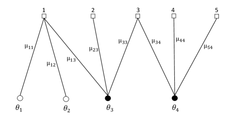
Figure 1: A network with 5 classes and 4 pools

Since ${\mathcal{I}}_{\mathsf{leaf}}$ is the set of leaf classes, then ${\mathcal{I}}_{\mathsf{leaf}}=\{2,4,5\}$ and $\widetilde{{\mathcal{J}}}=\{3,4\}$. These are the customer leaves to be removed in Step 1 of the algorithm and are shown as dashed edges.

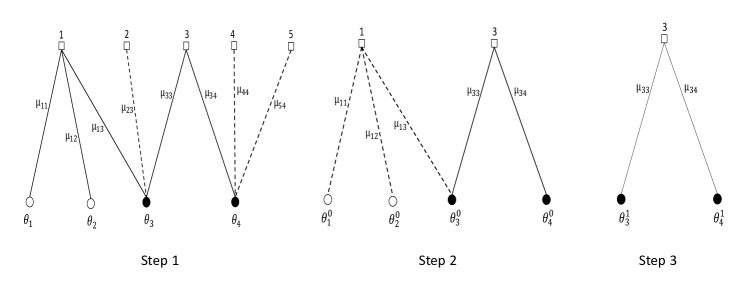
Figure 2: Illustration of the algorithm

In addition, the updates of the network parameters computed using Eq. 16 are given by

$$\begin{pmatrix}\theta_{1}^{0}\\[4.0pt] \theta_{2}^{0}\\[4.0pt] \theta_{3}^{0}\\[4.0pt] \theta_{4}^{0}\end{pmatrix}\,=\,\begin{pmatrix}\theta_{1}\\[4.0pt] \theta_{2}\\[4.0pt] \theta_{3}-\mu_{23}^{-1}(\vartheta_{p}p_{2}+\hat{\lambda}_{2})\\[4.0pt] \theta^{4}-\mu_{44}^{-1}(\vartheta_{p}p_{4}+\hat{\lambda}_{4})-\mu_{54}^{-1}(\vartheta_{p}p_{5}+\hat{\lambda}_{5})\end{pmatrix}\,.$$

In Step 2, class $1$ is selected i.e., $\imath_{1}=1$ and $\jmath_{1}=3$. The parameters are updated according to Eq. 18 and are given by

$$\begin{pmatrix}\theta_{3}^{1}\\[4.0pt] \theta_{4}^{1}\end{pmatrix}\,=\,\begin{pmatrix}\theta_{3}^{0}-\mu_{13}^{-1}\bigl{(}\hat{\lambda}_{1}+\vartheta_{p}p_{1}-\mu_{11}\theta_{1}^{0}-\mu_{12}\theta_{2}^{0}\bigr{)}\\[4.0pt] \theta_{4}^{0}\end{pmatrix}\,,$$

and class $1$ is removed together with the associated edges. The resulting network is shown in Step 3 and has only class $3$, i.e., $\hat{\imath}=3$. Therefore, the SWSS $\vartheta_{p}$ is computed using Eq. 21 as

$$\vartheta_{p}\,=\,-\hat{\lambda}_{3}+\mu_{33}\theta_{3}^{1}+\mu_{34}\theta_{4}^{1}\,.$$

Remark 3.4

In analogy to the definitions in the beginning of the section, we define the gain $\mathfrak{d}(j,j^{\prime})$ between any pair $j,j^{\prime}\in{\mathcal{J}}$, $j\neq j^{\prime}$, by

$$\mathfrak{d}(j,j^{\prime})\,\coloneqq\,\prod_{k=1}^{m-1}\frac{\mu_{i_{k+1}j_{k+1}}}{\mu_{i_{k+1}j_{k}}}\,,$$

where the product is evaluated over the analogous path $(j_{1},i_{2},j_{2},\dotsc,i_{m},j_{m})$ connecting $j\equiv j_{1}$ to $j^{\prime}\equiv j_{m}$ in ${\mathcal{G}}$. Suppose for simplicity that $\lambda_{i}^{n}=n\lambda_{i}$ and $\mu_{ij}^{n}=\mu_{ij}$. It follows from Eq. 14 that if we decrease $\hat{\nu}_{j}$ by an amount $\delta$ and increase $\hat{\nu}_{j^{\prime}}$ by an amount $\mathfrak{d}(j,j^{\prime})\delta$, then the value of $\vartheta_{p}$ stays the same. This has the following interpretation. The contribution of one server at pool $j$ in the stability of the network is the same as that of $\mathfrak{d}(j,j^{\prime})$ servers in pool $j^{\prime}$.

With $p$ a positive vector in $\varDelta_{I}$, we define

$$R_{i}\,\coloneqq\,\frac{\sum_{j\in{\mathcal{J}}}\mathfrak{d}(i,j)\theta_{j}-\sum_{\ell\in{\mathcal{I}}}\mathfrak{d}(i,\ell)\hat{\lambda}_{\ell}}{p_{i}}\,,\quad\text{and}\quad\varGamma_{i}\,\coloneqq\,\sum_{\ell\in{\mathcal{I}}}\mathfrak{d}(i,\ell)\frac{p_{\ell}}{p_{i}}$$

for $i\in{\mathcal{I}}$. Note that

$$\sum_{i\in{\mathcal{I}}}\varGamma_{i}^{-1}\,=\,\sum_{i\in{\mathcal{I}}}\frac{p_{i}}{\sum_{\ell\in{\mathcal{I}}}\mathfrak{d}(i,\ell)p_{\ell}}\,=\,\sum_{i\in{\mathcal{I}}}\frac{\mathfrak{d}(1,i)p_{i}}{\sum_{\ell\in{\mathcal{I}}}\mathfrak{d}(1,\ell)p_{\ell}}\,=\,1\,.$$ (25)

By Theorem 3.1 we have $\varGamma_{i}^{-1}\vartheta_{p}^{-1}=\frac{1}{R_{i}}$ for all $i\in{\mathcal{I}}$, and summing up this equality over $i\in{\mathcal{I}}$, and using Eq. 25, we obtain the following corollary.

Corollary 3.5

It holds that

$$\frac{1}{\vartheta_{p}}\,=\,\sum_{i\in{\mathcal{I}}}\frac{1}{R_{i}}\,.$$

As asserted in Corollary 3.5 the SWSS parameter $\vartheta_{p}$ is the harmonic mean of the variables $R_{i}$. This could be compared with the formula of the resistance of branches connected in parallel in electric circuits.

Remark 3.6

With $e_{i}\in\mathbb{R}^{I}$ as defined in Section 1.1, we have the identity $\vartheta_{e_{i}}=R_{i}$ for all $i\in{\mathcal{I}}$. In other words, $R_{i}$ is the maximum permissible safety staffing for class $i$ without allowing the safety staffing of the other classes to go negative.

4 Relating the SWSS to the Drift of the Diffusion Limit

In this section, we establish a characterization of the SWSS $\vartheta_{p}$ in terms of the parameters of the diffusion limit of the Markovian network. We also obtain an analogous characterization of $\vartheta_{p}^{n}$. The key results are in Propositions 4.2, 4.4, 4.7, and 4.9, and these are essential for the stability analysis in Sections 5 and 6.

For each $i\in{\mathcal{I}}$ and $j\in{\mathcal{J}}$, we let $X_{i}^{n}=\{X_{i}^{n}(t)\colon t\geq 0\}$ denote the total number of class $i$ customers in the system (both in service and in queue), $Z_{ij}^{n}=\{Z_{ij}^{n}(t),\,t\geq 0\}$ the number of class $i$ customers currently being served in pool $j$, $Q_{i}^{n}=\{Q_{i}^{n}(t),\,t\geq 0\}$ the number of class $i$ customers in the queue, and $Y_{j}^{n}=\{Y_{j}^{n}(t),\,t\geq 0\}$ the number of idle servers in server pool $j$. Let $X^{n}=(X_{i}^{n})_{i\in{\mathcal{I}}}$, $Y^{n}=(Y_{j}^{n})_{j\in{\mathcal{J}}}$, $Q^{n}=(Q_{i}^{n})_{i\in{\mathcal{I}}}$, and $Z^{n}=(Z_{ij}^{n})_{(i,j)\in{\mathcal{E}}}$. The process $Z^{n}$ is the scheduling control. Let $(x,z)\in\mathbb{Z}_{+}^{I}\times\mathbb{Z}^{{\mathcal{G}}}_{+}$ denote a state-action pair. We define

$$q_{i}(x,z)\,\coloneqq\,x_{i}-\sum_{j\in{\mathcal{J}}}z_{ij}\,,\quad i\in{\mathcal{I}}\,,\qquad y_{j}^{n}(z)\,\coloneqq\,N_{j}^{n}-\sum_{i\in{\mathcal{J}}}z_{ij}\,,\quad j\in{\mathcal{J}}\,,$$

and the (work-conserving) action space ${\mathcal{Z}^{n}}(x)$ by

$${\mathcal{Z}^{n}}(x)\,\coloneqq\,\bigl{\{}z\in\mathbb{Z}^{{\mathcal{G}}}_{+}\,\colon q_{i}(x,z)\wedge y_{j}^{n}(z)=0\,,~{}q_{i}(x,z)\geq 0\,,~{}y_{j}^{n}(z)\geq 0\quad\forall\,(i,j)\in{\mathcal{E}}\bigr{\}}\,.$$

4.1 The Diffusion Scaling

In this section, we first write the infinitesimal generator of the state process for the $n^{\mathrm{t}h}$ system in the form of Eq. 31 which is a linear expression involving second order and first order difference quotients. The coefficients of the first order difference quotients comprise the ‘drift’ of the infinitesimal generator. Then, in Proposition 4.2, we obtain an explicit form of the drift. The components of the constant term in the drift, which are denoted as $h^{n}_{i}$, are given in Eq. 30, and are equal to the diffusion-scaled difference between the service rates $\lambda_{i}^{n}$ and the service rate of class $i$ when the service allocations are chosen as the solution of Eq. LP. The constant term $h^{n}$ and the matrices $B_{1}^{n}$ and $B_{2}^{n}$ that describe the linear part of the drift, are used to characterize $\vartheta_{p}^{n}$ in Theorem 4.9 in Section 4.2.

We introduce some suitable notation to describe the diffusion scale. For additional details see Arapostathis and Pang (2019). With $\xi^{*}\in\mathbb{R}^{\mathcal{G}}_{+}$ being the solution of the Eq. LP, we define $\bar{z}^{n}\in\mathbb{R}^{{\mathcal{G}}}_{+}$ and $\bar{x}^{n}\in\mathbb{R}^{I}$ by

$$\bar{z}^{n}_{ij}\,\coloneqq\,\xi^{*}_{ij}N_{j}^{n}\,,\qquad\bar{x}^{n}_{i}\,\coloneqq\,\sum_{j\in{\mathcal{J}}}\bar{z}^{n}_{ij}\,,$$ (26)

and

$$\breve{x}^{n}\,=\,\breve{x}^{n}(x)\,\coloneqq\,\frac{x-\bar{x}^{n}}{\sqrt{n}}\,,\qquad\breve{z}^{n}\,=\,\breve{z}^{n}(z)\,\coloneqq\,\frac{z-\bar{z}^{n}}{\sqrt{n}}\,,$$ (27)

for $x\in\mathbb{Z}^{I}_{+}$ and $z\in{\mathcal{Z}^{n}}(x)$. We also let ${\mathscr{S}}^{n}$ denote the state space in the diffusion scale, that is, ${\mathscr{S}}^{n}\coloneqq\bigl{\{}\breve{x}\in{\mathbb{R}^{m}}\,\colon\sqrt{n}\breve{x}+\bar{x}^{n}\in\mathbb{Z}^{I}_{+}\bigr{\}}$. The diffusion-scaled variables are defined by

$$\breve{X}^{n}_{i}(t)\,\coloneqq\,\breve{x}^{n}\bigl{(}X_{i}^{n}(t)\bigr{)}\,,\quad\breve{Z}^{n}_{ij}(t)\,\coloneqq\,\breve{z}^{n}\bigl{(}Z_{ij}^{n}(t)\bigr{)}\,,\quad\breve{Q}^{n}_{i}(t)\,\coloneqq\,\frac{Q_{i}^{n}(t)}{\sqrt{n}}\,,\quad\text{and}\quad\breve{Y}^{n}_{j}(t)\,\coloneqq\,\frac{Y_{j}^{n}(t)}{\sqrt{n}}\,.$$ (28)

Under a stationary Markov policy $Z^{n}(t)=z(X^{n}(t))$ for some function $z\colon\mathbb{Z}^{I}_{+}\to\mathbb{Z}^{{\mathcal{G}}}_{+}$, the process $X^{n}$ is Markov with controlled generator

$$\mathscr{A}_{z}^{n}f(x)\,\coloneqq\,\sum_{i\in{\mathcal{I}}}\Biggl{(}\lambda_{i}^{n}\bigl{(}f(x+e_{i})-f(x)\bigr{)}+\sum_{j\in{\mathcal{J}}(i)}\mu_{ij}^{n}z_{ij}\bigl{(}f(x-e_{i})-f(x)\bigr{)}\Biggr{)}$$ (29)

for $f\in C(\mathbb{R}^{I})$ and $x\in\mathbb{Z}^{I}_{+}$.

We drop the explicit dependence on $n$ in the diffusion-scaled variables in order to simplify the notation. Note that a work-conserving stationary Markov policy $z$, that is a map $z\colon\mathbb{Z}^{I}_{+}\to\mathbb{Z}^{{\mathcal{G}}}_{+}$ such that $z(x)\in{\mathcal{Z}^{n}}(x)$ for all $x\in\mathbb{Z}_{+}^{I}$, gives rise to a stationary Markov policy $\breve{z}\colon{\mathscr{S}}^{n}\to\mathbb{R}^{\mathcal{G}}$, with

$$\breve{z}(\breve{x})\,\in\,{\breve{\mathcal{Z}}^{n}}(\breve{x})\,\coloneqq\,\bigl{\{}\breve{z}\,\colon\sqrt{n}\breve{z}+\bar{z}^{n}\in{\mathcal{Z}^{n}}(\sqrt{n}\breve{x}+\bar{x}^{n})\bigr{\}}\qquad\forall\,\breve{x}\in{\mathscr{S}}^{n}\,,$$

via Eq. 27 (and vice-versa). Let $h^{n}=(h^{n}_{1},\dotsc,h^{n}_{I})^{\mathsf{T}}$ be defined by

$$h^{n}_{i}\,\coloneqq\,\frac{1}{\sqrt{n}}\Biggl{(}\lambda^{n}_{i}-\sum_{j\in{\mathcal{J}}(i)}\mu_{ij}^{n}\xi^{*}_{ij}N_{j}^{n}\Biggr{)}\,.$$ (30)

By the assumptions on the parameters in Eqs. 1 and 2, we have $h^{n}_{i}\to h_{i}$ as $n\to\infty$, with $h_{i}$ as defined in Eq. 12. We let $h\coloneqq(h_{1},\dotsc,h_{I})^{\mathsf{T}}$. Using Eqs. 26, 27, 29, and 30 and rearranging terms, the controlled generator of the corresponding diffusion-scaled process can be written as

$$\breve{\mathscr{A}}_{\breve{z}}^{n}f(\breve{x})\,\coloneqq \,=\,\sum_{i\in{\mathcal{I}}}\frac{\lambda_{i}^{n}}{n}\,\frac{f\bigl{(}\breve{x}+\tfrac{1}{\sqrt{n}}e_{i}\bigr{)}-2f(\breve{x})+f\bigl{(}\breve{x}-\tfrac{1}{\sqrt{n}}e_{i}\bigr{)}}{n^{-1}}$$ (31)

$$\mspace{50.0mu}-\sum_{i\in{\mathcal{I}}}b^{n}_{i}(\breve{x},\breve{z})\,\frac{f\bigl{(}\breve{x}-\tfrac{1}{\sqrt{n}}e_{i}\bigr{)}-f(\breve{x})}{n^{-\nicefrac{{1}}{{2}}}}\,,\qquad\breve{x}\in{\mathscr{S}}^{n}\,,\ \breve{z}\in{\breve{\mathcal{Z}}^{n}}(\breve{x})\,,$$

where the ‘drift’ $b^{n}=(b_{1}^{n},\cdots,b_{I}^{n})^{\mathsf{T}}$ is given by

$$b^{n}_{i}(\breve{x},\breve{z})\,\coloneqq\,h_{i}^{n}-\sum_{j\in{\mathcal{J}}(i)}\mu_{ij}^{n}\breve{z}_{ij}\,,\quad\breve{z}\in{\breve{\mathcal{Z}}^{n}}(\breve{x})\,,\ i\in{\mathcal{I}}\,.$$ (32)

Definition 4.1

For $\breve{x}\in{\mathscr{S}}^{n}$ and $\breve{z}\in{\breve{\mathcal{Z}}^{n}}(\breve{x})$, we define

$$\breve{q}^{n}_{i}(\breve{x},\breve{z})\,\coloneqq\,\breve{x}_{i}-\sum_{j\in{\mathcal{J}}(i)}\breve{z}_{ij}\,,\quad i\in{\mathcal{I}}\,,\qquad\breve{y}^{n}_{j}(\breve{z})\,\coloneqq\,-\sum_{i\in{\mathcal{I}}(j)}\breve{z}_{ij}\,,\quad j\in{\mathcal{J}}\,,$$ (33)

and $\breve{\zeta}^{n}(\breve{x},\breve{z})\coloneqq\langle e,\breve{q}^{n}(\breve{x},\breve{z})\bigr{\rangle}\wedge\,\langle e,\breve{y}^{n}(\breve{z})\bigr{\rangle}$. We also let

$${\mathbb{U}}\,\coloneqq\,\varDelta_{I}\times\varDelta_{J}\,\coloneqq\,\bigl{\{}u^{c}\in\mathbb{R}^{I}_{+}\,\colon\,\langle e,u^{c}\rangle\,=\,1\bigr{\}}\times\bigl{\{}u^{s}\in\mathbb{R}^{J}_{+}\,\colon\,\langle e,u^{s}\rangle\,=\,1\bigr{\}}\,.$$ (34)

In the following proposition, we give an explicit expression of the drift $b^{n}$ and the some of its structural properties.

Proposition 4.2

For any $\breve{z}\in{\breve{\mathcal{Z}}^{n}}(\breve{x})$ with $\breve{x}\in{\mathscr{S}}^{n}$, there exists $u=u(\breve{x},\breve{z})\in{\mathbb{U}}$ such that the drift $b^{n}$ in Eq. 32 takes the form

$$b^{n}(\breve{x},\breve{z})\,=\,h^{n}-B_{1}^{n}\bigl{(}\breve{x}-\langle e,\breve{x}\rangle^{+}u^{c}\bigr{)}+B_{2}^{n}u^{s}\langle e,\breve{x}\rangle^{-}+\breve{\zeta}^{n}(\breve{x},\breve{z})\bigl{(}B_{1}^{n}u^{c}+B_{2}^{n}u^{s}\bigr{)}\,.$$ (35)

In Eq. 35, $h^{n}=(h^{n}_{1},\dotsc,h^{n}_{I})^{\mathsf{T}}$ with $h^{n}_{i}$ is as in Eq. 30, $B_{1}^{n}\in\mathbb{R}^{I\times I}$, and $B_{2}^{n}\in\mathbb{R}^{I\times J}$.

In addition, given any $(\hat{\imath},\hat{\jmath})\in{\mathcal{E}}$, there exists an ordered basis $\mathfrak{D}=\bigl{(}\alpha,(\beta)_{-\hat{\jmath}}\bigr{)}$, with $\alpha_{\hat{\imath}}$ being the last element of $\alpha$, with respect to which the matrices $B_{1}^{n}$ and $B_{2}^{n}$ take the following form:

• $B^{n}_{1}$ is a lower-diagonal $I\times I$ matrix with positive diagonal elements and $(B_{1})_{II}=\mu^{n}_{\hat{\imath}\hat{\jmath}}$;

• $B^{n}_{2}$ is an $I\times J$ matrix whose last column is identically zero.

Proof 4.3

Proof. Using Definition 4.1, it is easy to see that there exists $u=(u^{c},u^{s})\in{\mathbb{U}}$, depending on $\breve{x}\in{\mathscr{S}}^{n}$ and $\breve{z}\in{\breve{\mathcal{Z}}^{n}}(\breve{x})$, such that

$$\breve{q}^{n}(\breve{x},\breve{z})\,=\,\bigl{(}\breve{\zeta}^{n}(\breve{x},\breve{z})+\langle e,\breve{x}\rangle^{+}\bigr{)}\,u^{c}\,,\quad\text{and}\quad\breve{y}^{n}(\breve{z})\,=\,\bigl{(}\breve{\zeta}^{n}(\breve{x},\breve{z})+\langle e,\breve{x}\rangle^{-}\bigr{)}\,u^{s}\,.$$ (36)

Let ${\mathscr{D}}\coloneqq\bigl{\{}(\alpha,\beta)\in\mathbb{R}^{I}\times\mathbb{R}^{J}\,\colon\,\langle e,\alpha\rangle\,=\,\langle e,\beta\rangle\bigr{\}}$. Define the linear map $\Psi=[\Psi_{ij}]\colon{\mathscr{D}}\to\mathbb{R}^{I\times J}$ as the solution of

$$\sum_{j}\Psi_{ij}(\alpha,\beta)\,=\,\alpha_{i}\quad\forall i\in{\mathcal{I}}\,,\quad\text{and}\quad\sum_{i}\Psi_{ij}(\alpha,\beta)\,=\,\beta_{j}\quad\forall j\in{\mathcal{J}}\,,$$ (37)

with $\Psi_{ij}(\alpha,\beta)=0$ for $i\nsim j$. It is shown in Proposition A.2 of Atar (2005a) that if ${\mathcal{G}}$ is a tree, the linear map $\Psi$ is unique. Since $\bigl{(}\breve{x}-\breve{q}^{n}(\breve{x},\breve{z}),-\breve{y}^{n}(\breve{z})\bigr{)}\in{\mathscr{D}}$ by Eq. 33, using the linearity of the map $\Psi$ and Eqs. 36 and 37, it follows that

$$\breve{z} \,=\,\Psi\bigl{(}\breve{x}-\breve{q}^{n}(\breve{x},\breve{z}),-\breve{y}^{n}(\breve{z})\bigr{)}$$

$$\,=\,\Psi\bigl{(}\breve{x}-\langle e,\breve{x}\rangle^{+}u^{c},-\langle e,\breve{x}\rangle^{-}u^{s}\bigr{)}-\breve{\zeta}^{n}(\breve{x},\breve{z})\,\Psi(u^{c},u^{s})\,.$$

Consider the matrices $B_{1}^{n}\in\mathbb{R}^{I\times I}$ and $B_{2}^{n}\in\mathbb{R}^{I\times J}$ defined by

$$\sum_{j\in{\mathcal{J}}(i)}\mu^{n}_{ij}\Psi_{ij}(\alpha,\beta)\,=\,\bigl{(}B_{1}^{n}\alpha+B_{2}^{n}\beta\bigr{)}_{i}\,,\quad\forall\,i\in{\mathcal{I}}\,,\ \forall(\alpha,\beta)\in{\mathscr{D}}\,.$$ (38)

As shown in Arapostathis and Pang (2016, Lemma 4.3), given any $(\hat{\imath},\hat{\jmath})\in{\mathcal{E}}$, there exists an ordered basis $\mathfrak{D}=\bigl{(}\alpha,(\beta)_{-\hat{\jmath}}\bigr{)}$, $j\in{\mathcal{J}}$, where $(\beta)_{-\hat{\jmath}}=\{\beta_{\ell}\,,\,\ell\neq\hat{\jmath}\}$ and $\alpha_{\imath}$ is the last element of $\alpha$, such that the matrix $B^{n}_{1}$ in Eq. 38 satisfies assertion (a). It is also clear from the proof of the above lemma, that $B^{n}_{2}$ satisfies assertion (b). This completes the proof.

4.2 The Diffusion Limit

In this section we present some important properties of the drift of the limiting diffusion. This takes the form of the piecewise-affine function given in Eq. 43. The coefficients $h$, $B_{1}$, and $B_{2}$ are the limits of $h^{n}$, $B_{1}^{n}$, and $B_{2}^{n}$ in Eq. 35, respectively, as $n\to\infty$. Two additional important results are presented in this section: Theorem 4.7 which characterizes the gains $\mathfrak{d}(i,\ell)$ for $i,\ell\in{\mathcal{I}}$ in terms of the matrix $B_{1}$, and Theorem 4.9 which obtains an analogous characterization of the SWSS parameters $\vartheta_{p}$ and $\vartheta^{n}_{p}$.

To discuss the diffusion limit we need the concept of joint work conservation. We say that an action $\breve{z}\in{\breve{\mathcal{Z}}^{n}}(\breve{x})$ is jointly work conserving (JWC), if $\breve{\zeta}^{n}(\breve{x},\breve{z})=0$ , i.e., a scheduling rule for which either there are no customers in the queues, or no server in the system is idle. Simple examples show that it is not possible to specify such an action on the whole state space. However, as shown in Atar (2005b, Lemma 3), there exists $M_{0}>0$ such that the collection of sets $\breve{{\mathscr{X}}}^{n}$ defined by

$$\breve{{\mathscr{X}}}^{n}\,\coloneqq\,\bigl{\{}\breve{x}\in{\mathscr{S}}^{n}\,\colon\lVert\breve{x}\rVert_{1}\leq M_{0}\,\sqrt{n}\bigr{\}}$$ (39)

has the following property: For any $\breve{x}\in\breve{{\mathscr{X}}}^{n}$ and a pair $(\breve{q},\breve{y})$ such that $\sqrt{n}\breve{q}\in\mathbb{Z}^{I}_{+}$, $\sqrt{n}\breve{y}\in\mathbb{Z}^{J}_{+}$, and

$$\langle e,\breve{q}\rangle\wedge\langle e,\breve{y}\rangle\,=\,0\,,\quad\langle e,\breve{x}-\breve{q}\rangle\,=\,\langle e,-\breve{y}\rangle\,,\quad\text{and}\quad\breve{y}_{j}\sqrt{n}\,\leq\,N^{n}_{j}\,,\quad j\in{\mathcal{J}}\,,$$

it holds that $\Psi(\breve{x}-\breve{q},-\breve{y})\in{\breve{\mathcal{Z}}^{n}}(\breve{x})$.

Under any stationary Markov scheduling policy that is jointly work-conserving in the set $\breve{{\mathscr{X}}}^{n}$, the diffusion-scaled state process $\breve{X}^{n}$ converges weakly to a limit $X$ described as follows. For $u\in{\mathbb{U}}$, let $\breve{\Psi}[u]\colon\mathbb{R}^{I}\to\mathbb{R}^{{\mathcal{G}}}$ be defined by

$$\breve{\Psi}[u](x)\,\coloneqq\,\Psi(x-\langle e,x\rangle^{+}u^{c},-\langle e,x\rangle^{-}u^{s})\,,$$ (40)

where $\Psi$ is as in Eq. 37. The limiting controlled diffusion $X$ is given by the Itô equation

$$dX_{t}\,=\,b(X_{t},U_{t})\,\mathrm{d}{t}+\Sigma\,\mathrm{d}W_{t}\,,$$ (41)

where $W$ is an $I$-dimensional standard Wiener process, and $\Sigma\coloneqq\operatorname*{diag}\bigl{(}\sqrt{2\lambda_{1}},\dotsc,\sqrt{2\lambda_{I}}\bigr{)}$. The drift $b\colon\mathbb{R}^{I}\times{\mathbb{U}}\to\mathbb{R}^{I}$ takes the form

$$b_{i}(x,u)\,=\,b_{i}\bigl{(}x,(u^{c},u^{s})\bigr{)}\,\coloneqq\,h_{i}-\sum_{j\in{\mathcal{J}}(i)}\mu_{ij}\breve{\Psi}_{ij}[u](x)\qquad\forall\,i\in{\mathcal{I}}\,,$$ (42)

where $\breve{\Psi}_{ij}[u]$ is as in Eq. 40 and $h_{i}$ is given by Eq. 12. This result was first shown in Atar (2005a, b). We focus on the class $\mathfrak{U}_{\mathrm{sm}}$ of stationary Markov controls, that is, $U_{t}=v(X_{t})$ for some measurable function $v\colon\mathbb{R}^{I}\to{\mathbb{U}}$.

The following proposition is the exact analog of Proposition 4.2, and follows by taking limits as $n\to\infty$ in Eq. 35 and employing the convergence of the parameters in Eqs. 1 and 2.

Proposition 4.4

Given any $(\hat{\imath},\hat{\jmath})\in{\mathcal{E}}$, there exists an ordered basis $\mathfrak{D}=\bigl{(}\alpha,(\beta)_{-\hat{\jmath}}\bigr{)}$, with $\alpha_{\hat{\imath}}$ being the last element of $\alpha$, with respect to which the drift $b$ in Eq. 42 has the representation

$$b(x,u)\,=\,h-B_{1}(x-\langle e,x\rangle^{+}u^{c})+\langle e,x\rangle^{-}B_{2}u^{s}\,,$$ (43)

where

• $h=(h_{1},\dotsc,h_{I})^{\mathsf{T}}$ and $h_{i}$ is as in Eq. 12,

• $B_{1}$ is a lower-diagonal $I\times I$ matrix with positive diagonal elements and $(B_{1})_{II}=\mu_{\hat{\imath}\hat{\jmath}}$ ,

• $B_{2}$ is an $I\times J$ matrix whose last column is identically zero.

For $f\in C^{2}(\mathbb{R}^{m})$, we define

$$\mathscr{A}_{u}f(x)\,\coloneqq\,\frac{1}{2}\operatorname*{trace}\bigl{(}\Sigma\Sigma^{\mathsf{T}}\nabla^{2}f(x)\bigr{)}+\bigl{\langle}b(x,u),\nabla f(x)\bigr{\rangle}\,,$$ (44)

with $\nabla^{2}f$ denoting the Hessian of $f$.

Remark 4.5

We remark that Eq. 28 differs from the usual definition of the diffusion-scaled processes found in the literature (see Atar (2005b) and Arapostathis and Pang (2016, 2018, 2019)). We refer to the processes $\breve{X}^{n}_{i}$ as the “re-centered” diffusion-scaled processes. One may also center the process $X^{n}_{i}$ around $nx^{*}_{i}$ where $x^{*}$ is defined in Eq. 4. It is clear that the limit processes using these different centering terms only differ in the drift by a constant, and therefore they are equivalent as far as their ergodic properties are concerned. See also Remark 6.6.

Remark 4.6

Note that if the networks have renewal arrivals and the service times are exponential, we again obtain a diffusion limit for the above diffusion-scaled processes, which has the same drift as the Markovian case, and whose covariance matrix captures the variability in the arrivals processes. In particular, if the class-$i$ arrival process $A^{n}_{i}$ is renewal with interarrival times of rate $\lambda^{n}_{i}$ (satisfying Eqs. 1 and 2) and variance $(\sigma^{n}_{i})^{2}$ (satisfying $\sigma^{n}_{i}\to\sigma_{i}>0$ as $n\to\infty$), then

$$\hat{A}^{n}_{i}(t)\,=\,n^{\nicefrac{{1}}{{2}}}(A^{n}_{i}(t)-\lambda^{n}_{i}t)\,\Rightarrow\,\hat{A}_{i}(t)\,=\,W_{i}(\lambda_{i}c^{2}_{a,i}t)\,,$$

where $W_{i}$ is a standard Brownian motion, and $c^{2}_{a,i}\coloneqq\lambda_{i}^{2}\sigma_{i}^{2}$. As a consequence, the covariance matrix $\Sigma$ in Eq. 41 takes the form $\Sigma=\operatorname*{diag}\bigl{(}\bigl{(}\lambda_{1}(1+c_{a,1}^{2})\bigr{)}^{\nicefrac{{1}}{{2}}},\dotsc,\bigl{(}\lambda_{I}(1+c_{a,I}^{2})\bigr{)}^{\nicefrac{{1}}{{2}}}\bigr{)}\,.$ Thus, the results in Theorem 4.7 also hold for the networks with renewal arrivals and exponential service times. The same applies to the results regarding the limiting controlled diffusion in Theorems 5.3 and 6.3. See also Remark 6.13 for the results concerning the diffusion-scaled processes.

The following result is essential in proving the main theorem of this section. Recall the definition in Eq. 13.

Theorem 4.7

It holds that

$$\mathfrak{d}(i,\ell)\,=\,\frac{\bigl{(}e^{\mathsf{T}}B_{1}^{-1}\bigr{)}_{\ell}}{\bigl{(}e^{\mathsf{T}}B_{1}^{-1}\bigr{)}_{i}}\qquad\forall\,i,\ell\in{\mathcal{I}}\,.$$ (45)

In addition, $\bigl{(}e^{\mathsf{T}}B_{1}^{-1}\bigr{)}_{i}>0$ for all $i\in{\mathcal{I}}$.

Proof 4.8

Proof. We start with the following observation: Let $\vartheta_{p}$, $\kappa=[\kappa_{ij}]\in\mathbb{R}^{{\mathcal{G}}}$ be the unique solution of Eq. LP^′. This means that $\sum_{j\in{\mathcal{J}}(i)}\mu_{ij}\kappa_{ij}=\hat{\lambda}_{i}+\vartheta_{p}p_{i}$ and $\sum_{i\in{\mathcal{I}}(j)}\kappa_{ij}=\theta_{j}$ for $i\in{\mathcal{I}}$ and $j\in{\mathcal{J}}$. Let $\alpha_{i}=\sum_{j}\kappa_{ij}$ and note that $e^{\mathsf{T}}\alpha=e^{\mathsf{T}}\theta$ where $\alpha=(\alpha_{i})_{i\in{\mathcal{I}}}$ and $\theta=(\theta_{j})_{j\in{\mathcal{J}}}$.

Using a similar approach to Eqs. 37 and 38, it follows that $\kappa_{ij}=\Psi_{ij}(\alpha,\theta)$ and $B_{1}\alpha+B_{2}\theta=\sum_{j\in{\mathcal{J}}(i)}\mu_{ij}\Psi_{ij}(\alpha,\theta)=\hat{\lambda}+\vartheta_{p}p$. Inverting $B_{1}$ and using that $e^{T}\alpha=e^{T}\theta$, one reaches that

$$\vartheta_{p}e^{T}B_{1}^{-1}p=e^{T}\theta+e^{T}B_{1}^{-1}(-\hat{\lambda}+B_{2}\theta).$$ (46)

This means that $\vartheta_{p}e^{T}B_{1}^{-1}p$ remains constant when $p$ varies. Using Eqs. 14 and 46 we get that $e^{T}B_{1}^{-1}p=c\sum_{\ell\in{\mathcal{I}}}\mathfrak{d}(i,\ell)p_{\ell}$ for every positive probability vector $p$ where $c$ is a constant independent of $p$. This of course implies that $\bigl{(}e^{T}B_{1}^{-1}\bigr{)}_{\ell}=c\,\mathfrak{d}(i,\ell)$ for $\ell\in{\mathcal{I}}$. It remains to note that $\mathfrak{d}(i,i)=1$ by definition, see Eq. 13, to conclude that $c=\bigl{(}e^{T}B_{1}^{-1}\bigr{)}_{i}$.

To prove the last assertion of the theorem, note that $\bigl{(}e^{\mathsf{T}}B_{1}^{-1}\bigr{)}_{I}>0$ since $B_{1}$ is a lower diagonal matrix with positive elements. Thus, using Eq. 45, we obtain $\bigl{(}e^{\mathsf{T}}B_{1}^{-1}\bigr{)}_{i}=\mathfrak{d}(I,i)\bigl{(}e^{\mathsf{T}}B_{1}^{-1}\bigr{)}_{I}>0$ and this concludes the proof.

Theorem 4.9

The variables $\vartheta_{p}$ and $\vartheta^{n}_{p}$ in Definition 2.1 satisfy

$$\vartheta_{p}\,=\,-\frac{\langle e,B_{1}^{-1}h\rangle}{\langle e,B_{1}^{-1}p\rangle}\quad\text{and\ \ }\vartheta^{n}_{p}\,=\,-\frac{\langle e,(B_{1}^{n})^{-1}h^{n}\rangle}{\langle e,(B_{1}^{n})^{-1}p\rangle}\,,$$ (47)

where $h=(h_{i})_{i\in{\mathcal{I}}}$ is given by Eq. 12, $h^{n}$ is defined in Eq. 30, and $p\in\varDelta_{I}$ is a positive vector.

Proof 4.10

Proof. By Theorem 4.7, we have

$$e^{\mathsf{T}}B_{1}^{-1}p\,=\,\sum_{\ell\in{\mathcal{I}}}\bigl{(}e^{\mathsf{T}}B_{1}^{-1}\bigr{)}_{\ell}\,p_{\ell}\,=\,\bigl{(}e^{\mathsf{T}}B_{1}^{-1}\bigr{)}_{i}\sum_{\ell\in{\mathcal{I}}}\mathfrak{d}(i,\ell)p_{\ell}\,,$$

and $e^{\mathsf{T}}B_{1}^{-1}h=\bigl{(}e^{\mathsf{T}}B_{1}^{-1}\bigr{)}_{i}\sum_{\ell\in{\mathcal{I}}}\mathfrak{d}(i,\ell)h_{\ell}$. Combining these we obtain

$$-\frac{e^{\mathsf{T}}B_{1}^{-1}h}{e^{\mathsf{T}}B_{1}^{-1}p} \,=\,\frac{\sum_{\ell\in{\mathcal{I}}}\mathfrak{d}(i,\ell)\sum_{j\in{\mathcal{J}}(\ell)}\Bigl{(}\mu_{\ell j}\xi^{*}_{\ell j}\hat{\nu}_{\ell j}+\hat{\mu}_{\ell j}z^{*}_{\ell j}\Bigr{)}-\sum_{\ell\in{\mathcal{I}}}\mathfrak{d}(i,\ell)\hat{\lambda}_{\ell}}{\sum_{\ell\in{\mathcal{I}}}\mathfrak{d}(i,\ell)p_{\ell}}\,=\,\vartheta_{p}\,,$$

where in the last equality we used $\sum_{i\in{\mathcal{I}}(j)}\xi^{*}_{ij}=1$. The same approach is used for $\vartheta^{n}_{p}$, thus establishing Eq. 47.

4.3 Some Examples

In this part, we present some applications of Theorems 3.1 and 4.9 by computing explicitly the SWSS parameter for some networks. We also give simple interpretations in the special case when $\lambda_{i}^{n}=n\lambda_{i}$ and $\mu^{n}_{ij}=\mu_{ij}$, or equivalently, if $\hat{\lambda}_{i}=0$, $\hat{\mu}_{ij}=0$, and $\theta_{j}=\hat{\nu}_{j}$ for all $i\in{\mathcal{I}}$ and $j\in{\mathcal{J}}$.

Example 4.11 (The ‘N’ Network)

For this network the SWSS parameter is given by

$$\vartheta_{p}\,=\,\frac{\mu_{22}}{\mu_{12}\,p_{2}+\mu_{22}\,p_{1}}\biggl{(}\mu_{11}\theta_{1}+\mu_{12}\theta_{2}-\hat{\lambda}_{1}-\frac{\mu_{12}}{\mu_{22}}\hat{\lambda}_{2}\biggr{)}\,,$$

with

$$\kappa_{11}^{*}\,=\,\theta_{1}\,,\quad\kappa_{22}^{*}\,=\,\frac{\hat{\lambda}_{2}+\vartheta_{p}\,p_{2}}{\mu_{22}}\,,\quad\kappa_{12}^{*}\,=\,\theta_{2}-\kappa_{22}^{*}\,.$$

In this case, the $B_{1}$ matrix is given by $B_{1}=\operatorname*{diag}(\mu_{12},\mu_{22})$ and the vector $h$ is given by

$$h\,=\,\begin{pmatrix}\hat{\lambda}_{1}-\mu_{11}\xi^{*}_{11}\hat{\nu}_{1}-\hat{\mu}_{11}z^{*}_{11}-\mu_{12}\xi^{*}_{12}\hat{\nu}_{2}-\hat{\mu}_{12}z^{*}_{12}\\[3.0pt] \hat{\lambda}_{2}-\mu_{22}\xi^{*}_{22}\hat{\nu}_{2}-\hat{\mu}_{22}z^{*}_{22}\end{pmatrix}\,,$$

where $\xi^{*}_{11}=1$, $\xi^{*}_{12}+\xi^{*}_{22}=1$. A simple calculation confirms that $\vartheta_{p}=-\frac{\langle e,B_{1}^{-1}h\rangle}{\langle e,B_{1}^{-1}p\rangle}$. In the special case mentioned above, one can see that a necessary and sufficient condition for $\vartheta_{p}>0$ is $\mu_{11}\hat{\nu}_{1}+\mu_{12}\hat{\nu}_{2}>0$. If $\hat{\nu}_{1}<0$ and $\hat{\nu}_{2}>0$, by rewriting the condition as $\frac{\mu_{11}\hat{\nu}_{1}}{\mu_{12}}+\hat{\nu}_{2}>0$, we see that, the first term represents the service capacity required for class $1$ at pool $2$ to be reallocated, and thus, the sum being positive means that there is an allowance at pool $2$ for class $1$ to be served. Similarly for the case when $\hat{\nu}_{1}>0$ and $\hat{\nu}_{2}<0$.

Example 4.12 (The ‘M’ Network)

We obtain the SWSS parameter

$$\vartheta_{p}\,=\,\frac{\mu_{22}}{\mu_{22}p_{1}+\mu_{12}p_{2}}\Bigl{(}\mu_{11}\theta_{1}+\mu_{12}\theta_{2}+\frac{\mu_{12}\mu_{23}}{\mu_{22}}\theta_{3}-\hat{\lambda}_{1}-\frac{\mu_{12}}{\mu_{22}}\hat{\lambda}_{2}\Bigr{)}\,,$$

with

$$\kappa_{11}^{*}\,=\,\theta_{1}\,,\quad\kappa_{23}^{*}\,=\,\theta_{3}\,,\quad\kappa_{12}^{*}\,=\,\theta_{2}-\kappa_{22}^{*}\,,\quad\kappa_{22}^{*}\,=\,\frac{\hat{\lambda}_{2}+\vartheta_{p}\,p_{2}-\mu_{23}\theta_{3}}{\mu_{22}}\,.$$

In this case, the $B_{1}$ matrix is given by $B_{1}=\operatorname*{diag}(\mu_{12},\mu_{22})$, and the vector $h$ is given by

$$h\,=\,\begin{pmatrix}\hat{\lambda}_{1}-\mu_{11}\xi^{*}_{11}\hat{\nu}_{1}-\hat{\mu}_{11}z^{*}_{11}-\mu_{12}\xi^{*}_{12}\hat{\nu}_{2}-\hat{\mu}_{12}z^{*}_{12}\\[3.0pt] \hat{\lambda}_{2}-\mu_{22}\xi^{*}_{22}\hat{\nu}_{2}-\hat{\mu}_{22}z^{*}_{22}-\mu_{23}\xi^{*}_{23}\hat{\nu}_{3}-\hat{\mu}_{23}z^{*}_{23}\end{pmatrix}\,,$$

where $\xi^{*}_{11}=1$, $\xi^{*}_{12}+\xi^{*}_{22}=1$, $\xi^{*}_{23}=1$. It is clear that $\vartheta_{p}=-\frac{\langle e,B_{1}^{-1}h\rangle}{\langle e,B_{1}^{-1}p\rangle}$. In the special case, a necessary and sufficient condition for $\vartheta_{p}>0$ is

$$\mu_{11}\hat{\nu}_{1}+\mu_{12}\hat{\nu}_{2}+\frac{\mu_{12}\mu_{23}}{\mu_{22}}\hat{\nu}_{3}\,>\,0\iff\frac{\mu_{11}}{\mu_{12}}\hat{\nu}_{1}+\hat{\nu}_{2}+\frac{\mu_{23}}{\mu_{22}}\hat{\nu}_{3}\,>\,0\,.$$

This condition also has a very intuitive interpretation. For instance, if $\hat{\nu}_{1}<0\,,\hat{\nu}_{3}<0$ and $\hat{\nu}_{2}>0$, then the first and third terms represent the service capacity required for class 1 and class 3 at server pool 2, respectively, and the sum being positive means that the safety staffing at pool 2 is sufficient to serve these additional service requirements.

Example 4.13 (The ‘W’ Network)

The SWSS parameter is given by

$$\vartheta_{p}\,=\,\frac{1}{\frac{\mu_{21}}{\mu_{11}}p_{1}+p_{2}+\frac{\mu_{22}}{\mu_{32}}p_{3}}\Bigl{(}\mu_{21}\theta_{1}+\mu_{22}\theta_{2}-\frac{\mu_{21}}{\mu_{11}}\hat{\lambda}_{1}-\hat{\lambda}_{2}-\frac{\mu_{22}}{\mu_{32}}\hat{\lambda}_{3}\Bigr{)}\,,$$

with

$$\kappa_{11}^{*}\,=\,\frac{\hat{\lambda}_{1}+\vartheta_{p}\,p_{1}}{\mu_{11}}\,,\quad\kappa_{21}^{*}\,=\,\theta_{1}-\kappa_{11}^{*}\,,\quad\kappa_{32}^{*}\,=\,\frac{\hat{\lambda}_{3}+\vartheta_{p}\,p_{3}}{\mu_{32}}\,\quad\kappa_{22}^{*}\,=\,\theta_{2}-\kappa_{32}^{*}.$$

In this case, the $B_{1}$ matrix and $h$ vector are given by

$$B_{1}\,=\,\begin{pmatrix}\mu_{11}&0&0\\[3.0pt] \mu_{22}-\mu_{21}&\mu_{22}&0\\[3.0pt] 0&0&\mu_{32}\end{pmatrix}\qquad\text{and}\qquad h\,=\ \begin{pmatrix}\hat{\lambda}_{1}-\mu_{11}\xi^{*}_{11}\hat{\nu}_{1}-\hat{\mu}_{11}z^{*}_{11}\\[3.0pt] \hat{\lambda}_{2}-\mu_{21}\xi^{*}_{21}\hat{\nu}_{1}-\mu_{22}\xi^{*}_{22}\hat{\nu}_{2}-\hat{\mu}_{21}z^{*}_{21}-\hat{\mu}_{22}z^{*}_{22}\\[3.0pt] \hat{\lambda}_{3}-\mu_{32}\xi^{*}_{32}\hat{\nu}_{3}-\hat{\mu}_{32}z^{*}_{32}\end{pmatrix}\,,$$

where $\xi^{*}_{11}+\xi^{*}_{21}=1$ and $\xi^{*}_{22}+\xi^{*}_{32}=1$. A simple calculation confirms that $\vartheta_{p}=-\frac{\langle e,B_{1}^{-1}h\rangle}{\langle e,B_{1}^{-1}p\rangle}$. In the special case, a necessary and sufficient condition for $\vartheta_{p}>0$ is $\mu_{21}\hat{\nu}_{1}+\mu_{22}\hat{\nu}_{2}>0$.

5 Transience

In this part, we show that both the diffusion limit and diffusion-scaled state process of the $n^{\mathrm{t}h}$ system are transient when $\vartheta_{p}<0$ and $\vartheta^{n}_{p}<0$, respectively. In addition, we show that they cannot be positive recurrent when $\vartheta_{p}=0$ and $\vartheta^{n}_{p}=0$, respectively. We start with the following important lemma.

Lemma 5.1

The drift in Eq. 43 satisfies $\inf_{u^{s}\in\varDelta_{s}}\,\bigl{(}1+\bigl{\langle}e,B_{1}^{-1}B_{2}u^{s}\bigr{\rangle}\bigr{)}>0$, where $\varDelta_{J}$ is as in Eq. 34.

Proof 5.2

Proof. This proof is motivated by that of Theorem 4.7. Let $\tilde{\vartheta}_{p}\in\mathbb{R}_{+}$, $\tilde{\kappa}=[\tilde{\kappa}_{ij}]\in\mathbb{R}_{+}^{{\mathcal{G}}}$ be the unique solution of the following optimization problem

maximize $$\quad\tilde{\vartheta}_{p} {}^{{}^{\prime\prime}}$$ (LP)

subject to $$\quad 0\,\leq\,\sum_{j\in{\mathcal{J}}(i)}\mu_{ij}\tilde{\kappa}_{ij}-\tilde{\vartheta}_{p}\,p_{i}\qquad\forall\,i\in{\mathcal{I}}\,,$$

$$\sum_{i\in{\mathcal{I}}(j)}\tilde{\kappa}_{ij}\,=\,u^{s}_{j}\,,\qquad\forall j\in{\mathcal{J}},u^{s}\in\varDelta_{s}\,.$$

Note that if we set $\hat{\lambda}_{i}=0$, $\theta_{j}=u^{s}_{j}$ in the proof of Theorem 4.7, the same conclusion holds as in Eq. 46, i.e.,

$$\tilde{\vartheta}_{p}e^{T}B_{1}^{-1}p=e^{T}u^{s}+e^{T}B_{1}^{-1}B_{2}u^{s}=1+e^{T}B_{1}^{-1}B_{2}u^{s},$$

where the last equality holds because $u^{s}\in\varDelta_{s}$. The proof is concluded by noting that $\tilde{\vartheta}_{p}\in\mathbb{R}_{+}$ and that we have shown in Theorem 4.7 that $\bigl{(}e^{\mathsf{T}}B_{1}^{-1}\bigr{)}_{i}>0$ for all $i\in{\mathcal{I}}$.

We first show that $\vartheta_{p}<0$ implies transience for the diffusion limit.

Theorem 5.3

Suppose that $\vartheta_{p}<0$. Then the limiting diffusion ${\{X_{t}\}_{t\geq 0}}$ in Eq. 41 is transient under any stationary Markov control. In addition, if $\vartheta_{p}=0$, then $\{X(t)\}_{t\geq 0}$ cannot be positive recurrent.

Proof 5.4

Proof. In the following, note that the function $H(x)$ is a test function and it is chosen such that $\mathscr{A}_{u}H(x)>0$. Let $H(x)\coloneqq\tanh\bigl{(}\beta\langle e,B_{1}^{-1}x\rangle\bigr{)}$, with $\beta>0$. Then

$$\operatorname*{trace}\bigl{(}\Sigma\Sigma^{\mathsf{T}}\nabla^{2}H(x))\bigr{)}\,=\,\beta^{2}\tanh^{\prime\prime}\bigl{(}\beta\langle e,B_{1}^{-1}x\rangle\bigr{)}\bigl{\lvert}\Sigma^{\mathsf{T}}B_{1}^{-1}e\bigr{\rvert}^{2}\,,$$

where we recall $\Sigma\coloneqq\operatorname*{diag}\bigl{(}\sqrt{2\lambda_{1}},\dotsc,\sqrt{2\lambda_{I}}\bigr{)}$. We have

$$\mathscr{A}_{u}H(x) \,=\,\frac{1}{2}\operatorname*{trace}\bigl{(}\Sigma\Sigma^{\mathsf{T}}\nabla^{2}H(x)\bigr{)}+\bigl{\langle}b(x,u),\nabla H(x)\bigr{\rangle}$$ (48)

$$\,=\,-\beta^{2}\frac{\tanh\bigl{(}\beta\langle e,B_{1}^{-1}x\rangle\bigr{)}}{\cosh^{2}\bigl{(}\beta\langle e,B_{1}^{-1}x\rangle\bigr{)}}\lvert\Sigma^{\mathsf{T}}B_{1}^{-1}e\rvert^{2}$$

$$\mspace{80.0mu}+\frac{\beta}{\cosh^{2}\bigl{(}\beta\langle e,B_{1}^{-1}x\rangle\bigr{)}}\biggl{(}\bigl{\langle}e,B_{1}^{-1}h\bigr{\rangle}+\langle e,x\rangle^{-}\Bigl{(}1+\bigl{\langle}e,B_{1}^{-1}B_{2}u^{s}\bigr{\rangle}\Bigr{)}\biggr{)}\,.$$

Thus, for $0<\beta<\langle e,B_{1}^{-1}h\rangle\,\lvert\Sigma^{\mathsf{T}}B_{1}^{-1}e\rvert^{-2}$, we obtain $\mathscr{A}_{u}H(x)>0$ by Lemma 5.1 and using Theorems 4.7 and 4.9 to conclude that $\langle e,B_{1}^{-1}h\rangle>0$. Therefore, $\{H\bigl{(}X_{t}\bigr{)}\}_{t\geq 0}$ is a bounded submartingale, so it converges almost surely. Since $X$ is irreducible, it can be either recurrent or transient. If it is recurrent, then $H$ should be constant a.e. in $\mathbb{R}^{I}$, which is not the case. Thus $X$ is transient.

We now turn to the case where $\vartheta_{p}=0$. Suppose that the process $\{X(t)\}_{t\geq 0}$ (under some stationary Markov control) has an invariant probability measure $\uppi(\mathrm{d}{x})$. It is well known that $\uppi$ must have a positive density. Let $g_{1}(x)$ and $g_{2}(x)$ denote respectively the first and the second terms on the right hand side of Eq. 48. Applying Itô’s formula to Eq. 48, we obtain

$$\operatorname{\mathbb{E}}^{\uppi}\bigl{[}H(X_{t\wedge\tau_{r}})\bigr{]}-H(x)\,=\,\sum_{i=1,2}\operatorname{\mathbb{E}}^{\uppi}\Biggl{[}\int_{0}^{t\wedge\tau_{r}}g_{i}(X_{s})\mathrm{d}s\Biggr{]}\,,$$ (49)

where $\tau_{r}$ denotes the first exit time from the ball $B_{r}$ of radius $r$ centered at $0$. Note that $g_{1}(x)$ is bounded and $g_{2}(x)$ is non-negative. Thus using dominated and monotone convergence, we can take limits in Eq. 49 as $r\to\infty$ for the terms on the right side to obtain

$$\int_{{\mathbb{R}^{m}}}H(x)\uppi(\mathrm{d}{x})-H(x)\,=\,t\sum_{i=1,2}\int_{{\mathbb{R}^{m}}}g_{i}(x)\uppi(\mathrm{d}{x}),\qquad t\geq 0\,.$$

Since $H(x)$ is bounded, we can divide both sides by $t$ and $\beta$ and take the limit as $t\to\infty$ to get

$$\int_{{\mathbb{R}^{m}}}\beta^{-1}g_{1}(x)\uppi(\mathrm{d}{x})+\int_{{\mathbb{R}^{m}}}\beta^{-1}g_{2}(x)\uppi(\mathrm{d}{x})\,=\,0\,.$$ (50)

Since $\beta^{-1}g_{1}(x)$ tends to 0 uniformly in $x$ as $\beta\searrow 0$, the first term on the left hand side of Eq. 50 vanishes as $\beta\searrow 0$. However, since $\beta^{-1}g_{2}(x)$ is bounded away from $0$ on the open set $\{x\in{\mathbb{R}^{m}}\colon\langle e,x\rangle^{-}>1\}$, this contradicts the fact that $\uppi(\mathrm{d}{x})$ has full support.

The proof of the following corollary is analogous to that of Lemma 5.1.

Corollary 5.5

The drift in Eq. 35 satisfies $\inf_{u^{s}\in\varDelta_{s}}\,\bigl{(}1+\bigl{\langle}e,(B_{1}^{n})^{-1}B_{2}^{n}u^{s}\bigr{\rangle}\bigr{)}>0$.

Theorem 5.6

Suppose that $\vartheta_{p}^{n}<0$. Then the diffusion-scaled state process $\{\breve{X}^{n}(t)\}_{t\geq 0}$ of the $n^{\mathrm{th}}$ system is transient under any stationary Markov scheduling policy. In addition, if $\vartheta_{p}^{n}=0,$ the process $\{\breve{X}^{n}(t)\}_{t\geq 0}$ cannot be positive recurrent.

Proof 5.7

Proof. The proof mimics that of Theorem 5.3. We apply the function $H(x)=\tanh\bigl{(}\beta\langle e,(B_{1}^{n})^{-1}x\rangle\bigr{)}$ to the operator $\breve{\mathscr{A}}^{n}_{z}$ in Eq. 31, and use the identity

$$H\Bigl{(}x\pm\tfrac{1}{\sqrt{n}}e_{i}\Bigr{)}-H(x)\mp\frac{1}{\sqrt{n}}\partial_{x_{i}}H(x)\,=\,\frac{1}{n}\int_{0}^{1}(1-t)\,\partial_{x_{i}x_{i}}H\Bigl{(}x\pm\tfrac{t}{\sqrt{n}}e_{i}\Bigr{)}\,\mathrm{d}{t}$$

to express the first and second order incremental quotients, together with Eq. 35 which implies that

$$\bigl{\langle}b^{n}(\breve{x},\breve{z}),\nabla H(\breve{x})\bigr{\rangle}\,=\,\frac{\beta}{\cosh^{2}\bigl{(}\beta\langle e,(B_{1}^{n})^{-1}\breve{x}\rangle\bigr{)}}\biggl{(}\bigl{\langle}e,(B_{1}^{n})^{-1}h^{n}\bigr{\rangle}\\ +\bigl{(}\breve{\zeta}^{n}(\breve{x},\breve{z})+\langle e,\breve{x}\rangle^{-}\bigr{)}\Bigl{(}1+\bigl{\langle}e,(B_{1}^{n})^{-1}B_{2}^{n}u^{s}\bigr{\rangle}\Bigr{)}\biggr{)}\,.$$

The rest follows exactly as in the proof of Theorem 5.3 using Corollary 5.5.

6 Stability

We start with the following important lemma which is essential in proving the stabilization results.

Lemma 6.1

Suppose that the solution $\vartheta_{p}$ of Eq. LP^′ is positive. Then, there exist a collection $\{\widetilde{N}_{ij}^{n}\in\mathbb{N},(i,j)\in{\mathcal{E}},n\in\mathbb{N}\}$, and a positive constant $C_{0}$ satisfying

$$\lambda_{i}^{n} \,=\,\sum_{j\in{\mathcal{J}}(i)}\mu^{n}_{ij}\widetilde{N}_{ij}^{n}-\vartheta_{p}\,p_{i}\sqrt{n}+{\mathfrak{o}}\bigl{(}\sqrt{n}\bigr{)}\,.\qquad\forall\,i\in{\mathcal{I}}\,,$$ (51)

$$\bigl{\lvert}N_{ij}^{n}-\widetilde{N}_{ij}^{n}\bigr{\rvert} \,\leq\,C_{0}\sqrt{n}\qquad\forall(i,j)\in{\mathcal{E}}\,,$$ (52)

with $\widetilde{N}_{ij}^{n}$ as in Eq. 5, and

$$\sum_{i\in{\mathcal{I}}(j)}\widetilde{N}_{ij}^{n}\,=\,N_{j}^{n}\qquad\forall\,j\in{\mathcal{J}}\,,$$ (53)

for all sufficiently large $n\in\mathbb{N}$.

Proof 6.2

Proof. Let $\{\kappa_{ij}\}_{(i,j)\in{\mathcal{E}}}$ be a solution of the optimization problem in Eq. LP^′. There is flexibility in selecting such a set $\{\widetilde{N}_{ij}^{n}\}_{(i,j)\in{\mathcal{E}}}$. For example, first select some arbitrary element $\hat{\imath}_{j}\in{\mathcal{I}}(j)$ each $j\in{\mathcal{J}}$. It is clear that we can select a set of numbers $\widetilde{N}_{ij}^{n}$, $(i,j)\in{\mathcal{E}}$, satisfying Eq. 53, which also satisfy

$$\biggl{\lfloor}nz^{*}_{ij}+\sqrt{n}\biggl{(}\kappa_{ij}-\frac{\hat{\mu}_{ij}}{\mu_{ij}}z^{*}_{ij}\biggr{)}\biggr{\rfloor}\,\leq\,\widetilde{N}_{ij}^{n}\,\leq\,\biggl{\lceil}nz^{*}_{ij}+\sqrt{n}\biggl{(}\kappa_{ij}-\frac{\hat{\mu}_{ij}}{\mu_{ij}}z^{*}_{ij}\biggr{)}\biggr{\rceil}\qquad\forall\,i\in{\mathcal{I}}\setminus\{\hat{\imath}_{j}\}\,,\ \forall\,j\in{\mathcal{J}}\,.$$ (54)

Then Eq. 52 holds by construction. Using Eqs. LP^′ and 54 in combination with $\sum_{j\in{\mathcal{J}}}\mu_{ij}z^{*}_{ij}=\lambda_{i}$ and the convergence of parameters in Eqs. 1 and 2, it is easy to see that Eq. 51 holds.

Let $\widetilde{N}^{n}_{i}\coloneqq\sum_{j\in{\mathcal{J}}(i)}\widetilde{N}_{ij}^{n}$ for $i\in{\mathcal{I}}$, and define

$$\tilde{x}^{n}_{i}(x)\,\coloneqq\,\frac{1}{\sqrt{n}}\bigl{(}x-\widetilde{N}^{n}_{i}\bigr{)}\,.$$ (55)

Recall that the matrices $B_{1}$ and $B_{2}$ in Eq. 43 are independent of the choice of centering. Thus, employing the same approach as in Section 4, one can easily show that the process $\widetilde{X}^{n}=\tilde{x}^{n}(X^{n})$ converges to the limit $X$ described in Eq. 41 with $h_{i}=-\vartheta_{p}\,p_{i}$ for all $i\in{\mathcal{I}}$. It also follows from Lemma 6.1 that the expression in Eq. 30 gets replaced by

$$h_{i}^{n}\,=\,\frac{1}{\sqrt{n}}\biggl{(}\lambda_{i}^{n}-\sum_{j\in{\mathcal{J}}(i)}\mu^{n}_{ij}\widetilde{N}_{ij}^{n}\biggr{)}\,=\,-\vartheta_{p}\,p_{i}+\frac{{\mathfrak{o}}\bigl{(}\sqrt{n}\bigr{)}}{\sqrt{n}}\,.$$

We emphasize here that if $\vartheta_{p}>0$, then under this rebalancing mechanism, the aggregate steady-state capacity $\sum_{j\in{\mathcal{J}}(i)}\mu^{n}_{ij}\widetilde{N}_{ij}^{n}$ provides sufficient safety staffing for each class $i$ by Eq. 51.

6.1 Stabilizing the Limiting Diffusion

We define the following class of Markov controls $\bar{v}=(\bar{v}^{c},\bar{v}^{s})$ for the diffusion. Let $(\hat{\imath},\hat{\jmath})\in{\mathcal{E}}$ be given. Define

$$\bar{v}^{c}(x)\,=\,e_{\hat{\imath}}\quad\text{and\ }\bar{v}^{s}(x)\,=\,e_{\hat{\jmath}}\,,\quad x\in{\mathbb{R}^{m}}\,.$$ (56)

The control $\bar{v}$ can be interpreted as follows: All the jobs in queue, if any, are in class $\hat{\imath}$, and any idle servers are in pool $\hat{\jmath}$. This interpretation of course applies to the limiting diffusion, but note that such a control is admissible for the $n^{\mathrm{t}h}$ system in the set Eq. 39. Thus, if this control is applied to the $n^{\mathrm{t}h}$ system, then it is clear that the drift in Eq. 35 converges, as $n\to\infty$, to the drift the limiting diffusion controlled under $\bar{v}$.

Consider the diffusion limit in Eq. 43. Recall that $h_{i}=-\vartheta_{p}p_{i}$ under the new centering used in Eq. 55. Choosing an ordered $\mathfrak{D}=\bigl{(}\alpha,(\beta)_{-\hat{\jmath}}\bigr{)}$, with $\alpha_{\hat{\imath}}$ being the last element of $\alpha$, and applying Proposition 4.4, we see that the drift of the diffusion takes the form

$$\bar{b}(x)\,\coloneqq\,b\bigl{(}x,\bar{v}(x)\bigr{)}\,=\,\begin{cases}-\vartheta_{p}\,p-B_{1}(\mathbb{I}-e_{I}e^{\mathsf{T}})x\,,&\text{if\ }\langle e,x\rangle\geq 0\,,\\[3.0pt] -\vartheta_{p}\,p-B_{1}x\,,&\text{if\ }\langle e,x\rangle<0\,.\end{cases}$$

Note that the term $B_{2}\bar{v}^{s}(x)\langle e,x\rangle^{-}$ does not appear in the representation of $\bar{b}(x)$ above when $\langle e,x\rangle<0$. This is because the last column of $B_{2}$ is identically zero as noted in Proposition 4.4.

Note that $B_{1}$ and $B_{1}(\mathbb{I}-e_{I}e^{\mathsf{T}})$ are both lower diagonal matrices, where $B_{1}(\mathbb{I}-e_{I}e^{\mathsf{T}})$ has all positive diagonal elements except for the $I^{\rm th}$ one which equals zero. Therefore, $B_{1}^{2}(\mathbb{I}-e_{I}e^{\mathsf{T}})$ has no real negative eigenvalues and a simple zero eigenvalue. Thus, by Dieker and Gao (2013, Proposition 3), there exist a positive definite matrix $S\in\mathbb{R}^{I\times I}$, and a constant $\kappa_{\circ}>0$, such that

$$SB_{1}+B_{1}^{\mathsf{T}}S\,>\,2\kappa_{\circ}\mathbb{I}\,,\quad\text{and}\quad\Phi\,\coloneqq\,SB_{1}(\mathbb{I}-e_{I}e^{\mathsf{T}})+(\mathbb{I}-ee_{I}^{\mathsf{T}})B_{1}^{\mathsf{T}}S\,\geq\,0\,.$$

Define $\eta\coloneqq\vartheta_{p}\langle p,Se_{I}\rangle$. Note that, since $S$ is a positive definite matrix, there exists a positive vector $p\in\varDelta_{I}$ such that $\eta>0$.

Let $\lVert x\rVert_{S}\coloneqq\langle x,Sx\rangle^{\nicefrac{{1}}{{2}}}$, and define

$${\mathscr{V}}_{\epsilon,S}(x)\,\coloneqq\,\exp\Bigl{(}\epsilon\lVert x\rVert_{S}^{2}\,\bigl{(}1+\lVert x\rVert_{S}^{2}\bigr{)}^{-\nicefrac{{1}}{{2}}}\Bigr{)}\,,\qquad x\in\mathbb{R}^{I}\,.$$

Recall Eq. 44. We have the following theorem.

Theorem 6.3

Fix $p\in\varDelta_{I}$ such that $\eta>0$ and assume that $\vartheta_{p}>0$. Let $\bar{v}$ be as in Eq. 56. Then, there exist a positive definite matrix $S\in\mathbb{R}^{I\times I}$ and positive constants $\epsilon$ and $\kappa_{i}$, $i=0,1$, such that

$$\mathscr{A}_{\bar{v}}\,{\mathscr{V}}_{\epsilon,S}(x)\,\leq\,\kappa_{0}-\kappa_{1}\,{\mathscr{V}}_{\epsilon,S}(x)\qquad\forall\,x\in\mathbb{R}^{I}\,.$$ (57)

The process ${\{X_{t}\}_{t\geq 0}}$ is exponentially ergodic and admits a unique invariant probability measure $\uppi_{\bar{v}}$ under $\bar{v}$ satisfying

$$\bigl{\lVert}P^{\bar{v}}_{t}(x,\cdot)-\uppi_{\bar{v}}(\cdot)\bigr{\rVert}_{{\mathscr{V}}_{\epsilon,S}}\,\leq\,C_{\gamma}{\mathscr{V}}_{\epsilon,S}(x)e^{-\gamma t}\,,\quad x\in\mathbb{R}^{I}\,,\quad\forall t\,\geq\,0\,,$$ (58)

where $P^{\bar{v}}_{t}(x,dy)$ denotes the transition probability of ${\{X_{t}\}_{t\geq 0}}$ under $\bar{v}$.

Before proving the theorem, we would like to recall Remark 2.2. Note that introducing the vector $p$ and fixing it throughout the proof of Theorem 6.3 is critical. This is mainly the reason behind using $p$ when defining the SWSS $\vartheta_{p}$ instead of just using the numerator of the expression in Eq. 14.

Proof 6.4

Proof. Define $\delta\coloneqq\frac{1}{4}\kappa_{\circ}\,\lvert SB_{1}e_{I}\rvert^{-1}$ and recall that $\eta=\vartheta_{p}\langle p,Se_{I}\rangle$. Let $\varphi(x)\coloneqq\langle x,Sx\rangle$, and ${\mathcal{K}}_{\delta}\coloneqq\bigl{\{}x\in\mathbb{R}^{I}\,\colon\langle e,x\rangle>\delta\lvert x\rvert\bigr{\}}$. For $x\in{\mathcal{K}}_{\delta}^{c}$, we obtain

$$\bigl{\langle}\bar{b}(x),\nabla\varphi(x)\bigr{\rangle} \,=\,-2\vartheta_{p}\langle p,Sx\rangle-\langle x,(SB_{1}+B_{1}^{\mathsf{T}}S)x\rangle+2\langle x,SB_{1}e_{I}\rangle\langle e,x\rangle^{+}$$

$$\,\leq\,2\vartheta_{p}\lvert Sp\rvert\lvert x\rvert-2\kappa_{\circ}\lvert x\rvert^{2}+2\delta\lvert SB_{1}e_{I}\rvert\lvert x\rvert^{2}\,.$$

Thus, by the definition of $\delta$, and with $\bar{\kappa}\coloneqq 2\kappa_{\circ}^{-1}\bigl{(}\vartheta_{p}\lvert Sp\rvert\bigr{)}^{2}$, we have

$$\bigl{\langle}\bar{b}(x),\nabla\varphi(x)\bigr{\rangle}\,\leq\,\bar{\kappa}-\kappa_{\circ}\,\lvert x\rvert^{2}\,,\qquad\forall\,x\in{\mathcal{K}}_{\delta}^{c}\,.$$

Next, suppose that $x\in{\mathcal{K}}_{\delta}$. We have

$$\bigl{\langle}\bar{b}(x),\nabla\varphi(x)\bigr{\rangle}\,=\,-2\vartheta_{p}\langle p,Sx\rangle-\bigl{\langle}x,\Phi x\bigr{\rangle}\,.$$ (59)

Decompose $x=x_{(-I)}+x_{I}e_{I}$ into the orthogonal components $x_{(-I)}$ and $x_{I}e_{I}$. Then

$$\vartheta_{p}\langle p,Sx\rangle \,=\,\vartheta_{p}\langle p,Sx_{(-I)}\rangle+\eta x_{I}\,,$$ (60)

$$\,=\,\vartheta_{p}\langle p,Sx_{(-I)}\rangle+\eta\Bigl{(}\langle e,x\rangle-\langle e,x_{(-I)}\rangle\Bigr{)}\,$$

$$\,\geq\,\vartheta_{p}\langle p,Sx_{(-I)}\rangle-\eta\langle e,x_{(-I)}\rangle+\eta\delta\lvert x\rvert\,,$$

and

$$\bigl{\langle}x,\Phi x\bigr{\rangle} \,=\,\bigl{\langle}x_{(-I)}+x_{I}e_{I},\Phi\bigl{(}x_{(-I)}+x_{I}e_{I}\bigr{)}\bigr{\rangle}$$ (61)

$$\,=\,x^{\mathsf{T}}_{(-I)}\Phi x_{(-I)}+2x_{I}e_{I}^{\mathsf{T}}\Phi x_{(-I)}+x_{I}^{2}e_{I}^{\mathsf{T}}\Phi e_{I}$$

$$\,=\,x^{\mathsf{T}}_{(-I)}\Phi x_{(-I)}\,,$$

where the last equality uses the fact that $e_{I}^{\mathsf{T}}\Phi e_{I}=0$ which implies that $e_{I}^{\mathsf{T}}\Phi=0$ since $\Phi$ is a positive semi-definite matrix, and which in its turn implies that $e_{I}^{\mathsf{T}}SB_{1}(\mathbb{I}-e_{I}e^{\mathsf{T}})=0$. This implies that

$$e_{I}^{\mathsf{T}}SB_{1}=\bigl{(}e_{I}^{\mathsf{T}}SB_{1}e_{I}\bigr{)}\,e^{\mathsf{T}}\iff e_{I}^{\mathsf{T}}S\,=\,\bigl{(}e_{I}^{\mathsf{T}}SB_{1}e_{I}\bigr{)}\,e^{\mathsf{T}}B_{1}^{-1}\,.$$

Thus, arguing as in the derivation of (5.18)–(5.19) in Dieker and Gao (2013), we conclude that

$$x_{(-I)}^{\mathsf{T}}\Phi x_{(-I)} \,=\,x_{(-I)}^{\mathsf{T}}\bigl{(}\mathbb{I}-ee_{I}^{\mathsf{T}}\bigr{)}B_{1}^{\mathsf{T}}\Bigl{(}SB_{1}^{-1}+(B_{1}^{-1})^{\mathsf{T}}S\Bigr{)}B_{1}\bigl{(}\mathbb{I}-e_{I}e^{\mathsf{T}}\bigr{)}x_{(-I)}$$ (62)

$$\,\geq\,c\lvert x_{(-I)}\rvert^{2}\,$$

for some positive constant $c$, where in the last inequality we used the fact that the zero eigenvalue of $\mathbb{I}-e_{I}e^{\mathsf{T}}$ is simple, and the corresponding eigenvector is $e_{I}$. Combining Eqs. 59, 60, 61, and 62, we obtain

$$\bigl{\langle}\bar{b}(x),\nabla\varphi(x)\bigr{\rangle}\,\leq\,\hat{\kappa}_{0}-\delta\eta\lvert x\rvert\qquad\forall\,x\,\in{\mathcal{K}}_{\delta}\,,$$

for some constant $\hat{\kappa}_{0}>0$.

Next, if we let $\phi_{S}(x)\coloneqq\frac{2+\langle x,Sx\rangle}{(1+\langle x,Sx\rangle)^{\nicefrac{{3}}{{2}}}}$, then a straightforward calculation shows that

$$\nabla{\mathscr{V}}_{\epsilon,S}(x)\,=\,\frac{1}{2}\epsilon\,{\mathscr{V}}_{\epsilon,S}(x)\,\phi_{S}(x)\,\nabla\varphi(x)\,,$$

and

$$\nabla^{2}{\mathscr{V}}_{\epsilon,S}(x) \,=\,\epsilon^{2}\,{\mathscr{V}}_{\epsilon,S}(x)\,\phi^{2}_{S}(x)\,Sx^{\mathsf{T}}xS+\epsilon{\mathscr{V}}_{\epsilon,S}(x)\biggl{[}\phi_{S}(x)S+\frac{Sx^{\mathsf{T}}xS}{(1+x^{\mathsf{T}}Sx)^{\frac{5}{2}}}\bigl{(}-4-\lVert x\rVert_{S}^{2}\bigr{)}\biggr{]}$$

$$\,\leq\,\epsilon^{2}\,{\mathscr{V}}_{\epsilon,S}(x)\,\phi^{2}_{S}(x)\,Sx^{\mathsf{T}}xS+\epsilon{\mathscr{V}}_{\epsilon,S}(x)\,\phi_{S}(x)S\,.$$

Therefore, if we choose $\epsilon>0$ small enough, then for some positive constants $\kappa_{0}$ and $\kappa_{1}$ we obtain

$$\mathscr{A}_{\bar{v}}\,{\mathscr{V}}_{\epsilon,S}(x) \,=\,\frac{1}{2}\operatorname*{trace}\bigl{(}\Sigma\Sigma^{\mathsf{T}}\nabla^{2}{\mathscr{V}}_{\epsilon,S}(x)\bigr{)}+\bigl{\langle}\bar{b}(x),\nabla{\mathscr{V}}_{\epsilon,S}(x)\bigr{\rangle}\,\leq\,\kappa_{0}-\kappa_{1}{\mathscr{V}}_{\epsilon,S}(x)\,,$$

which establishes Eq. 57. It is well known that this drift inequality implies Eq. 58 (see Meyn and Tweedie (1993, Theorems 4.3 and 6.1), or Down et al. (1995, Theorem 5.2)). This completes the proof.

Remark 6.5

Under any control $v\in\mathfrak{U}_{\mathrm{sm}}$ which renders the diffusion limit positive recurrent with invariant probability measure $\uppi_{v}$ we have the following identity:

$$\int_{{\mathbb{R}^{m}}}\Bigl{(}1+\bigl{\langle}e,B_{1}^{-1}B_{2}v^{s}(x)\bigr{\rangle}\Bigr{)}\langle e,x\rangle^{-}\,\uppi_{v}(\mathrm{d}{x})\,=\,\langle eB^{-1}_{1},p\bigr{\rangle}\,\vartheta_{p}\qquad\forall\,p\in\varDelta_{I}\,.$$

This extends Hmedi et al. (2019, Theorem 3.1) to arbitrary tree topologies. In particular, for the control $\bar{v}$ in Eq. 56 we obtain

$$\int_{{\mathbb{R}^{m}}}\langle e,x\rangle^{-}\,\uppi_{\bar{v}}(\mathrm{d}{x})\,=\,\langle eB^{-1}_{1},p\bigr{\rangle}\,\vartheta_{p}\,.$$

This can be interpreted as follows. The average number of idle servers under the control $\bar{v}$ equals $\langle eB^{-1}_{1},p\bigr{\rangle}\,\vartheta_{p}$.

We also mention, parenthetically, that $\int_{\mathbb{R}^{m}}{\mathscr{V}}_{\epsilon,S}(x)\,\mu(\mathrm{d}{x})\leq\frac{\kappa_{0}}{\kappa_{1}}$ by Eq. 57. This means that the invariant probability measure $\uppi_{\bar{v}}$ has exponential tail.

Remark 6.6

The use of $X$ to denote the diffusion limit of $\breve{X}^{n}$ and $\tilde{X}^{n}$ is just an abuse of notation. As mentioned in Remark 4.5, the limiting processes using different centering terms only differ in the drift by a constant, and therefore they are equivalent as far as their ergodic properties are concerned. Here is a more detailed explanation:

Let $\breve{X}$ and $\tilde{X}$ denote the limiting processes of $\breve{X}^{n}$ and $\tilde{X}^{n}$ respectively. Hence we have the following SDEs

$$d\breve{X}_{t} =\,\breve{b}(\breve{X}_{t},U_{t})\,\mathrm{d}{t}+\Sigma\,\mathrm{d}W_{t}\,,$$

$$d\tilde{X}_{t} =\,\tilde{b}(\tilde{X}_{t},U_{t})\,\mathrm{d}{t}+\Sigma\,\mathrm{d}W_{t}\,,$$

where

$$\breve{b}(\breve{x},u) =\,h-B_{1}(\breve{x}-\langle e,\breve{x}\rangle^{+}u^{c})+\langle e,\breve{x}\rangle^{-}B_{2}u^{s}\,,$$

$$\tilde{b}(\tilde{x},u) =\,-\vartheta_{p}p-B_{1}(\tilde{x}-\langle e,\tilde{x}\rangle^{+}u^{c})+\langle e,\tilde{x}\rangle^{-}B_{2}u^{s}\,.$$

Define $\zeta=B_{1}^{-1}h+\vartheta_{p}B_{1}^{-1}p$. Using Theorem 4.9, we have $\langle e,\zeta\rangle=\langle e,B_{1}^{-1}h\rangle+\vartheta_{p}\langle e,B_{1}^{-1}p\rangle=0$. One can then check that $\breve{X}=\tilde{X}+\zeta$ and hence the ergodic properties of the limiting processes are the same.

Remark 6.7

We note that when $\vartheta_{p}>0$, the class of stabilizing controls might be much richer. Indeed, it has been shown in Hmedi et al. (2019) that if $\varrho=-\langle e,B_{1}^{-1}h\rangle>0$, where $h$ is given by Eq. 12, the diffusion limit of networks with a single non-leaf server pool and those whose service rates are dictated by the class type are uniformly exponentially ergodic under any stationary Markov control. In addition, the prelimit diffusion-scaled processes are uniformly exponentially ergodic over a class of policies which is referred to as system-wide work-conserving in Hmedi et al. (2019). Using the equivalence relation between $\varrho$ and $\vartheta_{p}$ in Section 4, these conclusions hold for these networks when $\vartheta_{p}>0$.

6.2 Stabilizing the Diffusion-Scaled Processes

Recall Eqs. 55 and 29. The generator $\widetilde{\mathscr{A}}^{n}_{z}$ of the diffusion-scaled state process $\widetilde{X}^{n}$ satisfies

$$\widetilde{\mathscr{A}}^{n}_{z}f(y)\bigr{|}_{y=\tilde{x}^{n}(x)}\,=\,\mathscr{A}^{n}_{z}\bigl{(}f\circ\tilde{x}^{n}\bigr{)}(x)\,.$$ (63)

A family of scheduling policies, referred to as balanced saturation policies (BSPs), is introduced in Arapostathis and Pang (2019). When there is at least one class with positive abandonment rate, exponential ergodicity is shown under the BSPs (see Proposition 5.1 therein). The proof of this result relies on the system having a positive abandonment rate in some class, and cannot be applied directly here. Provided that $\vartheta_{p}>0$, we we show in Theorem 6.11 that the diffusion-scaled processes controlled by a BSP are exponentially ergodic for networks without abandonment, and the corresponding stationary distributions are tight. Recall the definition of the BSPs.

Definition 6.8

Let $\{\widetilde{N}_{ij}^{n}\}$ be as in Lemma 6.1, and recall that $\widetilde{N}_{i}^{n}=\sum_{j\in{\mathcal{J}}(i)}\widetilde{N}_{ij}^{n}$ for $i\in{\mathcal{I}}$. Let ${\mathscr{Z}}^{n}$ denote the class of work-conserving Markov policies $z$ satisfying

$$z_{ij}(x) \,\leq\,\widetilde{N}_{ij}^{n}\quad\forall\,i\sim j\,,\quad\text{and}~{}\sum_{j\in{\mathcal{J}}(i)}z_{ij}(x)=x_{i}\,,\qquad\text{if~{}}x_{i}\leq\widetilde{N}_{i}^{n}\,,$$ (64)

$$z_{ij}(x) \,\geq\,\widetilde{N}_{ij}^{n}\quad\forall\,i\sim j\,,\qquad\text{if~{}}x_{i}>\widetilde{N}_{i}^{n}\,.$$

It is rather simple to verify that the class ${\mathscr{Z}}^{n}$ is nonempty. For example, a policy in ${\mathscr{Z}}^{n}$ can be determined in two steps. In the first step, if $x_{i}>\widetilde{N}_{i}^{n}$, then we set $z_{ij}(x)=\widetilde{N}_{ij}^{n}$ for all $j\in{\mathcal{J}}(i)$; otherwise we determine $z_{ij}(x)$ in any arbitrary manner that satisfies Eq. 64. In the second step, we fill in the pools in any arbitrary manner that enforces work conservation. The following examples of BSPs are adapted from Arapostathis and Pang (2018, Definition 3.1) and Arapostathis and Pang (2019, Section 5).

Example 6.9

We provide explicit definitions of a BSP policy for the ‘N’ and ‘M’ networks. For the ‘N’ network, this is given by

$$z_{11}(x) \,=\,x_{1}\wedge N^{n}_{1}$$

$$z_{12}(x) \,=\,\begin{cases}(x_{1}-N^{n}_{1})^{+}\wedge\widetilde{N}^{n}_{12}\qquad&\text{if }x_{2}\geq\widetilde{N}^{n}_{22}\\ (x_{1}-N^{n}_{1})^{+}\wedge(N_{2}^{n}-x_{2})\qquad&\text{otherwise,}\end{cases}$$

$$z_{22}(x) \,=\,\begin{cases}x_{2}\wedge\widetilde{N}^{n}_{22}\qquad&\text{if }x_{1}\geq N_{1}^{n}+\widetilde{N}^{n}_{12}\\ x_{2}\wedge\bigl{(}N_{2}^{n}-(x_{1}-N_{1}^{n})^{+}\bigr{)}\qquad&\text{otherwise.}\end{cases}$$

Note that we have used $N^{n}_{1}=\widetilde{N}^{n}_{11}$.

For the ‘M’ network, a BSP policy is given by:

$$z_{11}(x) \,=\,x_{1}\wedge N^{n}_{1}$$

$$z_{12}(x) \,=\,\begin{cases}(x_{1}-N^{n}_{1})^{+}\wedge\widetilde{N}^{n}_{12}\qquad&\text{if }x_{2}\geq\widetilde{N}^{n}_{2}\\ (x_{1}-N^{n}_{1})^{+}\wedge(x_{2}-N_{3}^{n})^{+}\qquad&\text{otherwise,}\end{cases}$$

$$z_{22}(x) \,=\,\begin{cases}(x_{2}-N_{3}^{n})^{+}\wedge\widetilde{N}^{n}_{22}\qquad&\text{if }x_{1}\geq\widetilde{N}_{1}^{n}\\ (x_{2}-N_{3}^{n})^{+}\wedge(x_{1}-N_{1}^{n})^{+}\qquad&\text{otherwise.}\end{cases}$$

$$z_{23}(x) \,=\,x_{2}\wedge N_{3}^{n}.$$

Definition 6.10

For $\epsilon>0$, we define

$${\mathscr{V}}_{\epsilon}(x)\,\coloneqq\,\exp\Bigl{(}\epsilon\lvert x\rvert^{2}\bigl{(}1+\lvert x\rvert^{2}\bigr{)}^{-\nicefrac{{1}}{{2}}}\Bigr{)}\,,\qquad x\in\mathbb{R}^{I}\,,$$

and let $\widetilde{\mathscr{V}}_{\epsilon}(x)\coloneqq{\mathscr{V}}_{\epsilon}\bigl{(}\tilde{x}^{n}(x)\bigr{)}$.

Theorem 6.11

If $\vartheta_{p}>0$, then there exist $\epsilon>0$, $n_{0}\in\mathbb{N}$, and positive constants $C_{0}$ and $C_{1}$ such that

$$\widetilde{\mathscr{A}}^{n}_{z}\,\widetilde{\mathscr{V}}_{\epsilon}(x)\,\leq\,C_{0}-C_{1}\,\widetilde{\mathscr{V}}_{\epsilon}(x)\qquad\text{for all\ }z\in{\mathscr{Z}}^{n}\,,\ x\in\mathbb{R}^{I}\,,\text{\ and\ }n\geq n_{0}\,,$$

with $\widetilde{\mathscr{A}}_{n}^{z}$ and $\widetilde{\mathscr{V}}_{\epsilon}$ as in Eq. 63 and Definition 6.10, respectively. In particular, the process $\widetilde{X}^{n}$ is exponentially ergodic and admits a unique invariant probability measure $\widetilde{\uppi}^{n}$ satisfying

$$\lim_{t\to\infty}e^{\kappa t}\bigl{\lVert}P^{n}_{t}(x,\cdot)-\widetilde{\uppi}^{n}(\cdot)\bigr{\rVert}_{\mathrm{TV}}\,=\,0\,,\quad x\in\mathbb{R}^{I}\,,$$

for some $\kappa>0$, where $P^{n}_{t}(x,\cdot)$ denotes the transition probability of $\widetilde{X}^{n}$.

Proof 6.12

Proof. Using the identity

$$f(x\pm e_{i})-f(x)\mp\partial_{i}f(x)\,=\,\int_{0}^{1}(1-t)\,\partial_{ii}f(x\pm te_{i})\,\mathrm{d}{t}\,,$$

we obtain

$$\Bigl{\lvert}\widetilde{\mathscr{V}}_{\epsilon}(x\pm e_{i})-\widetilde{\mathscr{V}}_{\epsilon}(x)\mp\tfrac{\epsilon}{\sqrt{n}}\tilde{x}^{n}_{i}\phi(\tilde{x}^{n}) \widetilde{\mathscr{V}}_{\epsilon}(x)\Bigr{\rvert}\,\leq\,\tfrac{1}{n}\epsilon^{2}\,\tilde{\kappa}_{1}\,\widetilde{\mathscr{V}}_{\epsilon}(x)$$ (65)

for some constant $\tilde{\kappa}_{1}>0$, and all $\epsilon\in(0,1)$, with $\phi(x)\coloneqq\frac{2+\lvert x\rvert^{2}}{(1+\lvert x\rvert^{2})^{\nicefrac{{3}}{{2}}}}$.

Fix $n\in\mathbb{N}$. Using Eq. 65, we obtain

$$\mathscr{A}^{n}_{z}\,\widetilde{\mathscr{V}}_{\epsilon}(x) \,\leq\,\epsilon\sum_{i\in{\mathcal{I}}}\biggl{[}\lambda_{i}^{n}\Bigl{(}\tfrac{1}{\sqrt{n}}\tilde{x}^{n}_{i}\phi(\tilde{x}^{n})+\tfrac{1}{n}\epsilon\,\tilde{\kappa}_{1}\Bigr{)}+\sum_{j\in{\mathcal{J}}(i)}\mu_{ij}^{n}z_{ij}\,\Bigl{(}-\tfrac{1}{\sqrt{n}}\tilde{x}^{n}_{i}\phi(\tilde{x}^{n})+\tfrac{1}{n}\epsilon\,\tilde{\kappa}_{1}\Bigr{)}\biggr{]}\widetilde{\mathscr{V}}_{\epsilon}(x)$$

$$\,=\,\epsilon\,\widetilde{\mathscr{V}}_{\epsilon}(x)\,\sum_{i\in{\mathcal{I}}}\Bigl{(}\tfrac{1}{\sqrt{n}}\,\phi(\tilde{x}^{n})\,F_{n,i}^{(1)}(x)+\tfrac{1}{n}\epsilon\,\tilde{\kappa}_{1}\,F_{n,i}^{(2)}(x)\Bigr{)}\,,$$

where

$$F_{n,i}^{(1)}(x)\,\coloneqq\,\tilde{x}^{n}_{i}\biggl{(}\lambda_{i}^{n}-\sum_{j\in{\mathcal{J}}(i)}\mu_{ij}^{n}z_{ij}\biggr{)}\,,\quad\text{and}\quad F_{n,i}^{(2)}(x)\,\coloneqq\,\lambda_{i}^{n}+\sum_{j\in{\mathcal{J}}(i)}\mu_{ij}^{n}z_{ij}\,.$$ (66)

By Eq. 51, there exists some constant $\tilde{\kappa}_{2}$ such that for all $n\in\mathbb{N}$,

$$\frac{1}{n}\Bigl{(}\lambda_{i}^{n}+\sum_{j\in{\mathcal{J}}(i)}\mu_{ij}^{n}\,\widetilde{N}_{i}^{n}\Bigr{)}\,\leq\,\tilde{\kappa}_{2}\qquad\forall\,i\in{\mathcal{I}}\,.$$ (67)

Since $z_{ij}\leq x_{i}$ for all $(i,j)\in{\mathcal{E}}$, by Eqs. 66 and 67, we obtain

$$F_{n,i}^{(2)}(x) \,\leq\,\lambda_{i}^{n}+\Bigl{(}\sum_{j\in{\mathcal{J}}(i)}\mu_{ij}^{n}\Bigr{)}x_{i}$$

$$\,=\,\lambda_{i}^{n}+\Bigl{(}\sum_{j\in{\mathcal{J}}(i)}\mu_{ij}^{n}\Bigr{)}(\widetilde{N}_{i}^{n}+\sqrt{n}\tilde{x}^{n}_{i})\,\leq\,\tilde{\kappa}_{2}\,n+\Bigl{(}\sum_{j\in{\mathcal{J}}(i)}\mu_{ij}^{n}\Bigr{)}\sqrt{n}\tilde{x}^{n}_{i}\,.$$

We next calculate an estimate for $F_{n,i}^{(1)}$ in Eq. 66. First observe that

$$\sum_{j\in{\mathcal{J}}(i)}\mu_{ij}^{n}z_{ij}\,=\,\sum_{j\in{\mathcal{J}}(i)}\mu_{ij}^{n}\widetilde{N}_{ij}^{n}+\sum_{j\in{\mathcal{J}}(i)}\mu_{ij}^{n}\bigl{(}z_{ij}-\widetilde{N}_{ij}^{n}\bigr{)}\,.$$ (68)

We distinguish two cases.

Case A. Suppose that $x_{i}\leq\widetilde{N}_{i}^{n}$. In this case we have $z_{ij}-\widetilde{N}_{ij}^{n}\leq 0$ and $\tilde{x}^{n}_{i}\leq 0$. Thus we obtain

$$-\tilde{x}^{n}_{i}\sum_{j\in{\mathcal{J}}(i)}\mu_{ij}^{n}\bigl{(}z_{ij}-\widetilde{N}_{ij}^{n}\bigr{)}\,\leq\,-\tilde{x}^{n}_{i}\biggl{(}\min_{j\in{\mathcal{J}}(i)}\,\mu_{ij}^{n}\biggr{)}\bigl{(}x_{i}-\widetilde{N}_{i}^{n})\,=\,-\biggl{(}\min_{j\in{\mathcal{J}}(i)}\,\mu_{ij}^{n}\biggr{)}\,\sqrt{n}\lvert\tilde{x}^{n}_{i}\rvert^{2}\,.$$

Therefore, by Eqs. 51 and 68, we have

$$F_{n,i}^{(1)}(x)\,\leq\,-\Bigl{(}\vartheta_{p}\,p_{i}\,\sqrt{n}+{\mathfrak{o}}\bigl{(}\sqrt{n}\bigr{)}\Bigr{)}\,\tilde{x}^{n}_{i}-\sqrt{n}\,\biggl{(}\min_{j\in{\mathcal{J}}(i)}\,\mu_{ij}^{n}\biggr{)}\,\lvert\tilde{x}^{n}_{i}\rvert^{2}\,.$$

Case B. Suppose that $x_{i}>\widetilde{N}_{i}^{n}$. In this case, $z_{ij}-\widetilde{N}_{ij}^{n}\geq 0$ and $\tilde{x}^{n}_{i}\geq 0$. By Eqs. 51, 66, and 68, we then immediately have that

$$F_{n,i}^{(1)}(x)\,\leq\,\tilde{x}^{n}_{i}\biggl{(}\lambda_{i}^{n}-\sum_{j\in{\mathcal{J}}(i)}\mu_{ij}^{n}\widetilde{N}^{n}_{ij}\biggr{)}\,\leq\,-\Bigl{(}\vartheta_{p}\,p_{i}\,\sqrt{n}+{\mathfrak{o}}\bigl{(}\sqrt{n}\bigr{)}\Bigr{)}\,\tilde{x}^{n}_{i}\,.$$

From Cases A–B, we obtain

$$F_{n,i}^{(1)}(x) \,\leq\,-\Bigl{(}\vartheta_{p}\,p_{i}\sqrt{n}+{\mathfrak{o}}\bigl{(}\sqrt{n}\bigr{)}\Bigr{)}\,\tilde{x}^{n}_{i}\,\bm{1}_{\{\tilde{x}^{n}_{i}>0\}}$$

$$\mspace{100.0mu}-\sqrt{n}\,\Biggl{(}\biggl{(}\vartheta_{p}\,p_{i}+\frac{{\mathfrak{o}}\bigl{(}\sqrt{n}\bigr{)}}{\sqrt{n}}\biggr{)}\,\tilde{x}^{n}_{i}+\biggl{(}\min_{j\in{\mathcal{J}}(i)}\,\mu_{ij}^{n}\biggr{)}\,\lvert\tilde{x}^{n}_{i}\rvert^{2}\Biggr{)}\,\bm{1}_{\{\tilde{x}^{n}_{i}\leq 0\}}\,.$$

Using these estimates, we deduce that for $\varepsilon>0$ small enough and for all $n\geq n_{0}$, there exist positive constants $C_{k}$, $k=0,1$, satisfying

$$\widetilde{\mathscr{A}}_{n}^{z}\,\widetilde{\mathscr{V}}_{\epsilon}(x)\,\leq\,C_{0}-C_{1}\,\widetilde{\mathscr{V}}_{\epsilon}(x)\qquad\forall\,x\in\mathbb{Z}^{I}_{+}\,.$$

Exponential ergodicity follows from this drift inequality. This completes the proof.

Remark 6.13

We remark that the results in Theorem 6.11 can be extended for networks with renewal arrivals and exponential service times in the same way as in Arapostathis et al. (2020a, Section 3.2). In particular, we include the age process $S^{n}_{i}(t)$ of each class-$i$ customers into the state descriptor so that $(X^{n},S^{n})$ is a Markov process. We use a Lyapunov function as defined in Arapostathis et al. (2020a, Eq. (3.8)) together with the function ${\mathscr{V}}_{\epsilon}(x)$ in Definition 6.10. We can then derive the associated Foster-Lyapunov equation by combining the calculations in Theorem 6.11 and those of Arapostathis et al. (2020a, Theorem 3.1) related to the age processes. The same applies to the transience result for the diffusion-scaled processes in Theorem 5.6. We leave the details for the reader to verify.

7 Concluding Remarks

In this paper we have introduced an important parameter for multiclass multi-pool networks of any tree topology, which plays the same critical role as the safety staffing parameter in the square-root staffing of single-class many-server queues in the Halfin–Whitt regime (Halfin and Whitt 1981, Whitt 1992). Our results show that the SWSS being positive is necessary and sufficient for stabilizability for networks with renewal arrivals and exponential service times. We conjecture that it is also the necessary and sufficient condition in the non-Markovian case (networks with non-exponential service times). This would require a Markovian description of the system dynamics using measure-valued processes (e.g., Kaspi and Ramanan (2011, 2013), Aghajani and Ramanan (2019, 2020)). This is an interesting open problem for future work.

References

- Aghajani and Ramanan (2019) Aghajani R, Ramanan K (2019) Ergodicity of an SPDE associated with a many-server queue. Ann. Appl. Probab. 29(2):994–1045.
- Aghajani and Ramanan (2020) Aghajani R, Ramanan K (2020) The limit of stationary distributions of many-server queues in the Halfin-Whitt regime. Math. Oper. Res. 45(3):1016–1055.
- Arapostathis et al. (2020a) Arapostathis A, Hmedi H, Pang G (2020a) On uniform exponential ergodicity of Markovian multiclass many-server queues in the Halfin–Whitt regime. Math. Oper. Res. (to appear).
- Arapostathis et al. (2019a) Arapostathis A, Hmedi H, Pang G, Sandrić N (2019a) Uniform polynomial rates of convergence for a class of Lévy-driven controlled SDEs arising in multiclass many-server queues. Modeling, stochastic control, optimization, and applications, volume 164 of IMA Vol. Math. Appl., 1–20 (Springer, Cham).
- Arapostathis and Pang (2016) Arapostathis A, Pang G (2016) Ergodic diffusion control of multiclass multi-pool networks in the Halfin-Whitt regime. Ann. Appl. Probab. 26(5):3110–3153.
- Arapostathis and Pang (2018) Arapostathis A, Pang G (2018) Infinite-horizon average optimality of the N-network in the Halfin-Whitt regime. Math. Oper. Res. 43(3):838–866.
- Arapostathis and Pang (2019) Arapostathis A, Pang G (2019) Infinite horizon asymptotic average optimality for large-scale parallel server networks. Stochastic Process. Appl. 129(1):283–322.
- Arapostathis et al. (2019b) Arapostathis A, Pang G, Sandrić N (2019b) Ergodicity of a Lévy-driven SDE arising from multiclass many-server queues. Ann. Appl. Probab. 29(2):1070–1126.
- Arapostathis et al. (2020b) Arapostathis A, Pang G, Sandrić N (2020b) Subexponential upper and lower bounds in Wasserstein distance for Markov processes. arXiv preprint arXiv:1907.05250 .
- Atar (2005a) Atar R (2005a) A diffusion model of scheduling control in queueing systems with many servers. Ann. Appl. Probab. 15(1B):820–852.
- Atar (2005b) Atar R (2005b) Scheduling control for queueing systems with many servers: asymptotic optimality in heavy traffic. Ann. Appl. Probab. 15(4):2606–2650.
- Borst et al. (2004) Borst S, Mandelbaum A, Reiman MI (2004) Dimensioning large call centers. Oper. Res. 52(1):17–34.
- Dieker and Gao (2013) Dieker AB, Gao X (2013) Positive recurrence of piecewise Ornstein-Uhlenbeck processes and common quadratic Lyapunov functions. Ann. Appl. Probab. 23(4):1291–1317.
- Down et al. (1995) Down D, Meyn SP, Tweedie RL (1995) Exponential and uniform ergodicity of Markov processes. Ann. Probab. 23(4):1671–1691.
- Gamarnik and Stolyar (2012) Gamarnik D, Stolyar AL (2012) Multiclass multiserver queueing system in the Halfin-Whitt heavy traffic regime: asymptotics of the stationary distribution. Queueing Syst. 71(1-2):25–51.
- Halfin and Whitt (1981) Halfin S, Whitt W (1981) Heavy-traffic limits for queues with many exponential servers. Oper. Res. 29(3):567–588.
- Hmedi et al. (2019) Hmedi H, Arapostathis A, Pang G (2019) Uniform stability of a class of large-scale parallel server networks. ArXiv e-prints 1907.04793.
- Kaspi and Ramanan (2011) Kaspi H, Ramanan K (2011) Law of large numbers limits for many-server queues. Ann. Appl. Probab. 21(1):33–114.
- Kaspi and Ramanan (2013) Kaspi H, Ramanan K (2013) SPDE limits of many-server queues. Ann. Appl. Probab. 23(1):145–229.
- Meyn and Tweedie (1993) Meyn SP, Tweedie RL (1993) Stability of Markovian processes. III. Foster-Lyapunov criteria for continuous-time processes. Adv. in Appl. Probab. 25(3):518–548.
- Stolyar (2015) Stolyar AL (2015) Tightness of stationary distributions of a flexible-server system in the Halfin-Whitt asymptotic regime. Stoch. Syst. 5(2):239–267.
- Stolyar and Yudovina (2013) Stolyar AL, Yudovina E (2013) Systems with large flexible server pools: instability of “natural” load balancing. Ann. Appl. Probab. 23(5):2099–2138.
- Whitt (1992) Whitt W (1992) Understanding the efficiency of multi-server service systems. Management Science 38(5):708–723.
- Williams (2000) Williams RJ (2000) On dynamic scheduling of a parallel server system with complete resource pooling. Analysis of communication networks: call centres, traffic and performance (Toronto, ON, 1998), volume 28 of Fields Inst. Commun., 49–71 (Amer. Math. Soc., Providence, RI).