Canonical X-Ray Fluorescence Line Intensities as Column Density Indicators

Abstract

X-ray line fluorescence is ubiquitous around powerful accretion sources, namely active galactic nuclei and X-ray binaries. The brightest and best studied line is the Fe K$\alpha$ line at $\lambda=1.937$Å(6.4 keV). This paper presents a survey of all well measured Chandra/HETG grating spectra featuring several K$\alpha$ fluorescence lines from elements between Mg and Ni. Despite the variety of sources and physical conditions, we identify a common trend that dictates the K$\alpha$ line intensity ratios between elements. For the most part, the line intensities are well described by a simple, plane-parallel approximation of a near-neutral, solar-abundance, high column density ($N_{\textrm{H}}>10^{24}$ cm^-2) medium. This approximation gives canonical photon-intensity line ratios for the K$\alpha$ fluorescence of all elements, e.g., 0.104: 0.069: 1.0: 0.043 for Si: S: Fe: Ni, respectively. Deviations from these ratios are shown to be primarily due to excess column density along the line of sight beyond the Galactic column. Therefore, measured fluorescence line ratios provide an independent estimate of $N_{\textrm{H}}$ and insight into the environment of accretion sources. Residual discrepancies with the canonical ratios could be due to a variety of effects such as a fluorescing medium with $N_{\textrm{H}}<10^{24}$ cm^-2, a non-neutral medium, variations in the illuminating spectrum, non-solar abundances, or an irregular source geometry. However, evidently and perhaps surprisingly, these are uncommon, and their effect remains minor.

1 Introduction

X-ray fluorescence is a natural consequence of powerful X-ray sources illuminating ambient, cold material. Inner-shell ionization or excitation of neutral or near-neutral ions from the K-shell may be followed by decays filling the K-shell vacancy, and resulting in K$\alpha$ and K$\beta$ emission lines. Near neutral ions are loosely defined here as all ions whose K$\alpha$ line can not be distinguished from that of the neutral atom with contemporary X-ray spectrometers, i.e. $\Delta\lambda\lesssim 20$ mÅ. K-shell lines from near-neutral species are generally referred to as X-ray fluorescence lines.

Fluxes of K-shell fluorescence lines from various elements have been measured for a few bright sources (e.g., Sako et al., 1999), but no simple explanation exists for their relative intensities. These intensities may depend on several parameters, such as the elemental abundances, and the fluorescence yields. The fluorescence yield is the probability that an inner-shell excited ion will decay radiatively (i.e. fluorescence), and not auto-ionize (Auger decay), both decays being spontaneous. For low-$Z$ elements ($Z<12$), the fluorescence yields are small (few percent), and auto-ionization dominates. However, the radiative decay rate scales strongly with nuclear charge ($\propto Z^{4}$ in the hydrogenic approximation), while auto-ionization rates are essentially independent of it (Bambynek et al., 1972). Consequently, the fluorescence yields increase slowly with the atomic number, up to $\sim 35\%$ for Fe, which produces the most prominent fluorescence K$\alpha$ line.

To complicate things, the intensities of the various fluorescence lines depend not only on the atomic properties, but also on those of the fluorescing medium. The X-ray intensity reaching and exciting the atoms depends on the radiative transfer of the external continuum source into this medium, which depend on the internal ionization and temperature structure of the medium (Dopita et al., 2002; Stern et al., 2014, and references therein). The near-neutral species emitting fluorescence lines can survive the high X-ray field only if the ionization parameter ($L/nr^{2}$) is low. Here $L$ is the source luminosity, $n$ is the number density of the fluorescing medium and $r$ is its distance from the source. This requirement suggests fluorescence lines originate in the denser (possibly clumpy) parts of the medium (Sako et al., 1999; Sambruna et al., 2000; Sako et al., 2000; Yaqoob, 2012; Kallman et al., 2013; Arévalo et al., 2014; Xu et al., 2015).

The physical scale of fluorescing gas remains uncertain, even in similar-type sources, such as Seyfert 2’s. Sako et al. (2000) observed fluorescence from gas over hundreds of pc’s in Mrk 3. Sambruna et al. (2000) found the fluorescing medium in the Circinus galaxy to be concentrated within 15 pc of the nucleus, although Marinucci et al. (2013) and Arévalo et al. (2014) later found evidence for significant flourescense by cold gas from an extended ionization cone out to $\sim$100 pc. In NGC 4151 Ogle et al. (2000) found K$\alpha$ emission extended out to $\sim$200 pc, while Miller et al. (2018) place the emission well below 1pc. In X-ray binaries, the geometry and morphology of the fluorescing source can be studied from the variability due to the binary orbit (e.g., Watanabe et al., 2006).

Finally, the observed fluorescence line intensity depends also on the probability of the line photons escaping the medium and into our line of sight. For example, resonant absorption of lines by the same atomic species that emitted them can be followed by auto-ionization, which essentially eliminates the fluorescence-line photon. This process has been termed resonant Auger destruction, and depends on the details of the atomic state of the emitting and absorbing atoms (Ross et al., 1996; Liedahl, 2005). The effect of radiative transfer on spectral lines is a complex problem influenced by the medium geometry and the illuminating spectrum and has been comprehensively treated by several codes (George & Fabian, 1991; Netzer, 1996; Kallman & Bautista, 2001; Ferland et al., 2017).

In this work, we aim to present all high S/N X-ray spectra of accreting sources, namely active galactic nuclei (AGN) and X-ray binaries (XRB), which feature fluorescence lines from several elements. We focus on the astrophysically abundant elements up to Ni. Low-Z fluorescence from elements lighter than Mg are rarely observed, due to their low fluorescence yield. Hence, this paper represents a comprehensive survey of K-shell fluorescence from Mg - Ni. The goal of the present study is to seek common attributes of fluorescence lines, despite the variety of physical conditions occurring around accretion sources, and despite the apparent complexity of the atomic states and radiative transfer.

For this purpose, we use the archive of the Chandra/HETG grating spectrometer, for its high spectral resolution and low background. These attributes increase the confidence in the detection of the weakest fluorescence lines. The targets and data reduction are described in Sec. 2. The common themes across sources are presented in Sec. 3. A simple plane-parallel model is described in Sec. 4, and its adequacy for explaining the observed line intensities is presented in Sec. 5. Finally in Sec. 6 we present our conclusions.

2 Observations

We use observations of the Chandra HETG with high quality spectra, which exhibit at least four significant fluorescence lines. The objects are either Seyfert 2s or high-mass XRB. All data were processed by The Chandra Grating-Data Archive and Catalog, TGCat (Huenemoerder et al., 2011). In the following, we briefly introduce each target and its relevant observations.

2.1 The Circinus Galaxy

The Circinus galaxy is a Seyfert 2 at redshift $z=0.001449$, which was observed by the Chandra HETG sixteen times between the years 2000 and 2009 for a total of 667268 s. A list of observations is given in Table 6. These spectra feature both ionized and fluorescence lines and were reported by Sambruna et al. (2000) and Arévalo et al. (2014). In a Seyfert 2 the X-ray source is an extended ionization cone and not expected to change between observations, thus we performed spectral fits simultaneously on all observed spectra.

2.2 NGC 1068

NGC 1068 is a Seyfert 2 ($z=0.00381$), which was observed by the Chandra HETG ten times in 2000 and in 2008 for a total of 438810 s (see Table 6). These spectra were reported by Ogle et al. (2003) and Kallman et al. (2013). We performed the data fits simultaneously on all observed spectra.

2.3 Markarian 3

Markarian 3 is a Seyfert 2 ($z=0.013$), which was observed by the Chandra HETG nine times in 2000 and in 2011 for a total of 389250 s (see Table 6). These spectra were reported by Sako et al. (2000) and Bogdán et al. (2017). We performed the data fits simultaneously on all observed spectra.

2.4 NGC 4151

NGC 4151 is an AGN ($z=0.003262$), which was observed by the Chandra HETG seven times. NGC 4151 changes between obscured (Seyfert 2) and unobscured (Seyfert 1) states. Only four HETG observations are in the obscured state, where the fluorescence lines dominate over the continuum. These spectra were reported by Ogle et al. (2000) and Couto et al. (2016). Because of the high spectal variability of NGC 4151, we analyzed each observation independently. The K$\alpha$ lines vary, especially Fe and Si K$\alpha$ (Table 9), which is most likely a result of variable source luminosity. To improve readability, figures in the present paper include only a joint measurement of the last two observations, which have similar spectra.

2.5 Vela X-1

Vela X-1 is a high mass, eclipsing, X-ray binary. Vela X-1 was observed by the HETG eight times between 2000 and 2017. Unlike AGN, the spectrum of X-ray binaries varies significantly over short time periods (e.g., Belloni & Hasinger, 1990; Kreykenbohm et al., 2008). The variation is in large part due to the orbital position (Watanabe et al., 2006). As such, each observation was analyzed separately. The observations used are listed in Table 6. The HETG spectrum of Vela X-1 was analyzed in Schulz et al. (2001); Goldstein et al. (2004); Watanabe et al. (2006).

The HETG observed Vela X-1 in several phases. According to Watanabe et al. (2006) observation 1926 was made at phase 0.98-0.093 and 1927 at phase 0.481-0.522. Based on these data and on the Vela X-1 period of $8.964368\pm 0.00004$ (Quaintrell et al., 2003) we estimated the phases of the other observations. We denote each observation according to its phase in Table 6

2.6 GX 301-2

GX 301-2 is a non-eclipsing high mass X-ray binary. GX 301-2 was observed three times by the Chandra HETG in the years 2000 and 2002. The GX 301-2 spectrum shows significant and variable column density (Mukherjee & Paul, 2004; Islam & Paul, 2014); however, it is hard to determine how much of it affects the fluorescence lines. The HETG observed GX 301-2 in 3 different phases: $0.167-0.179$, $0.480-0.497$, and $0.970-0.982$, referred to by Watanabe et al. (2003) as intermediate (IM), near-apastron (NA), and pre-periastron (PP) phases, respectively. We include all 3 observations of GX 301-2 in the present analysis (Table 6).

3 Data Analysis

We perform the spectral analysis using Xspec version 12.10.1f (Arnaud, 1996). We focus only on the total flux of the narrow fluorescence lines, which are measured by fitting a Gaussian to each line. The line widths of local Seyfert 2s in grating spectra are broadened by their angular extent, which impedes the extraction of kinematics and thus location of the fluorescing medium. However, our analysis is unaffected by kinematic or instrumental broadening. When calculating line fluxes at the source we include neutral absorption representing the Galactic column density (Dickey & Lockman, 1990; Kalberla et al., 2005; Bekhti et al., 2016), assuming solar abundances (Asplund et al., 2009). The measurements are summarized in Tables 7, 8, and 9.

3.1 Si and Mg K$\alpha$

The Si K$\alpha$ line at 7.126 Å blends with the Mg XII Ly$\beta$ line at 7.106 Å. To best estimate the Si K$\alpha$ flux, we approximate the flux of the Mg XII Ly$\beta$ based on its Ly$\alpha$ counterpart at 8.421 Å. The flux of the Ly$\beta$ line is assumed to be 20% that of the Ly$\alpha$ line based on the Xstar code (Kallman & Bautista, 2001). We thus measure the flux in the Mg XII Ly$\alpha$ line, and subtract 20% of it from the Si K$\alpha$ measured flux. This fraction is also supported by the analysis of Liu et al. (2016).

The Mg K$\alpha$ line at $9.890$ Å suffers from low signal. In NGC 1068 we identify another line at $\sim 9.843$ Å (rest frame) with comparable flux, which we include in the total Mg K$\alpha$ flux. This may indicate fluorescence from slightly ionized Mg in NGC 1068.

3.2 Fe K$\beta$

Apart from all K$\alpha$ lines we also measure the Fe K$\beta$ fluxes. These are hampered by the diminishing effective area of the HETG and the neighboring H-like and He-like Fe lines. The Fe K$\beta$/K$\alpha$ photon-intensity ratio ranges from 0.1-0.3 with large uncertainties (Tables 7 and 8). Laboratory measured ratios are 0.115-0.15 and theoretically up to 0.165 for Fe IX (Palmeri et al., 2003, and references therein). The present measurements are mostly consistent with these values, except for the brightest phases of GX 301-2 and Vela X-1 when the ratio is higher. This could possibly be explained with even higher ionization.

3.3 Luminosities

We calculate the luminosity of the different fluorescence lines in various AGN and XRB by assuming isotropic emission. The results are shown in Figure 1. Although the sources vary greatly in luminosity, we note a general decreasing intensity trend with $Z$ in the AGN and a flatter trend in the XRB. Fe K$\alpha$ remains the brightest line by far in all sources. Understanding these trends is the goal of the present paper.

3.4 Relative intensities

We aim to compare the relative strength of the fluorescence lines of various objects. We used the Fe K$\alpha$ flux in each object to normalize the fluxes, as it is the most prominent fluorescence line and thus has the smallest measurement uncertainties. The relative fluxes are shown in Figure 2. In the next section, we present a simple theoretical model to explain these relative intensities.

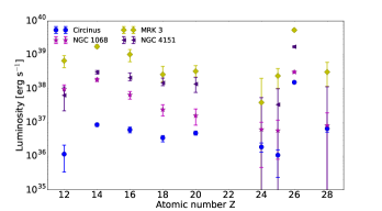
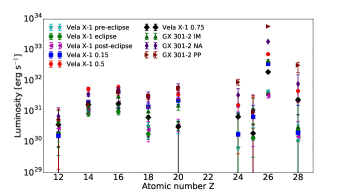
Figure 1: Luminosity of K$\alpha$ fluorescence lines corrected for Galactic absorption. Top: AGN. Bottom: XRB. Note the similar trends in AGN despite the disparity in luminosity and the phase dependence in the XRB.

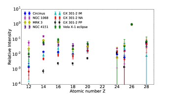
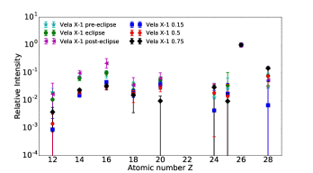
Figure 2: K$\alpha$ fluorescence line fluxes plotted relative to the flux of the Fe line. The Fe line is by far the strongest by 1 to 3 orders of magnitude depending on the source. Top: The source sample with a single Vela X-1 observation. The intensities do not, by themselves, reveal an inherent distinction between AGN and XRB. Bottom: All Vela X-1 epochs studied in this paper, suggesting a connection between line ratios and orbital phase.

4 Model for X-ray Fluorescence

When a dense neutral medium is illuminated by an X-ray source the various elements in the medium may be excited and produce X-ray fluorescence. The fluorescence from each element in each layer in the medium is proportional to the intensity of radiation reaching that layer.

The following derivation was adapted from Thomsen (2007). In a plane parallel approximation the incident photon-intensity $I(E,x)$ at energy $E$ and depth $x$ into the medium is:

$$I(E,x)=I(E,0)e^{-\tau(E,x)}$$ (1)

where $\tau(E,x)$ is the total optical depth a distance of $x$ into the medium, given by:

$$\tau(E,x)=\int_{0}^{x}\sigma(E)n_{\textrm{H}}dx=\sigma(E)N_{\textrm{H}}$$ (2)

where $\sigma(E)$ is the abundance-weighted average photo-ionization cross section per H atom, $n_{\textrm{H}}$ is the hydrogen number density, and $N_{\textrm{H}}$ is the hydrogen column density.

The K-shell ionization probability of a specific neutral element $Z$ by incident radiation at depth $x$ is:

$$d\tau_{Z,K}=\sigma_{Z,K}(E)n_{\textrm{Z}}dx=A_{\textrm{Z}}\sigma_{Z,K}(E)n_{\textrm{H}}dx$$ (3)

where $\sigma_{Z,K}$ is the K-shell ionization cross section of element $Z$, $A_{\textrm{Z}}$ is the elemental abundance (assumed to be solar, Asplund et al., 2009), and $n_{\textrm{Z}}=A_{\textrm{Z}}n_{\textrm{H}}$ is the number density of element $Z$. Thus, the intensity decrement due to K-shell ionization by an element $Z$ at a depth of $x$ in the medium is given by:

$$\frac{dI}{dx}=\int_{E_{K,Z}}^{\infty}I(E,0)e^{-\tau(E,x)}A_{\textrm{Z}}n_{\textrm{H}}\sigma_{Z,K}(E)dE$$ (4)

where $E_{K,Z}$ is the energy of the K-edge.

After a K-shell electron is released the ion can decay mainly through K$\alpha$ fluorescence, namely a 1s-2p transition. The probability for K$\alpha$ fluorescence is a factor of the fluorescence yield, $\omega_{K}$, and the probability of a 1s-2p transition over a 1s-3p transition. Higher order transitions are relevant only for heavy elements ($Z\geq 31$). This effective fluorescence yield, $\omega_{K\alpha}$, is given by:

$$\omega_{K\alpha}=\omega_{K}\frac{I_{K\alpha}}{I_{K\alpha}+I_{K\beta}}$$ (5)

Values of $\omega_{K}$ range from $\sim 0.03$ for Mg to $\sim 0.42$ for Ni. The branching ratio for K$\alpha$ over K$\beta$ emission varies from $\sim 1$ for Mg to $\sim 0.9$ for Ni. For $\omega_{K}$ we adopt the values from Hubbell et al. (1994) as they are consistent with experiments (Şahin et al., 2005) and more recent numerical calculations (Palmeri et al., 2012). For the branching ratio we adopt the values of Scofield (1972) to ensure all values are taken from the same source. Other values (Hölzer et al., 1997; Şahin et al., 2005; Palmeri et al., 2012) can change $\omega_{K\alpha}$ by $\sim 2\%$ at most, which is negligible relative to the line flux uncertainties (Tables 7,8,9). As noted by Palmeri et al. (2003), the branching ratio decreases with ionization. The ionization uncertainty affects $\omega_{K\alpha}$ more than that of the atomic data, but is still smaller than the measurement uncertainties.

Finally, to reach us, the emitted fluorescence photon must escape the medium. The resulting attenuation is given by the optical depth out of the medium at the energy of the K$\alpha$ line, $\tau(E_{K\alpha,Z},x)$. The observed intensity of the fluorescence line from the entire medium up to $x_{\textrm{tot}}$ is:

$$I_{f}=\int\displaylimits_{E_{K,Z}}^{\infty}\int\displaylimits_{0}^{x_{\textrm{tot}}}I(E,0)e^{-\tau(E,x)-\tau(E_{K\alpha,Z},x)}A_{\textrm{Z}}n_{\textrm{H}}\omega_{K\alpha}\sigma_{Z,K}(E)dxdE$$ (6)

Solving the integral over $x$ yields:

$$I_{f}=A_{\textrm{Z}}\omega_{K\alpha}\int\displaylimits_{E_{K,Z}}^{\infty}\frac{I(E,0)\sigma_{Z,K}(E)}{\sigma(E)+\sigma(E_{K\alpha,Z})}(1-e^{-\tau(E)-\tau(E_{K\alpha,Z})})dE$$ (7)

where $\tau(E_{K\alpha,Z})\equiv\tau(E_{K\alpha,Z},x_{\textrm{tot}})$ is the optical depth of the medium at the K$\alpha$ line and $\tau(E)\equiv\tau(E,x_{\textrm{tot}})$ is the total optical depth of the medium. In this equation, the factors most dependent on element are $A_{Z}$ and $\omega_{K\alpha}$ (see Table 1).

Two approximations for Equation (7) can be used. First, we consider an optically thin medium. In this case $1-e^{-\tau(E)-\tau(E_{K\alpha,Z})}\approx\tau(E)+\tau(E_{K\alpha,Z})$. Since $\tau=\sigma N_{\textrm{H}}$ Equation (7) now scales linearly with $N_{\textrm{H}}$:

$$I_{f}^{thin}=A_{\textrm{Z}}\omega_{K\alpha}N_{\textrm{H}}\int_{E_{K,Z}}^{\infty}I(E,0)\sigma_{Z,K}(E)dE$$ (8)

We assume a power-law ionizing spectrum of the form $I(E,0)=I_{0}(E/E_{0})^{-\Gamma}$ and a power-law dependence of $\sigma_{Z,K}(E)=\sigma_{Z,K}(E_{K,Z})(E/E_{K,Z})^{-2.65}$ (Yaqoob et al., 2001) to get:

$$I_{f}^{thin}=\frac{1}{\Gamma+1.65}I_{0}E_{0}^{\Gamma}A_{\textrm{Z}}\omega_{K\alpha}N_{\textrm{H}}E_{k,Z}^{1-\Gamma}\sigma_{Z,K}(E_{k,Z})$$ (9)

The second approximation of Equation (7) is for an optically thick medium, i.e. both $\tau(E)\rightarrow\infty$ and $\tau(E_{K\alpha,Z})\rightarrow\infty$:

$$I_{f}^{thick}=A_{\textrm{Z}}\omega_{K\alpha}\int\displaylimits_{E_{K,Z}}^{\infty}\frac{I_{0}(\frac{E}{E_{0}})^{-\Gamma}\sigma_{Z,K}(E)}{\sigma(E)+\sigma(E_{K\alpha,Z})}dE$$ (10)

This approximation turns out to be the model of reference for fluorescence lines in most astrophysical sources. The relative K$\alpha$ line intensities predicted by Equation (10) are listed in Table  1. The values for the abundances $A_{Z}$ and fluorescence yields $\omega_{K\alpha}$, which drive these intensities, are also given. It can be seen that the next strongest line after Fe K$\alpha$ is Si K$\alpha$, which is expected to be $\sim 10\%$ of the intensity of the Fe line.

Table 1: Canonical $I_{f}^{thick}$ intensities of X-ray fluorescence lines relative to Fe K$\alpha$.

Element	$\omega_{K\alpha}$	Solar Abundance	Relative Intensity
Mg	0.0291	$3.98\times 10^{-5}$	$0.067$
Si	0.0495	$3.24\times 10^{-5}$	$0.104$
S	0.0768	$1.32\times 10^{-5}$	$0.069$
Ar	0.1108	$2.51\times 10^{-6}$	$0.021$
Ca	0.1525	$2.19\times 10^{-6}$	$0.029$
Ti	0.2026	$8.91\times 10^{-8}$	$0.002$
Cr	0.2587	$4.37\times 10^{-7}$	$0.012$
Mn	0.2870	$2.69\times 10^{-7}$	$0.008$
Fe	0.3164	$3.16\times 10^{-5}$	$1$
Ni	0.3752	$1.66\times 10^{-6}$	$0.043$

A comparison between the approximations and the model for various column densities appear in Figure 3, as well as a comparison between different power-law profiles. Figure 3 shows that dramatic changes in the power law index are required to significantly change the line ratios. Note that the effect of a steep power-law is similar to that of an optically thin medium. In both cases there is a lack of hard-photon excitations.

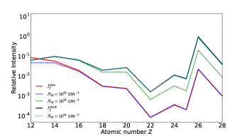
Figure 3: Top: Relative flux of K$\alpha$ fluorescence lines originating from different column densities of the fluorescing medium (Equation (7)). All models are plotted relative to the Fe line of $I_{f}^{thick}$. $I_{f}^{thin}$ (Equation (9)) agrees well with Equation (7) for $N_{\textrm{H}}=10^{22}$ cm^-2, except for Mg where $\tau(E_{K,Mg})\ll 1$ no longer holds. $I_{f}^{thick}$ (Equation (10)) is valid for $N_{\textrm{H}}\approx 10^{24}$ cm^-2 for all elements, and for Mg, Si, and S already at $N_{\textrm{H}}\approx 10^{23}$ cm^-2, since heavier elements emit from deeper within the medium.
Bottom: $I_{f}^{thick}$ for different power-law indices (Equation (10)). All models are plotted relative to the Fe line of the $\Gamma=2$ model. A steeper power-law causes less ionization of high-Z elements and thus higher ratio of the low-$Z$ ($Z<26$) lines to the Fe line, and vice versa.

5 Results

5.1 Comparison to theory

The prevailing hypothesis assumes AGN to be surrounded by dense obscuring material. Some XRB, such as GX 301-2, also show significant obscuration. Such an environment calls for the approximation of an optically thick fluorescing medium. Therefore, we first compare the measured fluxes with $I_{f}^{thick}$ described in Equation 10. Figure 4 shows a comparison between the measurements and theory for three values of $\Gamma$. As can be seen, the effects of the power-law slope are moderate compared to the spread in the data.

From the graph we see that the measurements from NGC 1068, MRK 3, and NGC 4151 are well described by Equation (10). Fluorescence lines from M51 (Xu et al., 2015), though not measured with gratings, show a similar trend. The nominal ratios imply the line-of-sight towards the fluorescing medium, as opposed to that towards the Seyfert 2 nucleus, is unobstructed. Vela X-1 also shows a decent agreement with $I_{f}^{thick}$, which implies that the observed fluxes may be explained by reflection from a high $N_{\textrm{H}}$ wind. This is in contrast to Sako et al. (1999) who assumed reflection from a low $N_{\textrm{H}}$ stellar wind, which caused the deduced $N_{\textrm{H}}$ values to increase with $Z$.

Unlike the other sources, Circinus and GX 301-2 show a systematic discrepancy of all low-Z elements with theoretical values of $I_{f}^{thick}$. The following sections will attempt to provide an explanation to this discrepancy.

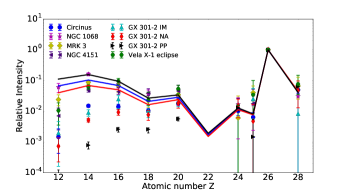
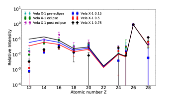
Figure 4: Relative flux of K$\alpha$ fluorescence lines (data points) compared to $I_{f}^{thick}$ (Equation (10)) with various power-law slopes: $\Gamma=2.3$, $\Gamma=2$ and $\Gamma=1.7$ as black, blue and red lines respectively (see Figure 3). Fluxes are plotted relative to the Fe line. Top: The present source sample with a single Vela X-1 epoch. The relative intensities of NGC 1068, Mrk 3, NGC 4151, and Vela X-1 eclipse follow the $I_{f}^{thick}$ ratios, while those of GX 301-2 and Circinus show significant deficiency in the low-$Z$ lines. Bottom: All Vela X-1 epochs studied in this paper. Notice the deficiency in Mg, Si, and S line fluxes in non-eclipse observations relative to $I_{f}^{thick}$.

5.2 Resonant Auger Destruction

Sako et al. (1999) proposed that Auger destruction may have a significant effect on fluorescence lines in Vela X-1 (see Section 1). A later theoretical analysis done by Liedahl (2005) showed the process to be complex and highly dependent on the ionization and excitation state of each element. Indeed, K$\alpha$ lines of L-shell Si in a laboratory photo-ionized plasma experiment showed no evidence of resonant Auger destruction (Loisel et al., 2017). Despite the complexity, several restrictions are immediately evident. First, K$\alpha$ Auger destruction cannot occur in a neutral medium as it requires an L-shell vacancy. Hence, higher Z elements require higher ionization for K$\alpha$ photo-excitation to occur. K$\beta$, in contrast, can be quenched by Auger destruction in lower charge states. Additionally, the energy difference between the K$\alpha$ energy of different L-shell Si ions is $\gtrsim 10$ eV. Thus, the velocity shear required to kinematically mix neighboring ions needs to be $\sim 1500$ km s^-1, which is not observed.

In a partially ionized medium, the ions may act as resonant absorbers for the emitted K$\alpha$ lines. Since $\omega_{K\alpha}\ll 1$, we can approximate the resulting Auger destruction as restricting our line of sight into the medium up to a photo-excitation optical depth of unity, $\tau^{PE}=1$. The absorption cross section at the center of a resonant line under assumption of a Gaussian line profile is:

$$\sigma^{PE}=\frac{\pi e^{2}f}{m_{e}c\sqrt{2\pi}\Delta\nu}$$ (11)

where $e$ is the electron charge, $m_{e}$ is the mass of the electron, $c$ is the speed of light, $f$ is the oscillator strength and $\Delta\nu$ is the Doppler width (standard deviation). We assume $\Delta\nu/\nu$ = 0.001, which is just under the HETG resolving power.

The column density of an element $Z$ for an optical depth $\tau^{PE}=N_{\textrm{Z}}\sigma^{PE}=1$ is:

$$N_{\textrm{Z}}=\frac{m_{e}c\sqrt{2\pi}\Delta\nu}{\pi e^{2}f}$$ (12)

Since $N_{\textrm{Z}}=A_{\textrm{Z}}N_{\textrm{H}}$, the corresponding $N_{\textrm{H}}$ for abundant elements is smaller than for rare elements. Consequently, for abundant elements $N_{\textrm{H}}<10^{22}$ cm^-2 and thus $\tau(E)\ll\tau^{PE}=1$. We can therefore use Equation (9) to get $I_{f}^{thin}$ in the case of dominant Auger destruction:

$$I_{f}^{thin}=\frac{1}{\Gamma+1.65}I_{0}E_{0}^{\Gamma}\omega_{K\alpha}\frac{m_{e}c\sqrt{2\pi}\Delta\nu}{\pi e^{2}f}E_{K,Z}^{1-\Gamma}\sigma_{Z,K}(E_{K,Z})$$ (13)

Equation (13) is independent of $A_{\textrm{Z}}$, so all abundant elements will have similar $I_{f}^{thin}$. For the rarer elements $\tau(E)\ll\tau^{PE}=1$ no longer holds. Thus, we must use the accurate expression (Equation 7 with the corresponding $N_{\textrm{H}}$).

Another possible approximation is for Auger destruction in an optically thick medium. We assume the cross section for resonant absorption to be $\sigma_{eff,Z}=(1-\omega_{K\alpha,Z})\sigma_{Z}^{PE}$, effectively assuming the scattering is destructive with probability $(1-\omega_{K\alpha,Z})$. This approximation effectively adds $A_{Z}\sigma_{eff,Z}$ to the denominator of Eq (10), which yields similar results to Equation (7) with the $N_{\textrm{H}}$ corresponding to Equation (12).

Both approximations are shown in Figure 5, neither of which produces a good agreement with any observation. Selective Auger destruction could explain the low-Z relative intensities of Circinus, if somehow Fe is unaffected. The K$\beta$/K$\alpha$ nominal ratios presented in Sec. 3.2 (e.g., 0.14 for Circinus) further argue against a significant role of Auger destruction, which is discussed in Section 6.

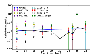
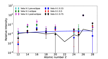
Figure 5: Relative flux of K$\alpha$ fluorescence lines compared to theoretical ratios predicted by Auger destruction models. The blue line describes $I_{f}^{thin}$ where the optical depth is limited by photo-excitation (Equation (13)). The black line describes $I_{f}^{thick}$, but with Auger resonant scattering factored in. All models are normalized relative to the theoretical Fe line flux of $I_{f}^{thick}$ (Equation (10)).

5.3 Excess Line of Sight Column Density

We propose a simple explanation to the relatively weak low-$Z$ lines observed in several of the present measurements. The deficiency of the low-Z relative intensities with respect to $I_{f}^{thick}$ (Figure 4) decreases with Z. Therefore, excess line of sight column density beyond the Galactic column could explain the anomalous ratios. If correct, a single column density value $N_{\textrm{H}}^{ex}$ for each object would need to explain the quenching of the fluorescence lines of all low-Z elements. We can then use the measured fluxes to estimate $N_{\textrm{H}}^{ex}$ self-consistently for each object. The observed intensity ratio with an additional column density $N_{\textrm{H}}^{ex}$ would be:

$$\frac{I_{f,Z}^{obs}}{I_{f,Fe}^{obs}}=\frac{I_{f,Z}^{thick}e^{-\sigma(E_{K,Z})N_{\textrm{H}}^{ex}}}{I_{f,Fe}^{thick}e^{-\sigma(E_{K,Fe})N_{\textrm{H}}^{ex}}}$$ (14)

Thus we can extract $N_{\textrm{H}}^{ex}$ for each element:

$$N_{\textrm{H}}^{ex}=\frac{1}{\sigma(E_{K,Fe})-\sigma(E_{K,Z})}\ln\left(\frac{I_{f,Z}^{obs}}{I_{f,Fe}^{obs}}\frac{I_{f,Fe}^{thick}}{I_{f,Z}^{thick}}\right)$$ (15)

$N_{\textrm{H}}^{ex}$ as derived by Si K$\alpha$ is the most reliable estimate, as it is the best measured line except for Fe K$\alpha$, and their cross section difference is the second highest. For Si Equation (15) gives:

$$N_{\textrm{H}}^{ex}(\textrm{Si})=2.42\times 10^{22}\ln\left(0.104\frac{I_{f,Fe}^{obs}}{I_{f,Si}^{obs}}\right)$$ (16)

In extra-galactic sources excess column density can be associated with dust extinction and reddening. In NGC 1068 the above line ratios show only marginal evidence for $N_{\textrm{H}}^{ex}$, which is consistent with the low reddening towards the narrow line region of NGC 1068 ($A_{V}<0.15$, Crenshaw & Kraemer, 2000). In Mrk 3 only Mg and Si K$\alpha$ require marginal excess column density of $N_{\textrm{H}}^{ex}(\textrm{Mg})=1.1^{+0.3}_{-0.6}\times 10^{22}$ cm^-2 and $N_{\textrm{H}}^{ex}(\textrm{Si})=0.4\pm 0.3\times 10^{22}$ cm^-2 respectively, while other elements provide only an upper limit of $N_{\textrm{H}}^{ex}<2\times 10^{22}$ cm^-2. This value is consistent with the reddening based estimate of Collins et al. (2005) of $N_{\textrm{H}}\sim 10^{21}$ cm^-2 .

In the NGC 4151 combined 2014 observations the K$\alpha$ intensity ratios of Mg, Si and S to Fe predict a column density of $N_{\textrm{H}}^{ex}\sim 2\times 10^{22}$ cm^-2. The $N_{\textrm{H}}^{ex}$ corrected relative intensities are plotted in Figure 6 (top panel). Note that Ar and Ca K$\alpha$ intensity ratios are slightly higher than canonical values and therefore require no $N_{\textrm{H}}^{ex}$. This result is consistent with the two other observations. Since NGC 4151 does not show significant reddening towards the narrow line region (Kraemer et al., 2000), the varying outflow may be responsible for $N_{\textrm{H}}^{ex}$.

In contrast to the other AGN, the Circinus galaxy requires significant $N_{\textrm{H}}^{ex}$ (Figure 4). The results are listed in Table 2 and show a general agreement with each other. If we assume $\Gamma=1.8$ instead of $\Gamma=2.0$, the insignificant increasing trend vanishes. We find $N_{\textrm{H}}^{ex}(\textrm{Si})=(4.7\pm 0.3)\times 10^{22}$ cm^-2, or $(4.0\pm 0.3)\times 10^{22}$ cm^-2 for $\Gamma=1.8$, which is in excellent agreement with dust extinction measurements in Circinus. Tristram et al. (2007) estimated the extinction in Circinus galactic foreground to be $A_{V}=20$ magnitudes which corresponds to a column density of $N_{\textrm{H}}\approx 4\times 10^{22}$ cm^-2, assuming $N_{\textrm{H}}\approx 2A_{V}\times 10^{21}$ cm^-2. The $N_{\textrm{H}}^{ex}$ corrected relative intensities are plotted in Figure 6 (top panel) and match those predicted by $I_{f}^{thick}$ well.

We note that $N_{\textrm{H}}>10^{24}$ cm^-2 is the default assumption of the different AGN tori models. To fit Seyfert 2 X-ray spectra, these models require the torus to be clumpy to create unobscured lines of sight (Yaqoob, 2012). Totally unobscured cases where the Si/Fe K$\alpha$ intensity ratio is $\sim 0.1$, such as in NGC 1068, are therefore difficult to explain under these assumptions (Liu et al., 2016). The moderate $N_{\textrm{H}}^{ex}$ values found above for all AGN are well below the Compton-thick column of the torus.

The situation for Vela X-1 is complicated and phase dependent. In the near eclipse observations (Eclipse, Pre and Post) deviations from $I_{f}^{thick}$ initially appears minor, whereas the other observations require significant $N_{\textrm{H}}^{ex}$ corrections. This inconsistency hints at a more complex explanation. Following Sako et al. (1999), the fluorescing medium near eclipse is likely not optically thick and therefore not well described by $I_{f}^{thick}$. Thus, we must calculate excess column density based on the full model (Equation (7)) rather than on $I_{f}^{thick}$ (Equation (10)). Table 3 lists $N_{\textrm{H}}^{ex}$ for the near eclipse Vela X-1 observations using a fluorescing medium of $N_{\textrm{H}}=2\times 10^{23}$ cm^-2. Table 4 lists $N_{\textrm{H}}^{ex}$ for Vela X-1 phases 0.75, 0.5 and 0.15, calculated based on $I_{f}^{thick}$. As evident in the tables, a total line of sight column density (interstellar and excess) of $N_{\textrm{H}}^{tot}=4.0\pm 0.5\times 10^{22}$ cm^-2 is roughly consistent across phases and elements. In Figure 6 (bottom panel) we present the relative intensities for Vela X-1 observations with $N_{\textrm{H}}^{tot}=4\times 10^{22}$ cm^-2.

The most significant deviation from the $I_{f}^{thick}$ approximation is in GX 301-2, with each epoch requiring a different $N_{\textrm{H}}^{ex}$. The results are presented in Table 5. Note that the Galactic $N_{\textrm{H}}$ towards GX 301-2 is already high at $N_{\textrm{H}}=1.42\times 10^{22}$ cm^-2. The estimates for $N_{\textrm{H}}^{ex}$ for the IM and NA observations are each roughly consistent between elements. At the IM phase $N_{\textrm{H}}^{ex}(\textrm{Si})=(5.9\pm 0.6)\times 10^{22}$ cm^-2 and at the NA phase $N_{\textrm{H}}^{ex}(\textrm{Si})=(7.2\pm 0.2)\times 10^{22}$ cm^-2, which is consistent with MAXI measurements of total $N_{\textrm{H}}\lesssim 10^{23}$ cm^-2 and $N_{\textrm{H}}\approx 12\pm 4\times 10^{22}$ cm^-2 for the IM and NA phases respectively (Islam & Paul, 2014, Figure 5 therein).

The $N_{\textrm{H}}^{ex}$ values for the PP observation are higher (reaching $3\times 10^{23}$ cm^-2), as expected for an XRB near periastron and as measured by Islam & Paul (2014). These measurements show a trend of $N_{\textrm{H}}^{ex}$ increasing with $Z$. A possible way to remedy this inconsistency is with a flat power-law slope of $\Gamma<1$. Indeed, $\Gamma<1$ slopes were measured by Islam & Paul (2014) around the PP phase.

To summarize, Figure 6 shows relative intensities after correcting for $N_{\textrm{H}}^{ex}(\textrm{Si})$ in Circinus, GX 301-2 and Vela X-1. The overall agreement between the data and the models is significantly improved over that of Figure 4.

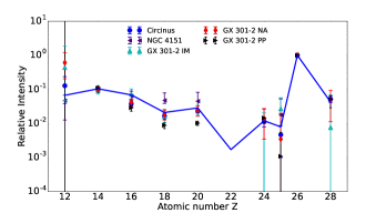
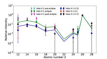
Figure 6: Relative flux of K$\alpha$ fluorescence lines compared to theoretical values after $N_{\textrm{H}}^{ex}(\textrm{Si})$ corrections. All fluxes are normalized relative to the flux of the Fe line. The blue line represents $I_{f}^{thick}$ (Equation (10)). Top: The correction works particularly well for Circinus and the GX 301-2 IM and NA phases and less for the PP phase. Bottom: The correction works well for the Vela X-1 non-eclipse phases. For the eclipse phases a model of a fluorescing medium with $N_{\textrm{H}}=2\times 10^{23}$ cm^-2 is required (Equation (7), green line).

.

Table 2: Line of sight excess column density ($N_{\textrm{H}}^{ex}$, Equation (15)) for the Circinus Galaxy and for the NGC 4151 combined observation.

Element	Circinus Galaxy $N_{\textrm{H}}^{ex}$ $(10^{22}$ cm${}^{-2})$	NGC 4151 $N_{\textrm{H}}^{ex}$ $(10^{22}$ cm${}^{-2})$
Mg	$4.1\pm 0.8$	$2.4\pm 0.7$
Si	$4.7\pm 0.3$	$1.9\pm 0.3$
S	$7.9\pm 0.9$	$2.3\pm 1.4$
Ar	$7.0\pm 2.0$	-
Ca	$9.8\pm 2.8$	-

Table 3: Line of sight excess column density ($N_{\textrm{H}}^{ex}$, Equation (15)) for the Vela X-1 eclipse, pre-eclipse and post-eclipse phases, estimated based on Equation (7) with $N_{\textrm{H}}=2\times 10^{23}$ cm^-2.

Element	Vela X-1(Eclipse) $N_{\textrm{H}}^{ex}$ $(10^{22}$ cm${}^{-2})$	Vela X-1(Pre) $N_{\textrm{H}}^{ex}$ $(10^{22}$ cm${}^{-2})$	Vela X-1(Post) $N_{\textrm{H}}^{ex}$ $(10^{22}$ cm${}^{-2})$
Mg	$3.0\pm 0.8$	$2.4\pm 0.6$	$2.5\pm 1.3$
Si	$3.6\pm 0.4$	$3.5\pm 0.5$	$2.6\pm 0.6$
S	$3.2\pm 1.1$	$2.9\pm 1.3$	$<1.1$
Ar	$8.3\pm 5.7$	$<8.6$	$<11.3$
Ca	$<10.0$	$<17.9$	$<10.1$

Table 4: Line of sight excess column density ($N_{\textrm{H}}^{ex}$, Equation (15)) for Vela X-1 phases 0.5, 0.75 and 0.15, estimated based on $I_{f}^{thick}$ (Equation (10)).

Element	Vela X-1(0.5) $N_{\textrm{H}}^{ex}$ $(10^{22}$ cm${}^{-2})$	Vela X-1(0.75) $N_{\textrm{H}}^{ex}$ $(10^{22}$ cm${}^{-2})$	Vela X-1(0.15) $N_{\textrm{H}}^{ex}$ $(10^{22}$ cm${}^{-2})$
Mg	$4.1\pm 1.1$	$3.1\pm 0.8$	$4.6\pm 1.3$
Si	$4\pm 0.3$	$3.6\pm 0.5$	$4.7\pm 0.4$
S	$4.2\pm 1$	$3.7\pm 1.4$	$2.1\pm 0.7$
Ar	$<5.7$	$<11.0$	$<4.4$
Ca	$<6.5$	$-$	$-$

Table 5: Line of sight excess column density ($N_{\textrm{H}}^{ex}$, Equation (15)) for GX 301-2.

Element	GX 301-2(IM) $N_{\textrm{H}}^{ex}$ $(10^{22}$ cm${}^{-2})$	GX 301-2(NA) $N_{\textrm{H}}^{ex}$ $(10^{22}$ cm${}^{-2})$	GX 301-2 (PP) $N_{\textrm{H}}^{ex}$ $(10^{22}$ cm${}^{-2})$
Mg	$3.7\pm 1.2$	$4.8\pm 0.8$	$-$
Si	$5.9\pm 0.6$	$7.3\pm 0.3$	$11.9\pm 0.6$
S	$5.1\pm 2$	$9.9\pm 1.0$	$16.2\pm 0.8$
Ar	$6.9\pm 4.3$	$10.0\pm 3.6$	$20.9\pm 1.8$
Ca	$7.3\pm 6.9$	$9.5\pm 7.0$	$34.5\pm 3.0$

6 Discussion

Excess line of sight column density creates good agreement between the simple plane parallel models presented in Section 4 and the data across many independent targets and observations. Any minor remaining discrepancies between the data and models can be interpreted as variations in the few model assumption: ionizing spectrum, fluorescing medium $N_{\textrm{H}}$, and elemental abundances. Such examples are shown above for Vela X-1 ($N_{\textrm{H}}$) and GX 301-2 ($\Gamma$). Additionally, a more complex geometry may involve illumination-incidence and line-of-sight angles, which have a minor effect on the relative line intensities of Equation (10). An optimal fit obtained by varying all parameters is beyond the scope of the present work.

Special care should also be taken when interpreting results from the Si K$\alpha$ measurement, where we accounted for the blend with the H-like Mg Ly$\beta$ (Section 3.1). In our calculations, we assumed $N_{\textrm{H}}^{ex}$ to affect only the fluorescence lines. In practice, this implies the near-neutral and ionized sources may have different line of sight column densities. This result is supported by the GX 301-2 observations, where the ionized emission lines are more obscured than the fluorescence lines. In fact, the He-like Si lines at $\sim 6.7$ Å are already absorbed out of the spectrum, whereas the Si K$\alpha$ is clearly visible at a longer wavelength.

Figure 5 shows that Auger destruction cannot explain the observed line intensities, as it needs to selectively destroy only florescence from low-Z elements. Selective Auger destruction might be possible if L-shell vacancies exist in low-Z elements, but not in higher Z elements. This requirement limits the ionization parameter $\xi$ to a narrow range. Based on Kallman & Bautista (2001), this range for selective Auger destruction up to and including Ca is $1.2<\log(\xi)<1.7$, making this model restricted, but not impossible. The main problem; however, with Auger destruction stems from the observation of the nominal Fe K$\beta$ line intensity. With selective Auger destruction, we would expect a decrease in the K$\beta$/K$\alpha$ line intensity ratio (Liedahl, 2005), which is not observed in any of the present spectra (see Section 3.2).

7 Conclusions

The present work can be summarized as follows:

• We surveyed the Chandra/HETG archive for all grating spectra that feature at least four X-ray K$\alpha$ fluorescence lines in AGN and in Galactic XRB.

• The K$\alpha$ intensity ratios between elements follow similar trends in most observations, except for a few cases in which the low-Z lines (e.g., Mg, Si) are reduced by orders of magnitude (Figures 1,2).

• For the most part, the relative K$\alpha$ intensities follow a simple plane-parallel approximation of a dense, near-neutral optically-thick medium, defined as $I_{f}^{thick}$ in Equation (10). The only two (sets of) free parameters in this model are the ionizing spectrum and the elemental abundances (Figure 3).

• The reduced K$\alpha$ intensities in the low-Z elements is explained satisfactorily and self-consistently by excess column density along the line of sight (Equation (15) and Figure 6). This excess column derived here from the K$\alpha$ fluorescence line ratios is nicely corroborated by independent measurements, primarily reddening in AGN, and X-ray continuum absorption in XRB. Hence, X-ray fluorescence line ratios can provide an independent estimate of interstellar column density.

• The K$\alpha$ intensity ratios do not show evidence for resonant Auger destruction. Furthermore, the K$\beta$/K$\alpha$ intensity ratios are nominal, or even enhanced, in all sources. This further indicates the K$\alpha$ fluorescing medium is near neutral.

Appendix A Data and measurements

Table 6: List of observations used

Object	Observation ID	Date observed	Exposure (s)	Notes
Circinus Galaxy	374	2000-06-15	7118
Circinus Galaxy	62877	2000-06-16	60220
Circinus Galaxy	4770	2004-06-02	55030
Circinus Galaxy	4771	2004-11-28	58970
Circinus Galaxy	10226	2008-12-08	19670
Circinus Galaxy	10223	2008-12-15	102900
Circinus Galaxy	10832	2008-12-19	20610
Circinus Galaxy	10833	2008-12-22	28360
Circinus Galaxy	10224	2008-12-23	77100
Circinus Galaxy	10844	2008-12-24	27170
Circinus Galaxy	10225	2008-12-26	67890
Circinus Galaxy	10842	2008-12-27	36740
Circinus Galaxy	10843	2008-12-29	57010
Circinus Galaxy	10873	2009-03-01	18100
Circinus Galaxy	10850	2009-03-03	13850
Circinus Galaxy	10872	2009-03-04	16530
NGC 1068	332	2000-12-04	45700
NGC 1068	9148	2008-12-05	79540
NGC 1068	9149	2008-11-19	88730
NGC 1068	9150	2008-11-27	41080
NGC 1068	10815	2008-11-20	19070
NGC 1068	10816	2008-11-18	16160
NGC 1068	10817	2008-11-22	32650
NGC 1068	10823	2008-11-25	34540
NGC 1068	10829	2008-11-30	38440
NGC 1068	10830	2008-12-03	42900
MRK 3	873	2000-03-18	100600
MRK 3	12874	2011-04-19	77060
MRK 3	12875	2011-04-25	29860
MRK 3	13264	201-04-27	35760
MRK 3	13263	2011-04-28	19720
MRK 3	13261	2011-05-02	22080
MRK 3	13406	2011-05-03	21430
MRK 3	13254	2011-08-26	31530
MRK 3	14331	2011-08-28	51210
NGC 4151	335	2000-03-05	47440
NGC 4151	7829	2007-03-19	49230
NGC 4151	16089	2014-02-12	171900
NGC 4151	16090	2014-03-08	68870
GX 301-2	103	2000-06-19	39519	0.167-179 (IM)
GX 301-2	2733	2002-01-13	39230	0.97-0.982 (PP)
GX 301-2	3433	2002-02-03	59030	0.48-0.497 (NA)
Vela X-1	102	2000-04-13	28010	0.015-0.051 : post-eclipse (Post)
Vela X-1	1926	2001-02-11	83150	0.980 - 0.093 : eclipse
Vela X-1	1927	2001-02-07	29430	0.481-0.522 : 0.5
Vela X-1	14654	2013-07-30	45880	0.748-0.807 : 0.75
Vela X-1	18617	2017-02-21	44180	0.936-0.993 : pre-eclipse (Pre)
Vela X-1	19953	2017-02-22	70470	0.132-0.223 : 0.15

Table 7: Vela X-1 measured fluorescence line fluxes at various orbital phases

Element	Rest Frame	Photon Flux ($10^{-6}$ ph s-1 cm -2)
	Wavelength (Å)	Eclipse	Pre-Eclipse	Post-Eclipse	0.5	0.75	0.15
Mg	9.890	$1.9^{+1.5}_{-1.3}$	$4.2^{+1.6}_{-3.2}$	$<6.7$	$5.1^{+6.0}_{-5.0}$	$3.5^{+2.3}_{-2.9}$	$<3.8$
Si	7.126	$11.2^{+1.9}_{-2.0}$	$13.9^{+2.8}_{-2.8}$	$15.3^{+3.7}_{-3.8}$	$71^{+10}_{-10}$	$21.9^{+4.3}_{-4.3}$	$26.3^{+4.1}_{-4.2}$
S	5.373	$17.1^{+3.7}_{-3.6}$	$21.7^{+2.8}_{-8.1}$	$35^{+16}_{-11}$	$105^{+21}_{-20}$	$30.9^{+8.9}_{-8.4}$	$77^{+11}_{-10}$
Ar	4.193	$4.8^{+3.4}_{-1.4}$	$7.6^{+2.8}_{-2.8}$	$5.7^{+4.9}_{-3.4}$	$63^{+17}_{-34}$	$14^{+11}_{-11}$	$32^{+10}_{-10}$
Ca	3.359	$9.6^{+3.0}_{-2.9}$	$9.3^{+4.5}_{-4.0}$	$9.9^{+5.9}_{-3.7}$	$100^{+30}_{-28}$	$<26$	$64^{+17}_{-16}$
Cr	2.290	$<2.8$	$<8.9$	$<6.5$	$66^{+66}_{-64}$	$<72$	$<39$
Mn	2.102	$6^{+12}_{-5}$	$<14$	$<3.2$	$<132$	$<62$	$<70$
Fe (K$\alpha$)	1.936	$178^{+17}_{-16}$	$216^{+28}_{-25}$	$160^{+28}_{-27}$	$3570^{+150}_{-150}$	$939^{+77}_{-75}$	$1720^{+70}_{-70}$
Fe (K$\beta$)	1.757	$23^{+39}_{-11}$	$49^{+22}_{-21}$	$<24$	$1070^{+230}_{-200}$	$139^{+123}_{-63}$	$368^{+105}_{-120}$
Ni	1.658	$14^{+13}_{-7}$	$<21$	$<27$	$260^{+230}_{-150}$	$135^{+96}_{-91}$	$<89$

Table 8: Measured fluorescence line fluxes for GX 301-2, Mrk 3, NGC 1068 and The Circinus Galaxy

Element	Rest Frame	Photon Flux ($10^{-6}$ ph s-1 cm -2)
	Wavelength (Å)	GX 301-2 IM	GX 301-2 NA	GX 301-2 PP	Circinus	Mrk 3	NGC 1068
Mg	9.890	$1.7^{+2.4}_{-1.6}$	$2.7^{+2.3}_{-1.9}$	$<1.4$	$0.5^{+0.4}_{-0.3}$	$1.2^{+0.5}_{-0.4}$	$3.0^{+1.0}_{-1.0}$
Si	7.126	$8.1^{+1.9}_{-1.9}$	$19.1^{+2.4}_{-2.6}$	$9.1^{+2.5}_{-2.2}$	$4.8^{+0.5}_{-0.5}$	$4.3^{+0.5}_{-0.5}$	$8.0^{+0.8}_{-0.9}$
S	5.373	$22^{+7}_{-11}$	$34^{+7}_{-8}$	$30.1^{+4.0}_{-6.0}$	$4.5^{+0.9}_{-0.8}$	$3.3^{+1.3}_{-1.3}$	$3.8^{+0.9}_{-1.0}$
Ar	4.193	$9.3^{+4.3}_{-3.7}$	$28^{+10}_{-10}$	$29.7^{+3.7}_{-7.1}$	$3.3^{+0.6}_{-0.8}$	$1.1^{+0.8}_{-0.4}$	$1.8^{+0.7}_{-0.6}$
Ca	3.359	$18^{+6}_{-5}$	$67^{+23}_{-21}$	$65^{+9}_{-9}$	$5.8^{+0.5}_{-0.5}$	$1.7^{+0.8}_{-0.5}$	$1.5^{+0.9}_{-0.7}$
Cr	2.290	$<15$	$57^{+34}_{-35}$	$150^{+32}_{-31}$	$3.3^{+1.0}_{-1.0}$	$<1.2$	$0.8^{+0.5}_{-0.8}$
Mn	2.102	$23^{+26}_{-18}$	$<62$	$<45$	$2.1^{+0.9}_{-1.6}$	$2.0^{+1.3}_{-1.1}$	$0.9^{+0.9}_{-0.7}$
Fe (K$\alpha$)	1.936	$883^{+59}_{-56}$	$3680^{+100}_{-100}$	$11470^{+270}_{-280}$	$319.7^{+3.2}_{-9.9}$	$48.4^{+3.9}_{-3.8}$	$49.5^{+3.5}_{-3.2}$
Fe (K$\beta$)	1.757	$199^{+81}_{-48}$	$765^{+135}_{-93}$	$3460^{+250}_{-210}$	$44.1^{+4.4}_{-4.0}$	$8.6^{+3.2}_{-2.8}$	$5.3^{+1.9}_{-2.5}$
Ni	1.658	$<64$	$180^{+180}_{-130}$	$730^{+170}_{-310}$	$15.9^{+3.8}_{-3.4}$	$3.2^{+3.0}_{-2.0}$	$<3.6$

Table 9: Measured fluorescence line fluxes for NGC 4151

Element	Rest Frame	Photon Flux ($10^{-6}$ ph s-1 cm -2)
	Wavelength (Å)	03-2000	03-2007	02-2014	03-2014
Mg	9.890	$<3.3$	$<2.1$	$2.8^{+1.2}_{-1.2}$	$1.7^{+1.8}_{-1.2}$
Si	7.126	$8.0^{+2.1}_{-2.2}$	$5.1^{+1.4}_{-1.9}$	$7.4^{+1.2}_{-1.2}$	$10.5^{+1.9}_{-2.1}$
S	5.373	$5.0^{+7.0}_{-3.4}$	$6.9^{+5.3}_{-2.5}$	$7.7^{+2.3}_{-2.2}$	$8.3^{+3.8}_{-3.2}$
Ar	4.193	$<14$	$6.8^{+3.8}_{-3.6}$	$8.4^{+4.0}_{-3.4}$	$<4.6$
Ca	3.359	$13^{+11}_{-9}$	$5.6^{+4.4}_{-3.5}$	$6.4^{+5.0}_{-4.0}$	$18^{+11}_{-9}$
Cr	2.290	$<490$	$8.9^{+8.3}_{-7.6}$	$<5.6$	$<10.2$
Mn	2.102	$<17$	$<4.0$	$<7.5$	$<22.3$
Fe (K$\alpha$)	1.936	$202^{+39}_{-28}$	$97^{+21}_{-18}$	$177^{+14}_{-14}$	$152^{+24}_{-22}$
Fe (K$\beta$)	1.757	$<37$	$17^{+17}_{-14}$	$32^{+13}_{-11}$	$19^{+28}_{-12}$
Ni	1.658	$29^{+32}_{-27}$	$26^{+21}_{-17}$	$12^{+11}_{-9}$	$<31$

References

- Arévalo et al. (2014) Arévalo, P., Bauer, F., Puccetti, S., et al. 2014, The Astrophysical Journal, 791, 81
- Arnaud (1996) Arnaud, K. 1996, in Astronomical Data Analysis Software and Systems V, Vol. 101, 17
- Asplund et al. (2009) Asplund, M., Grevesse, N., Sauval, A. J., & Scott, P. 2009, Annual Review of Astronomy and Astrophysics, 47, 481
- Bambynek et al. (1972) Bambynek, W., Crasemann, B., Fink, R., et al. 1972, Reviews of modern physics, 44, 716
- Bekhti et al. (2016) Bekhti, N. B., Flöer, L., Keller, R., et al. 2016, Astronomy & Astrophysics, 594, A116
- Belloni & Hasinger (1990) Belloni, T., & Hasinger, G. 1990, Astronomy and Astrophysics, 230, 103
- Bogdán et al. (2017) Bogdán, Á., Kraft, R. P., Evans, D. A., Andrade-Santos, F., & Forman, W. R. 2017, The Astrophysical Journal, 848, 61
- Collins et al. (2005) Collins, N. R., Kraemer, S. B., Crenshaw, D. M., et al. 2005, The Astrophysical Journal, 619, 116
- Couto et al. (2016) Couto, J., Kraemer, S., Turner, T., & Crenshaw, D. 2016, The Astrophysical Journal, 833, 191
- Crenshaw & Kraemer (2000) Crenshaw, D. M., & Kraemer, S. B. 2000, The Astrophysical Journal, 532, 247
- Dickey & Lockman (1990) Dickey, J. M., & Lockman, F. J. 1990, Annual review of astronomy and astrophysics, 28, 215
- Dopita et al. (2002) Dopita, M. A., Groves, B. A., Sutherland, R. S., Binette, L., & Cecil, G. 2002, The Astrophysical Journal, 572, 753
- Ferland et al. (2017) Ferland, G., Chatzikos, M., Guzmán, F., et al. 2017, Revista mexicana de astronomía y astrofísica, 53
- George & Fabian (1991) George, I., & Fabian, A. 1991, Monthly Notices of the Royal Astronomical Society, 249, 352
- Goldstein et al. (2004) Goldstein, G., Huenemoerder, D. P., & Blank, D. 2004, The Astronomical Journal, 127, 2310
- Hölzer et al. (1997) Hölzer, G., Fritsch, M., Deutsch, M., Härtwig, J., & Förster, E. 1997, Phys. Rev. A, 56, 4554
- Hubbell et al. (1994) Hubbell, J., Trehan, P., Singh, N., et al. 1994, Journal of Physical and Chemical Reference Data, 23, 339
- Huenemoerder et al. (2011) Huenemoerder, D. P., Mitschang, A., Dewey, D., et al. 2011, The Astronomical Journal, 141, 129
- Islam & Paul (2014) Islam, N., & Paul, B. 2014, Monthly Notices of the Royal Astronomical Society, 441, 2539
- Kalberla et al. (2005) Kalberla, P. M., Burton, W., Hartmann, D., et al. 2005, Astronomy & Astrophysics, 440, 775
- Kallman & Bautista (2001) Kallman, T., & Bautista, M. 2001, The Astrophysical Journal Supplement Series, 133, 221
- Kallman et al. (2013) Kallman, T., Evans, D. A., Marshall, H., et al. 2013, The Astrophysical Journal, 780, 121
- Kraemer et al. (2000) Kraemer, S., Crenshaw, D., Hutchings, J., et al. 2000, The Astrophysical Journal, 531, 278
- Kreykenbohm et al. (2008) Kreykenbohm, I., Wilms, J., Kretschmar, P., et al. 2008, Astronomy & Astrophysics, 492, 511
- Liedahl (2005) Liedahl, D. A. 2005in , American Institute of Physics, 99–108
- Liu et al. (2016) Liu, J., Liu, Y., Li, X., et al. 2016, Monthly Notices of the Royal Astronomical Society: Letters, 459, L100
- Loisel et al. (2017) Loisel, G. P., Bailey, J. E., Liedahl, D., et al. 2017, Physical Review Letters, 119, 075001
- Marinucci et al. (2013) Marinucci, A., Miniutti, G., Bianchi, S., Matt, G., & Risaliti, G. 2013, Monthly Notices of the Royal Astronomical Society, 436, 2500
- Miller et al. (2018) Miller, J., Cackett, E., Zoghbi, A., et al. 2018, The Astrophysical Journal, 865, 97
- Mukherjee & Paul (2004) Mukherjee, U., & Paul, B. 2004, Astronomy & Astrophysics, 427, 567
- Netzer (1996) Netzer, H. 1996, The Astrophysical Journal, 473, 781
- Ogle et al. (2003) Ogle, P., Brookings, T., Canizares, C., Lee, J., & Marshall, H. 2003, Astronomy & Astrophysics, 402, 849
- Ogle et al. (2000) Ogle, P., Marshall, H., Lee, J., & Canizares, C. 2000, The Astrophysical Journal Letters, 545, L81
- Palmeri et al. (2003) Palmeri, P., Mendoza, C., Kallman, T., Bautista, M., & Meléndez, M. 2003, Astronomy & Astrophysics, 410, 359
- Palmeri et al. (2012) Palmeri, P., Quinet, P., Mendoza, C., et al. 2012, Astronomy & Astrophysics, 543, A44
- Quaintrell et al. (2003) Quaintrell, H., Norton, A. J., Ash, T., et al. 2003, Astronomy & Astrophysics, 401, 313
- Ross et al. (1996) Ross, R. R., Fabian, A. C., & Brandt, W. N. 1996, MNRAS, 278, 1082
- Şahin et al. (2005) Şahin, M., Demir, L., & Budak, G. 2005, Applied radiation and isotopes, 63, 141
- Sako et al. (2000) Sako, M., Kahn, S. M., Paerels, F., & Liedahl, D. A. 2000, The Astrophysical Journal Letters, 543, L115
- Sako et al. (1999) Sako, M., Liedahl, D. A., Kahn, S. M., & Paerels, F. 1999, The Astrophysical Journal, 525, 921
- Sambruna et al. (2000) Sambruna, R. M., Netzer, H., Kaspi, S., et al. 2000, The Astrophysical Journal Letters, 546, L13
- Schulz et al. (2001) Schulz, N. S., Canizares, C. R., Lee, J. C., & Sako, M. 2001, The Astrophysical Journal Letters, 564, L21
- Scofield (1972) Scofield, J. H. 1972, THEORETICAL RADIATIVE TRANSITION RATES FOR K-AND L-SHELL X RAYS., Tech. rep., California Univ., Livermore. Lawrence Livermore Lab.
- Stern et al. (2014) Stern, J., Laor, A., & Baskin, A. 2014, Monthly Notices of the Royal Astronomical Society, 438, 901
- Thomsen (2007) Thomsen, V. 2007, Spectroscopy, 22, 46
- Tristram et al. (2007) Tristram, K., Meisenheimer, K., Jaffe, W., et al. 2007, Astronomy & Astrophysics, 474, 837
- Watanabe et al. (2003) Watanabe, S., Sako, M., Ishida, M., et al. 2003, The Astrophysical Journal Letters, 597, L37
- Watanabe et al. (2006) —. 2006, The Astrophysical Journal, 651, 421
- Xu et al. (2015) Xu, W., Liu, Z., Gou, L., & Liu, J. 2015, Monthly Notices of the Royal Astronomical Society: Letters, 455, L26
- Yaqoob (2012) Yaqoob, T. 2012, Monthly Notices of the Royal Astronomical Society, 423, 3360
- Yaqoob et al. (2001) Yaqoob, T., George, I., Nandra, K., et al. 2001, The Astrophysical Journal, 546, 759