Using High-Energy Neutrinos As Cosmic Magnetometers

Abstract

Magnetic fields are crucial in shaping the non-thermal emission of the TeV–PeV neutrinos of astrophysical origin seen by the IceCube neutrino telescope. The sources of these neutrinos are unknown, but if they harbor a strong magnetic field, then the synchrotron energy losses of the neutrino parent particles—protons, pions, and muons—leave characteristic imprints on the neutrino energy distribution and its flavor composition. We use high-energy neutrinos as “cosmic magnetometers” to constrain the identity of their sources by placing limits on the strength of the magnetic field in them. We look for evidence of synchrotron losses in public IceCube data: 6 years of High Energy Starting Events (HESE) and 2 years of Medium Energy Starting Events (MESE). In the absence of evidence, we place an upper limit of $10$ kG–$10$ MG (95% C.L.) on the average magnetic field strength of the sources.

I Introduction

Magnetic fields are pivotal to the dynamics of high-energy astrophysical sources. They help to launch and collimate outflows in relativistic jets, affect matter accretion processes, and aid angular momentum transport. Magnetic fields also play a crucial role in the emission of high-energy astrophysical neutrinos, gamma rays, and cosmic rays. Although the sources of these particles are largely unknown, a fundamental requirement is that they must harbor a magnetic field capable of accelerating protons and charged nuclei to PeV energies or more Anchordoqui et al. (2014); Aloisio (2017); Anchordoqui (2019); Alves Batista et al. (2019). Some high-energy protons and nuclei escape as cosmic rays; others interact with surrounding matter and radiation to produce neutrinos and gamma rays.

The TeV–PeV neutrinos detected by the IceCube neutrino telescope Aartsen et al. (2013a, b, 2014, 2015a, 2016) are especially powerful source tracers, due to their low chance of being stopped or deflected en route to Earth. Yet, direct Bartos et al. (2017); Aartsen et al. (2017a, b); Mertsch et al. (2017); Aartsen et al. (2019a) and indirect Murase et al. (2013, 2016); Ando et al. (2015); Silvestri and Barwick (2010); Ahlers and Halzen (2014); Murase and Waxman (2016); Dekker and Ando (2019); Feyereisen et al. (2017) searches have not provided conclusive evidence, save for two cases of probable identification Aartsen et al. (2018a); Stein et al. (2020). Remarkably, the role of the source magnetic field provides us with a novel indirect search strategy.

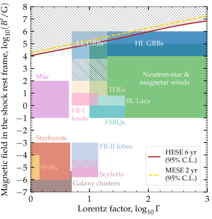
Figure 1: Upper limit on the average magnetic field ($B^{\prime}$) as a function of the bulk Lorentz factor ($\Gamma$) of the astrophysical sources of TeV–PeV neutrinos, derived from 6 years of IceCube High Energy Starting Events Kopper et al. (2016); IceCube Collaboration (2015); Kopper (2018) (HESE) and 2 years of Medium Energy Starting Events Aartsen et al. (2015b); IceCube Collaboration (2017) (MESE). We include approximate ranges for candidate sources: neutron-star and magnetar winds Arons (2003); Bucciantini et al. (2008); Mereghetti (2008); Ptitsyna and Troitsky (2010), low- Ghisellini et al. (2007); Toma et al. (2007) and high-luminosity Piran (2005); Ghirlanda et al. (2018) gamma-ray bursts (LL GRBs, HL GRBs), blazars Ghisellini et al. (2017) [flat spectrum radio quasars (FSRQs), BL Lacs], tidal disruption events Burrows et al. (2011) (TDEs), starbursts Thompson et al. (2006a); Ackermann et al. (2012), supernovae Murase et al. (2019) (SNe), supernova remnants Wang et al. (2007) (SNRs), galaxy clusters Brunetti and Jones (2014); Voit (2005), and active galactic nuclei (Seyfert Ptitsyna and Troitsky (2010); Paliya et al. (2019), FR-I Becker Tjus et al. (2014), FR-II galaxies Becker Tjus et al. (2014)). The average magnetic field strength is limited to be smaller than $10$ kG–$10$ MG.

We use TeV–PeV astrophysical neutrinos as “cosmic magnetometers” that constrain the average magnetic field of the neutrino sources. Because candidate source classes span a wide range of magnetic field strengths, this constraint narrows down the identity of the sources.

We look for imprints left by the magnetic field of the sources on the diffuse neutrino flux. On the one hand, the average magnetic field must be strong enough to accelerate protons up to PeV energies. On the other hand, it cannot be too strong, or else proton energy losses via synchrotron radiation would lower the maximum proton energy and preclude the production of high-energy neutrinos. Further, intermediate magnetic field strengths may induce synchrotron losses in secondary pions and muons that decay into neutrinos, affecting their energy spectrum and flavor composition. We look for evidence of the interplay of these effects in public IceCube data.

Figure 1 shows that our results limit the average magnetic field to be weaker than $10$ kG–$10$ MG. This partially disfavors low-luminosity GRBs as the main sites of TeV–PeV neutrino production. Our work builds on and extends the constraints on magnetic fields of a few MG found by Ref. Winter (2013) using the first 2 years of IceCube data, by using 4 more years of IceCube data, two different IceCube event samples, a significantly refined computation of event spectra, and a Bayesian statistical treatment.

II Energy losses via synchrotron radiation

We consider a generic scenario that captures the key features common to high-energy neutrino source candidates. Neutrinos are produced in an outflow of baryon-loaded material with a bulk Lorentz factor $\Gamma$ and magnetic field strength $B^{\prime}$. To keep our scenario generic, we consider protons only; see, e.g., Refs. Boncioli et al. (2017); Biehl et al. (2018a) for production scenarios including heavier nuclei and nuclear cascades. Here and below, primed quantities are expressed in the rest frame of the neutrino production region, i.e., the shock rest frame; all other quantities are in the comoving frame of the production region or, after accounting for redshift effects, in the frame of the observer.

Sources accelerate protons via collisionless shocks in the magnetized outflow, up to a maximum energy $E_{p}^{\prime\max}$ Hillas (1984). To treat all candidate sources on an equal footing, we assume that $E_{p}^{\prime\max}$ is limited by proton synchrotron losses. However, alternative energy-loss mechanisms may be dominant in some source classes Murase and Ioka (2013); Tamborra and Ando (2015); Fang (2015) or the flavor content may be affected in an energy-dependent fashion by oscillations in dense media Carpio and Murase (2020); Razzaque et al. (2004); Ando and Beacom (2005); we comment on source-specific features later. Protons reach their maximum energy when two time scales become comparable: their acceleration time scale, $t_{\rm acc}^{\prime}=E_{p}^{\prime}/(\eta eB^{\prime})$, where $e$ is the electron charge and $\eta$ is the acceleration efficiency, and their synchrotron energy-loss time scale, $t_{\rm sync}^{\prime}=9m_{p}^{4}/(4e^{4}B^{\prime 2}E_{p}^{\prime})$, where $m_{p}$ is the proton mass. In the comoving frame, this yields $E_{p}^{\max}\approx 2\times 10^{11}\leavevmode\nobreak\ \Gamma(\eta/B^{\prime})^{1/2}$ GeV. Since sources must be rather efficient accelerators, we fix $\eta=1$ from here on, and comment later on how the neutrino emission changes with $\eta$.

The interactions of protons with matter and radiation produce secondary pions and muons that, upon decaying, generate neutrinos Stecker (1979): $\pi^{+}\to\mu^{+}+\nu_{\mu}$, followed by $\mu^{+}\to e^{+}+\nu_{e}+\bar{\nu}_{\mu}$, and the charge-conjugated processes Kelner et al. (2006); Kelner and Aharonian (2008). On average, a pion receives 1/5 of the proton energy, each neutrino from muon decay receives 1/3 of the muon energy, and each final-state neutrino receives 1/4 of the pion energy. Following theory expectations, each source emits neutrinos distributed in energy as $E_{\nu}^{\prime 2}\leavevmode\nobreak\ dN_{\nu}/dE_{\nu}^{\prime}\propto E_{\nu}^{\prime 2-\alpha_{\nu}}e^{-E_{\nu}^{\prime}/E_{\nu}^{\prime\max}}$, where $E_{\nu}^{\prime}$ is the neutrino energy. We assume that the maximum neutrino energy, $E_{\nu}^{\prime\max}$, and the spectral index, $\alpha_{\nu}$, are common to neutrinos and anti-neutrinos of all flavors. Because each neutrino receives 1/20 of the parent proton energy, $E_{\nu}^{\max}=E_{p}^{\max}/20$ and is affected by synchrotron losses. Below, we show how synchrotron losses of the secondaries affect $\alpha_{\nu}$.

For the secondary pions, synchrotron losses are significant if they occur within a time scale shorter than the pion decay time, $t_{\rm dec}^{\prime}=\tau_{\pi}E_{\pi}^{\prime}/m_{\pi}$, where $E_{\pi}^{\prime}$, $\tau_{\pi}$, and $m_{\pi}$ are the pion energy, lifetime, and mass. In the comoving frame, this occurs at neutrino energies above $E_{\nu,\pi}^{\rm sync}\approx 3\times 10^{10}(\Gamma/B^{\prime})$ GeV. By analogous arguments, for the secondary muons, synchrotron losses are significant at energies above $E_{\nu,\mu}^{\rm sync}\approx 2\times 10^{9}(\Gamma/B^{\prime})$ GeV.

Below $E_{\nu,\pi}^{\rm sync}$, $\alpha_{\nu}$ is solely determined by the parent proton and photon spectra. In lieu of detailed modeling, we parametrize it as $\alpha_{\nu}(E_{\nu}<E_{\nu,\pi}^{\rm sync})=\gamma$, where $\gamma\in[2,3]$ is a free parameter whose value we vary later. At $E_{\nu,\mu}^{\rm sync}$, the neutrino spectrum coming from the decay of muons steepens by $\sim$$E_{\nu}^{-2}$, so these neutrinos become sub-dominant and the flux is mainly from neutrinos produced in the direct decay of pions. As a result, the flavor composition of the emitted neutrinos, i.e., the fraction $f_{\alpha,{\rm S}}$ ($\alpha=e,\mu,\tau$) of neutrinos plus anti-neutrinos of each flavor, changes from that of the full pion decay chain, $\left(f_{e,{\rm S}},f_{\mu,{\rm S}},f_{\tau,{\rm S}}\right)=\left(1/3,2/3,0\right)$, at $E_{\nu}<E_{\nu,\mu}^{\rm sync}$, to that coming from the direct pion decay only, $\left(0,1,0\right)$, at $E_{\nu}\geq E_{\nu,\mu}^{\rm sync}$. At even higher energies $E_{\nu}\geq E_{\nu,\pi}^{\rm sync}$, the neutrino spectrum from pion decays itself steepens by $\sim$$E_{\nu}^{-2}$, so $\alpha_{\nu}(E_{\nu}\geq E_{\nu,\pi}^{\rm sync})=\gamma+2$.

III Diffuse flux of high-energy neutrinos

The luminosity of $\nu_{\alpha}+\bar{\nu}_{\alpha}$ that reaches Earth from a single source located at redshift $z$, in the frame of the observer, is

$$J_{\nu_{\alpha}} (E_{\nu},z,\gamma,\Gamma,B^{\prime})\propto f_{\alpha,\oplus}(E_{\nu}(1+z),\Gamma,B^{\prime})$$

$$\times\leavevmode\nobreak\ [E_{\nu}(1+z)]^{2-\alpha_{\nu}(E_{\nu},\gamma,\Gamma,B^{\prime})}\leavevmode\nobreak\ e^{-E_{\nu}(1+z)/E_{\nu}^{\max}(\Gamma,B^{\prime})}\;.$$

Because flavors mix, neutrino flavor conversions en route to Earth change the flavor composition into $f_{\alpha,\oplus}=\sum_{\beta=e,\mu,\tau}P_{\beta\alpha}f_{\beta,{\rm S}}$, where $P_{\beta\alpha}$ is the average $\nu_{\beta}\to\nu_{\alpha}$ conversion probability Pakvasa (2008). To compute it, we fix the mixing parameters to their best-fit values from the recent NuFit 4.1 global fit to neutrino oscillation data Esteban et al. (2019); NuFit , assuming normal neutrino mass ordering. The flavor composition changes from $(f_{e,\oplus},f_{\mu,\oplus},f_{\tau,\oplus})\approx(1/3,1/3,1/3)$ at $E_{\nu}<E_{\nu,\mu}^{\rm sync}$ to roughly $(1/5,2/5,2/5)$ at $E_{\nu}\geq E_{\nu,\mu}^{\rm sync}$.

To compute the diffuse flux of $\nu_{\alpha}+\bar{\nu}_{\alpha}$, $\Phi_{\nu_{\alpha}}$, we integrate the contribution from all sources up to redshift $z_{\max}=4$; sources at higher redshifts contribute negligibly. To describe a variety of candidate source classes, we adopt the following parametrization for the source density: $\rho\propto(1+z)^{m}$ up to $z_{c}\equiv 1.5$, and $\rho\propto(1+z_{c})^{m}$ at $z>z_{c}$. Later, we let the value of $m$ float. Thus, the diffuse energy flux is

$$E_{\nu}^{2}\Phi_{\nu_{\alpha}}(E_{\nu},\gamma,m,\Gamma,B^{\prime})$$ (2)

$$\qquad\propto\int_{0}^{z_{\max}}dz\frac{\rho(z,m)}{h(z)(1+z)^{2}}J_{\nu_{\alpha}}(E_{\nu},z,\gamma,\Gamma,B^{\prime})\;,$$

where $h(z)\equiv[\Omega_{\Lambda}+(1+z)^{3}\Omega_{m}]^{1/2}$ is the adimensional Hubble parameter, and $\Omega_{\Lambda}=0.685$ and $\Omega_{m}=0.315$ are the energy densities of vacuum and matter Aghanim et al. (2018); Tanabashi et al. (2018).

We assume that all of the contributing sources have the same values of $\gamma$, $\Gamma$, and $B^{\prime}$. In reality, these parameters likely follow distributions that are presently unknown. By assuming values that are common to all sources, we aim to constrain their population-averaged values.

In summary, if the average $B^{\prime}$ is large, the synchrotron losses of protons and secondaries may visibly affect the spectral index $\alpha_{\nu}$, flavor composition $f_{\alpha,\oplus}$, and maximum energy $E_{\nu}^{\max}$ of the diffuse neutrino flux Kashti and Waxman (2005); Kachelriess et al. (2008); Lipari et al. (2007); Baerwald et al. (2011); Winter (2012). These features are softened and spread out in energy by the redshift distribution of the sources.

Figure 2 shows sample fluxes for two choices of $B^{\prime}$. The change to the flavor composition due to muon synchrotron cooling is prominent in both fluxes, at $E_{\nu}\approx 2$ PeV and 200 TeV for $B^{\prime}=30$ kG and 300 kG, respectively. For the flux with $B^{\prime}=300$ kG, the spectral softening due to pion synchrotron cooling is also visible around 3 PeV. In Fig. 2, the flux dampening due to proton synchrotron cooling occurs at energies higher than shown. This is true for viable neutrino source candidates, which must be efficient accelerators: as long as $\eta\gtrsim 0.01$, proton cooling becomes important only after muon cooling does, provided $B^{\prime}$ is at least a few G.

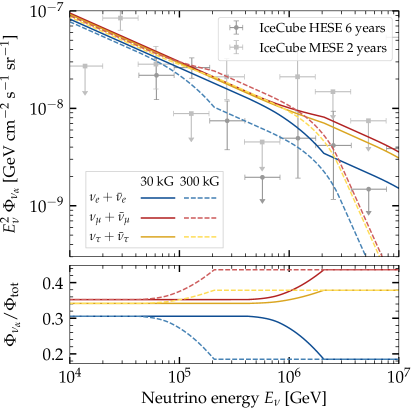
Figure 2: Top: Sample diffuse astrophysical neutrino fluxes at Earth, as a function of the neutrino energy, for two illustrative values of the magnetic field strength of the sources, $B^{\prime}$. In this plot only, the flux parameters are fixed to illustrative values: $\gamma=2.50$, $\Gamma\approx 32$, $m=1.5$, and the normalization of each flux, at $E_{\nu}=100$ TeV, to $3\times 10^{-8}$ GeV cm^-1 s^-1 sr^-1. Data points show the spectra of the IceCube HESE Kopper et al. (2016); IceCube Collaboration (2015); Kopper (2018) and MESE Aartsen et al. (2015b); IceCube Collaboration (2017) event samples. Bottom: Flavor composition $\Phi_{\nu_{\alpha}}/\Phi_{\rm tot}$ ($\alpha=e,\mu,\tau$) of the diffuse flux, where $\Phi_{\rm tot}\equiv\sum_{\alpha}\Phi_{\nu_{\alpha}}$. The spectral breaks and changes to the flavor composition are due to the synchrotron cooling of muons and pions.

III.1 Neutrino propagation through the Earth

Upon reaching Earth, high-energy neutrinos propagate from its surface, through its interior, and up to the South Pole, where IceCube is located. Neutrino-nucleon interactions along the way modify the neutrino flux. At these energies, neutrinos deep-inelastic scatter off of nucleons. Charged-current (CC) interactions ($\nu_{\alpha}+N\to\alpha+X$, where $X$ are final-state hadrons) remove neutrinos from the flux. Neutral-current (NC) interactions ($\nu_{\alpha}+N\to\nu_{\alpha}+X$) redistribute neutrinos from high to low energies.

To compute the neutrino flux that reaches IceCube, we adopt the Preliminary Reference Earth Model Dziewonski and Anderson (1981) for the matter density inside the Earth and assume that matter is isoscalar, i.e., made up of equal numbers of protons and neutrons. At these energies, there are no matter-driven flavor transitions Wolfenstein (1978); Mikheyev and Smirnov (1985). The flux at IceCube is different for different propagation directions, flavors, and for neutrinos and anti-neutrinos. We use nuSQuIDS Argüelles et al. (2015, 2018a, 2019a) to compute the fluxes of $\nu_{\alpha}$ and $\bar{\nu}_{\alpha}$, astrophysical and atmospheric (see below), that reach IceCube.

III.2 Atmospheric backgrounds

The main backgrounds to our analysis are high-energy atmospheric neutrinos and muons produced in the interaction of cosmic rays in the atmosphere of the Earth. They are especially important below 100 TeV Beacom and Candia (2004). In IceCube, the contamination of atmospheric neutrinos is mitigated by using part of the detector as a self-veto Schönert et al. (2009); Gaisser et al. (2014); Aartsen et al. (2015b); Argüelles et al. (2018b), and the contamination of atmospheric muons, by using a surface array of water-Cherenkov tanks as veto Aartsen et al. (2013b); Tosi and Pandya (2020). In our analysis, we account for these backgrounds and vetoes.

For atmospheric neutrinos, we use the same state-of-the-art tools used by the IceCube Collaboration: MCEq Fedynitch et al. (2015); Fedynitch (2019) to generate neutrino fluxes produced in the decay of pions and kaons, and nuVeto Argüelles et al. (2018b, 2019b) to compute the flux reduction due to the self-veto for HESE events. For MESE events, the self-veto is already included in the effective detector area; see Appendix A.2. We do not consider prompt atmospheric neutrinos produced in the decay of charmed mesons, since they have not been observed and are subject to stringent upper limits Aartsen et al. (2015c).

For atmospheric muons, we approximate the flux that reaches IceCube, after the surface veto, following the procedure in Ref. Palomares-Ruiz et al. (2015) for HESE events, and extending it for MESE events, as detailed in Appendix A.3.

III.3 High-energy neutrino detection

In IceCube, neutrinos are detected when they scatter off of nucleons in the Antarctic ice and trigger particle showers that emit Cherenkov light that is collected by photomultipliers buried 1.5–2.5 km underground. From the amount of light collected and from its spatial and temporal profiles, IceCube infers the energy deposited, $E_{\rm dep}$, and the neutrino arrival direction, $\cos\theta_{z}$, where $\theta_{z}$ is the zenith angle measured from the South Pole.

We focus on “starting” events, where the neutrino interaction occurs inside the instrumented volume, so that $E_{\rm dep}$ is close to the energy of the interacting neutrino. In the TeV–PeV range, events are predominantly “showers,” roughly spherical light profiles triggered mainly by $\nu_{e}$ and $\nu_{\tau}$, and “tracks,” elongated light profiles made by final-state muons, triggered mainly by $\nu_{\mu}$.

For an incoming flux of astrophysical or atmospheric neutrinos along a given direction, we forecast the spectra $dN/dE_{\rm dep}$ of showers and tracks following Ref. Palomares-Ruiz et al. (2015); see Appendix A.1. We account for differences in deposited energy for different flavors, CC vs. NC, and decay channels of final-state particles, and for the $\sim$$13\%$ detector energy resolution.

IV Statistical analysis

We compare forecasted event spectra computed with different values of the flux parameters against two public IceCube event samples: 6 years of High Energy Starting Events (HESE) Kopper et al. (2016); IceCube Collaboration (2015); Kopper (2018) and 2 years of Medium Energy Starting Events (MESE) Aartsen et al. (2015b); IceCube Collaboration (2017). The HESE sample has 58 showers and 22 tracks with $E_{\rm dep}=$ 18 TeV–2 PeV. The MESE sample has 278 showers and 105 tracks with $E_{\rm dep}=$ 330 GeV–1.3 PeV. The samples provide $E_{\rm dep}$ and $\cos\theta_{z}$ for each event. A few events are common to both samples, but since they cannot be singled out, we treat the samples separately to avoid double-counting.

In the HESE sample, below a few tens of TeV, roughly half of the events are of atmospheric origin and half of astrophysical origin; above, they are mostly of astrophysical origin Kopper (2018). The MESE sample extends to lower energies, where the atmospheric contamination is higher. We restrict MESE events to $E_{\rm dep}\geq 20$ TeV in order to avoid a dominant atmospheric contamination that, according to our tests, would otherwise skew our results. This is the same energy region of validity of the astrophysical neutrino component in the IceCube MESE analysis Aartsen et al. (2015b).

We adopt a Bayesian approach to search for evidence of synchrotron cooling and constrain $B^{\prime}$. For a sample of $N_{\rm obs}$ IceCube events, our likelihood function is

$$\mathcal{L}(\gamma,m,\Gamma,B^{\prime},N_{\rm ast},N_{\rm atm},N_{\mu})$$ (3)

$$=e^{-N_{\rm ast}-N_{\rm atm}-N_{\mu}}\prod_{i=1}^{N_{\rm obs}}\mathcal{L}_{i}(\gamma,m,\Gamma,B^{\prime},N_{\rm ast},N_{\rm atm},N_{\mu})\;,$$

where $N_{\rm ast}$, $N_{\rm atm}$, and $N_{\mu}$ are, respectively, the number of events due to astrophysical neutrinos, atmospheric neutrinos, and atmospheric muons. The partial likelihood for the $i$-th event compares the odds of it being due to the different fluxes: $\mathcal{L}_{i}=N_{\rm ast}\mathcal{P}_{i,{\rm ast}}(\gamma,m,\Gamma,B^{\prime})+N_{\rm atm}\mathcal{P}_{i,{\rm atm}}+N_{\mu}\mathcal{P}_{i,\mu}$, where $\mathcal{P}_{i,{\rm ast}}$, $\mathcal{P}_{i,{\rm atm}}$, and $\mathcal{P}_{i,\mu}$ are the probability distribution functions for this event to have been generated by astrophysical neutrinos, atmospheric neutrinos, and atmospheric muons. For astrophysical neutrinos, $\mathcal{P}_{i,{\rm ast}}=(dN_{i}/dE_{\rm dep})/\int dE_{\rm dep}(dN_{i}/dE_{\rm dep})$, where the event spectrum is computed using the flux along the direction of the $i$-th event, and similarly for atmospheric neutrinos. The procedure differs slightly for HESE and MESE, and for muons; see Appendix A.

We maximize the likelihood separately for the HESE and MESE samples. For $N_{\rm ast}$, $N_{\rm atm}$, $N_{\mu}$, and $\gamma$ (only for HESE), we adopt informed priors based on the HESE Kopper (2018) and MESE Aartsen et al. (2015b) analyses by IceCube. For $m$, $\log_{10}\Gamma$, and $\log_{10}(B^{\prime}/{\rm G})$, we adopt wide uniform priors to avoid introducing bias. See Appendix B.1 for details about the priors. To maximize the likelihood, we use the efficient Bayesian sampler MultiNest Feroz and Hobson (2008); Feroz et al. (2009, 2013); Buchner et al. (2014). We quantify the preference for synchrotron-loss features via the Bayes factor, $K\equiv Z_{\rm signal}/Z_{\rm null}$, that compares the evidence, or marginalized likelihood, in favor of their presence, $Z_{\rm signal}$, over their absence, $Z_{\rm null}$. Appendix B contains details of the statistical analysis.

Table 1: Allowed marginalized ranges of the average Lorentz factor, $\Gamma$, and magnetic field strength, $B^{\prime}$, of the sources of high-energy astrophysical neutrinos, obtained using the public IceCube 6-year HESE Kopper et al. (2016); IceCube Collaboration (2015); Kopper (2018) and 2-year MESE Aartsen et al. (2015b); IceCube Collaboration (2017) event samples. The preference for synchrotron-loss features in the data is insignificant; see the main text.

Parameter	HESE		MESE ($E_{\rm dep}>20$ TeV)
	Mean $\pm 1\sigma$	95% C.L.	Mean $\pm 1\sigma$	95% C.L.
$\log_{10}\Gamma$	$1.78\pm 0.86$	$[0.22,2.86]$	$1.16\pm 0.90$	$[0.85,6.75]$
$\log_{10}(B^{\prime}/{\rm G})$	$2.96\pm 1.78$	$[0.23,5.97]$	$4.82\pm 1.20$	$[0.10,2.82]$

V Results

Table 1 shows the allowed ranges of $\Gamma$ and $B^{\prime}$ that result from our analysis. Both event samples prefer values of $B^{\prime}$ that push the synchrotron-loss features to energies beyond a few PeV, past the energies covered by the samples. For both samples, $\log_{10}K\approx 0.3$, i.e., the evidence for synchrotron-loss features in the data is insignificant Jeffreys (1939). Hence, we place upper limits on $B^{\prime}$.

Figure 1 shows our limits on $B^{\prime}$ as a function of $\Gamma$, after marginalizing over all other likelihood parameters. The limits are isocontours of $E_{\nu,\mu}^{\rm synch}$ and $E_{\nu,\pi}^{\rm synch}$ and, in agreement with Ref. Winter (2013), we find that they are predominantly driven by the absence of a spectral break, rather than by the absence of a change in flavor composition, to which there is currently little sensitivity. The limits are similar for both samples because, after selecting MESE events with $E_{\rm dep}\geq 20$ TeV, both samples cover roughly the same $E_{\rm dep}$ range. The MESE limit is worse because there are 26 fewer MESE than HESE events.

Our results disfavor a predominant origin of the TeV–PeV neutrinos in astrophysical sources with average magnetic field stronger than $\sim$$10(1+\Gamma)$ kG, i.e., $10$ kG–$10$ MG approximately. This partially includes low-luminosity GRBs Gupta and Zhang (2007); Murase et al. (2006); Kashiyama et al. (2013); Murase and Ioka (2013); Tamborra and Ando (2015); Senno et al. (2016); Zhang et al. (2018). Fast radio bursts (FRBs) have been considered as potential neutrino sources, but their feasibility as such depends on their origin, which is currently subject of intense investigation. So far, direct searches have found no evidence for FRBs as high-energy neutrino sources Fahey et al. (2017); Aartsen et al. (2018b); Albert et al. (2019); Aartsen et al. (2019b); Metzger et al. (2020). If FRBs are connected to magnetars Li et al. (2014); Dey et al. (2016); Andersen et al. (2020); Ridnaia et al. (2020); Bochenek et al. (2020); Tavani et al. (2020), then our limits would disfavor relativistic outflows in FRBs as regions of copious production of high-energy neutrinos. Our results also disfavor the non-thermal emission of high-energy neutrinos from the crusts of magnetars and neutron stars Zhang et al. (2003), with $B^{\prime}\approx 10^{14}$–$10^{15}$ G, but these sites are not expected to be efficient hadronic accelerators.

Sources with an intermediate field of $10$ kG–$1$ MG—high-luminosity GRBs Waxman and Bahcall (1997); Murase and Nagataki (2006); Hümmer et al. (2012); Zhang and Kumar (2013); Liu and Wang (2013); Baerwald et al. (2015); Tamborra and Ando (2015, 2016); Biehl et al. (2018a), blazars Stecker et al. (1991); Atoyan and Dermer (2001); Murase et al. (2012a); Padovani and Resconi (2014); Kimura et al. (2015); Padovani et al. (2015); Cerruti et al. (2019); Liu et al. (2019); Palladino et al. (2019); Keivani et al. (2018); Murase et al. (2018); Gao et al. (2019); Rodrigues et al. (2019); Petropoulou et al. (2020), pulsar and magnetar winds Arons (2003); Ptitsyna and Troitsky (2010); Fang (2015); Fang and Metzger (2017); Fang et al. (2016)—remain viable candidates according to our analysis. These are electromagnetically luminous and relatively abundant sources; at face value, they are ideal neutrino emitters. However, they are strongly constrained by dedicated searches: the contribution of high-luminosity GRBs and blazars is restricted to be less than 2% Aartsen et al. (2017b) and 15% Smith et al. (2020); Aartsen et al. (2017a) of the diffuse flux, respectively.

Sources with a weak field—non-blazar AGN Anchordoqui et al. (2004); Stecker (2005); Álvarez-Muñiz and Mészáros (2004); Stecker (2013); Becker Tjus et al. (2014); Hooper et al. (2019); Smith et al. (2020), TDEs Dai and Fang (2017); Lunardini and Winter (2017); Biehl et al. (2018b); Winter and Lunardini (2020); Murase et al. (2020), starburst galaxies Loeb and Waxman (2006); Stecker (2007); Thompson et al. (2006b); He et al. (2013); Tamborra et al. (2014); Chang and Wang (2014); Hooper et al. (2019); Peretti et al. (2020), supernovae Horiuchi and Ando (2008); Murase (2018); Petropoulou et al. (2017); Senno et al. (2018); Murase et al. (2019); Esmaili and Murase (2018); Fang et al. (2020a), supernova remnants Wang et al. (2007); Villante and Vissani (2008); Liu et al. (2014); Chakraborty and Izaguirre (2015), and galaxy clusters Dar and Shaviv (1996); Berezinsky et al. (1997); De Marco et al. (2006); Kotera et al. (2009); Zandanel et al. (2015); Senno et al. (2015)—remain viable candidates in a broader sense and may account for a large fraction of the diffuse neutrino flux. The neutrino emission from these sources is largely unconstrained by direct searches due to their high abundance and low luminosity per source Silvestri and Barwick (2010); Murase and Waxman (2016); Mertsch et al. (2017); Capel et al. (2020); Fang et al. (2020b).

While we have derived our results assuming that the sources emit neutrinos with a power-law energy distribution, they are valid within a more general framework. We have repeated our analysis using a broken power-law energy distribution where the spectral index $\alpha_{\nu}$ steepens by $\Delta\alpha_{\nu}$ after a break energy $E_{\nu,{\rm br}}^{\prime}$. This steepening mimics a production scenario where neutrinos inherit the peaked shape of a parent photon spectrum or the pile-up of low-energy neutrinos produced by the decay of synchrotron-cooled muons; see, e.g., Refs. Waxman and Bahcall (1999); Mannheim et al. (2001); Mücke et al. (2000); Kelner and Aharonian (2008); Hümmer et al. (2010). Also in this case, we find no evidence of synchrotron-loss features in the HESE and MESE samples. The resulting upper limits on $B^{\prime}$ are very similar to those shown in Fig. 1.

VI Summary and outlook

The magnetic field of the sources that populate the high-energy Universe remain enigmatic. At the same time, one of the main goals of neutrino astronomy is to identify the sources of the TeV–PeV neutrinos seen by IceCube. We have introduced a new way to address these two long-standing questions, by using high-energy neutrinos as cosmic magnetometers.

We look in the diffuse flux of TeV–PeV astrophysical neutrinos for imprints left by the magnetic field of their sources on the energy spectrum and flavor composition. These imprints originate in the energy losses via synchrotron radiation of the protons, pions, and muons that produce the neutrinos. We find no evidence in 6 years of IceCube high-energy events (HESE) and 2 years of medium-energy events (MESE). Thus, we constrain the average magnetic field strength of the neutrino sources to be smaller than $10$ kG–$10$ MG. Consequently, we partially disfavor low-luminosity GRBs as the predominant sources of TeV–PeV neutrinos, but sources with a weak magnetic field—AGN, TDEs, SNe, SNRs, starburst galaxies, magnetar and neutron star winds, and galaxy clusters—remain viable candidates.

Because we use a generic model of neutrino production, our results apply to a wide range of candidate source classes. Future work may explore source- and population-dependent modeling in order to boost the sensitivity to specific source classes. Further refinements include a detailed treatment of the source physics and cosmic-ray acceleration, the interaction not only of protons, but also of nuclei, additional neutrino-production channels, and non-synchrotron losses; see, e.g., Refs. Anchordoqui et al. (2008); Hümmer et al. (2010); Petropoulou (2014); Boncioli et al. (2017); Morejón et al. (2019); Fang (2015). Further, the acceleration of secondary muons, pions, and kaons, which we have neglected, could play an important role in mitigating synchrotron cooling in astrophysical environments with efficient particle diffusion Murase et al. (2012b); Winter et al. (2014).

In the future, larger detectors, like the planned IceCube-Gen2 Aartsen et al. (2020), will be able to detect neutrinos at a higher rate, at energies beyond the PeV scale, and will have improved sensitivity to changes in flavor composition with energy Bustamante et al. (2015). This will allow to place tighter bounds on the source magnetic field and probe the existence of synchrotron-loss features at higher energies, i.e., of magnetic fields weaker than the ones that we are currently sensitive to.

Appendix A Overview of the calculation of event spectra at IceCube

A.1 HESE events

To compute the differential spectrum $dN/dE_{\rm dep}$ of HESE events at IceCube, we follow the detailed procedure from Ref. Palomares-Ruiz et al. (2015). The spectra of showers and tracks are computed separately, accounting in each case for the contributing interactions of all flavors of neutrinos and anti-neutrinos. The event rates are computed from first principles, i.e., from the effective IceCube mass and the deep-inelastic-scattering neutrino-nucleon differential cross section for $\nu_{\alpha}$ and $\bar{\nu}_{\alpha}$, based on the CTEQ14 parton distribution functions Dulat et al. (2016). The procedure accounts for differences in deposited energy for different flavors, CC vs. NC, and decay channels of final-state particles, and for the $\sim$$13\%$ detector energy resolution. We defer to Ref. Palomares-Ruiz et al. (2015) for the explanation of the full procedure and to Appendix A in Ref. Bustamante et al. (2020) and Appendix C in Ref. Bustamante (2020) for an overview.

A.2 MESE events

To compute the spectrum of MESE events, we use the IceCube effective area, $A_{{\rm eff}}^{s,t}(E_{\nu},E_{\rm rec},\cos\theta_{z},\cos\theta_{z,{\rm rec}})$, provided by the IceCube Collaboration for its 2-year MESE analysis Aartsen et al. (2015b); IceCube Collaboration (2017), as a function of true neutrino energy $E_{\nu}$, reconstructed (i.e., deposited) energy $E_{\rm rec}$, true neutrino direction $\cos\theta_{z}$, and reconstructed direction $\cos\theta_{z,{\rm rec}}$. The effective area is provided separately for each neutrino species $s=\nu_{e},\bar{\nu}_{e},\nu_{\mu},\bar{\nu}_{\mu},\nu_{\tau},\bar{\nu}_{\tau}$, and topology $t=$ sh (shower), tr (track). It includes the effects of the MESE self-veto and of the mapping between true and reconstructed quantities.

In general, given diffuse neutrino fluxes $\Phi_{s}$, the number of detected events at IceCube after a time $T$, at a given reconstructed energy and direction is

$$N_{t}(E_{\rm rec},\cos\theta_{z,{\rm rec}})=2\pi T\sum_{s}\int dE_{\nu}\int_{-1}^{+1}d\cos\theta_{z}A_{{\rm eff}}^{s,t}(E_{\nu},E_{\rm rec},\cos\theta_{z},\cos\theta_{z,{\rm rec}})\Phi_{s}(E_{\nu},\cos\theta_{z})\;.$$ (4)

The sum over $s$ adds the contribution of all flavors of neutrinos and anti-neutrinos that make showers or tracks.

For our analysis, we make two modifications to this expression. First, because the effective area is binned in all of its input parameters, we change the integrals in Eq. (4) for sums over bins. To do this, we write the effective area in the $j$-th bin of $E_{\rm rec}$, the $k$-th bin of $\cos\theta_{z,{\rm rec}}$, the $l$-th bin of $E_{\nu}$, and the $m$-th bin of $\cos\theta_{z}$ as $A_{{\rm eff},jklm}^{s,t}$. Second, because there are only two bins of $\cos\theta_{z,{\rm rec}}$ provided ([0.2,1.0] for downgoing events and [-1,0.2] for upgoing events) we assume that $\cos\theta_{z,{\rm rec}}\approx\cos\theta_{z}$, i.e., that the reconstructed direction closely follows the neutrino direction. This means that, in our computation, $m=k$ always. Thus, if the requested values of $E_{\rm rec}$ and $\cos\theta_{z,{\rm rec}}$ on the left-hand side of Eq. (4) are contained, respectively, inside their $j^{\ast}$-th and $k^{\ast}$-th bins, then Eq. (4) simplifies to

$$N_{t}(E_{\rm rec},\cos\theta_{z,{\rm rec}})=2\pi T\sum_{s}\sum_{l=1}^{N_{E_{\nu}}}A_{{\rm eff},j^{\ast}k^{\ast}lk^{\ast}}^{s,t}\int_{E_{\nu,l}^{\min}}^{E_{\nu,l}^{\max}}dE_{\nu}\Phi_{s}(E_{\nu},\cos\theta_{z,{\rm rec}})\;,$$ (5)

where $N_{E_{\nu}}$ is the number of bins of $E_{\nu}$, and $E_{\nu,l}^{\min}$ and $E_{\nu,l}^{\max}$ are the minimum and maximum energies in the $l$-th bin of $E_{\nu}$.

After this, the statistical procedure described in the main text proceeds similarly for MESE and HESE events. There are only two differences. The first one is in the computation of the spectra of atmospheric muons, which we describe in Appendix A.3. The second one is in the computation of the astrophysical and atmospheric probability distribution functions, $\mathcal{P}_{i,{\rm ast}}$ and $\mathcal{P}_{i,{\rm atm}}$, for the $i$-th MESE event. The probability distribution functions are computed similarly as for HESE events, but using the total event rate, Eq. (5), instead of the differential event rate (see the main text). For astrophysical neutrinos, this is

$$\mathcal{P}_{i,{\rm ast}}=\frac{N_{t}(E_{{\rm rec},i},\cos\theta_{z,{\rm rec},i})}{\sum_{j=1}^{N_{E_{\rm rec}}}N_{t}(E_{{\rm rec},j},\cos\theta_{z,{\rm rec},i})}\;,$$ (6)

where $t$ depends on whether this event is a shower or track, $N_{t}$ is computed using the astrophysical neutrino fluxes, $E_{{\rm rec},i}$ and $\cos\theta_{z,{\rm rec},i}$ are the deposited energy and direction of the $i$-th event, and $N_{E_{\rm rec}}$ is the number of bins of $E_{\rm rec}$. The calculation is analogous for $\mathcal{P}_{i,{\rm atm}}$, changing only the astrophysical fluxes for the atmospheric fluxes in Eq. (5).

A.3 Atmospheric muon background in the HESE and MESE samples

To compute the spectra of atmospheric muons that reaches IceCube, we follow the procedure from Ref. Palomares-Ruiz et al. (2015), which was designed for HESE events. We extend its application also to MESE events.

Instead of simulating the propagation of muons through the Earth and applying a surface veto ourselves to mitigate their contamination, the procedure in Ref. Palomares-Ruiz et al. (2015) directly computes the distribution $dN_{\mu}/dE_{\rm dep}\propto E_{\rm dep}^{-\gamma_{\mu}}$ of muons that pass the veto. The value of the spectral index $\gamma_{\mu}$ varies for HESE versus MESE events. To compute it, we compare the number of passing muons below and above a certain deposited energy $E_{\rm dep}^{\ast}$, respectively,

$$N_{\mu}(<E_{\rm dep}^{\ast}) = \frac{1}{1-\gamma_{\mu}}\left[(E_{\rm dep}^{\ast})^{1-\gamma_{\mu}}-(E_{\rm dep}^{\rm min})^{1-\gamma_{\mu}}\right]\;,$$ (7)

$$N_{\mu}(\geq E_{\rm dep}^{\ast}) = \frac{-1}{1-\gamma_{\mu}}(E_{\rm dep}^{\ast})^{1-\gamma_{\mu}}\;,$$ (8)

where $E_{\rm dep}^{\rm min}$ is the minimum deposited energy in the event sample. With this, the spectral index is

$$\gamma_{\mu}=1-\ln\left(1+\frac{N_{\mu}(<E_{\rm dep}^{\ast})}{N_{\mu}(\geq E_{\rm dep}^{\ast})}-\frac{E_{\rm dep}^{\rm min}}{E_{\rm dep}^{\ast}}\right)\;.$$ (9)

For HESE events, we compute $\gamma_{\mu}$ using the muon rates reported in the 3-year IceCube HESE analysis Aartsen et al. (2014). Table IV in Ref. Aartsen et al. (2014) reports 8 passing muons below $E_{\rm dep}^{\ast}=60$ TeV and 0.4 passing muons above it. In that sample, $E_{\rm dep}^{\rm min}=28$ TeV. Therefore, for HESE events, $\gamma_{\mu}\approx 5$, as reported by Ref. Palomares-Ruiz et al. (2015).

For MESE events, we compute $\gamma_{\mu}$ using the muon rates reports in the 2-year IceCube MESE analysis Aartsen et al. (2015b). Figure 8 in Ref. Aartsen et al. (2015b) reports 64.78 passing muons below $E_{\rm dep}^{\ast}=50$ TeV and 0.44 passing muons above it. In that sample, $E_{\rm dep}^{\rm min}=0.33$ TeV. Therefore, for MESE events, $\gamma\approx 2$.

The probability distribution function for the $i$-th event in a sample to have been generated by atmospheric muons is then $\mathcal{P}_{i,\mu}=E_{{\rm dep},i}^{-\gamma_{\mu}}/\int dE_{\rm dep}E_{\rm dep}^{-\gamma_{\mu}}$, where $E_{{\rm dep},i}$ is the deposited energy of the event.

Appendix B Details of the statistical analysis

B.1 Prior distributions of the likelihood parameters

Table B1 shows the prior probability distributions of the likelihood parameters that we have used in our Bayesian statistical analysis. For the definition of each parameter, see the main text. Priors are different for the two public IceCube event samples that we use: the 6-year HESE sample Kopper et al. (2016); IceCube Collaboration (2015); Kopper (2018) and the 2-year MESE sample Aartsen et al. (2015b); IceCube Collaboration (2017) restricted to $E_{\rm dep}\geq 20$ TeV.

For $m$ and $\log_{10}\Gamma$, we use wide uniform priors to avoid introducing unnecessary bias. For $\log_{10}(B^{\prime}/{\rm G})$, we choose ranges based on criteria that we explain below. For $N_{\rm ast}$, $N_{\rm atm}$, $N_{\mu}$, and $\gamma$ (in the case of HESE) we use priors informed by the IceCube analyses of the HESE and MESE samples; see the footnotes in Table B1 for details.

The “signal hypothesis” in Table B1 refers to the hypothesis where synchrotron-loss features in the diffuse neutrino flux may exist within the energy range of the sample—where they could be detectable—or above its energy range—where they would not affect the sample—but not below its energy range. By doing this, we prevent the Bayesian parameter scan from finding high values of $B^{\prime}$ that would induce synchrotron-loss features at artificially low neutrino energies, below the energy range of the sample. We ensure this by choosing, for each sample, a prior for $\log_{10}(B^{\prime}/{\rm G})$ such that the energy where muon synchrotron cooling starts to become important, $E_{\nu,\mu}^{\rm synch}$, is larger than the minimum neutrino energy of the sample, for any value of $\Gamma$, and for neutrinos that come from even the highest redshift of $z_{\max}=4$. See the main text for the definition of $E_{\nu,\mu}^{\rm synch}$ and Table B1 for details.

The “null hypothesis” in Table B1 refers to the hypothesis where synchrotron-loss features do not affect the event sample, i.e., they may exist only at energies higher than the maximum energy of the sample. We ensure this by choosing, for each sample, a prior for $\log_{10}(B^{\prime}/{\rm G})$ such that $E_{\nu,\mu}^{\rm synch}$ is larger than the maximum energy of the sample, for any value of $\Gamma$, and for neutrinos that come from even the highest redshift of $z_{\max}=4$. Only the prior for $\log_{10}(B^{\prime}/{\rm G})$ is different between the signal and null hypotheses. See Table B1 for details.

Table B1: Likelihood parameters varied in our statistical analysis and their prior probability distributions; see Eq. (3) in the main text. See Appendix B.1 for details.

Parameter	HESE			MESE ($E_{\rm dep}\geq 20$ TeV)
	Signal hypothesis	Null hypothesis	Ref.	Signal hypothesis	Null hypothesis	Ref.
$\gamma$	Normal $2.92\pm 0.33$	Normal $2.92\pm 0.33$	Kopper (2018)	Uniform $[2,3]$	Uniform $[2,3]$	–
$m$	Uniform $[-1,4]$	Uniform $[-1,4]$	–	Uniform $[-1,4]$	Uniform $[-1,4]$	–
$\log_{10}\Gamma$	Uniform $[0,3]$	Uniform $[0,3]$	–	Uniform $[0,3]$	Uniform $[0,3]$	–
$\log_{10}(B^{\prime}/{\rm G})$	Uniform $[0,4.34+\log_{10}\Gamma]$	Uniform $[0,2.29+\log_{10}\Gamma]$	–	Uniform $[0,4.29+\log_{10}\Gamma]$	Uniform $[0,2.29+\log_{10}\Gamma]$	–
$N_{\rm ast}$	Uniform $[0,N_{\rm obs}=80]$	Uniform $[0,N_{\rm obs}=80]$	Kopper (2018)	Normal $35.29\pm 5.94$	Normal $35.29\pm 5.94$	Aartsen et al. (2015b)
$N_{\rm atm}$	Skew-normal $15.6_{-3.9}^{+11.4}$	Skew-normal $15.6_{-3.9}^{+11.4}$	Kopper (2018)	Normal $13.92\pm 3.73$	Normal $13.92\pm 3.73$	Aartsen et al. (2015b)
$N_{\mu}$	Normal $25.2\pm 7.3$	Normal $25.2\pm 7.3$	Kopper (2018)	Normal $2.83\pm 1.68$	Normal $2.83\pm 1.68$	Aartsen et al. (2015b)

B.2 Posterior distributions of the likelihood parameters

Figures A1 and A2 show the resulting one-dimensional and two-dimensional marginalized posterior probability distributions of the likelihood parameters, obtained under the signal hypothesis, using the HESE and MESE samples. The posteriors obtained under the null hypothesis (not shown) are similar. In the main text we discuss the posterior allowed ranges of $\log_{10}\Gamma$ and $\log_{10}(B^{\prime}/{\rm G})$. Below, we comment on the ranges of the remaining parameters.

The posterior allowed ranges of $\gamma$, $N_{\rm ast}$, $N_{\rm atm}$, and $N_{\mu}$ are compatible with the values found in the IceCube analyses of the 6-year HESE sample Kopper (2018) and the 2-year MESE sample Aartsen et al. (2015b). The one instance where this is not the case is for $\gamma$ in the MESE sample: the value that we find, $\gamma\approx 2.12$, is lower than the value reported by IceCube, $\gamma\approx 2.46$. This is because we only use MESE events with $E_{\rm dep}\geq 20$ TeV, which have a flatter energy distribution than the full sample.

The posterior allowed ranges of $m$ are wide, which reflects that our analysis is only weakly sensitive to this parameter. Our analysis finds a preference for positive values of $m$, i.e., for a number density of sources $\rho$ that grows with redshift up to $z_{c}=1.5$ (see the main text), but otherwise does not constrain the value of $m$. Varying $m$ affects the diffuse neutrino flux in two ways. First, it changes the flux normalization. However, because the flux normalization cancels out when computing the partial likelihoods (see the main text), we are not sensitive to this effect. Second, varying $m$ slightly alters the shape of the spectrum by shifting the energies at which the synchrotron-loss features appear, in the frame of the observer. However, because the shift is small, our analysis is almost insensitive to the value of $m$.

As part of our maximization procedure, we compute the evidence—i.e., the likelihood marginalized over all of the parameters—under the signal and null hypotheses, $Z_{\rm signal}$ and $Z_{\rm null}$, respectively. With them, we compute the Bayes factor $K\equiv Z_{\rm signal}/Z_{\rm null}$ for each sample, to estimate the strength of the evidence in favor of the existence of synchrotron-loss effects in the sample. We qualify the strength of the evidence using Jeffreys’ empirical scale Jeffreys (1939). For both samples, $\log_{10}K\approx 0.3$, so the strength of the evidence is insignificant, or “not worth more than a bare mention,” according to the scale.

B.3 Computing limits

To compute the Bayes factor above, we allow all of the likelihood parameters in Table B1 to vary simultaneously. In contrast, to compute the upper limit on $\log_{10}(B^{\prime}/{\rm G})$ as a function of $\log_{10}\Gamma$, we fix $\log_{10}\Gamma$ to a given value, vary all of the remaining likelihood parameters, and finally marginalize over all of them except for $\log_{10}(B^{\prime}/{\rm G})$. Figure 1 shows the resulting one-dimensional 95% C.L. upper limit on $\log_{10}(B^{\prime}/{\rm G})$ as a function of $\log_{10}\Gamma$.

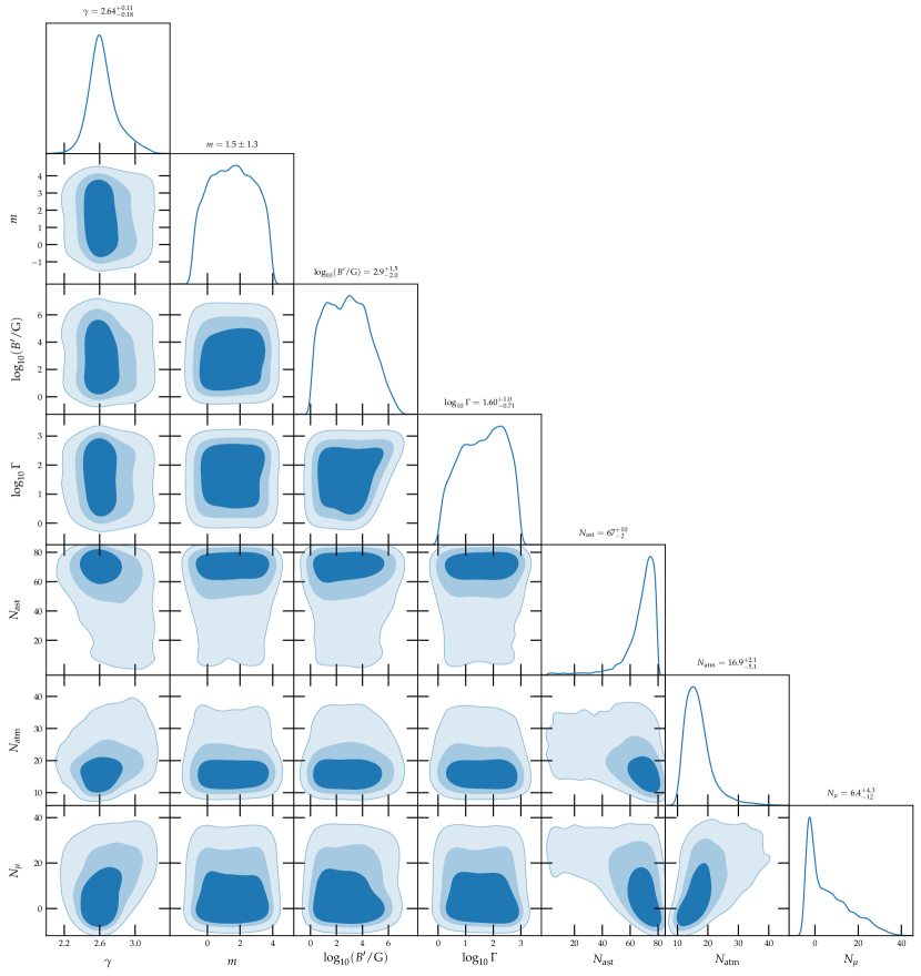
Figure A1: Posterior probability distributions, central values, and standard deviations of the likelihood parameters for the 6-year IceCube HESE sample, obtained under the signal hypothesis; see Table B1. The shaded regions show the 68%, 90%, and 95% C.L. regions, from darkest to lightest shading.

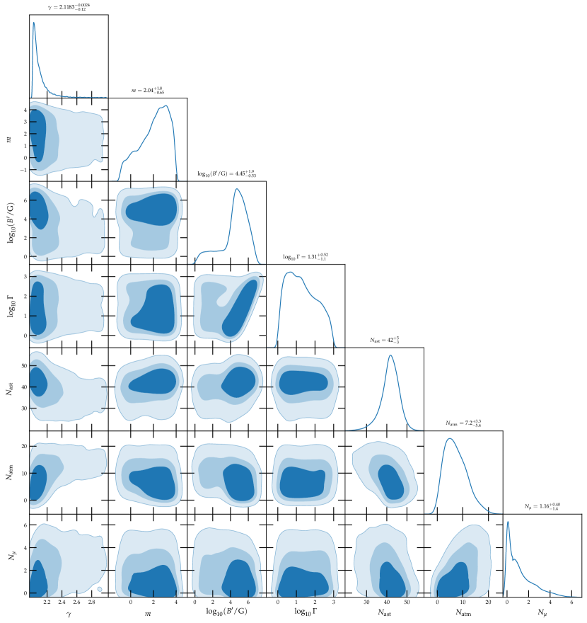
Figure A2: Same as Fig. A1, but for the 2-year IceCube MESE sample.

References

- Anchordoqui et al. (2014) L. A. Anchordoqui et al., Cosmic Neutrino Pevatrons: A Brand New Pathway to Astronomy, Astrophysics, and Particle Physics, JHEAp 1-2, 1 (2014), arXiv:1312.6587 [astro-ph.HE] .
- Aloisio (2017) R. Aloisio, Acceleration and propagation of ultra high energy cosmic rays, PTEP 2017, 12A102 (2017), arXiv:1707.08471 [astro-ph.HE] .
- Anchordoqui (2019) L. A. Anchordoqui, Ultra-High-Energy Cosmic Rays, Phys. Rept. 801, 1 (2019), arXiv:1807.09645 [astro-ph.HE] .
- Alves Batista et al. (2019) R. Alves Batista et al., Open Questions in Cosmic-Ray Research at Ultrahigh Energies, Front. Astron. Space Sci. 6, 23 (2019), arXiv:1903.06714 [astro-ph.HE] .
- Aartsen et al. (2013a) M. G. Aartsen et al. (IceCube), First observation of PeV-energy neutrinos with IceCube, Phys. Rev. Lett. 111, 021103 (2013a), arXiv:1304.5356 [astro-ph.HE] .
- Aartsen et al. (2013b) M. G. Aartsen et al. (IceCube), Evidence for High-Energy Extraterrestrial Neutrinos at the IceCube Detector, Science 342, 1242856 (2013b), arXiv:1311.5238 [astro-ph.HE] .
- Aartsen et al. (2014) M. G. Aartsen et al. (IceCube), Observation of High-Energy Astrophysical Neutrinos in Three Years of IceCube Data, Phys. Rev. Lett. 113, 101101 (2014), arXiv:1405.5303 [astro-ph.HE] .
- Aartsen et al. (2015a) M. G. Aartsen et al. (IceCube), Evidence for Astrophysical Muon Neutrinos from the Northern Sky with IceCube, Phys. Rev. Lett. 115, 081102 (2015a), arXiv:1507.04005 [astro-ph.HE] .
- Aartsen et al. (2016) M. G. Aartsen et al. (IceCube), Observation and Characterization of a Cosmic Muon Neutrino Flux from the Northern Hemisphere using six years of IceCube data, Astrophys. J. 833, 3 (2016), arXiv:1607.08006 [astro-ph.HE] .
- Bartos et al. (2017) I. Bartos, M. Ahrens, C. Finley, and S. Márka, Prospects of Establishing the Origin of Cosmic Neutrinos using Source Catalogs, Phys. Rev. D 96, 023003 (2017), arXiv:1611.03861 [astro-ph.HE] .
- Aartsen et al. (2017a) M. Aartsen et al. (IceCube), The contribution of Fermi-2LAC blazars to the diffuse TeV-PeV neutrino flux, Astrophys. J. 835, 45 (2017a), arXiv:1611.03874 [astro-ph.HE] .
- Aartsen et al. (2017b) M. Aartsen et al. (IceCube), Extending the search for muon neutrinos coincident with gamma-ray bursts in IceCube data, Astrophys. J. 843, 112 (2017b), arXiv:1702.06868 [astro-ph.HE] .
- Mertsch et al. (2017) P. Mertsch, M. Rameez, and I. Tamborra, Detection prospects for high energy neutrino sources from the anisotropic matter distribution in the local universe, JCAP 03, 011, arXiv:1612.07311 [astro-ph.HE] .
- Aartsen et al. (2019a) M. Aartsen et al. (IceCube), Search for steady point-like sources in the astrophysical muon neutrino flux with 8 years of IceCube data, Eur. Phys. J. C 79, 234 (2019a), arXiv:1811.07979 [hep-ph] .
- Murase et al. (2013) K. Murase, M. Ahlers, and B. C. Lacki, Testing the Hadronuclear Origin of PeV Neutrinos Observed with IceCube, Phys. Rev. D 88, 121301 (2013), arXiv:1306.3417 [astro-ph.HE] .
- Murase et al. (2016) K. Murase, D. Guetta, and M. Ahlers, Hidden Cosmic-Ray Accelerators as an Origin of TeV-PeV Cosmic Neutrinos, Phys. Rev. Lett. 116, 071101 (2016), arXiv:1509.00805 [astro-ph.HE] .
- Ando et al. (2015) S. Ando, I. Tamborra, and F. Zandanel, Tomographic Constraints on High-Energy Neutrinos of Hadronuclear Origin, Phys. Rev. Lett. 115, 221101 (2015), arXiv:1509.02444 [astro-ph.HE] .
- Silvestri and Barwick (2010) A. Silvestri and S. W. Barwick, Constraints on Extragalactic Point Source Flux from Diffuse Neutrino Limits, Phys. Rev. D 81, 023001 (2010), arXiv:0908.4266 [astro-ph.HE] .
- Ahlers and Halzen (2014) M. Ahlers and F. Halzen, Pinpointing Extragalactic Neutrino Sources in Light of Recent IceCube Observations, Phys. Rev. D 90, 043005 (2014), arXiv:1406.2160 [astro-ph.HE] .
- Murase and Waxman (2016) K. Murase and E. Waxman, Constraining High-Energy Cosmic Neutrino Sources: Implications and Prospects, Phys. Rev. D 94, 103006 (2016), arXiv:1607.01601 [astro-ph.HE] .
- Dekker and Ando (2019) A. Dekker and S. Ando, Angular power spectrum analysis on current and future high-energy neutrino data, JCAP 02, 002, arXiv:1811.02576 [astro-ph.HE] .
- Feyereisen et al. (2017) M. R. Feyereisen, I. Tamborra, and S. Ando, One-point fluctuation analysis of the high-energy neutrino sky, JCAP 03, 057, arXiv:1610.01607 [astro-ph.HE] .
- Aartsen et al. (2018a) M. G. Aartsen et al. (IceCube), Neutrino emission from the direction of the blazar TXS 0506+056 prior to the IceCube-170922A alert, Science 361, 147 (2018a), arXiv:1807.08794 [astro-ph.HE] .
- Stein et al. (2020) R. Stein et al., A high-energy neutrino coincident with a tidal disruption event, (2020), arXiv:2005.05340 [astro-ph.HE] .
- Kopper et al. (2016) C. Kopper, W. Giang, and N. Kurahashi (IceCube), Observation of Astrophysical Neutrinos in Four Years of IceCube Data, Proceedings of the 34th International Cosmic Ray Conference (ICRC 2015), PoS ICRC2015, 1081 (2016).
- IceCube Collaboration (2015) IceCube Collaboration, Observation of Astrophysical Neutrinos in Four Years of IceCube Data (2015 (accessed October 21, 2015)).
- Kopper (2018) C. Kopper (IceCube), Observation of Astrophysical Neutrinos in Six Years of IceCube Data, Proceedings of the 35th International Cosmic Ray Conference (ICRC 2017), PoS ICRC2017, 981 (2018).
- Aartsen et al. (2015b) M. G. Aartsen et al. (IceCube), Atmospheric and astrophysical neutrinos above 1 TeV interacting in IceCube, Phys. Rev. D 91, 022001 (2015b), arXiv:1410.1749 [astro-ph.HE] .
- IceCube Collaboration (2017) IceCube Collaboration, Search for contained neutrino events at energies greater than 1 TeV in 2 years of data (2015 (accessed September 04, 2017)).
- Arons (2003) J. Arons, Magnetars in the metagalaxy: an origin for ultrahigh-energy cosmic rays in the nearby universe, Astrophys. J. 589, 871 (2003), arXiv:astro-ph/0208444 .
- Bucciantini et al. (2008) N. Bucciantini, E. Quataert, J. Arons, B. Metzger, and T. A. Thompson, Relativistic Jets and Long-Duration Gamma-ray Bursts from the Birth of Magnetars, Mon. Not. Roy. Astron. Soc. 383, 25 (2008), arXiv:0707.2100 [astro-ph] .
- Mereghetti (2008) S. Mereghetti, The strongest cosmic magnets: Soft Gamma-ray Repeaters and Anomalous X-ray Pulsars, Astron. Astrophys. Rev. 15, 225 (2008), arXiv:0804.0250 [astro-ph] .
- Ptitsyna and Troitsky (2010) K. V. Ptitsyna and S. V. Troitsky, Physical conditions in potential sources of ultra-high-energy cosmic rays. I. Updated Hillas plot and radiation-loss constraints, Phys. Usp. 53, 691 (2010), arXiv:0808.0367 [astro-ph] .
- Ghisellini et al. (2007) G. Ghisellini, G. Ghirlanda, and F. Tavecchio, Puzzled by GRB 060218, Mon. Not. Roy. Astron. Soc. 375, L36 (2007), arXiv:astro-ph/0608555 .
- Toma et al. (2007) K. Toma, K. Ioka, T. Sakamoto, and T. Nakamura, Low-Luminosity GRB 060218: A Collapsar Jet from a Neutron Star, Leaving a Magnetar as a Remnant?, Astrophys. J. 659, 1420 (2007), arXiv:astro-ph/0610867 .
- Piran (2005) T. Piran, Magnetic Fields in Gamma-Ray Bursts: A Short Review, AIP Conf. Proc. 784, 164 (2005), arXiv:astro-ph/0503060 .
- Ghirlanda et al. (2018) G. Ghirlanda, F. Nappo, G. Ghisellini, A. Melandri, G. Marcarini, L. Nava, O. Salafia, S. Campana, and R. Salvaterra, Bulk Lorentz factors of Gamma-Ray Bursts, Astron. Astrophys. 609, A112 (2018), arXiv:1711.06257 [astro-ph.HE] .
- Ghisellini et al. (2017) G. Ghisellini, C. Righi, L. Costamante, and F. Tavecchio, The Fermi blazar sequence, Mon. Not. Roy. Astron. Soc. 469, 255 (2017), arXiv:1702.02571 [astro-ph.HE] .
- Burrows et al. (2011) D. Burrows et al., Discovery of the Onset of Rapid Accretion by a Dormant Massive Black Hole, Nature 476, 421 (2011), arXiv:1104.4787 [astro-ph.HE] .
- Thompson et al. (2006a) T. A. Thompson, E. Quataert, E. Waxman, N. Murray, and C. L. Martin, Magnetic fields in starburst galaxies and the origin of the FIR-radio correlation, Astrophys. J. 645, 186 (2006a), arXiv:astro-ph/0601626 .
- Ackermann et al. (2012) M. Ackermann et al. (Fermi-LAT), GeV Observations of Star-forming Galaxies with Fermi LAT, Astrophys. J. 755, 164 (2012), arXiv:1206.1346 [astro-ph.HE] .
- Murase et al. (2019) K. Murase, A. Franckowiak, K. Maeda, R. Margutti, and J. F. Beacom, High-Energy Emission from Interacting Supernovae: New Constraints on Cosmic-Ray Acceleration in Dense Circumstellar Environments, Astrophys. J. 874, 80 (2019), arXiv:1807.01460 [astro-ph.HE] .
- Wang et al. (2007) X.-Y. Wang, S. Razzaque, P. Mészáros, and Z.-G. Dai, High-energy Cosmic Rays and Neutrinos from Semi-relativistic Hypernovae, Phys. Rev. D 76, 083009 (2007), arXiv:0705.0027 [astro-ph] .
- Brunetti and Jones (2014) G. Brunetti and T. W. Jones, Cosmic rays in galaxy clusters and their nonthermal emission, Int. J. Mod. Phys. D 23, 1430007 (2014), arXiv:1401.7519 [astro-ph.CO] .
- Voit (2005) G. Voit, Tracing cosmic evolution with clusters of galaxies, Rev. Mod. Phys. 77, 207 (2005), arXiv:astro-ph/0410173 .
- Paliya et al. (2019) V. S. Paliya, M. Parker, J. Jiang, A. Fabian, L. Brenneman, M. Ajello, and D. Hartmann, General Physical Properties of Gamma-ray Emitting Narrow-Line Seyfert 1 Galaxies, Astrophys. J. 872, 169 (2019), arXiv:1901.07613 [astro-ph.HE] .
- Becker Tjus et al. (2014) J. Becker Tjus, B. Eichmann, F. Halzen, A. Kheirandish, and S. M. Saba, High-energy neutrinos from radio galaxies, Phys. Rev. D 89, 123005 (2014), arXiv:1406.0506 [astro-ph.HE] .
- Winter (2013) W. Winter, Photohadronic Origin of the TeV-PeV Neutrinos Observed in IceCube, Phys. Rev. D 88, 083007 (2013), arXiv:1307.2793 [astro-ph.HE] .
- Boncioli et al. (2017) D. Boncioli, A. Fedynitch, and W. Winter, Nuclear Physics Meets the Sources of the Ultra-High Energy Cosmic Rays, Sci. Rep. 7, 4882 (2017), arXiv:1607.07989 [astro-ph.HE] .
- Biehl et al. (2018a) D. Biehl, D. Boncioli, A. Fedynitch, and W. Winter, Cosmic-Ray and Neutrino Emission from Gamma-Ray Bursts with a Nuclear Cascade, Astron. Astrophys. 611, A101 (2018a), arXiv:1705.08909 [astro-ph.HE] .
- Hillas (1984) A. M. Hillas, The Origin of Ultrahigh-Energy Cosmic Rays, Ann. Rev. Astron. Astrophys. 22, 425 (1984).
- Murase and Ioka (2013) K. Murase and K. Ioka, TeV-PeV Neutrinos from Low-Power Gamma-Ray Burst Jets inside Stars, Phys. Rev. Lett. 111, 121102 (2013), arXiv:1306.2274 [astro-ph.HE] .
- Tamborra and Ando (2015) I. Tamborra and S. Ando, Diffuse emission of high-energy neutrinos from gamma-ray burst fireballs, JCAP 1509 (09), 036, arXiv:1504.00107 [astro-ph.HE] .
- Fang (2015) K. Fang, High-Energy Neutrino Signatures of Newborn Pulsars In the Local Universe, JCAP 06, 004, arXiv:1411.2174 [astro-ph.HE] .
- Carpio and Murase (2020) J. Carpio and K. Murase, Oscillation of high-energy neutrinos from choked jets in stellar and merger ejecta, Phys. Rev. D 101, 123002 (2020), arXiv:2002.10575 [astro-ph.HE] .
- Razzaque et al. (2004) S. Razzaque, P. Mészáros, and E. Waxman, TeV neutrinos from core collapse supernovae and hypernovae, Phys. Rev. Lett. 93, 181101 (2004), arXiv:astro-ph/0407064 .
- Ando and Beacom (2005) S. Ando and J. F. Beacom, Revealing the supernova-gamma-ray burst connection with TeV neutrinos, Phys. Rev. Lett. 95, 061103 (2005), arXiv:astro-ph/0502521 .
- Stecker (1979) F. W. Stecker, Diffuse Fluxes of Cosmic High-Energy Neutrinos, Astrophys. J. 228, 919 (1979).
- Kelner et al. (2006) S. R. Kelner, F. A. Aharonian, and V. V. Bugayov, Energy spectra of gamma-rays, electrons and neutrinos produced at proton-proton interactions in the very high energy regime, Phys. Rev. D 74, 034018 (2006), [Erratum: Phys. Rev. D 79, 039901 (2009)], arXiv:astro-ph/0606058 [astro-ph] .
- Kelner and Aharonian (2008) S. R. Kelner and F. A. Aharonian, Energy spectra of gamma-rays, electrons and neutrinos produced at interactions of relativistic protons with low energy radiation, Phys. Rev. D 78, 034013 (2008), arXiv:0803.0688 [astro-ph] .
- Pakvasa (2008) S. Pakvasa, Neutrino Flavor Goniometry by High Energy Astrophysical Beams, Mod. Phys. Lett. A 23, 1313 (2008), arXiv:0803.1701 [hep-ph] .
- Esteban et al. (2019) I. Esteban, M. C. Gonzalez-Garcia, A. Hernandez-Cabezudo, M. Maltoni, and T. Schwetz, Global analysis of three-flavour neutrino oscillations: synergies and tensions in the determination of , , and the mass ordering, JHEP 01, 106, arXiv:1811.05487 [hep-ph] .
- (63) NuFit, Three-neutrino fit based on data available in July 2019, http://www.nu-fit.org/.
- Aghanim et al. (2018) N. Aghanim et al. (Planck), Planck 2018 results. VI. Cosmological parameters, (2018), arXiv:1807.06209 [astro-ph.CO] .
- Tanabashi et al. (2018) M. Tanabashi et al. (Particle Data Group), Review of Particle Physics, Phys. Rev. D 98, 030001 (2018).
- Kashti and Waxman (2005) T. Kashti and E. Waxman, Flavoring astrophysical neutrinos: Flavor ratios depend on energy, Phys. Rev. Lett. 95, 181101 (2005), arXiv:astro-ph/0507599 .
- Kachelriess et al. (2008) M. Kachelriess, S. Ostapchenko, and R. Tomàs, High energy neutrino yields from astrophysical sources II: Magnetized sources, Phys. Rev. D 77, 023007 (2008), arXiv:0708.3047 [astro-ph] .
- Lipari et al. (2007) P. Lipari, M. Lusignoli, and D. Meloni, Flavor Composition and Energy Spectrum of Astrophysical Neutrinos, Phys. Rev. D 75, 123005 (2007), arXiv:0704.0718 [astro-ph] .
- Baerwald et al. (2011) P. Baerwald, S. Hümmer, and W. Winter, Magnetic Field and Flavor Effects on the Gamma-Ray Burst Neutrino Flux, Phys. Rev. D 83, 067303 (2011), arXiv:1009.4010 [astro-ph.HE] .
- Winter (2012) W. Winter, Interpretation of neutrino flux limits from neutrino telescopes on the Hillas plot, Phys. Rev. D 85, 023013 (2012), arXiv:1103.4266 [astro-ph.HE] .
- Dziewonski and Anderson (1981) A. M. Dziewonski and D. L. Anderson, Preliminary Reference Earth Model, Phys. Earth Planet. Interiors 25, 297 (1981).
- Wolfenstein (1978) L. Wolfenstein, Neutrino Oscillations in Matter, Phys. Rev. D 17, 2369 (1978).
- Mikheyev and Smirnov (1985) S. Mikheyev and A. Smirnov, Resonance Amplification of Oscillations in Matter and Spectroscopy of Solar Neutrinos, Sov. J. Nucl. Phys. 42, 913 (1985).
- Argüelles et al. (2015) C. A. Argüelles, J. Salvadó, and C. N. Weaver, A Simple Quantum Integro-Differential Solver (SQuIDS), Comput. Phys. Commun. 196, 569 (2015), arXiv:1412.3832 [hep-ph] .
- Argüelles et al. (2018a) C. A. Argüelles, J. Salvadó, and C. N. Weaver, https://github.com/jsalvado/SQuIDS/ (2018a), SQuIDS.
- Argüelles et al. (2019a) C. A. Argüelles, J. Salvadó, and C. N. Weaver, https://github.com/arguelles/nuSQuIDS (2019a), NuSQuIDS.
- Beacom and Candia (2004) J. F. Beacom and J. Candia, Shower power: Isolating the prompt atmospheric neutrino flux using electron neutrinos, JCAP 0411, 009, arXiv:hep-ph/0409046 [hep-ph] .
- Schönert et al. (2009) S. Schönert, T. K. Gaisser, E. Resconi, and O. Schulz, Vetoing atmospheric neutrinos in a high energy neutrino telescope, Phys. Rev. D 79, 043009 (2009), arXiv:0812.4308 [astro-ph] .
- Gaisser et al. (2014) T. K. Gaisser, K. Jero, A. Karle, and J. van Santen, Generalized self-veto probability for atmospheric neutrinos, Phys. Rev. D 90, 023009 (2014), arXiv:1405.0525 [astro-ph.HE] .
- Argüelles et al. (2018b) C. A. Argüelles, S. Palomares-Ruiz, A. Schneider, L. Wille, and T. Yuan, Unified atmospheric neutrino passing fractions for large-scale neutrino telescopes, JCAP 1807 (07), 047, arXiv:1805.11003 [hep-ph] .
- Tosi and Pandya (2020) D. Tosi and H. Pandya (IceCube), IceTop as veto for IceCube: results, Proceedings of the 36th International Cosmic Ray Conference (ICRC 2019), PoS ICRC2019, 445 (2020), arXiv:1908.07008 [astro-ph.HE] .
- Fedynitch et al. (2015) A. Fedynitch, R. Engel, T. K. Gaisser, F. Riehn, and T. Stanev, Calculation of conventional and prompt lepton fluxes at very high energy, Proceedings of the 18th International Symposium on Very High Energy Cosmic Ray Interactions (ISVHECRI 2014), EPJ Web Conf. 99, 08001 (2015), arXiv:1503.00544 [hep-ph] .
- Fedynitch (2019) A. Fedynitch, https://github.com/afedynitch/MCEq (2019), MCEq.
- Argüelles et al. (2019b) C. A. Argüelles, S. Palomares-Ruiz, A. Schneider, L. Wille, and T. Yuan, https://github.com/tianluyuan/nuVeto (2019b), nuVeto.
- Aartsen et al. (2015c) M. G. Aartsen et al. (IceCube), A combined maximum-likelihood analysis of the high-energy astrophysical neutrino flux measured with IceCube, Astrophys. J. 809, 98 (2015c), arXiv:1507.03991 [astro-ph.HE] .
- Palomares-Ruiz et al. (2015) S. Palomares-Ruiz, A. C. Vincent, and O. Mena, Spectral analysis of the high-energy IceCube neutrinos, Phys. Rev. D 91, 103008 (2015), arXiv:1502.02649 [astro-ph.HE] .
- Feroz and Hobson (2008) F. Feroz and M. P. Hobson, Multimodal nested sampling: an efficient and robust alternative to MCMC methods for astronomical data analysis, Mon. Not. Roy. Astron. Soc. 384, 449 (2008), arXiv:0704.3704 [astro-ph] .
- Feroz et al. (2009) F. Feroz, M. P. Hobson, and M. Bridges, MultiNest: an efficient and robust Bayesian inference tool for cosmology and particle physics, Mon. Not. Roy. Astron. Soc. 398, 1601 (2009), arXiv:0809.3437 [astro-ph] .
- Feroz et al. (2013) F. Feroz, M. P. Hobson, E. Cameron, and A. N. Pettitt, Importance Nested Sampling and the MultiNest Algorithm, (2013), arXiv:1306.2144 [astro-ph.IM] .
- Buchner et al. (2014) J. Buchner et al., X-ray spectral modelling of the AGN obscuring region in the CDFS: Bayesian model selection and catalogue, Astron. Astrophys. 564, A125 (2014), arXiv:1402.0004 [astro-ph.HE] .
- Jeffreys (1939) H. Jeffreys, The Theory of Probability, Oxford Classic Texts in the Physical Sciences (1939).
- Gupta and Zhang (2007) N. Gupta and B. Zhang, Neutrino Spectra from Low and High Luminosity Populations of Gamma Ray Bursts, Astropart. Phys. 27, 386 (2007), arXiv:astro-ph/0606744 [astro-ph] .
- Murase et al. (2006) K. Murase, K. Ioka, S. Nagataki, and T. Nakamura, High Energy Neutrinos and Cosmic-Rays from Low-Luminosity Gamma-Ray Bursts?, Astrophys. J. Lett. 651, L5 (2006), arXiv:astro-ph/0607104 .
- Kashiyama et al. (2013) K. Kashiyama, K. Murase, S. Horiuchi, S. Gao, and P. Mészáros, High energy neutrino and gamma ray transients from relativistic supernova shock breakouts, Astrophys. J. Lett. 769, L6 (2013), arXiv:1210.8147 [astro-ph.HE] .
- Senno et al. (2016) N. Senno, K. Murase, and P. Mészáros, Choked Jets and Low-Luminosity Gamma-Ray Bursts as Hidden Neutrino Sources, Phys. Rev. D 93, 083003 (2016), arXiv:1512.08513 [astro-ph.HE] .
- Zhang et al. (2018) B. T. Zhang, K. Murase, S. S. Kimura, S. Horiuchi, and P. Mészáros, Low-luminosity gamma-ray bursts as the sources of ultrahigh-energy cosmic ray nuclei, Phys. Rev. D 97, 083010 (2018), arXiv:1712.09984 [astro-ph.HE] .
- Fahey et al. (2017) S. Fahey, A. Kheirandish, J. Vandenbroucke, and D. Xu, A search for neutrinos from fast radio bursts with IceCube, Astrophys. J. 845, 14 (2017), arXiv:1611.03062 [astro-ph.HE] .
- Aartsen et al. (2018b) M. Aartsen et al. (IceCube), A Search for Neutrino Emission from Fast Radio Bursts with Six Years of IceCube Data, Astrophys. J. 857, 117 (2018b), arXiv:1712.06277 [astro-ph.HE] .
- Albert et al. (2019) A. Albert et al. (ANTARES), The search for high-energy neutrinos coincident with fast radio bursts with the ANTARES neutrino telescope, Mon. Not. Roy. Astron. Soc. 482, 184 (2019), arXiv:1807.04045 [astro-ph.HE] .
- Aartsen et al. (2019b) M. Aartsen et al. (IceCube), A Search for MeV to TeV Neutrinos from Fast Radio Bursts with IceCube 10.3847/1538-4357/ab564b (2019b), arXiv:1908.09997 [astro-ph.HE] .
- Metzger et al. (2020) B. D. Metzger, K. Fang, and B. Margalit, Neutrino Counterparts of Fast Radio Bursts, (2020), arXiv:2008.12318 [astro-ph.HE] .
- Li et al. (2014) X. Li, B. Zhou, H.-N. He, Y.-Z. Fan, and D.-M. Wei, Model-dependent estimate on the connection between fast radio bursts and ultra-high energy cosmic rays, Astrophys. J. 797, 33 (2014), arXiv:1312.5637 [astro-ph.HE] .
- Dey et al. (2016) R. K. Dey, S. Ray, and S. Dam, Searching for PeV neutrinos from photomeson interactions in magnetars, EPL 115, 69002 (2016), arXiv:1603.07833 [astro-ph.HE] .
- Andersen et al. (2020) B. Andersen et al. (CHIME/FRB), A bright millisecond-duration radio burst from a Galactic magnetar, (2020), arXiv:2005.10324 [astro-ph.HE] .
- Ridnaia et al. (2020) A. Ridnaia et al., A peculiar hard X-ray counterpart of a Galactic fast radio burst, (2020), arXiv:2005.11178 [astro-ph.HE] .
- Bochenek et al. (2020) C. D. Bochenek, V. Ravi, K. V. Belov, G. Hallinan, J. Kocz, S. R. Kulkarni, and D. L. McKenna, A fast radio burst associated with a Galactic magnetar, (2020), arXiv:2005.10828 [astro-ph.HE] .
- Tavani et al. (2020) M. Tavani et al., An X-Ray Burst from a Magnetar Enlightening the Mechanism of Fast Radio Bursts, (2020), arXiv:2005.12164 [astro-ph.HE] .
- Zhang et al. (2003) B. Zhang, Z. Dai, and P. Mészáros, High-energy neutrinos from magnetars, Astrophys. J. 595, 346 (2003), arXiv:astro-ph/0210382 .
- Waxman and Bahcall (1997) E. Waxman and J. N. Bahcall, High-energy neutrinos from cosmological gamma-ray burst fireballs, Phys. Rev. Lett. 78, 2292 (1997), arXiv:astro-ph/9701231 [astro-ph] .
- Murase and Nagataki (2006) K. Murase and S. Nagataki, High energy neutrino emission and neutrino background from gamma-ray bursts in the internal shock model, Phys. Rev. D 73, 063002 (2006), arXiv:astro-ph/0512275 [astro-ph] .
- Hümmer et al. (2012) S. Hümmer, P. Baerwald, and W. Winter, Neutrino Emission from Gamma-Ray Burst Fireballs, Revised, Phys. Rev. Lett. 108, 231101 (2012), arXiv:1112.1076 [astro-ph.HE] .
- Zhang and Kumar (2013) B. Zhang and P. Kumar, Model-dependent high-energy neutrino flux from Gamma-Ray Bursts, Phys. Rev. Lett. 110, 121101 (2013), arXiv:1210.0647 [astro-ph.HE] .
- Liu and Wang (2013) R.-Y. Liu and X.-Y. Wang, Diffuse PeV neutrinos from gamma-ray bursts, Astrophys. J. 766, 73 (2013), arXiv:1212.1260 [astro-ph.HE] .
- Baerwald et al. (2015) P. Baerwald, M. Bustamante, and W. Winter, Are gamma-ray bursts the sources of ultra-high energy cosmic rays?, Astropart. Phys. 62, 66 (2015), arXiv:1401.1820 [astro-ph.HE] .
- Tamborra and Ando (2016) I. Tamborra and S. Ando, Inspecting the supernova–gamma-ray-burst connection with high-energy neutrinos, Phys. Rev. D 93, 053010 (2016), arXiv:1512.01559 [astro-ph.HE] .
- Stecker et al. (1991) F. W. Stecker, C. Done, M. H. Salamon, and P. Sommers, High-energy neutrinos from active galactic nuclei, Phys. Rev. Lett. 66, 2697 (1991).
- Atoyan and Dermer (2001) A. Atoyan and C. D. Dermer, High-energy neutrinos from photomeson processes in blazars, Phys. Rev. Lett. 87, 221102 (2001), arXiv:astro-ph/0108053 [astro-ph] .
- Murase et al. (2012a) K. Murase, C. D. Dermer, H. Takami, and G. Migliori, Blazars as Ultra-High-Energy Cosmic-Ray Sources: Implications for TeV Gamma-Ray Observations, Astrophys. J. 749, 63 (2012a), arXiv:1107.5576 [astro-ph.HE] .
- Padovani and Resconi (2014) P. Padovani and E. Resconi, Are both BL Lacs and pulsar wind nebulae the astrophysical counterparts of IceCube neutrino events?, Mon. Not. Roy. Astron. Soc. 443, 474 (2014), arXiv:1406.0376 [astro-ph.HE] .
- Kimura et al. (2015) S. S. Kimura, K. Murase, and K. Toma, Neutrino and Cosmic-Ray Emission and Cumulative Background from Radiatively Inefficient Accretion Flows in Low-Luminosity Active Galactic Nuclei, Astrophys. J. 806, 159 (2015), arXiv:1411.3588 [astro-ph.HE] .
- Padovani et al. (2015) P. Padovani, M. Petropoulou, P. Giommi, and E. Resconi, A simplified view of blazars: the neutrino background, Mon. Not. Roy. Astron. Soc. 452, 1877 (2015), arXiv:1506.09135 [astro-ph.HE] .
- Cerruti et al. (2019) M. Cerruti, A. Zech, C. Boisson, G. Emery, S. Inoue, and J.-P. Lenain, Leptohadronic single-zone models for the electromagnetic and neutrino emission of TXS 0506+056, Mon. Not. Roy. Astron. Soc. 483, L12 (2019), arXiv:1807.04335 [astro-ph.HE] .
- Liu et al. (2019) R.-Y. Liu, K. Wang, R. Xue, A. M. Taylor, X.-Y. Wang, Z. Li, and H. Yan, Hadronuclear interpretation of a high-energy neutrino event coincident with a blazar flare, Phys. Rev. D 99, 063008 (2019), arXiv:1807.05113 [astro-ph.HE] .
- Palladino et al. (2019) A. Palladino, X. Rodrigues, S. Gao, and W. Winter, Interpretation of the diffuse astrophysical neutrino flux in terms of the blazar sequence, Astrophys. J. 871, 41 (2019), arXiv:1806.04769 [astro-ph.HE] .
- Keivani et al. (2018) A. Keivani et al., A Multimessenger Picture of the Flaring Blazar TXS 0506+056: implications for High-Energy Neutrino Emission and Cosmic Ray Acceleration, Astrophys. J. 864, 84 (2018), arXiv:1807.04537 [astro-ph.HE] .
- Murase et al. (2018) K. Murase, F. Oikonomou, and M. Petropoulou, Blazar Flares as an Origin of High-Energy Cosmic Neutrinos?, Astrophys. J. 865, 124 (2018), arXiv:1807.04748 [astro-ph.HE] .
- Gao et al. (2019) S. Gao, A. Fedynitch, W. Winter, and M. Pohl, Modelling the coincident observation of a high-energy neutrino and a bright blazar flare, Nature Astron. 3, 88 (2019), arXiv:1807.04275 [astro-ph.HE] .
- Rodrigues et al. (2019) X. Rodrigues, S. Gao, A. Fedynitch, A. Palladino, and W. Winter, Leptohadronic Blazar Models Applied to the 2014–2015 Flare of TXS 0506+056, Astrophys. J. Lett. 874, L29 (2019), arXiv:1812.05939 [astro-ph.HE] .
- Petropoulou et al. (2020) M. Petropoulou et al., Multi-Epoch Modeling of TXS 0506+056 and Implications for Long-Term High-Energy Neutrino Emission, Astrophys. J. 891, 115 (2020), arXiv:1911.04010 [astro-ph.HE] .
- Fang and Metzger (2017) K. Fang and B. D. Metzger, High-Energy Neutrinos from Millisecond Magnetars formed from the Merger of Binary Neutron Stars, Astrophys. J. 849, 153 (2017), arXiv:1707.04263 [astro-ph.HE] .
- Fang et al. (2016) K. Fang, K. Kotera, K. Murase, and A. V. Olinto, IceCube Constraints on Fast-Spinning Pulsars as High-Energy Neutrino Sources, JCAP 04, 010, arXiv:1511.08518 [astro-ph.HE] .
- Smith et al. (2020) D. Smith, D. Hooper, and A. Vieregg, Revisiting AGN as the Source of IceCube’s Diffuse Neutrino Flux, (2020), arXiv:2007.12706 [astro-ph.HE] .
- Anchordoqui et al. (2004) L. A. Anchordoqui, H. Goldberg, F. Halzen, and T. J. Weiler, Neutrino bursts from Fanaroff-Riley I radio galaxies, Phys. Lett. B 600, 202 (2004), arXiv:astro-ph/0404387 .
- Stecker (2005) F. W. Stecker, A Note on High Energy Neutrinos from AGN Cores, Phys. Rev. C 72, 107301 (2005), arXiv:astro-ph/0510537 .
- Álvarez-Muñiz and Mészáros (2004) J. Álvarez-Muñiz and P. Mészáros, High energy neutrinos from radio-quiet AGNs, Phys. Rev. D 70, 123001 (2004), arXiv:astro-ph/0409034 .
- Stecker (2013) F. W. Stecker, PeV neutrinos observed by IceCube from cores of active galactic nuclei, Phys. Rev. D 88, 047301 (2013), arXiv:1305.7404 [astro-ph.HE] .
- Hooper et al. (2019) D. Hooper, T. Linden, and A. Vieregg, Active Galactic Nuclei and the Origin of IceCube’s Diffuse Neutrino Flux, JCAP 02, 012, arXiv:1810.02823 [astro-ph.HE] .
- Dai and Fang (2017) L. Dai and K. Fang, Can tidal disruption events produce the IceCube neutrinos?, Mon. Not. Roy. Astron. Soc. 469, 1354 (2017), arXiv:1612.00011 [astro-ph.HE] .
- Lunardini and Winter (2017) C. Lunardini and W. Winter, High Energy Neutrinos from the Tidal Disruption of Stars, Phys. Rev. D 95, 123001 (2017), arXiv:1612.03160 [astro-ph.HE] .
- Biehl et al. (2018b) D. Biehl, D. Boncioli, C. Lunardini, and W. Winter, Tidally disrupted stars as a possible origin of both cosmic rays and neutrinos at the highest energies, Sci. Rep. 8, 10828 (2018b), arXiv:1711.03555 [astro-ph.HE] .
- Winter and Lunardini (2020) W. Winter and C. Lunardini, A concordance scenario for the observation of a neutrino from the Tidal Disruption Event AT2019dsg, (2020), arXiv:2005.06097 [astro-ph.HE] .
- Murase et al. (2020) K. Murase, S. S. Kimura, B. T. Zhang, F. Oikonomou, and M. Petropoulou, High-Energy Neutrino and Gamma-Ray Emission from Tidal Disruption Events, (2020), arXiv:2005.08937 [astro-ph.HE] .
- Loeb and Waxman (2006) A. Loeb and E. Waxman, The Cumulative background of high energy neutrinos from starburst galaxies, JCAP 0605, 003, arXiv:astro-ph/0601695 [astro-ph] .
- Stecker (2007) F. W. Stecker, Are Diffuse High Energy Neutrinos from Starburst Galaxies Observable?, Astropart. Phys. 26, 398 (2007), arXiv:astro-ph/0607197 .
- Thompson et al. (2006b) T. A. Thompson, E. Quataert, E. Waxman, and A. Loeb, Assessing The Starburst Contribution to the Gamma-Ray and Neutrino Backgrounds, (2006b), arXiv:astro-ph/0608699 [astro-ph] .
- He et al. (2013) H.-N. He, T. Wang, Y.-Z. Fan, S.-M. Liu, and D.-M. Wei, Diffuse PeV neutrino emission from ultraluminous infrared galaxies, Phys. Rev. D 87, 063011 (2013), arXiv:1303.1253 [astro-ph.HE] .
- Tamborra et al. (2014) I. Tamborra, S. Ando, and K. Murase, Star-forming galaxies as the origin of diffuse high-energy backgrounds: Gamma-ray and neutrino connections, and implications for starburst history, JCAP 1409, 043, arXiv:1404.1189 [astro-ph.HE] .
- Chang and Wang (2014) X.-C. Chang and X.-Y. Wang, The diffuse gamma-ray flux associated with sub-PeV/PeV neutrinos from starburst galaxies, Astrophys. J. 793, 131 (2014), arXiv:1406.1099 [astro-ph.HE] .
- Peretti et al. (2020) E. Peretti, P. Blasi, F. Aharonian, G. Morlino, and P. Cristofari, Contribution of starburst nuclei to the diffuse gamma-ray and neutrino flux, Mon. Not. Roy. Astron. Soc. 493, 5880 (2020), arXiv:1911.06163 [astro-ph.HE] .
- Horiuchi and Ando (2008) S. Horiuchi and S. Ando, High-energy neutrinos from reverse shocks in choked and successful relativistic jets, Phys. Rev. D 77, 063007 (2008), arXiv:0711.2580 [astro-ph] .
- Murase (2018) K. Murase, New Prospects for Detecting High-Energy Neutrinos from Nearby Supernovae, Phys. Rev. D 97, 081301 (2018), arXiv:1705.04750 [astro-ph.HE] .
- Petropoulou et al. (2017) M. Petropoulou, S. Coenders, G. Vasilopoulos, A. Kamble, and L. Sironi, Point-source and diffuse high-energy neutrino emission from Type IIn supernovae, Mon. Not. Roy. Astron. Soc. 470, 1881 (2017), arXiv:1705.06752 [astro-ph.HE] .
- Senno et al. (2018) N. Senno, K. Murase, and P. Mészáros, Constraining high-energy neutrino emission from choked jets in stripped-envelope supernovae, JCAP 01, 025, arXiv:1706.02175 [astro-ph.HE] .
- Esmaili and Murase (2018) A. Esmaili and K. Murase, Constraining high-energy neutrinos from choked-jet supernovae with IceCube high-energy starting events, JCAP 12, 008, arXiv:1809.09610 [hep-ph] .
- Fang et al. (2020a) K. Fang, B. D. Metzger, I. Vurm, E. Aydi, and L. Chomiuk, High-Energy Neutrinos and Gamma-Rays from Non-Relativistic Shock-Powered Transients, (2020a), arXiv:2007.15742 [astro-ph.HE] .
- Villante and Vissani (2008) F. Villante and F. Vissani, How precisely neutrino emission from supernova remnants can be constrained by gamma ray observations?, Phys. Rev. D 78, 103007 (2008), arXiv:0807.4151 [astro-ph] .
- Liu et al. (2014) R.-Y. Liu, X.-Y. Wang, S. Inoue, R. Crocker, and F. Aharonian, Diffuse PeV neutrinos from EeV cosmic ray sources: Semirelativistic hypernova remnants in star-forming galaxies, Phys. Rev. D 89, 083004 (2014), arXiv:1310.1263 [astro-ph.HE] .
- Chakraborty and Izaguirre (2015) S. Chakraborty and I. Izaguirre, Diffuse neutrinos from extragalactic supernova remnants: Dominating the 100 TeV IceCube flux, Phys. Lett. B 745, 35 (2015), arXiv:1501.02615 [hep-ph] .
- Dar and Shaviv (1996) A. Dar and N. J. Shaviv, The Extragalactic neutrino background radiations from blazars and cosmic rays, Astropart. Phys. 4, 343 (1996), arXiv:astro-ph/9504083 .
- Berezinsky et al. (1997) V. S. Berezinsky, P. Blasi, and V. S. Ptuskin, Clusters of Galaxies as a Storage Room for Cosmic Rays, Astrophys. J. 487, 529 (1997), arXiv:astro-ph/9609048 [astro-ph] .
- De Marco et al. (2006) D. De Marco, P. Blasi, P. Hansen, and T. Stanev, High energy neutrinos from cosmic ray interactions in clusters of galaxies, Phys. Rev. D 73, 043004 (2006), arXiv:astro-ph/0511535 [astro-ph] .
- Kotera et al. (2009) K. Kotera, D. Allard, K. Murase, J. Aoi, Y. Dubois, T. Pierog, and S. Nagataki, Propagation of ultrahigh energy nuclei in clusters of galaxies: resulting composition and secondary emissions, Astrophys. J. 707, 370 (2009), arXiv:0907.2433 [astro-ph.HE] .
- Zandanel et al. (2015) F. Zandanel, I. Tamborra, S. Gabici, and S. Ando, High-energy gamma-ray and neutrino backgrounds from clusters of galaxies and radio constraints, Astron. Astrophys. 578, A32 (2015), arXiv:1410.8697 [astro-ph.HE] .
- Senno et al. (2015) N. Senno, P. Mészáros, K. Murase, P. Baerwald, and M. J. Rees, Extragalactic star-forming galaxies with hypernovae and supernovae as high-energy neutrino and gamma-ray sources: the case of the 10 TeV neutrino data, Astrophys. J. 806, 24 (2015), arXiv:1501.04934 [astro-ph.HE] .
- Capel et al. (2020) F. Capel, D. J. Mortlock, and C. Finley, Bayesian constraints on the astrophysical neutrino source population from IceCube data, Phys. Rev. D 101, 123017 (2020), arXiv:2005.02395 [astro-ph.HE] .
- Fang et al. (2020b) K. Fang, A. Banerjee, E. Charles, and Y. Omori, A Cross-Correlation Study of High-energy Neutrinos and Tracers of Large-Scale Structure, Astrophys. J. 894, 112 (2020b), arXiv:2002.06234 [astro-ph.HE] .
- Waxman and Bahcall (1999) E. Waxman and J. N. Bahcall, High energy neutrinos from astrophysical sources: An upper bound, Phys. Rev. D59, 023002 (1999), arXiv:hep-ph/9807282 .
- Mannheim et al. (2001) K. Mannheim, R. J. Protheroe, and J. P. Rachen, On the cosmic ray bound for models of extragalactic neutrino production, Phys. Rev. D63, 023003 (2001), arXiv:astro-ph/9812398 .
- Mücke et al. (2000) A. Mücke, R. Engel, J. Rachen, R. Protheroe, and T. Stanev, SOPHIA: Monte Carlo simulations of photohadronic processes in astrophysics, Comput. Phys. Commun. 124, 290 (2000), arXiv:astro-ph/9903478 [astro-ph] .
- Hümmer et al. (2010) S. Hümmer, M. Rüger, F. Spanier, and W. Winter, Simplified models for photohadronic interactions in cosmic accelerators, Astrophys. J. 721, 630 (2010), arXiv:1002.1310 [astro-ph.HE] .
- Anchordoqui et al. (2008) L. A. Anchordoqui, D. Hooper, S. Sarkar, and A. M. Taylor, High-energy neutrinos from astrophysical accelerators of cosmic ray nuclei, Astropart. Phys. 29, 1 (2008), arXiv:astro-ph/0703001 .
- Petropoulou (2014) M. Petropoulou, The role of hadronic cascades in GRB models of efficient neutrino production, Mon. Not. Roy. Astron. Soc. 442, 3026 (2014), arXiv:1405.7669 [astro-ph.HE] .
- Morejón et al. (2019) L. Morejón, A. Fedynitch, D. Boncioli, D. Biehl, and W. Winter, Improved photomeson model for interactions of cosmic ray nuclei, JCAP 11, 007, arXiv:1904.07999 [astro-ph.HE] .
- Murase et al. (2012b) K. Murase, K. Asano, T. Terasawa, and P. Mészáros, The Role of Stochastic Acceleration in the Prompt Emission of Gamma-Ray Bursts: Application to Hadronic Injection, Astrophys. J. 746, 164 (2012b), arXiv:1107.5575 [astro-ph.HE] .
- Winter et al. (2014) W. Winter, J. Becker Tjus, and S. R. Klein, Impact of secondary acceleration on the neutrino spectra in gamma-ray bursts, Astron. Astrophys. 569, A58 (2014), arXiv:1403.0574 [astro-ph.HE] .
- Aartsen et al. (2020) M. Aartsen et al. (IceCube-Gen2), IceCube-Gen2: The Window to the Extreme Universe, (2020), arXiv:2008.04323 [astro-ph.HE] .
- Bustamante et al. (2015) M. Bustamante, J. F. Beacom, and W. Winter, Theoretically palatable flavor combinations of astrophysical neutrinos, Phys. Rev. Lett. 115, 161302 (2015), arXiv:1506.02645 [astro-ph.HE] .
- Dulat et al. (2016) S. Dulat, T.-J. Hou, J. Gao, M. Guzzi, J. Huston, P. Nadolsky, J. Pumplin, C. Schmidt, D. Stump, and C. Yuan, New parton distribution functions from a global analysis of quantum chromodynamics, Phys. Rev. D 93, 033006 (2016), arXiv:1506.07443 [hep-ph] .
- Bustamante et al. (2020) M. Bustamante, C. Rosenstrøm, S. Shalgar, and I. Tamborra, Bounds on secret neutrino interactions from high-energy astrophysical neutrinos, Phys. Rev. D 101, 123024 (2020), arXiv:2001.04994 [astro-ph.HE] .
- Bustamante (2020) M. Bustamante, New limits on neutrino decay from the Glashow resonance of high-energy cosmic neutrinos, (2020), arXiv:2004.06844 [astro-ph.HE] .