25mm25mm25mm25mm

Resumo
Large Fluctuations in Stochastic Models of Turbulence
Gabriel Brito Apolinário
Orientador: Luca Moriconi
Resumo da Tese de Doutorado apresentada ao Programa de Pós-Graduação em Física do Instituto de Física da Universidade Federal do Rio de Janeiro - UFRJ, como parte dos requisitos necessários à obtenção do título de Doutor em Ciências (Física).

As primeiras observações de flutuações estatísticas em turbulência, descritas pelas equações de Navier-Stokes, foram feitas na década de 1940 e já revelavam a presença de intermitência: Distribuições de probabilidade de caudas largas em observáveis como gradientes de velocidade, diferenças de velocidade, e dissipação de energia. Hoje em dia, com experimentos cada vez mais precisos e simulações numéricas em números de Reynolds cada vez maiores, reitera-se as observações de grandes flutuações, mas uma descrição teórica que conecta as equações de Navier-Stokes à estatística observada ainda é um problema em aberto. Esta tese discute o fenômeno da intermitência em três modelos de turbulência, se valendo de técnicas analíticas e numéricas para a análise de processos estocásticos e as distribuições estatísticas que estes geram.

Os capítulos iniciais apresentam uma revisão da teoria estatística da turbulência e da teoria estatística de campos aplicada à física fora do equilíbrio. É discutida a história das equações de Navier-Stokes e a necessidade de uma formulação estocástica destas para explicar os fenômenos da turbulência. Em seguida, os sucessos e limitações da fenomenologia de Kolmogorov de 1941 são apresentados. A principal dessas limitações é não incluir os efeitos das flutuações, que são ponto central da teoria de Kolmogorov-Obukhov e da teoria multifractal, abordadas em seguida. Também é feita uma revisão dos métodos funcionais aplicados a sistemas de equações diferenciais estocásticas.

O modelo Recent Fluid Deformation (RFD), que descreve a dinâmica de gradientes de velocidade lagrangeanos, e o modelo de Burgers, que descreve a formação de ondas de choque em fluidos unidimensionais, são investigados através do método funcional Martin-Siggia-Rose-Janssen-de Dominicis (MSRJD). Nesta formulação, os instantons (soluções das equações de Euler-Lagrange obtidas a partir da ação de MSRJD) já tinham sido identificados como a contribuição principal à distribuição de probabilidade de gradientes de velocidade nos dois modelos. Nesta tese é feita uma análise cuidadosa das hipóteses e resultados que levaram a essas observações anteriores sobre os instantons e sobre correções perturbativas correspondentes a flutuações nos dois modelos.

No caso do RFD, é feita uma contagem de potências dos diagramas perturbativos associados às flutuações ao redor dos instantons e uma verificação da validade do instanton aproximado usado em cálculos anteriores. No modelo de Burgers, foram identificados dois diagramas perturbativos até segunda ordem na expansão em cumulantes, que são cruciais para entender um procedimento ad hoc de renormalização já observado em discussões anteriores: A distribuição de probabilidade gerada pelos instantons descreve bem as distribuições de probabilidade numéricas, mas é necessário adicionar um fator de correção ao parâmetro que regula a intensidade das flutuações. Foi investigada a contribuição das flutuações para induzir esse fator de correção.

Por último, é apresentado um processo estocástico estacionário e unidimensional como um modelo das flutuações da pseudo-dissipação lagrangeana. Esse processo apresenta ruído aleatório na escala microscópica, construído a partir de um processo multifractal discreto, assim como uma dinâmica regular em escalas ainda menores. Foram verificadas as propriedades estatísticas desse processo aleatório, que apresenta uma distribuição de probabilidade lognormal, e correlações de longo alcance na forma de leis de potência, de acordo com as propriedades estatísticas experimentais da pseudo-dissipação.

Palavras-chave: Turbulência, modelos estocásticos, eventos extremos, formalismo Martin-Siggia-Rose, renormalização.

Abstract
Large Fluctuations in Stochastic Models of Turbulence
Gabriel Brito Apolinário
Orientador: Luca Moriconi
Abstract da Tese de Doutorado apresentada ao Programa de Pós-Graduação em Física do Instituto de Física da Universidade Federal do Rio de Janeiro - UFRJ, como parte dos requisitos necessários à obtenção do título de Doutor em Ciências (Física).

The first observations of statistical fluctuations in turbulence, described by the Navier-Stokes equations, were made in decade of 1940 and already revealed the presence of intermittency: The probability distribution functions of observables such as velocity gradients, velocity differences and kinetic energy dissipation are heavy tailed. Nowadays, with more precise experiments and numerical simulations at larger Reynolds numbers, the observations of large fluctuations are reinforced, but a theoretical description that connects the Navier-Stokes equations to the observed statistics is still an open problem. This dissertation discusses the intermitency phenomenon in three models of turbulence, employing analytical and numerical techniques in the analysis of stochastic processes and the probability distributions which they induce.

The initial chapters present a review of the statistical theory of turbulence and of statistical theory of fields as applied to out of equilibrium physics. The history of the Navier-Stokes equation is discussed and associated to the need for a stochastic formulation of them in order to explain turbulent phenomena. Then, the successes and limitations of the Kolmogorov 1941 phenomenology are presented. The predominant limitation is not to include fluctuation effects, the central point of the Kolmogorov-Obukhov and multifractal theories, which are reviewed. A summary of functional methods applied to systems of stochastic differential equations is also presented.

The RFD model, which describes the dynamics of Lagrangian velocity gradients, and the Burgers model, describing the formation of shock waves in one-dimensional fluids, are investigated through the Martin-Siggia-Rose-Janssen-de Dominicis (MSRJD) functional method. In this formulation, the instantons (solutions of the Euler-Lagrange equations obtained from the MSRJD action) had already been identified as the leading contribution to the velocity gradient probability distribution function in both models. In this dissertation, a careful analysis of the previous hypothesis and results is undertaken, in order to verify the observations of perturbative corrections corresponding to fluctuations around the instanton in both models.

In the Recent Fluid Deformation (RFD) model, a power-counting procedure on the perturbative diagrams associated to fluctuations around the instantons is pursued, along with a validation of the approximate instanton used in prior calculations. In the Burgers model, two perturbative diagrams were identified up to second order in the cumulant expansion. They are revealed to be crucial in understanding an ad hoc renormalization procedure reported in the literature: The probability distribution induced by the instantons describes velocity gradient fluctuations well, if a correction factor is added to the parameter associated to the intensity of fluctuations. The contribution of fluctuations to cause this correction factor is investigated.

In the end, a stationary one-dimensional stochastic process is presented as a model of Lagrangian pseudo-dissipation fluctuations. This model displays random noise in the microscopic scale, built from a discrete multifractal process, but at smaller scales its dynamics is regular. The statistical properties of this random process are verified, and it is observed that, in agreement with established properties of the pseudo-dissipation, this process has a lognormal probability distribution and long range power-law correlations.

Keywords: Turbulence, stochastic models, extreme events, Martin-Siggia-Rose formalism, renormalization.

Agradecimentos

Agradeço aos meus pais pelo apoio e pela confiança ao longo destes anos de estudo. Nada disso seria possível sem esse incentivo e amparo.

Pelo aprendizado sobre a prática da ciência, que inclui as técnicas, a leitura, a escrita, as discussões e o pensamento crítico, e pelos riquíssimos problemas científicos que me propôs, agradeço ao Prof. Luca Moriconi.

Agradeço também aos companheiros semanais no journal club de turbulência e dinâmica de fluidos, Rodrigo Arouca, Elvis Soares, Bruno Magacho, Victor Valadão, Mirlene Oliveira, Marina Moesia e Maiara Neumann. E agradeço ao Rodrigo Pereira pela valiosa colaboração, e pelos ensinamentos em programação.

Agradeço aos novos amigos que fiz nesse período na UFRJ, aos amigos de longa data da UFF, e aos amigos que fiz nas viagens, ao longo do doutorado. Vinicius Henning, Pedro Foster, Reginaldo Junior, Luis Fernando, Rodrigo Bruni, Kainã Diniz, Flavianna Siller, Lucas Hutter, Lucas Torres, Patrícia Abrantes, Larissa Inácio, Ethe Costa, Evelyn Caso, Daniel Martin, Irene Lamberti, Fabiana Monteiro, Humberto Medeiros, Gleice Germano, Leonardo Pio, Ruslan Guerra: Obrigado.

Aos funcionários Igor Silva, Khrisna Teixeira, César Chagas e Mariana Sampaio, agradeço pelo apoio em questões técnicas e administrativas. E à Luana Serpa pela ajuda com o catálogo da exposição “Turbulência e Arte” e as respectivas fotos que abrem alguns dos capítulos.

Por fim, agradeço ao CNPq pelo surporte financeiro, sem o qual este doutoramento não teria sido possível.

List of Abbreviations

DNS	Direct Numerical Simulation
LHS	Left-hand side
MSRJD	Martin-Siggia-Rose-Janssen-de Dominicis
PDF	Probability Density Function
RFD	Recent Fluid Deformation
RHS	Right-hand side
SDE	Stochastic Differential Equation
SPDE	Stochastic Partial Differential Equation

Chapter 1 Introduction

In the beginning of the XXth century, the Isar Company of Munich had the task of building banks for the Isar River, to prevent it from flooding. They contacted Arnold Sommerfeld with the question: At what point would the river flow change from smooth (laminar) to irregular (turbulent)? Sommerfeld and Werner Heisenberg, then, performed an analysis of the equations of flow and predicted a limit of stability for the smooth solution. As a follow-up to this story, there is an apocryphal quote attributed to Heisenberg (cited by [15]:

When I meet God, I am going to ask him two questions. Why relativity? And why turbulence? I really believe he will have an answer for the first.

The same citation has been attributed as well to Richard Feynman and to Horace Lamb, and relativity is sometimes replaced with quantum electrodynamics. For more details on these stories, the reader is referred to [15, 57].

This tale illustrates the lasting interest that turbulence has had as a scientific problem, both in pure and applied research. Turbulent flows are ubiquitous in daily and industrial flows, such as the atmosphere, the ocean, combustion engines and wind tunnels. It is easy to imagine that mankind has tried to understand and control it since the beginning of science. The first theoretical contributions to this problem came from the founders of classical mechanics: Newton, Euler, Bernoulli, Lagrange, Navier and Stokes, among others, who determined the equations which dictate the evolution of velocity and pressure in viscous and inviscid flows, respectively the Navier-Stokes equation and the Euler equation.

The modern understanding of the problem only came with the experiments and theories developed in the XX century, by scientists such as Osborne Reynolds (1842-1912), Geoffrey I. Taylor (1886-1975), Lewis Fry Richardson (1881-1953), Ludwig Prandtl (1875-1953) and Theodore von Kármán (1881-1963), who described the phenomena of the laminar-turbulent transition, the formation of vortical structures, the energy cascade and the boundary layer. Their contributions served as inspirations to theorists such as Andrey Kolmogorov (1903-1987), Lev Landau (1908-1968) and Lars Onsager (1903-1976), who built the first models to describe these phenomena and still inspire much of the current developments in this research area.

The Navier-Stokes and Euler equations have attracted the interest of mathematicians, as well, for they provide seemingly simple equations, but with complex nonlinearities, still not fully understood. Even the basic problem of existence and smoothness of solutions of these equations remains open. This is a famous open problem in mathematics, one of the Millenium Prize Problems, with a US$ 1 million prize offered by the Clay Mathematics Institute for its solution. The formal statement asks for a proof of existence (or non-existence) of global regularity in the Navier-Stokes equations. In other words, if starting with smooth initial conditions, do the velocity and pressure fields remain regular and analytical for any finite time or do they develop singularities?

The global regularity problem is also open for the Euler equation in three dimensions, but partial results in different settings have been obtained. For Navier-Stokes in two dimensions, regularity was proven in [129]. In three dimesions, the existence of weak solutions to the Navier-Stokes equations was proved in [138] (weak solutions are briefly discussed in Sec. 2.6). A rigorous description of this problem can be found in [72], and a mathematical discussion of the theory of turbulence is available in [216].

Figure 1.1: Large scale numerical simulation of a turbulent flow from [107]. Intense vorticity isosurfaces are depicted, the vorticity is displayed if it deviates more than four standard deviations from the mean. Clouds of small eddies interleaved with void regions can be seen, illustrating the non-homogeneity of turbulent fiels.

Another area of study with rich interactions with turbulence is that of numerical simulations of partial differential equations. Various numerical schemes for their solution have been developed, most notably the spectral methods, which rely on fast algorithms for the numerical Fourier transform to obtain higher precision than would be possible with numerical simulations of the same size in real space. Spectral methods were first applied in turbulence in [173], on a grid of $32^{3}$ points, and have evolved to simulations with $16\ 384^{3}$ points [110], where very detailed structures can be identified. This is illustrated in Fig. 1.1, extracted from [107]. In this work, snapshots of a simulation with $4096^{3}$ grid points are shown, and structures such as vortex tubes are clearly seen.

Notable as well is the importance that the study of turbulence has on technological applications. In some industrial areas, it is desired to suppress turbulence, such as in flows through pipes, where the external pressure difference applied to the ends of the pipe is greatly reduced, for a fixed flow rate, if the fluid is calm and laminar, rather than irregular and turbulent. In other situations turbulence is beneficial, for instance in the efficient mix of chemical reactants, where turbulent flows vastly accelerate the dispersal of chemicals and the occurrence of reactions. For a review of engineering problems and turbulence, the reader is referred to [50, 219].

To summarize, the prominent features of turbulent flows, which permit us to understand the challenges in their study and the potential for applications are:

1. enhanced energy dissipation, even in the limit of vanishing viscosity;

2. strong mixing of energy, momentum, mass and heat;

3. unpredictability of flow configurations.

A discussion of these properties is pursued in Chap. 2, where the statistical theory of turbulence is discussed, and the topics investigated in this dissertation are different manifestations of these phenomena. The inclusion of this general discussion has the objective of making this text self-contained and accessible to researchers and students unfamiliar with the topic, since the theory of turbulence is seldom included in graduation curricula. The content of the review chapter is based on the discussions of [78, 75, 158, 63] with references to further sources.

Chap. 3 is, likewise, a review on the theory of stochastic calculus, functional methods and instantons, where its history and some techniques are discussed. These techniques are employed in the next chapters, which cover the original contributions discussed in this dissertation. In this chapter, the discussion is mostly based on [85, 92, 32].

In Chap. 4, Lagrangian turbulence and statistical closures are introduced, along with a discussion of the results of [6]. To predict transport properties, such as mixing and spread of dispersed particles, it is necessary to understand Lagrangian velocity gradients, but the equation for their dynamics, derived from the Navier-Stokes equations, is unclosed. Consequently, many closure approximations have been developed, particularly the Recent Fluid Deformation (RFD), in [39], which was investigated with functional methods in [160]. An extension of these analytical results is pursued in two ways: A hierarchical classification of perturbative contributions is performed and the most relevant diagrams are integrated into the renormalized effective action. The approximate instanton hypothesis is also verified to be true.

The next chapter, 5, discusses the onset of intermittency in Burgers turbulence along the lines of the functional formalism. The Burgers model is a one-dimensional version of the Navier-Stokes equation, which shares many qualitative features with the original model, hence it is sometimes used as test case for analytical and numerical techniques in turbulence. For this equation, the relevance of the instanton approach in the description of large fluctuations of the velocity gradient has been verified in previous works [93]. Nevertheless, it was also revealed the need of an empirical noise renormalization. In [7], on which this chapter is based, a theoretical explanation for the mechanism of noise renormalization is presented.

In Chap. 6, a different route is taken in the investigation of Lagrangian pseudo-dissipation. A stochastic differential equation with a stationary solution is used to model the fluctuations of this observable. This stochastic process is driven by shot noise, a periodic and discrete source of randomness, inspired by the discrete and exactly multifractal causal process described in [180]. It is verified that this discrete dynamics leads to multifractal statistics and long-range correlations compatible with known models of pseudo-dissipation. This chapter is based on [5].

Chapter 2 Statistical Theory of Turbulence

The pursuit of a complete statistical theory of turbulence has been singular for some reasons. Its phenomena have been recognized since ancient times, yet a descriptive approach which stems from the Navier-Stokes equations, and derives the results known nowadays still seems far from being realized. The most successful attempts have been to build phenomenological theories, and their use was aptly described by Feynman, talking about superfluidity:

Rather than look at the Hamiltonian we shall “wave our hands”, use analogies with simpler systems, draw pictures, and make plausible guesses based on physical intuition to obtain a qualitative picture of the solutions (wave functions). This qualitative approach will prove singularly successful. [73, p.321]

Just as described, the theory of turbulence has relied strongly on physical pictures and analogies. One of the main ideas that have inspired the construction of theories, and forms the basic picture of turbulence, is the energy cascade. First stated in [191], it described turbulent flows as composed of eddies of different sizes, ranging from the largest scales in the flow to the smallest. Kinetic energy is injected into the flow at the large scales, through the external force, and generates large vortices, which are unstable and break up. Energy is then transferred progressively and without loss to smaller eddies, that go through the same breakup process. After reaching the smallest scales, energy is finally dissipated by viscosity. This process is illustrated in Fig. 2.1

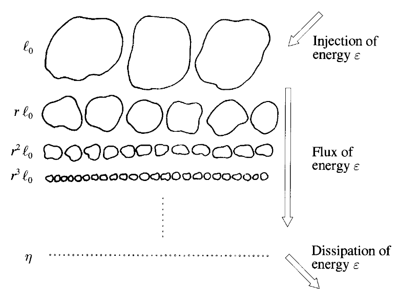
Figure 2.1: The Richardson cascade is illustrated in this figure from [78]. Vortices of different scales are shown, from the integral scale down to the dissipative scale. The transference of kinetic energy across scales is local and inviscid, that is, the same amount of energy being is transferred between neighboring scales at every step.

The cascade picture was the basic inspiration of Kolmogorov in building his theory, which proposed a self-similar velocity field as approximate solution to the Navier-Stokes equations. The approach of Kolmogorov was to incorporate experimental and theoretical knowledge into a theory in order to build a consistent framework from which further predictions could be made. Some of these predictions are the scaling behavior of statistical observables, such as velocity differences, energy dissipation and enstrophy. All of these observables will be defined in later sections.

From the energy cascade picture, a large separation of scales can be inferred. The energy containing range is placed in one end of the spectrum, the large scale, and the dissipation range in the other end, the small scale. This separation of scales also induces the idea of scale invariance of some observables, which, together with its anomalous breaking, is one of the main ingredients of the current understanding of turbulent flows.

2.1 The Navier-Stokes Equations

Fluids are treated as a continuous medium, despite the knowledge, confirmed in the beginning of the XX century that matter is made of atoms and is discontinuous. A successful continuum description relies on the large separation between the molecular scale (set by the mean free path of the molecules of the fluid, $\lambda$) and the typical scales of the flow (the integral scale $L$, defined by the external force on the fluid and by the geometry). In quantitative terms, the Knudsen number, $\mathrm{Kn}=\lambda/L$, must satisfy $\mathrm{Kn}\ll 1$ for a valid continuum formulation. In this regime, the fluid can be described by quantities which vary with continuous position and time indexes: A single instant of a flow is characterized by its density, velocity and pressure at each point. This is called the Eulerian point of view in fluid dynamics, in which the coordinates refer to a fixed reference frame. There is also the Lagrangian frame, in which individual parcels of fluid are tracked, and the position index refers to the position of this “fluid particle” in the initial time. By “fluid particle” it is not meant a molecule, but an amount of fluid which can be treated as an individual particle, it is much smaller than all relevant scales in the flow, yet much larger than the mean free path of its molecules. This is only possible because of the large separation of scales.

Fluid dynamics is then the result of applying conservation of mass, energy and momentum to a continuous medium. Mass conservation in this context is also called the equation of continuity:

$$\partial_{t}\rho+\partial_{i}(\rho u_{i})=0\ .$$ (2.1)

Notice that, in this equation and in the rest of this dissertation, latin indices stand for spatial coordinates, ranging from one to three. Derivatives with respect to time are represented by $\partial_{t}$ and derivatives with respect to space coordinate $x_{i}$ by $\partial_{i}$. And the Einstein convention for summation over repeated indices is adopted, unless otherwise specified.

Momentum conservation is written through Newton’s second law, in terms of the acceleration $\gamma_{i}$, at a certain point, and the Cauchy stress tensor $\sigma_{ij}$, which describes the interaction of different fluid parcels with each other:

$$\rho\gamma_{i}=\partial_{j}\sigma_{ij}+f_{i}\ ,$$ (2.2)

where $f_{i}$ is an external, divergenceless, body force, acting on the whole fluid, with a possible dependence on position and time. The acceleration is the material derivative of velocity:

$$\gamma_{i}=Du_{i}/Dt=\partial_{t}u_{i}+u_{j}\partial_{j}u_{i}\ .$$ (2.3)

The material derivative of the velocity is the acceleration experienced by a particle moving with the flow, which is different from the acceleration of the velocity at this point ($\partial_{t}u_{i}$).

The material derivative computes the time rate of change of any quantity such as temperature or velocity (which gives acceleration) for a portion of a material moving with a velocity, v. If the material is a fluid, then the movement is simply the flow field.

To proceed further, some knowledge of the properties of the fluid, modelled through the $\sigma_{ij}$ tensor, is needed. The simplest model for the stress tensor is a linear dependence on velocity, which describes a Newtonian fluid:

$$\sigma_{ij}=\mu(\partial_{j}u_{i}+\partial_{i}u_{j})+(\lambda\partial_{m}u_{m}-p)\delta_{ij}\ .$$ (2.4)

The variable $p$ is the pressure and it varies with position and time, and the constants $\mu$ and $\lambda$ are specific to each fluid, $\mu$ is the molecular (or dynamic) viscosity coefficient, and $3\lambda+2\mu$ is called the viscous dilatation coefficient. The linear form was proposed by Newton, who also performed the first experiments to measure the viscosity coefficient. Eq. 2.4 is the most straightforward model of a viscous fluid, capturing the behavior of actual substances such as air and water remarkably well in most quotidian or industrial situations [128].

In these common settings, a useful approach is to consider the typical speeds in the flow much smaller than the speed of sound in the medium. In this limit, spatial differences in density adjust quickly compared to the motion of the fluid, which means the density can be considered constant in the whole flow. Such a flow is called incompressible. In this special situation, Eq. (2.1) is altered to:

$$\partial_{i}u_{i}=0\ ,$$ (2.5)

and this is called the incompressibility condition. In turn, this also simplifies Eq. (2.4):

$$\sigma_{ij}=\mu(\partial_{j}u_{i}+\partial_{i}u_{j})-p\delta_{ij}\ .$$ (2.6)

With the above expressions the Navier-Stokes equations for incompressible flows are obtained:

$$\partial_{t}u_{i}+u_{j}\partial_{j}u_{i}=-\frac{1}{\rho}\partial_{i}p+\frac{\mu}{\rho}\partial^{2}u_{i}\ ,$$ (2.7)

where $\partial^{2}$ represents the Laplacian operator, $\partial_{i}\partial_{i}$. Since the density is constant, it is customary to rewrite

$$p/\rho\to p\qquad\mbox{and}\qquad\mu/\rho\to\nu\ ,$$ (2.8)

where $\nu$ is called the kinematic viscosity. Its value is known for all common fluids and is more directly relevant to applications than the dynamic viscosity. As an example, the kinematic viscosity of water at 20ºC is $1.00\times 10^{-6}$ m²/s and $1.51\times 10^{-5}$ m²/s for air at 20ºC (see [61] and [60]). These values are not so distant from each other, despite the difference in the respective dynamic viscosity of nearly three decades.

Under the change of variables in Eq. (2.8), the incompressible Navier-Stokes equations become:

$$\begin{split}\partial_{t}u_{i}+u_{j}\partial_{j}u_{i}&=-\partial_{i}p+\nu\partial^{2}u_{i}+f_{i}\ ,\\ \partial_{i}u_{i}&=0\ .\end{split}$$ (2.9)

A complete description of a fluid dynamical requires these equations, together with an initial condition for the velocity field, and the no-slip boundary condition: the velocity of the fluid at the boundaries is always null.

The no-slip boundary condition was proposed by Stokes, who performed experiments in fluids and found no slip velocity. Later, a kinetic theory argument was used by Maxwell to demonstrate that the slip velocity is of the order of magnitude of the mean free path of the molecules of the fluid, hence for macroscopic fluids, the no-slip boundary condition is well-suited. More details on this topic can be found in [49, 204] and in [63, Chap.6].

Observe that the incompressibility condition renders the pressure field non-local. This effect can be seen by deriving the Navier-Stokes equations with respect to coordinate $i$ and obtaining

$$\partial^{2}p=-(\partial_{i}u_{j})(\partial_{j}u_{i})\ ,$$ (2.10)

which is the Poisson equation. It can be solved with the use of Green’s functions and its solution for $p$ at each point is an integral over the whole domain, hence is it nonlocal. This already illustrates some of the difficulties in determining mathematical solutions to the Navier-Stokes equations.

2.2 Reynolds Similarity

Important contributions to the phenomenology of turbulence came from the British scientist Osborne Reynolds (1842 - 1912), who performed paramount experiments in this subject. Many of the methods developed by him at this time have a direct connection with modern experimental techniques for visualization of flows. Reynolds investigated flows on long pipes, which be seen in Fig. 2.2, in drawings from his notebooks. Using small jets of dyed water introduced into the center of the flow and electric sparks, he could visualize structures in the motion of water in the pipe.

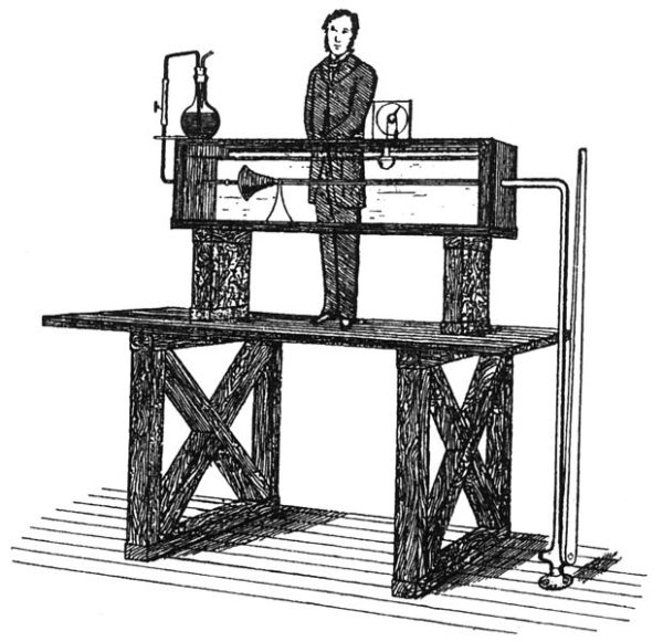
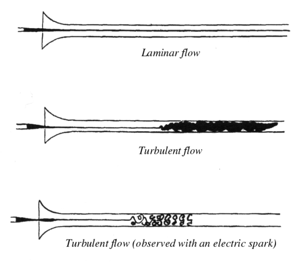
Figure 2.2: The original drawings of [189] describe his experimental apparatus: A long pipe, in the middle of which a jet of dyed water was inserted. A valve allowed him to control the input velocity of the fluid, and thus demonstrate the transition from a laminar state to a turbulent flow. With an electric spark, vortical structures in the pipe could also be visualized.

In an experiment from 1883, he demonstrated the transition of a flow from an ordered state to another which is irregular and unpredictable. The first is called a laminar flow, because different streams in the fluid seem to form independent layers, barely interacting with each other. And the latter is a turbulent flow. It displays complex swirly patterns, called vortices, which mix all layers of the stream. A flow control valve was used to regulate the inlet velocity of water in the tube and Reynolds noticed that, as the velocity increases, the behavior of the flow changes from the laminar to the turbulent state.

The scientist also noticed that a single dimensionless number is responsible for this transition. In his memory this parameter of the flow is called the Reynolds number, defined as

$$\mathrm{Re}=UL/\nu\ .$$ (2.11)

In this definition, $U$ and $L$ are respectively a typical velocity and length in the flow, and $\nu$ is the kinematic viscosity, which can be measured for each different fluid. The typical velocity may be defined by the inlet velocity of the fluid, or its mean velocity in the flow. And the typical length is usually defined by the geometry, such as the length of the boundaries containing the flow, or by the characteristic length of the external force.

The concept of the Reynolds number only gained popularity after these experiments, but it was introduced theoretically in 1851 by George Stokes (for a discussion on the history of the Reynolds number, [193] should be consulted). Stokes noticed that, in the Navier-Stokes equations, there is only one relevant dimensionless parameter. The relevance of the Reynolds number may be noticed by rewriting the Navier-Stokes equations in dimensionless form, with the following changes of variables:

$$\partial_{t}=\frac{U}{L}\partial_{t}^{\prime}\ ,\quad\partial_{i}=\frac{1}{L}\partial_{i}^{\prime}\ ,\quad u=Uu^{\prime}\ ,\quad p=U^{2}p^{\prime}\quad\mbox{and}\quad f=\frac{U^{2}}{L}f^{\prime}\ ,$$ (2.12)

with the same typical scales $U$ and $L$ as in Eq. (2.11).

After these transformations, the Navier-Stokes equations become:

$$\partial_{t}^{\prime}u_{i}^{\prime}+u_{j}^{\prime}\partial_{j}^{\prime}u_{i}^{\prime}=-\partial_{i}^{\prime}p^{\prime}+\frac{1}{\mathrm{Re}}\partial^{\prime 2}u_{i}^{\prime}+f_{i}^{\prime}\ ,$$ (2.13)

with the Reynolds number as defined in Eq. (2.11). It can be seen that, in the regime of high Reynolds number, the dissipation term $\partial^{\prime 2}u_{i}^{\prime}/\mathrm{Re}$ becomes less relevant in comparison with the nonlinear term. On the contrary, when the Reynolds number is very small, dissipation gains relevance relative to the inertial contribution.

A simple dimensional argument exists to reinforce this conclusion: Looking at the flow only at a characteristic scale $\ell$, the nonlinear term has a typical intensity $u^{2}/\ell$, and the dissipative term, in turn, has a typical dimension $u/(\ell^{2}\mbox{Re})$. At large scales, the nonlinear term prevails, and creates complex vortical structures in the flow, even if the initial state is smooth. And at small scales, the dissipation term dominates, and acts in order to smooth out these turbulent structures.

Nevertheless, one could naively imagine, from this argument, that viscous forces can be ignored at large Reynolds numbers. But ignoring the viscous contribution changes the Navier-Stokes equations from second order in the spatial derivatives to only first order, and this change renders impossible the realization of the no-slip boundary condition. Therefore, there is an abrupt difference in behavior between the case of vanishing viscosity (very large Reynolds) and the case of exactly zero viscosity (corresponding to the Euler equations). In the first situation, fluid motion is highly turbulent, whereas in the second there can be laminar solutions irrespective of any scale of the flow. This abrupt change is a singular limit.

Consequently, one should tread with care in using a scaling argument, for their validity is restricted to intermediate length scales, far from the injection or dissipation scales, illustrated in the cascade picture. This regime of intermediate length scales is called the inertial range, and a more precise description of it is given in Sec. 2.5. A scale-based analysis, though, can be made rigorous and is a useful tool in studies of turbulence. Several mathematical and numerical techniques decompose turbulent flows according to their scales of motion, such as Fourier analysis, wavelet methods and coarse-graining in real space. For more details, the reader is referred to [71, 177].

The singular limit is also responsible for the formation of the boundary layer in wall flows, such as flows around airplanes and ships, or over a landscape. There is a strong mean component in these flows, which are often treated as idealized and frictionless (solutions of the Euler equation), but near the walls rapid variations of velocity and the appearance of complex vortical structures occur, which cannot be understood without the viscous contribution. This phenomenon, the boundary layer, is of great relevance to engineering applications, as can be imagined. On this topic, the reader is referred to [201].

2.3 The Random External Force

In the experiments on turbulent flows, such as those performed by Reynolds, one of the first features that was noticed was the seemingly random nature of the solutions. The same phenomenon happens in numerical simulations of the Navier-Stokes equations: Minute differences in the initial or boundary conditions, or small instabilities due to truncation errors in the numerical routines, generate solutions which, after some time, look nothing like each other. This is also one of the main features of chaotic systems, discovered in [141], a parallel which has led to numerous investigations on the connection between turbulence and chaos [64, 25, 22].

Quantitative evidence on the effect of small perturbations in turbulence have been investigated, for instance, through the dispersion of particle pairs in turbulent flows since [192]. This work describes several experiments with particles in atmospheric flows, and its main result, called the Richardson dispersion law, describes the growth of the mean square distance of two particles in a turbulent flow:

$$\langle r^{2}\rangle\propto t^{3}\ .$$ (2.14)

This result shows that the dispersion of trajectories in turbulent flows is superdiffusive: Much faster than in Brownian motion, in which $\langle r^{2}\rangle\propto t$. In the case of Brownian motion, though, the path taken by the particles is completely uncorrelated and memoryless, and to explain Eq. (2.14), the complex correlations in time and space of turbulent fields have to be taken into account. Modern verifications of this law can be found in [26, 28, 195].

Nevertheless, chaotic behavior is characterized by an exponential separation of trajectories, rather than the algebraic growth of Eq. (2.14). It has been argued that at small scales (the dissipative range), particles separate exponentially fast [83, 239], while in the inertial range, separation is algebraic, given by Richardson’s dispersion. The algebraic separation is an altogether different phenomenon which produces randomness in turbulent flows. Velocity fields in turbulent flows are irregular and not continuously differentiable, which leads to the phenomenon of spontaneous stochasticity of Lagrangian trajectories: Only a statistical description of these trajectories is possible, since the equations describing their evolution display multiple solutions. This phenomenon and Richardson’s dispersion law are deeply linked, as observed in [24, 66]. The first description of spontaneous stochasticity were presented in [24, 87, 86], and a rigorous proof in the context of advection by a random field (the Kraichnan model) was presented in [136]. More details on these topics are available in [66, 63]. The roughness of the turbulent velocity field is also further discussed in Sec. 2.6.

Due to this inevitable randomness, both from the recent theories, and from the early observations of unpredictable behavior, it is common in theoretical and numerical investigations to define the external force $f_{i}$ in the Navier-Stokes equations, Eq. (2.9), as a random source of Gaussian nature, with zero mean, correlated on the large scales and delta-correlated in time. This is formally described as

$$\begin{split}\langle f_{i}(\mathbf{r},t)\rangle&=0\ ,\\ \langle f_{i}(\mathbf{r},t)f_{j}(\mathbf{r^{\prime}},t^{\prime})\rangle&=\chi(|\mathbf{r}-\mathbf{r^{\prime}})|)\delta(t-t^{\prime})\delta_{ij}\ .\end{split}$$ (2.15)

In this equation, $\delta(t)$ is the Dirac delta function and $\delta_{ij}$ is the Kronecker delta symbol. $\chi(r)$ is the correlation function of the external force, its characteristic length is $L$ and this function decays fast at distances larger than $L$.

In this manner, the observed randomness is produced artificially. But the statistical properties of the resulting flow are expected to be the same for two main reasons. The first, of a physical nature, is that flows at very high Reynolds numbers display universal behavior, particularly the exponents of statistical moments of Galilean invariant quantities. The second reason is in connection with the theory of dynamical systems: Birkhoff’s theorem shows that, for ergodic systems, there is an underlying probability distribution which reproduces its statistical features, even if the original dynamical system is deterministic [78, 43].

Resorting to Birkhoff’s theorem requires the assumption that turbulence is ergodic. In experiments, measurements are often made of time-averaged quantities. Theoretical considerations, on the other side, rely on ensemble averages, which are equivalent to averages over some probability distribution function. To connect the experimental and theoretical results, ergodicity has also been proposed without proof. It is important to mention that the same assumption has to be made in many other systems, in equilibrium or not, since there are few problems where a proof of ergodicity exists. One of these is the hard sphere billiard, its ergodicity was proven in [206].

Studies of the Navier-Stokes equations as a dynamical system have been pursued since [130, 102], and a mathematical foundation has been established for the rigorous meaning of the ensemble average and the statistics of a turbulent stationary state. For a discussion of these results, the reader is referred to [82, 75]. With the availability of large scale numerical simulations, where both time and ensemble averages can be calculated, numerical verifications of ergodicity have also been done, in [84], supporting the hypothesis.

All of these considerations are drawn as basis for the use of a stochastic version of the Navier-Stokes equations and its variants, although an explanation of the clear connection between noise and Navier-Stokes dynamics is still missing [63].

2.4 Symmetries of Fluid Dynamical Equations

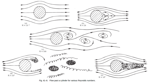
Figure 2.3: This image, extracted from [74], depicts the flow past a cylinder. It starts regular at low Reynolds numbers, this is the laminar flow, shown in the top left. At higher values of Re, instabilities set in and periodic solutions, with rotating vortices arise, this is the von Karman vortex street, shown in the middle. With even higher Re, the flow becomes turbulent, a situation in which all layers of the flow are mixed, seen in the bottom right. The Reynolds number is the only parameter that governs this transition in typical flows.

Since few exact results can be drawn directly from the Navier-Stokes equations, an analysis of its symmetries becomes all the more relevant to the study of turbulence. In Fig. 2.3, a drawing from [74] depicts the flow around a cylinder at increasing Reynolds numbers, a setting where symmetries and symmetry breaking can be recognized.

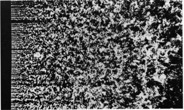
Figure 2.4: In this image from [223], homogeneous turbulence is generated by a flow incoming from the left and impinging on a rectangular grid. This setting can be used to study the properties of homogeneous isotropic turbulence, since, far from the grid, the large scale features of the flow are weaker.

At small Reynolds numbers, this flow is stationary, which means it is invariant under time translations. As the Reynolds increases, instabilities develop and rotating vortices appear behind the cylinder, breaking time translation to a discrete symmetry. These vortices alternate between swirling with the flow and against it, in a periodic manner, but in this situation, the behavior of the flow is still orderly and predictable. At even higher Reynolds numbers (Fig. 2.3d), this periodicity is lost and random vortices begin to populate the flow. The last state, (Fig. 2.3e), at the highest Reynolds number, is called fully developed turbulence. Invariance under time translations is hopeless in this situation, as are attempts at predicting the future state of the flow, due to its irregular behavior. But in a statistical description, since it is observed that stationarity is recovered when looking at ensemble averages. This is what is meant by a stationary flow: The statistical symmetry of translation in time of an ensemble of similarly prepared flows.

A similar phenomenon happens regarding spatial symmetries. The presence of the cylinder makes translational invariance seem impossible, since it does not exist even at small Reynolds numbers. Nevertheless, there is such a symmetry if one looks at the small scales of the turbulent flow in Fig. 2.3e. Away from the boundaries and at such small length scales, the overall properties of the flow lose relevance. Then, spatial symmetries are recovered in this limit: Both rotational and translational invariance, in a statistical sense, are properties of the fully turbulent flow

Another setup, which is commonly used in experiments, is turbulence generated by a spatial grid, illustrated in Fig. 2.4. In the figure, the fluid is flowing from left to right and at the left side there is a regular grid. The unpredictable properties of the flow quickly manifest behind the grid, where individual streaks of flow, coming out of the empty spacings, start to mix. The pattern generated away from the grid does not inherit any of the symmetries of the setup, and instead displays statistical invariance under translations and rotation. The name given to a statistical invariance under translations is homogeneity, and to statistical invariance under rotations, isotropy.

These symmetries are manifest in all flows at sufficiently high Reynolds numbers, and at small scales, irrespective of the symmetries of the external force or the geometry of the flow. For this reason, the basic paradigm in the study of turbulence are the properties of stationary, homogeneous and isotropic flows. This is the simplest configuration of a turbulent flow, and the view of restored symmetries provides a theoretical vindication to studying such flows.

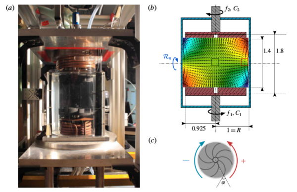
Figure 2.5: This figure, extracted from [53], displays an experimental setup for the generation of von Karman flows (a). In (b) and (c), details of the working of the rotating paddles are shown. The black and red boxes in the (b) are the two regions observed in the experiments, one in the middle of the flow, where mixing from several layers of flow generates turbulence which is very accurately homogeneous and isotropic, and one very close to the boundary layer, yet the statistical observations are equivalent in this region.

An experimental setup which is very commonly used to generate homogeneous isotropic turbulence is shown in Fig. 2.5: two counter-rotating propellers at the bottom and the top impel the motion of fluid. In the middle plane of the setup, there is a mixing layer. Measurements in the mixing layer display all properties of homogeneous and isotropic flows with good accuracy. Recent experiments with this arrangement have reached Reynolds numbers of the order of $10^{5}$ [47].

The statistical symmetries are inherited from the global symmetries of the Navier-Stokes equations, which are more than simply time translations, spatial translations and rotations. And they form the basis of the modern view of Kolmogorov’s theory. Some of these symmetries are only observed in the regime of infinite Reynolds (equivalent to vanishing viscosity). This is called the inviscid regime, and it corresponds formally to the Euler equation:

$$\begin{split}\partial_{t}u_{i}+u_{j}\partial_{j}u_{i}&=-\partial_{i}p\ ,\\ \partial_{i}u_{i}=0\ .\end{split}$$ (2.16)

As discussed, this is a singular limit, and strong qualitative differences exist in the solutions of the Euler equation, often smooth and symmetric, and the Navier-Stokes equation at vanishing viscosity, corresponding to fully developed turbulence. But at intermediate length scales, where the dissipative (viscous) effects can be ignored, the symmetries of the Euler equation are relevant in the study of fully developed viscous flows.

Then, the global symmetries of the Euler equations are the following:

1. Space translations: $t,r_{i},v_{i}(\bm{r},t)\to t,r_{i}+\rho_{i},v_{i}(\bm{r},t)$

2. Time translations: $t,r_{i},v_{i}(\bm{r},t)\to t+\tau,r_{i},v_{i}(\bm{r},t)$

3. Galilean transformations: $t,r_{i},v_{i}(\bm{r},t)\to t,r_{i}+U_{i}\ t,v_{i}(\bm{r},t)+U_{i}$

4. Parity: $t,r_{i},v_{i}(\bm{r},t)\to t,-r_{i},-v_{i}(\bm{r},t)$

5. Rotations: $t,r_{i},v_{i}(\bm{r},t)\to t,\Lambda_{ij}r_{j},\Lambda_{ij}v_{j}(\bm{r},t)$, where $\Lambda\in SO(3)$.

6. Time reversal: $t,r_{i},v_{i}(\bm{r},t)\to-t,r_{i},-v_{i}(\bm{r},t)$

7. Scaling: $t,r_{i},v_{i}(\bm{r},t)\to\lambda^{1-h}t,\lambda r_{i},\lambda^{h}v_{i}(\bm{r},t)$, $\lambda>0$ and $h$ is a real number.

Proofs can be found in [158]. The last two are symmetries exclusively of the Euler equation, while the others are symmetries of the Navier-Stokes equation as well.

Applying the time reversal transformations (item 6 above) to the Navier-Stokes equations, it can be noticed that the term responsible for breaking this symmetry is the viscous contribution, $\nu\partial^{2}u_{i}$. This is one more evidence that the viscous term is responsible for the system being dissipative, and for this reason there is no symmetry under time reversal.

Regarding the last symmetry, the Euler equations are invariant under any $h$ rescaling, whereas the Navier-Stokes equation are only invariant under rescaling if $h=-1$. Nonetheless, the symmetries in the Navier-Stokes equations are not necessarily manifest in the solutions, as can be observed in the flows of Fig. 2.5.

These symmetries inspired Kolmogorov to build a theory based on three basic hypothesis. In the next sections, these hypothesis and their limitations are going to be discussed.

2.5 The Theory of 1941

Andrey Kolmogorov was one the most important mathematicians of the twentieth century. He was responsible for the modern development of the theory of probability and of turbulence, along with paramount contributions in areas such as topology, logics, classical mechanics and computational complexity. In 1941, he published three articles which laid the foundations for the statistical theory of turbulence: [121, 122, 123]. For this reason they form what is called the K41 theory.

The picture of the energy cascade inspired Kolmogorov to build three hypotheses as the basis of a phenomenological theory of fully developed turbulence. At the time, these hypotheses were formulated in terms of universality of statistical observables at sufficiently high Reynolds numbers. In this text, instead, the point of view of restored symmetries is adopted. This is a contemporary interpretation of the Kolmogorov hypotheses, described in [78]. Both interpretations are equivalent, portaying the same theory, but the symmetry perspective enables to investigate more deeply their range of validity and limitations. These hypotheses are still some of the foundations of the statistical theory of turbulence, even with all the posterior developments. They operate as good approximations to reality in the limit of infinite Reynolds number, at small scales and away from boundaries. Their statement follows.

The first hypothesis of K41 is that, under the given assumptions, all possible symmetries of the Navier-Stokes equations are statistically restored. As was discussed in Sec. 2.4, these symmetries are usually broken by the mechanisms producing the turbulent flow. The key point in this hypothesis is that the details of the large scale forcing and flow boundaries lose relevance in the infinite Reynolds limit.

Under the same assumptions, the second hypothesis states that a turbulent flow is self-similar at small scales. This means the flow possesses a unique scaling exponent $h$, such that the velocity is a statistically self-similar field:

$$\delta\mathbf{v}(\mathbf{r},\lambda\ell)\overset{d}{=}\lambda^{h}\delta\mathbf{v}(\mathbf{r},\ell)\ .$$ (2.17)

In this equation, $\delta\mathbf{v}(\mathbf{r},\ell)=\mathbf{v}(\mathbf{r}+\ell\mathbf{x})-\mathbf{v}(\mathbf{r})$ is the velocity difference along the direction of $\mathbf{x}$. The equality in distribution in Eq. (2.17), indicated by $\overset{d}{=}$, means that both sides follow the same probability distribution. Hence, this is not a strict equality, but only a statistical correspondence, valid when an ensemble of flows is considered.

Finally, the third hypothesis, valid under the same assumptions, is that turbulent flows have a finite nonvanishing mean rate of kinetic energy dissipation per unit mass. This quantity is denoted by the symbol $\varepsilon$. This means that, if the integral scale $L$ and the large scale velocity $U$ are kept constant, and the limit $\nu\to 0$ is taken, $\varepsilon$ reaches a constant, non-zero, value.

Overall, these hypotheses define the general statistical features of the velocity field in a turbulent flow. For instance, this explains why all turbulent flows display the same statistical features at small scales, regardless of the specific geometry of the flow, or the forcing conditions.

An equivalent dimensional argument, which Kolmogorov employed, is that the only dimensional quantities which influence the flow at small scales are the mean energy dissipation $\varepsilon$ and the kinematic viscosity $\nu$. From these quantities, a single characteristic length scale can be built. It is a microscopic length called the Kolmogorov scale,

$$\eta_{K}=(\nu^{3}/\varepsilon)^{1/4}\ .$$ (2.18)

At this scale, dissipation gains relevance relative to the nonlinear advection, and the vortices are smoothed out of the flow. For this reason, the scales below $\eta_{K}$ are called the dissipative range. If the Reynolds number is large enough, there is a large difference between the small scale $\eta_{K}$ and the large scale $L$. In the intermediate scale, the relevance of both the large scale effects (anisotropy) and the small scale effects (dissipation) can be discarded, and universal behavior is observed. With a precise definition of the dissipation scale, the inertial range also receives a more rigorous characterization: It contains the length scales $\ell$ such that $\eta_{K}\ll\ell\ll L$. The statistical hypotheses of Kolmogorov were designed to describe turbulent fields in this interval, where neither dissipation nor large scale geometry are relevant, thus the flow properties may only depend on a single property: the kinetic energy dissipation, $\varepsilon$.

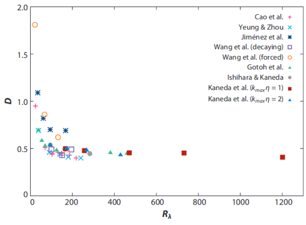
Figure 2.6: This figure, extracted from [107], displays the nondimensionalized energy dissipation for several different numerical simulations. The energy dissipation, made dimensionless by the respective input parameters of each simulation, evolve to the same constant value as the Reynolds number increases.

The rate of dissipation $\varepsilon$ is constant across scales, since energy loss only occurs in the dissipative range. Therefore, the value of $\varepsilon$ can be determined from the large scale features, where vortices have a typical kinetic energy of $U^{2}$ and a turnover time scale of $T=L/U$. Then, the energy transfer rate per unit mass is dimensionally equivalent to $K/T=U^{3}/L$. The constant of proportionality between the actual value of the energy dissipation and $U^{3}/L$ is expected to be a universal quantity, independent on the flow, in the infinite Reynolds limit. This property, referred to as the zeroth law of turbulence, or dissipative anomaly, was first discussed in [52], and in the reformulation of the K41 theory in terms of restored symmetries, pursued in [77], it enters as the third hypothesis. Several measurements, both in experiments and numerical simulations, have been made and they support this claim, as can be seen in Fig. 2.6. For discussions on this topic, the reader is referred to [31, 209, 211, 176, 116].

In the sections that follow, the main results of the Kolmogorov 1941 theory of turbulence are going to be introduced. These results follow from the basic hypothesis together with manipulations of the Navier-Stokes equations.

2.5.1 The Energy Budget Equation

From the Navier-Stokes equations, an equation which describes the flow of energy can be written: The energy budget equation. This equation provides a quantitative aspect to the cascade picture, in which energy is transported in an inviscid manner from the large to the small scales. It can be obtained by taking a scalar product of Eq. (2.9) with $u_{i}$. Then, an average of the result produces the desired equation:

$$\big{\langle}u_{i}\partial_{t}u_{i}\big{\rangle}+\big{\langle}u_{j}u_{i}\partial_{j}u_{i}\big{\rangle}=\nu\big{\langle}u_{i}\partial^{2}u_{i}\big{\rangle}-\big{\langle}u_{i}\partial_{i}p\big{\rangle}+\big{\langle}f_{i}u_{i}\big{\rangle}\ .$$ (2.19)

The angle brackets indicate a spatial average, that is, an integral over the whole domain $\Omega$ of the flow:

$$\langle f\rangle=\frac{\int_{\Omega}d\mathbf{r}\ f(\mathbf{r})}{\int_{\Omega}d\mathbf{r}}\ .$$ (2.20)

For this reason, the rule of integration by parts, which will be used extensively, applies directly to the averaged function. The first term of Eq. (2.19) is a derivative of the energy density (per unit mass). This can be seen by rewriting the first term as:

$$\big{\langle}u_{i}\partial_{t}u_{i}\big{\rangle}=\frac{1}{2}\big{\langle}\partial_{t}|u_{i}|^{2}\big{\rangle}=\frac{d}{dt}\mathcal{T}(\mathbf{u})\ ,$$ (2.21)

where $\mathcal{T}(\mathbf{u})$ is the energy density:

$$\mathcal{T}(\mathbf{u})=\frac{1}{2}\big{\langle}|\mathbf{u}|^{2}\big{\rangle}\ .$$ (2.22)

The second term of Eq. (2.19) vanishes, as can be seen from an integration by parts. It is assumed that the velocity field is smooth, so that the integration by parts can be carried out, and that it vanishes at the boundaries of the domain, thus making the boundary term of the integration by parts identically zero. Then, the incompressibility condition renders the result null:

$$\big{\langle}u_{j}u_{i}\partial_{j}u_{i}\big{\rangle}=\frac{1}{2}\big{\langle}u_{j}\partial_{j}|u_{i}|^{2}\big{\rangle}=-\frac{1}{2}\big{\langle}|u_{i}|^{2}\partial_{j}u_{j}\big{\rangle}=0\ .$$ (2.23)

For the same reason, the pressure term is seen to be zero after an integration by parts.

The dissipation term does not vanish, but produces an important contribution:

$$\nu\big{\langle}u_{i}\partial^{2}u_{i}\big{\rangle}=-\nu\big{\langle}\left\lvert\partial_{k}u_{i}\right\lvert^{2}\big{\rangle}=-\nu\mathcal{E}(\mathbf{u})\ ,$$ (2.24)

which is used to define the mean enstrophy:

$$\mathcal{E}(\mathbf{u})=\big{\langle}|\partial_{k}u_{i}|^{2}\big{\rangle}\ .$$ (2.25)

This word comes from the greek strophy, which means rotation. The enstrophy is a conserved quantity in two-dimensional flows and is connected to the energy dissipation and rotation of the flow in general. Eq. (2.25) is also equivalent to

$$\mathcal{E}(\mathbf{u})=\big{\langle}|\bm{\omega}|^{2}\big{\rangle}\ ,$$ (2.26)

where $\bm{\omega}=\mathbf{\nabla}\times\mathbf{u}$ is the vorticity vector.

From Eqs. (2.21) and (2.24), the energy budget equation, Eq. (2.19) can be rewritten as:

$$\frac{d}{dt}\mathcal{T}(\mathbf{u})=-\nu\mathcal{E}(\mathbf{u})+\big{\langle}\mathbf{f\cdot u}\big{\rangle}\ .$$ (2.27)

In this form, it can be seen that kinetic energy density is provided by the large scale force, $\bm{f}$, and dissipated by the viscous term (which is proportional to the viscosity and the enstrophy).

In particular, two interesting regimes can be derived from the energy budget equation. The first, in which there is no external force, called decaying turbulence:

$$\frac{d}{dt}\mathcal{T}(\mathbf{u})=-\nu\mathcal{E}(\mathbf{u})\ .$$ (2.28)

In this scenario the role of viscosity and enstrophy in dissipating energy is clear. The instantaneous kinetic energy dissipation rate is the rate of change of kinetic energy, and, from this equation, it can be written as:

$$\varepsilon^{\prime}=\nu(\partial_{j}u_{i})^{2}\ .$$ (2.29)

Nevertheless, it is customary to remove the pressure Hessian contribution, $(\partial_{j}u_{i})(\partial_{i}u_{j})$, from the definition of the energy dissipation, since it does not contribute to the mean dissipation rate. Then, what is usually referred to as the the dissipation rate is actually

$$\varepsilon=\frac{1}{2}\nu(\partial_{i}u_{j}+\partial_{j}u_{i})^{2}\ .$$ (2.30)

The other regime of interest in Eq. (2.27) is one in which the state of the flow does not change, on average:

$$\nu\mathcal{E}(\bm{u})=\big{\langle}\mathbf{f\cdot u}\big{\rangle}\ .$$ (2.31)

This is called the stationary regime, in which a balance between energy input at large scales and dissipation at the Kolmogorov scale can be observed.

Eq. (2.27) is a global energy budget, and for this reason the inviscid transfer of energy from large to small scales can be inferred. But there is no explicit term responsible for the transfer of energy across scales in this equation. Such an analysis can be done through a similar reasoning, but taking into account the point-split mean kinetic energy:

$$\mathcal{T}_{\ell}(\bm{r})=\frac{1}{2}\big{\langle}u_{i}(\bm{r})u_{i}(\bm{r+\ell})\big{\rangle}\ .$$ (2.32)

This quantity includes an explicit dependence on the scale of observation, and its dynamics is described by the point-split kinetic energy budget equation:

$$\frac{d}{dt}\mathcal{T}_{\ell}(\mathbf{u})+\mathcal{I}_{\ell}(\bm{u})=-\nu\mathcal{E}_{\ell}(\mathbf{u})+\mathcal{F}_{\ell}(\bm{u})\ ,$$ (2.33)

where $\mathcal{E}_{\ell}$ and $\mathcal{F}_{\ell}$ are point-split versions of the enstrophy and external force in Eq. (2.27), defined as:

$$\mathcal{E}_{\ell}(\mathbf{u}) =\big{\langle}\partial_{k}u_{i}(\bm{r})\ \partial_{k}u_{i}(\bm{r+\ell})\big{\rangle}\ ,$$ (2.34)

$$\mathcal{F}_{\ell}(\mathbf{u}) =\big{\langle}f_{i}(\bm{r+\ell})u_{i}(\mathbf{r})+f_{i}(\mathbf{r})u_{i}(\bm{r+\ell})\big{\rangle}\ .$$ (2.35)

And $\mathcal{I}_{\ell}$ is the inertial transport term, responsible for the conservative transport of energy across scales, explicitly written as

$$\mathcal{I}_{\ell}(\bm{u})=\frac{1}{2}\big{\langle}u_{j}(\bm{r})u_{i}(\bm{r+\ell})\partial_{j}u_{i}(\bm{r})+u_{j}(\bm{r+\ell})u_{i}(\bm{r})\partial_{j}u_{i}(\bm{r+\ell})\big{\rangle}\ .$$ (2.36)

It has been mentioned that the fields $p$ and $\mathbf{u}$ are assumed to be smooth such that the integration by parts and derivations can be perfomed. Nevertheless, from the expression for the energy dissipation, Eq. 2.30 and the third hypothesis of Kolmogorov, an apparent contradiction can be found. As $\nu$ approaches zero ($\mathrm{Re}\to\infty$), the scaling properties of the velocity field must be non trivial in order for the energy dissipation to remain constant and not vanish. It is currently understood that the velocity field becomes rough in at least some small regions of the flow, but not globally, and this heuristically explains why such manipulations are still valid at high Reynolds numbers. This is also an indication for the strong fluctuations and spatial inhomogeneities which turbulence displays and K41 does not account for. Fluctuations and roughness of the velocity field is the subject of Onsager’s conjecture, which is discussed in section 2.6.

From the point-split energy budget, Eq. (2.33), and from other results known at the time, Kolmogorov was able to derive one of the most important exact results in the theory of turbulence, the four-fifths law, published in [121],

This result provides an exact value for the skewness of the velocity difference probability distribution function:

$$\left\langle\left(\delta\bm{u}_{\|}(r,\ell)\right)^{3}\right\rangle=-\frac{4}{5}\varepsilon\ell\ .$$ (2.37)

This quantity is also called the third order structure function. The longitudinal velocity difference is defined as

$$\delta\bm{u}_{\|}(r,\ell)=u_{i}(\bm{r}+\ell\bm{x}_{i})-u_{i}(\bm{r})\ .$$ (2.38)

where $\bm{x_{i}}$ is the unit vector along direction $i$, parallel to the chosen velocity component.

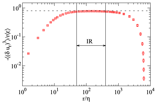
Figure 2.7: Verification of the four-fifths law in a numerical simulation from [109], with $8192^{3}$ grid points, and $\mathrm{Re}_{\lambda}=1300$. The dashed horizontal line corresponds to the theoretical prediction of the 4/5 law, and deviations from this result are used to define the inertial range.

The four-fifths law reveals that the velocity difference PDF is skewed, and the skewness is directly proportional to the energy dissipation. A numerical verification of this law can be seen in Fig. 2.7.

Inspired by the second hypothesis of Kolmogorov, Eq. (2.17), a scaling transformation applied to Eq. (2.37) reveals the scaling exponent of Navier-Stokes is $h=1/3$. If there is only one such scaling exponent, this results in a single functional form to all structure functions:

$$S_{p}(\ell)=\left\langle\left(\delta\mathbf{u}_{\|}(r,\ell)\right)^{p}\right\rangle=C_{p}(\varepsilon\ell)^{p/3}\ .$$ (2.39)

The $C_{p}$ are constants that do not depend on the Reynolds number, since the infinite Reynolds limit has already been taken in the derivation of the four-fifths law. It was a further hypothesis of Kolmogorov that the constants $C_{p}$ are universal at small scales, independent of the geometry or the forcing, although later criticism, especially from Landau, was made against the universality hypothesis. Among the constants, only $C_{3}$ is universal, and its value is given by the four-fifths law as $C_{3}=-4/5\varepsilon$. The exponents $p/3$, though, are understood to be universal, but their scaling is not linear as predicted by Kolmogorov. The critiques against universality are addressed in Section 2.5.3 and the nonlinearity of the exponents, a sign of intermittency, is discussed in the Sections 2.7 and 2.8. Despite these objections, $C_{2}$ has been measured in different settings and its value has been observed to be constant, and equal to $2.0\pm 0.4$, in different flow conditions [210].

2.5.2 The Energy Spectrum and the 5/3 Law

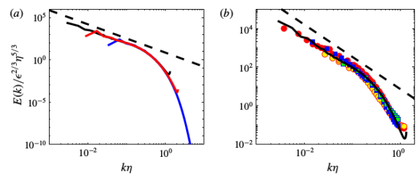
Figure 2.8: The kinetic energy spectrum is displayed at various values of Reynolds, dif- ferent forcing schemes and anisotropy conditions. In both figures, the black dotted line is the $k^{-5/3}$ scaling. In (a), results from numerical simulations are shown, while in (b), the black continuous line is from the Johns Hopkins Turbulence Database [217], at $\mathrm{Re}_{\lambda}=433$ [140], and the symbols are from several experiments, described in [47]. The figure was extracted from [53].

Another relevant observable for which K41 provides a prediction is the energy spectrum. It describes how energy is spread across different energy scales, and is obtained from the velocity two-point correlation function,

$$R_{ij}(\mathbf{r})=\langle u_{i}(\mathbf{x})u_{j}(\mathbf{x}+\mathbf{r})\rangle\ .$$ (2.40)

Its Fourier transform is defined as

$$\phi_{ij}(\mathbf{k})=\frac{1}{(2\pi)^{3}}\int R_{ij}(\mathbf{r})e^{-i\mathbf{k}\cdot\mathbf{r}}d\mathbf{r}\ ,$$ (2.41)

from which we obtain the energy spectrum $E(k)$ as an integral at fixed $k$ over all directions of the Fourier transformed correlation function:

$$E(k)=\oint\frac{1}{2}\phi_{ii}(\mathbf{k})dS(k)\ .$$ (2.42)

In this equation, $dS(k)$ is the surface integration element at a distance $k$ from the origin. Notice that $E(k)$ only depends on the absolute value of the wavenumber vector $\mathbf{k}$. Homogeneity and isotropy imply that all the information contained in the tensor $\phi_{ij}(\mathbf{k})$ can be described by the scalar $E(k)$ [186].

In the inertial range, since there is no characteristic length scale which can be formed only from $\varepsilon$, Kolmogorov argued that the transfer of energy can only be self-similar. This means the energy spectrum displays an algebraic dependence with the scale $k$, and this algebraic exponent can be found from dimensional analysis. Given that the kinetic energy dissipation is dimensionally equivalent to

$$[\varepsilon]=[dU/dt]=U^{2}/T=U^{3}/L=U^{3}\kappa\ ,$$ (2.43)

and the dimension of the energy spectrum is

$$[E(k)]=[\phi_{ii}dS(k)]=U^{2}\kappa^{-3}\kappa^{2}=U^{2}\kappa^{-1}\ ,$$ (2.44)

we obtain that a self-similar energy spectrum has the functional form:

$$E(k)=C_{K}\varepsilon^{2/3}k^{-5/3}\ ,$$ (2.45)

where $C_{K}$ is argued to be a universal constant called the Kolmogorov constant. Its value is approximately 1.5 [210].

In the dissipation range, there is a natural length scale provided viscosity, which hinders the algebraic behavior. Instead, the energy spectrum decays exponentially in this range. The first experimental results to show an agreement with the $5/3$ exponents were communicated in [94]. Despite the agreement, in the same year Kolmogorov proposed a refinement of the 1941 theory, which will be discussed in the next section. More recent measurements, both in DNS and in experiments, can be seen in Fig. 2.8, corroborating the predicted exponent. One can also see a spiked behavior at small wavenumbers, that corresponds to the forcing scale, where the energy input is concentrated, and a fast exponential decay at small spatial scales (large $k$).

2.5.3 The Critiques of Landau

Soon after the publication of the works of 1941, L. D. Landau expressed critiques regarding the hypothesis of universality. He argued that fluctuations could spoil universality, which was assumed for the constants $C_{p}$ and the exponents, in Eq. (2.39). These comments were made at a meeting in Kazan in 1942 and in a footnote in the first edition of his textbook in fluid mechanics, published in 1944 [78].

Landau devised an argument to show that, in a flow with more than one length scale present (for instance, if the grid generating turbulence has varying grid spacings), then there are local variations of the kinetic energy dissipation such that it is not possible to satisfy Eq. (2.39) both locally and globally for this flow (the only case in which this is possible is $p=3$). This version of the argument in terms of a flow with multiple length scales is presented in [78].

As a consequence, whatever is the mechanism used to generate local variations in $\varepsilon$, universality as proposed in Eq. (2.39) cannot be true. But fluctuations in the energy dissipation occur naturally, and they are quite strong in fully developed turbulence, even without any external mechanism to enhance space variations, such as a non-uniform grid.

The comments of Landau were brief, and some of them are known only through recounts in conference proceedings, hence they are still object of study as to their precise meaning, but substantial credit is given to them in [125], the extension of the 1941 theory which takes fluctuations into account.

2.6 Onsager’s Conjecture

A deeper connection between the solutions of the Euler and Navier-Stokes equations (at vanishing viscosity) is subject of a discussion originally stated in [171]. This discussion concerns the properties of weak solutions of the Euler equation.

Weak solutions are functions for which all derivatives may not exist, but which are still considered solutions of the respective differential equation. In contrast to them, standard solutions are also called strong solutions. This formulation was first developed in [138], where it was demonstrated that the Navier-Stokes equations possess weak solutions on the whole space, $\mathbb{R}^{d}$, with $d\geq 2$. In [103] this demonstration was expanded to limited domains. For other systems of differential equations, weak solutions are often an intermediate step to a general proof of regularity in the strong solutions, but this path has not been completed for the equations of fluid dynamics, either viscous or inviscid.

For the Navier-Stokes equations, Eq. (2.9), the formal definition of weak solutions are fields $p(\mathbf{r},t)$ and $\mathbf{u}(\mathbf{r},t)$ that satisfy the following equations [23]:

$$\begin{split}&\int_{\mathbb{R}^{3}\times\mathbb{R}}\Big{(}u_{i}\partial_{t}+u_{i}u_{j}\partial_{j}+\nu u_{i}\partial^{2}+p\partial_{i}+f_{i}\Big{)}\phi_{i}\ d\mathbf{r}\ dt=0\ ,\\ &\int_{\mathbb{R}^{3}\times\mathbb{R}}u_{i}\partial_{i}\psi\ d\mathbf{r}\ dt=0\ ,\end{split}$$ (2.46)

where $\bm{\phi}(\mathbf{r},t)$ and $\psi(\mathbf{r},t)$ are smooth functions of compact support, with the further constraint of $\partial_{i}\phi_{i}=0$. A similar definition, without the viscous term, holds for the weak solutions of the Euler equation.

Onsager, then, noticed that, while the Euler equation is a conservative system, its weak solutions, which may display rough and irregular behavior, need not conserve energy. That is, consider a weak solution of the Euler equation satisfying

$$\left|\mathbf{u}(\mathbf{r},t)-\mathbf{u}(\mathbf{r}^{\prime},t)\right|\leq C\left|\mathbf{r}-\mathbf{r}^{\prime}\right|^{\theta}$$ (2.47)

everywhere, where $C$ is independent of $\mathbf{r},\mathbf{r}^{\prime}$ and $t$. This condition is called Hölder continuity with an exponent $\theta>0$, which measures the roughness of the velocity field. If $\theta\geq 1$, the velocity field is differentiable, whereas if $\theta<1$, it is a continuous, but nowhere differentiable function, similar to ideal Brownian paths.

Onsager’s conjecture, regarding the weak solution $\mathbf{u}(\mathbf{r},t)$, states that:

1. If $\theta>1/3$, then this solution conserves energy;

2. If $\theta\leq 1/3$, there exist weak solutions that do not conserve energy.

The first part was proved in [42]. For the second part, dissipative solutions were first built by [198, 205], and a proof for the open interval $\theta<1/3$ was exhibited in [106] for $d\geq 3$, building upon an argument from [45]. Still, the proof for the case $\theta=1/3$ remains open.

The connection between the value $1/3$ in this conjecture and the value for the scaling exponent of the velocity field in Kolmogorov’s theory is seen immediately, but this fact was only explaned in [54]. In this article, it is demonstrated that the term responsible for dissipation in the weak solutions of the Euler equation is similar to the inertial transport term in the Navier-Stokes equation, $\mathcal{I}_{\ell}(\bm{u})$, Eq. (2.36). For this reason, the phenomenon of dissipative solutions in the Euler equations was called inertial dissipation, first described by Onsager:

It is of some interest to note that in principle, turbulent dissipation as described could take place just as readily wihout the final assistance by viscosity. In the absence of viscosity, the standard proof of the conservation of energy does not apply, because the velocity field does not remain differentiable! [171]

For this reason, it is also hypothesized that weak solutions of the Navier-Stokes equations at vanishing viscosity are equivalent to dissipative weak solutions of the Euler equation [65]. For a deeper discussion on this topic, the reader is referred to [46, 214] and references therein.

2.7 The Theory of 1962 and Intermittency

In 1962, the first experimental evidences of the success of K41 were still appearing, with new measurement techniques being developed. Nevertheless, there was already theoretical controversy on the limitations of this theory, such as the critiques of K41 by Landau. The role of fluctuations can be seen as crucial in these critiques. In this same year, Kolmogorov and Alexander Obukhov, a student of Kolmogorov, proposed an extension of the K41 theory, which accounts for large fluctuations, but which preserved universality at the small scales from K41. This theory is commonly called K62.

Among the phenomena considered in K62, there are deviations from the self-similar exponents of Eq. (2.39). Instead of linear exponents, scaling behavior with arbitrary exponents $\zeta_{p}$ is expected in the inertial range:

$$S_{p}(\ell)=\left\langle\left(\delta\mathbf{u}_{\|}(r,\ell)\right)^{p}\right\rangle=C_{p}(\varepsilon\ell)^{\zeta_{p}}\ .$$ (2.48)

Strong evidence of this discrepancy was only reported much later, in [4], and has been reinforced ever since. Several models have been proposed since 1962 to explain such deviations from the self-similar exponents, beginning with K62, but such models are still phenomenological and it is still difficult to answer precisely which of them describes the data the most accurately.

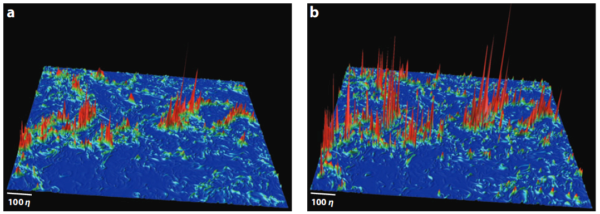
Figure 2.9: This figure, from the large scale numerical simulations of [107], shows strong spatial fluctuations in energy dissipation (a) and in enstrophy (b),

An observation from numerical simulations that strengthens the need for a statistical description of fluctuations can be seen in Fig. 2.9, where the values of kinetic energy dissipation and enstrophy are displayed, in a single instant, for a cross-section of a three-dimensional flow. These observables exhibit fluctuations which are very intense, in marked contrast with Gaussian noise, which would be evenly spread and of almost uniform intensity. Instead, there are turbulent spots where very large fluctuations can be observed.

This phenomenom is called intermittency. Intermittent fields display scale-dependent fluctuations, in which intense bursts are observed in small intervals (in space or time). A velocity field which displays such strong fluctuations, thus, cannot be accurately described by its mean value, requiring an understanding of its higher order statistics.

But measuring intermittent fluctuations and the structure function exponents from Eq. (2.48) is a challenge, because capturing large fluctuations requires very long time series, whether in numerical simulations or in experiments.

To take fluctuations into account, a new theory was developed in [124, 125, 169]. Its main hypothesis is that, instead of using the global mean energy dissipation, $\varepsilon$, its local scale averaged value should be considered. The kinetic energy dissipation averaged over a scale $\ell$ is

$$\varepsilon_{\ell}(\bm{x},t)=\frac{3}{4\pi\ell^{3}}\int_{\mathcal{B}_{\ell}(\mathbf{x})}\varepsilon(\bm{x+r},t)\ d\bm{r}\ ,$$ (2.49)

in which $\varepsilon$ is integrated over a ball $\mathcal{B}_{\ell}(\mathbf{x})$ of radius $\ell$ and center $\mathbf{x}$. This hypothesis was called local universality by Kolmogorov and Obukhov, and under this assumption, all statistical properties measured at scale $\ell$ in the inertial range, can only depend on $\varepsilon_{\ell}$, instead of the global quantity $\varepsilon$.

This addresses the critique of Landau: Universal scaling exponents, universal constants $C_{p}$ and non-homogeneities in the energy dissipation field cannot coexist under the linear scaling defined by Eq. (2.39), and not even for the nonlinear scaling of Eq. (2.48), for the reasons laid out in Sec. 2.5.3. Instead, if the scaling of the structure functions (or any other observable) at some scale $\ell$ is defined in terms of the local energy dissipation, as

$$S_{p}(\ell)=C_{p}(L)(\varepsilon_{\ell}\ell)^{\zeta_{p}}\ ,$$ (2.50)

no such problem exists. The local universality hypothesis warrants the replacement of $\varepsilon$ with $\varepsilon_{\ell}$, and the constants $C_{p}(L)$ are no longer universal, instead depending on the large scale. In this manner, the universality of the scaling exponents and the non-homogeneities of the energy dissipation field are maintained.

Along with the local universality hypothesis, a conjecture for the statistics of the energy dissipation was also made. It was established that $\varepsilon_{\ell}$ displays log-normal fluctuations, specified by

$$\begin{split}\langle\varepsilon_{\ell}\rangle&=\varepsilon\ ,\\ \mathrm{Var}[\ln\varepsilon_{\ell}]&=C-\mu\ln(\ell/L)\ .\end{split}$$ (2.51)

In this equation, $C$ is a non-universal constant that depends on the large scales and $\mu$ is a universal constant, called the intermittency parameter, which defines the strength of fluctuations. The higher its value, more intense is intermittency. Another element which is present in these equations is the integral length $L$. It is responsible for breaking the self-similar behavior (scale invariance).

The hypothesis of lognormal fluctuations can be justified with the Richardson cascade picture, in which the energy is transferred locally from a scale $\ell$ to a scale $a\ell$, with $a\leq 1$, in a self-similar way. The ratio between the energy dissipation at two nearby scales, $\varepsilon_{\ell}/\varepsilon_{a\ell}$, can be thought of as a random variable, its probability distribution depending only on the scale ratio $a$. Then, the whole cascade can be described as the product of several random factors which only depend on the same ratio, as

$$\frac{\varepsilon_{L}}{\varepsilon_{a^{N}L}}=\frac{\varepsilon_{L}}{\varepsilon_{aL}}\frac{\varepsilon_{aL}}{\varepsilon_{a^{2}L}}\cdots\frac{\varepsilon_{a^{N-2}L}}{\varepsilon_{a^{N-1}L}}\frac{\varepsilon_{a^{N-1}L}}{\varepsilon_{a^{N}L}}\ ,$$ (2.52)

for any $\ell=a^{N}L$. From this expression, $\ln\varepsilon_{\ell}$ is the sum of several variables with identical distributions of finite variance. If the ratios $\varepsilon_{a^{n}L}/\varepsilon_{a^{n+1}L}$ can be considered independent, then, as $N$ approaches infinity, the probability distribution of $\ln\varepsilon_{\ell}$ approaches a normal distribution, from the Central Limit Theorem. The probability distribution of $\varepsilon_{\ell}$ is correspondingly a lognormal.

The exponents $\zeta_{p}$ can be calculated from the distribution for the scale averaged energy dissipation. If the probability distribution of $\varepsilon$ is a lognormal with mean and variance given by Eq. (2.51), then any moment of $\varepsilon_{\ell}$ is given by

$$\langle\varepsilon_{\ell}^{p}\rangle\sim\varepsilon^{p}e^{-p(1-p)C/2}\left(\frac{\ell}{L}\right)^{\mu p(1-p)}.$$ (2.53)

Then, using the local universality hypothesis, it is observed that velocity fluctuations, in the inertial range and at scale $\ell$, only depend on the energy dissipation at this scale, $\varepsilon_{\ell}$, and on the scale itself. This means that $\delta u_{\ell}$ has the same scaling behavior as $(\ell\varepsilon_{\ell})^{1/3}$, from which the scaling of the structure functions is obtained:

$$\langle\left(\delta u_{\ell}\right)^{p}\rangle\sim\langle\left(\ell\varepsilon_{\ell}\right)^{p/3}\rangle\propto(\ell\varepsilon)^{p/3}\left(\frac{\ell}{L}\right)^{\mu(1-p/3)p/3}\ .$$ (2.54)

The anomalous exponents are calculated directly from this expression:

$$\zeta_{p}=\frac{p}{3}\left(1+\mu\left(1-\frac{p}{3}\right)\right)\ .$$ (2.55)

Several evidences for deviations from linear (self-similar) behavior have been reported. For numerical and experimental results, the reader is referred to [107, 20, 207, 109, 188].

The 1962 model is a rich and useful framework for dealing with large fluctuations. It is known that some properties of the exponents in Eq. (2.55) at high orders conflict with mathematical properties expected in general for them [78]. For this reason, more general models for fluctuations in turbulence have been proposed, which are discussed in the next section.

2.8 The Multifractal Model

The self-similar theory of 1941 is marked by a single scaling exponent, $h=1/3$. Yet, scale invariance is broken by the intermittent fluctuations, as can be seen in the K62 model. Another proposal which employs the language of scale invariance and includes fluctuations is called multifractality. A random velocity field with a single scaling exponent is also called a fractal, in general, because this scaling exponent is in direct correspondence with the fractal dimension of the random field. The multifractal approach, instead, states that a range of scaling exponents is possible, corresponding to a field with multiple fractal dimensions simultaneously.

This approach began in [143], where lognormal fluctuations of the energy dissipation are already treated under a multifractal view. Further developments were carried out in [79, 151, 152].

In the multifractal approach, it is supposed that there is a set $F\in\mathbb{R}^{3}$ of fractal dimension $D_{F}<3$ where energy dissipation events and intense fluctuations concentrate. The complement of this region is made of regular velocity fields, which can be linearized. In this region, the scaling exponent of the velocity field is $h\geq 1$, such that all velocity gradients remain small in this region. The set $F$ is a multifractal if it is a superposition of subsets $\mathcal{S}_{h}$, such that the velocity field scales with an exponent in the range $[h,h+dh]$ inside $\mathcal{S}_{h}$.

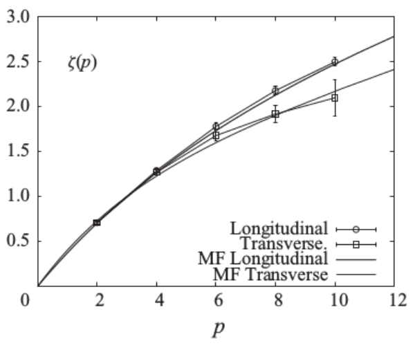
Figure 2.10: Structure functions from the numerical simulations of [20] display clear deviations from the linear prediction of K41. But exponents of order larger than eight are still hard to measure with precision due to the enourmous amount of data that is needed to capture large fluctuations.

In this context, the probability of sampling a singularity exponent close to $h$ is proportional to the size of the corresponding set $\mathcal{S}_{h}$, which is measured by the fractal dimension $D(h)$. This probability, then, is

$$\mathcal{P}_{\ell}(h)dh=\left(\frac{\ell}{L}\right)^{3-D(h)}\rho(h)dh\ .$$ (2.56)

The function $\rho(h)$ describes the distribution of values of $h$ in this velocity field, irrespective of the scale, it is thus a smooth function of $h$, independent of $\ell$. Then, the structure functions are given by

$$\int\left(\delta\mathbf{u}_{\|}(\bm{r},\ell)\right)^{p}\mathcal{P}_{\ell}(h)dh\sim\int\left(\ell\varepsilon_{\ell}\right)^{hp}\left(\frac{\ell}{L}\right)^{3-D(h)}\rho(h)dh\ .$$ (2.57)

Using a saddle-point aproximation for the structure functions, the structure function exponents are obtained as

$$\zeta_{p}=\underset{h}{\mbox{min}}[hp+3-D(h)]\ .$$ (2.58)

Direct measures of the structure functions from numerical simulations can be seen in Fig. 2.10. Deviations from the linear exponents of K41 are clearly seen.

The multifractal model is a general framework for anomalous scaling, but it does not provide a quantitative prediction for the exponents, which depend on an explicit $D(h)$ function. But relationships between exponents of different observables which can be predicted from the theory, and be used to test it. For instance, scaling exponents for the energy dissipation [143] or the velocity gradient [164] can be obtained as Legendre transforms of the $D(h)$ function, hence these exponents must be connected to those calculated in Eq. (2.58).

The former sections have demonstrated the relevance of fluctuations and probabilities in turbulence. The next chapter discusses techniques of stochastic calculus and statistical mechanics which are used in the works developed in this dissertation.

Chapter 3 Brief Review of Stochastic Methods

In 1827, the famous botanist Robert Brown observed that pollen immersed in water followed a strange jiggling motion, reported in [29]. Interested in investigating if this effect was a manifestation of life, he repeated the experiment with other suspensions of fine particles: Glass, minerals, and even a fragment of the sphinx. In all of these situations, the same jiggling motion was observed, thus ruling out any organic origin [85].

The origin of this mysterious motion was only resolved in 1905 by Albert Einstein, who also introduced the probabilistic description of physical phenomena in his solution [58]. This theory relied on the molecular nature of matter and the random motion of its molecules, agitated by thermal fluctuations. He predicted that the mean square displacement of a suspended particle would be

$$\langle x^{2}\rangle=2Dt\ .$$ (3.1)

Furthermore, the suspended particle is in thermal equilibrium, thus its kinetic energy is given by the equipartition law, which sets the value of the constant $D$ to

$$D=\frac{k_{B}T}{6\pi\mu a}\ .$$ (3.2)

In this equation, $k_{B}$ is the Boltzmann constant and $\mu$ is the dynamic viscosity of the fluid, it arises because of the Stokes drag in the suspended particle, assumed spherical of diameter $a$. Also, $\langle\ \bm{\cdot}\ \rangle$ represents an expectation value, calculated with respect to some probability distribution function.

With the theoretical framework developed by Einstein, the experimental physicist Jean Perrin was able to verify such random motion and calculate Avogadro’s constant, obtaining the surprisingly accurate value of $6.4\times 10^{23}\ \mathrm{mol}^{-1}$ [166]. This value was in close agreement with known results of the time, including other independent measures from Perrin, using several different experimental techniques. At the time, these experiments were seen as strong evidence of the existence of atoms and molecules and Perrin was awarded the Nobel Prize in Physics of 1926 “for his work on the discontinuous structure of matter” [2].

A few years after Einstein, the French physicist Paul Langevin was able to arrive at the same conclusions by proposing an equation of motion for the suspended particle [133]:

$$m\frac{d^{2}x}{dt^{2}}=-6\pi\mu a\frac{dx}{dt}+\eta_{t}\ .$$ (3.3)

In this equation, it is supposed that the particle of mass $m$ is subject to viscous drag (Stokes drag) by the medium and to a random external force $\eta_{t}$, which represents the incessant impact of the molecules of the liquid on the particle. He further assumed that this force would be positive and negative with equal probabilities. Eq. (3.3) was the first example of a stochastic differential equation used in physics, and from it the mean square displacement law can be derived as well, with the same constant $D$ that Einstein had obtained.

Earlier equivalent models for random motion were developed in the study of time series [218] and in stock markets [11], although they remained unacknowledged for a long time (see [113] for a historical review).

The random description of Brownian motion inspired the mathematicians Norbert Wiener, Raymond Paley and Antoni Zygmund to develop a rigorous mathematical explanation for the theory of Einstein. The construction which obeys Eq. (3.1) was demonstrated in 1923 and is called the Wiener process, or Wiener measure, which is informally treated as a synonym for Brownian motion. The Wiener process is the continuous-time stochastic process, $W_{t}$, which observes the following properties:

1. $W_{0}=0$;

2. $W$ has independent increments;

3. $W$ has Gaussian increments: $W_{t+s}-W_{t}$ is distributed with mean $0$ and variance $s$. This is represented by $W_{t+s}-W_{t}\overset{d}{=}\mathcal{N}(0,s)$;

4. $W$ has continuous paths. This means $W_{t}$ is almost surely continuous in $t$.

As before, the symbol $\overset{d}{=}$ means equality in distribution. Due to its simple properties, the Wiener process is used as the basis for numerous other stochastic processes and in applications to real systems.

The mathematical grounding for the theory of stochastic differential equations such as Eq. (3.3), though, was only developed years later by the Japanese mathematician Kiyosi Itô [108]. To make mathematical sense of such an equation, he developed the concept of the Itô stochastic integral, defined as the limit

$$\int_{t_{0}}^{t}G(t^{\prime})dW_{t^{\prime}}=\lim_{n\to\infty}\left[\sum_{i=i}^{n}G(t_{i-1})(W_{t_{i}}-W_{t_{i-1}})\right]\ .$$ (3.4)

Itô demonstrated that this integral converges in probability to a well defined random variable.

A well known figure who was also paramount to the theory of probability and stochastic processes was Andrey Kolmogorov, who established the axioms of probability theory and developed a theory for Markov processes. His work on Markov processes, which elicited the role of the drift and diffusion coefficients, inspired Itô in building a theory of stochastic calculus. His most famous contribution is discussed in the next section.

3.1 Itô’s Lemma

A generalized Langevin equation is usually written in mathematical notation as

$$du=b[u]dt+g[u]dW_{t}\ ,$$ (3.5)

where the Wiener process is the driving random contribution. The velocity $u$ is a vector in $\mathbb{R}^{d}$, $b[u]$ is a functional called the drift coefficient and $g[u]$ is the diffusion coefficient. This equation is similar to the one proposed by Langevin, and is often written in the physics literature as

$$\dot{u}=b[u]+g[u]\eta_{t}\ ,$$ (3.6)

where $\eta_{t}$ is called Gaussian white noise. Such noise source is equivalent to a time-derivative of the Wiener process, or, formally, its Radon-Nikodym derivative. Gaussian white noise can be characterized entirely by its mean and its two-point correlation function:

$$\begin{split}&\langle\eta(t)\rangle=0\ ,\\ &\langle\eta(t)\eta(t^{\prime})\rangle=\delta(t-t^{\prime})\ .\end{split}$$ (3.7)

One of the main results in the theory of stochastic processes, fundamental to the mathematical manipulation of equations such as Eq.  (3.6) is called Itô’s lemma. It is the formula for a change of variables in stochastic processes, hence it is an expression analogous to the chain rule of standard calculus. In the formula for the stochastic integral, Eq. (3.4), it can be seen that the prescription for a derivative has to be carefully specified. One of the consequences of this is that the formulation of the chain rule depends on the exact prescription. The Itô prescription for the derivative is the following:

$$\frac{du}{dt}=\lim_{\epsilon\to 0}\frac{u(t+\epsilon)-u(t)}{\epsilon}\ .$$ (3.8)

If $u$ is governed by Eq. (3.5), the stochastic differential equation which $f(u)$ obeys can be found using the Itô prescription:

$$\begin{split}\frac{df}{dt}&=\lim_{\epsilon\to 0}\frac{f(u(t+\epsilon))-f(u(t))}{\epsilon}\\ &=\lim_{\epsilon\to 0}\frac{f(u(t)+\epsilon\dot{u}(t)+\ldots)-f(u(t))}{\epsilon}\ .\end{split}$$ (3.9)

Then, $f$ can be expanded to second order in a Taylor series,

$$\begin{split}\frac{df}{dt}&\approx\lim_{\epsilon\to 0}\frac{1}{\epsilon}\left[f(u(t))+\epsilon\dot{u}(t)\frac{\partial f}{\partial u}+\frac{1}{2}\epsilon^{2}\dot{u}(t)^{2}\frac{\partial^{2}f}{\partial u^{2}}+\ldots-f(u(t))\right]\\ &\simeq\lim_{\epsilon\to 0}\left[\dot{u}(t)\frac{\partial f}{\partial u}+\frac{1}{2}\epsilon\dot{u}(t)^{2}\frac{\partial^{2}f}{\partial u^{2}}+O(\epsilon^{2})\right]\ .\end{split}$$ (3.10)

With $\dot{u}^{2}=b[u]^{2}+g[u]^{2}\eta_{t}^{2}+2b[u]g[u]\eta_{t}$ and $\eta_{t}^{2}=O(1/\epsilon)$, the expression for Itô’s lemma can be found:

$$\frac{df}{dt}=\dot{u}\frac{\partial f}{\partial u}+\frac{g[u]^{2}}{2}\frac{\partial^{2}f}{\partial u^{2}}\ .$$ (3.11)

In the differential formulation, this is written as

$$df=\left(b[u]\frac{\partial f}{\partial u}+\frac{g[u]^{2}}{2}\frac{\partial^{2}f}{\partial u^{2}}\right)dt+g[u]\frac{\partial f}{\partial u}dW_{t}\ .$$ (3.12)

The symbol $O(\ \bm{\cdot}\ )$ is used for asymptotic big-O notation.

A brief explanation of $\eta_{t}^{2}=O(1/\epsilon)$ is worthy of notice. From the properties of the Wiener process, it can be seen that $|W_{t+\epsilon}-W_{t}|$ is a term of the order of $\sqrt{\epsilon}$. Consequently, terms of second order in $|W_{t+\epsilon}-W_{t}|$ cannot be ignored, since they produce a first order contribution in $\epsilon$. The order of magnitude of $\eta_{t}$ can be found from its defining properties, Eq. (3.7) or from the knowledge that it is a time derivative of $dW_{t}$, resulting in $\eta_{t}^{2}=O(1/\epsilon)$. All of these statements can be proven, and the reader is referred to [85, sec.4.2.5] or [187, sec.2.5] on this topic. The former reference is more accessible to physicists in general, while the latter proof is more mathematically rigorous.

An alternative to the Itô prescription for the derivative is the Stratonovich one, given by

$$\frac{du}{dt}=\lim_{\epsilon\to 0}\frac{u(t+\epsilon/2)-u(t-\epsilon/2)}{\epsilon}\ .$$ (3.13)

An argument equivalent to the previous one, for the Itô prescription, produces the respective chain rule under the Stratonovich prescription, which is equal to the chain rule in standard calculus,

$$\frac{df}{dt}=\dot{u}\frac{\partial f}{\partial u}\ .$$ (3.14)

The standard chain rule naively seems to favor the use of the Stratonovich interpretation, but the differences in calculation go beyond this point. Eq. (3.6) leaves the interpretation ambiguous and the issue of which interpretation should be used in a physical problem depends on the details of the question, such as the source of noise.

Consider the case in which the variance of the noise $\eta_{t}$ is a known function with a finite correlation time $\epsilon$, instead of Gaussian white noise, which has a singular variance. It has been demonstrated that, in the limit $\epsilon\to 0$, the equation obtained is given in the Stratonovich prescription [156]. This is usually the case in situations of external noise: When a random force is added to an otherwise deterministic system. In these situations, $b[u]$ provides the deterministic dynamics of the system and the statistical properties of the noise can be studied independently.

In contrast, in systems where noise is intrinsic (or internal), it is harder to distinguish the drift and diffusion terms. This is the case of chaotic systems such as turbulence, where noise is unavoidable, as discussed in Sec. 2.3. In many such cases, the Itô prescription is the more appropriate interpretation because of its non-anticipating nature: The Itô prescription only requires knowledge of times up to $t$ to calculate derivatives and integrals at time $t$, while the Stratonovich interpretation requires knowledge of the future of $t$. This feature makes mathematical demonstrations much harder in the Stratonovich interpretation and favor the Itô view, which is employed in all stochastic differential equations in this dissertation.

Nevertheless, an SDE in the Stratonovich interpretation can be translated to an equivalent equation in the Ito interpretation, producing the same physical consequences (for instance, the same probability distribution function). A Stratonovich SDE is usually written as

$$du=b[u]dt+g[u]\circ dW_{t}\ ,$$ (3.15)

where the symbol $\circ$ indicates the use of the Stratonovich rule. This is equivalent to the following Itô SDE:

$$du=\left(b[u]+\frac{1}{2}\frac{\partial g[u]}{\partial u}g[u]\right)dt+g[u]dW_{t}\ .$$ (3.16)

A proof of this statement can be found in [62, sec.6.5.6].

The differences between prescriptions were settled in the discussions of [224, 225], and recently reviewed in [144].

At the same time, studying quantum mechanics, physicists developed another method to deal with the inherent fluctuations of quantum phenomena, namely the Feynman integral, or functional formalism. In the next section, the connections between the functional formalism and stochastic differential equations are developed.

3.2 The Functional Formalism

The theoretical framework of functional methods were first translated from quantum fields to the equilibrium statistical mechanics of systems near phase transitions. In this regime, the correlation length of these systems diverges, which makes the microscopic details irrelevant, and they can be described by a continuous limit, that is, a field theory [240, 3, 162].

Similarly to critical systems, turbulence is a phenomenom involving several length scales which displays universal behavior at small scales as well. The relation between these properties and the physics of statistical systems close to phase transitions was noticed quite early, and several researchers contributed to the understanding of both of these problems, turbulence, and critical systems, such as Landau and Onsager. But turbulence is already naturally described by continuous variables, the velocity and pressure, and no fine tuning is required to observe the scaling behavior of K41, unlike in phase transitions, where external parameters such as pressure and temperature have to be carefully chosen so the system displays critical behavior. The presence of exponents (that is, scaling behavior) has also drawn attention to the possibility of applying renormalization group methods, which were very successful in the study of critical systems to understand their scaling exponents and other universal quantities.

The use of functional methods in fluid dynamics began with [104], where a generating function for multi-point correlation functions of the velocity was investigated, without success. This approach spanned several derivative works [126, 139, 233, 215, 127], though they fail to account for intermittent fluctuations.

A change in paradigm was the development of field theoretical methods applied to classical stochastic systems. This was first done in [147], with canonical quantization techniques of quantum field theories. Later, they were extended to the language of functional integrals in [112, 51]. These developments are currently known as the Martin-Siggia-Rose-Janssen-de Dominicis (MSRJD) formalism, an established technique in the study of classical stochastic systems.

Other field theoretical approaches have been developed since the advent of the MSRJD formalism. As an example, methods in conformal field theory have been applied to turbulence in [183, 67, 69, 21] and applications of the non-perturbative renormalization group have been pursued in [149, 33]

The MSRJD approach is valid for any well posed stochastic differential equation (that is, given a smooth initial condition, it generates a unique solution for all times, for each realization of the noise). The following discussion, though, is limited to SDEs driven by additive Gaussian noise, but the method can be properly extended to other sources of noise through the careful evaluation of a Jacobian. Additive noise means that the diffusion term does not depend on the $u$ field, which is thus governed by the equation

$$\dot{u}=b[u]+g\eta\ .$$ (3.17)

The noise $\eta$ is Gaussian of zero mean and known two-point correlation, given by

$$\langle\eta(t)\eta(t^{\prime})\rangle=\chi(t-t^{\prime})\ .$$ (3.18)

The probability of any single realization of the noise is then given by the continuous limit of a multivariate normal distribution,

$$P[\eta]\propto\exp\left\{-\int dt\ \langle\eta,\chi^{-1}*\eta\rangle/2\right\}\ .$$ (3.19)

In the above expression, a convolution is represented by $*$ and its explicit formulation is

$$(f*g)(t)=\int_{-\infty}^{\infty}f(t-t^{\prime})g(t^{\prime})dt^{\prime}\ ,$$ (3.20)

and $\langle\ \bm{\cdot}\ ,\ \bm{\cdot}\ \rangle$ represents a suitable inner product, which depends on the dimensionality of the $u$ field.

This probability is the basis for calculating the expectation value of any observable $\mathcal{O}[u]$ which depends on the field $u$. For instance, some useful observables are $\mathcal{O}[u]=e^{i\lambda u(t)}$ and $\mathcal{O}[u]=u(t_{a})u(t_{b})$. The expectation value of the former is called the characteristic function, which is a Fourier transform of the probability distribution function, while the expectation value of the latter is the two-point correlation function.

Given any realization of the noise, $\eta$, the corresponding (unique) solution of the SPDE is represented by $u_{\eta}$ Then, the expectation value of any observable is calculated as

$$\langle\mathcal{O}[u]\rangle=\int D\eta\ \mathcal{O}[u_{\eta}]P[\eta]\ .$$ (3.21)

The functional integral is necessary because an integral is performed over all possible realizations of the noise, which is a time-dependent field. This can be understood by partitioning the time evolution of the system into small intervals, then this integral would be the limit of

$$\langle\mathcal{O}[u]\rangle=\lim_{n\to\infty}\int d\eta_{t_{1}}d\eta_{t_{2}}\cdots d\eta_{t_{n-1}}\ \mathcal{O}[u_{\eta}]P[\eta]\ .$$ (3.22)

This equation can be equivalently written with an extra functional integral over all possible $u$ fields:

$$\langle\mathcal{O}[u]\rangle=\int DuD\eta\ \mathcal{O}[u]\delta[u-u_{\eta}]P[\eta]\ .$$ (3.23)

$\delta[u]$ is a functional Dirac-delta, which filters the value of the integral over the $u$ field at each instant of time. Since $u_{\eta}$ is a solution of Eq. (3.17), a change of variables can be perfomed to replace it with the stochastic equation itself:

$$\langle\mathcal{O}[u]\rangle=\int DuD\eta\ \mathcal{J}\ \mathcal{O}[u]\delta[\dot{u}-b[u]-g\eta]P[\eta]\ .$$ (3.24)

There is a Jacobian which arises from the change of variables, $\mathcal{J}$, but it does not depend on $u$ for the case of additive noise (it is also important that Eq. (3.17) is interpreted with the Itô prescription). A proof of this can be found in [163]. In this case, the Jacobian is simply a normalization constant and can be neglected.

Rewriting the functional Dirac delta as a Fourier transform of a constant, an auxiliary field $p$ is introduced. Then, discarding all normalization constants, the desired expectation value can be written as

$$\langle\mathcal{O}[u]\rangle\propto\int DuD\eta Dp\ \mathcal{O}[u]\ e^{-i\int dt\ \langle p,u-b[u]-g\eta\rangle}e^{-\frac{1}{2}\int dt\langle\eta,\chi^{-1}*\eta\rangle}\ .$$ (3.25)

All terms involving the noise can be exactly integrated. Making the substitution $\eta\to\eta-i\chi*p$:

$$\int D\eta\ e^{-\frac{1}{2}\int dt\langle\eta,\chi^{-1}*\eta\rangle+ig\int dt\langle p,\eta\rangle}\xrightarrow[\eta\to\eta-i\chi*p]{}\int D\eta\ e^{-\frac{g^{2}}{2}\int dt\langle\eta,\chi^{-1}*\eta\rangle-\frac{1}{2}\int dt\langle p,\chi*p\rangle}\ .$$ (3.26)

On the right hand side of this expression, the last term under the integral does not depend on the noise, while the first is quadratic on $\eta$. The integral of this term is a Gaussian integral, which provides a constant contribution. Thus, the final form of the MSRJD functional is:

$$\langle\mathcal{O}[u]\rangle\propto\int DuDp\ \mathcal{O}[u]\ e^{-i\int dt\ \langle p,\dot{u}-b[u]\rangle}e^{-\frac{g^{2}}{2}\int dt\langle p,\chi*p\rangle}\ ,$$ (3.27)

from which any statistical observable can be calculated, in principle. It is worth mentioning, though, that technical difficulties on the exact evaluation of Eq. (3.27) are the standard, as it happens in any nonlinear field theory.

It is also common, in connection with statistical field theory, to name the (negative) argument of the exponential the MSRJD action:

$$S[u,p]=i\int dt\ \langle p,\dot{u}-b[u]\rangle+\frac{g^{2}}{2}\int dt\langle p,\chi*p\rangle\ .$$ (3.28)

This is the starting point for any application of the method, where a variety of field theoretical tools can be applied. It is important to remark that the above derivation is valid for Langevin equations with additive noise. In the case of multiplicative noise, the contribution of the Jacobian determinant must be carefully examined, and the choice of discretization is relevant for this. A discussion on multiplicative noise in functional methods can be found in [8] and a general discretization, which interpolates between the Itô and Stratonovich cases (the $\alpha$-discretization) is found in [111].

3.3 The Instanton Method

The difficulties in dealing with functional integrals such as Eq. (3.28) are notorious. The great success of quantum electrodynamics in making experimental predictions relies on the presence of a naturally perturbative parameter, the fine structure constant. Similarly, the first applications of the MSRJD formalism to fluid dynamics also relied on expansions around the zero field solution [76]. Nevertheless, there is no natural perturbative parameter in the problem of turbulence and intermittent fluctuations is one of its main ingredients. The standard perturbative expansion, developed around the “vacuum”, thus cannot account for these effects.

Another approach is the method of background field expansion. Instead of a perturbative expansion around the zero field, this method relied on the expansion around classical (or saddle-point) solutions of the action. In the context of disordered systems in solid state physics, the first applications of the background field method were done in [241, 131, 132]. In fluid dynamics, the background expansion was first perfomed for the Burgers equation, a one-dimensional version of Navier-Stokes, in [97]. In this setting, the authors studied the tails of the velocity gradient PDF. This problem has been only partially resolved and is further investigated in Chap. 5.

The background field expansion was originally developed in the context of Yang-Mills theory in [18]. The saddle-point solutions of the respective Euclidean field theory, which also display non-trivial topology, were called instantons. This name was a reference to solitons, waves localized in space, while the instantons are fast transitions between different ground states, hence they are solutions localized in time [197].

At the heart of the method is the realization that a functional integral reduces to the semi-classical limit in the presence of a small parameter. Then, the integral can be approximated by its saddle point approximation, using the solution that minimizes the action. In the literature of stochastic hydrodynamics, these solutions are called instantons as well, and represent the maximum likelihood realization of a specific event. The observed events are usually extreme fluctuations of intermittent observables, such as velocity gradients, vorticity, local energy dissipation, or circulation. This approach captures the leading behavior of the PDF of the desired observable, but it must be supplemented with fluctuations beyond the instanton to represent the true probability distribution.

For instance, consider the observable

$$\mathcal{O}[u]=\delta(F[u(x,t=0)]-a)\ .$$ (3.29)

This means that the event in question is the observable $F$ having the value $a$ at time $t=0$. The system is allowed to evolve for an infinite time, from $-\infty$ to $0$, to develop the value $F[u]=a$ at $t=0$. Large velocity gradients are one common instance of observable of interest, which is associated to $F[u]=u_{x}\delta(x)$.

In the MSRJD framework, the probability of such an event is

$$\begin{split}P(a)&=\langle\delta(F[u(x,t=0)]-a)\rangle\\ &=\int DuDp\ \frac{1}{2\pi}\int_{-\infty}^{\infty}d\lambda\ \mathcal{J}[u]\ e^{-S[u,p]}e^{-i\lambda(F[u]\delta(t)-a)}\ .\end{split}$$ (3.30)

In the limit of extreme fluctuations, $|a|\to\infty$, this integral can be estimated from its stationary contribution. As the $u$ and $p$ fields develop extreme values, the action $S[u,p]$ also grows, which justifies the saddle-point approach. This limit is also equivalent to $|\lambda|\to\infty$ or to $\chi(0)\to 0$, corresponding to large fluctuations and vanishing intensity of the external force, respectively. The instanton configuration corresponds to the most probable trajectory compatible with the observable. In the quantum mechanical analogue, this is the classical trajectory obtained with $\hbar\to 0$.

The functional derivative of the MSRJD action yields equations for the instanton fields, corresponding to the extremal points of the action functional:

$$\frac{\delta S}{\delta p}=i(\dot{u}-b[u])+\chi*p\ ,$$ (3.31)

$$\frac{\delta S}{\delta u}=-i\dot{p}-i(\nabla_{u}b[u])^{T}p\ .$$ (3.32)

The contributions from the Lagrange multiplier (the observable) provide an initial condition to the instanton fields, which satisfy the following equations:

$$\dot{u} =b[u]+i\chi*p\ ,$$ (3.33)

$$\dot{p} =-(\nabla_{u}b[u])^{T}p+i\lambda\nabla_{u}F[u]\delta(t)\ .$$ (3.34)

Integrating around $t=0$, the second equation can be used to obtain the initial condition for the $p$ field. It is assumed that $p(0^{+})=0$ for stability reasons, otherwise $p$ would grow without bounds and the action would diverge. Furthermore, the time evolution of the system is only considered for $t\leq 0$. The equations obtained for $p$ are:

$$\begin{split}\dot{p}&=-(\nabla_{u}b[u])^{T}p\ ,\\ p(0^{-})&=-i\lambda\nabla_{u}F[u(x,t=0)]\ .\end{split}$$ (3.35)

The instanton approach can likewise be developed in the language of large deviation theory, the mathematical framework that studies the asymptotic behavior of probability distributions [226]. The connection between the methods of statistical field theory and large deviation theory has been explored in [59, 220].

Nevertheless, the instanton is only the leading contribution to the probability distribution function of the observable. This approximation is more accurate in the limit of large fluctuations, but other effects have to be considered away from this regime. One possible approach is to consider perturbative fluctuations to the instanton field, with an expansion of the form

$$\begin{split}&u=u_{s}+\delta u\ ,\\ &p=p_{s}+\delta p\ ,\end{split}$$ (3.36)

where the subscript $s$ indicates the instanton (or saddle-point) fields and $\delta u$ and $\delta p$ are fluctuating fields. After this change of variables, the MSRJD action can be split into instanton and fluctuation contributions,

$$S[u,p]=S[u_{s},p_{s}]+\Delta S[u_{s},p_{s},\delta u,\delta p]\ .$$ (3.37)

In this equation, the first term is called the instanton action. Corrections of first order in the instanton fields do not play a role because the instanton solutions are extremal solutions of the action, by definition. Thus, the second term carries the contributions of quadratic and higher order in the fluctuation fields, as well as a possible dependence on the instantons themselves. A detailed treatment of fluctuations in two models of turbulence is going to be the subject of the next chapters.

The cumulant expansion is used in these particular cases, a standard method in statistical field theory which has been applied to classical stochastic systems since [134]. This is a perturbative method, hence its validity is limited to regimes in which the diagrammatic contributions in Eq. (3.37) are small relative to the instanton contribution, that is: $\Delta S[u_{s},p_{s},\delta u,\delta p]/S[u_{s},p_{s}]\ll 1$. This condition is met either for small fluctuation intensities ($g\ll 1$) or at large fluctuations of the observable being investigated.

Chapter 4 Instantons and Fluctuations in a Lagrangian Model of Turbulence

Intermittency has been measured in Galilean-invariant observables such as velocity differences and velocity gradients since [17]. Such observables have gained considerable interest in the last decades with the introduction of new experimental techniques to measure all nine components of the velocity gradient tensor, [230, 222, 237, 231, 232, 118]. These novel precise measurements inspired new attempts in the modeling of the velocity gradient dynamics [78, 38, 39], which offers a chance of studying the small scale fluctuations decoupled from the dynamics of large eddies, hence their recent theoretical and experimental interest.

The evolution of the Lagrangian velocity gradient $A_{ij}=\partial_{j}u_{i}$ can be obtained from a gradient of the Navier-Stokes equations ($\frac{\partial}{\partial x_{j}}(N.S.)_{i}$), resulting in

$$\frac{dA_{ij}}{dt}=-A_{ik}A_{kj}-\frac{\partial^{2}p}{\partial x_{i}\partial x_{j}}+\nu\frac{\partial^{2}A_{jj}}{\partial x_{k}\partial x_{k}}\ .$$ (4.1)

In this equation, $d/dt$ stands for the Lagrangian material derivative, $d/dt\equiv\partial/\partial t+u_{k}\partial/\partial x_{k}$. The Lagrangian framework describes the changes of the velocity gradient as it moves along the fluid particle trajectories in the flow, hence $A_{ij}(\mathbf{x},t)$ depends only on the initial position of the fluid particle $\mathbf{x}$, and evolves in time. Nevertheless, Eq. (4.1) is not closed in terms of the velocity gradient on a single trajectory $A_{ij}(\mathbf{x},t)$, because of the last two terms in the right hand side, respectively the pressure Hessian and the viscous term. These terms depend on neighboring Lagrangian trajectories as well. Furthermore, the incompressibility condition provides the equation

$$\nabla^{2}p=-A_{lk}A_{kl}\ ,$$ (4.2)

which is a highly nonlocal condition for the pressure field. Eq. (4.1) is usually rewritten in a form which isolates local and nonlocal contributions, as

$$\frac{dA_{ij}}{dt}=-\left(A_{ik}A_{kj}-\frac{1}{3}A_{mk}A_{km}\delta_{ij}\right)+H_{ij}^{P}+H_{ij}^{\nu}\ ,$$ (4.3)

where the pressure and viscous contribution are, respectively

$$H_{ij}^{p}=-\left(\frac{\partial^{2}p}{\partial x_{i}\partial x_{j}}-\frac{1}{3}\nabla^{2}p\delta_{ij}\right)\quad\text{ and }\quad H_{ij}^{\nu}=\nu\frac{\partial^{2}A_{ij}}{\partial x_{k}\partial x_{k}}\ .$$ (4.4)

The observation that Eq. (4.1) is unclosed has led to the development of several closure formulations, trying to simplify the equations and still capture the phenomena they describe. The simplest closed Lagrangian model is the Restricted Euler Equation, in which the nonlocal and anisotropic contributions $H_{ij}^{p}$ and $H_{ij}^{\nu}$ are ignored. This model was first considered in [137] and many of its properties were elicited in [227, 228].

Numerous other models, including linear damping, stochastic forcing and geometric effects have been developed since the Restricted Euler equation ([146, 89, 37, 114]). An extensive review is available in [150]. This chapter focuses on the Recent Fluid Deformation (RFD) approach, presented in [39].

The RFD model was recast in the Martin-Siggia-Rose-Janssen-de Dominicis (MSRJD) formulation in [160], where it was suggested that noise renormalization is the main physical mechanism to be considered to understand the onset of fat tails in the PDFs of velocity gradients, a point supported in [96]. But the approach of [160] relied on simplifying hypothesis which were not rigorously verified. The work which generated this chapter, [6], addresses these hypotheses.

4.1 The RFD Model

A natural stochastic extension to the velocity gradient dynamics (Eq. 4.1) is

$$\dot{{\mathbf{A}}}=V[{\mathbf{A}}]+g\mathbf{F}\ ,\$$ (4.5)

where $V[{\mathbf{A}}]$ is a nonlinear and nonlocal functional of ${\mathbf{A}}$, defined from Eq. (4.1). There is a random external force, $\mathbf{F}=\mathbf{F}(t)$, of null trace and entries given by a Gaussian stochastic process of zero mean and two-point correlation:

$$\langle F_{ij}(t)F_{kl}(t^{\prime})\rangle\equiv G_{ijkl}\delta(t-t^{\prime})\ ,\$$ (4.6)

where

$$G_{ijkl}=2\delta_{ik}\delta_{jl}-\frac{1}{2}\delta_{il}\delta_{jk}-\frac{1}{2}\delta_{ij}\delta_{kl}\ .$$ (4.7)

This is the most general fourth-order isotropic tensor consistent with the symmetries of Eq. (4.5) [186]. The stochastic force strength $g$ is proportional to the energy dissipation rate per unit mass, and can be seen as a perturbative coupling constant. The incompressibility condition, $\partial_{i}u_{i}=0$, is equivalent to $\mathrm{Tr}\ \mathbf{A}=0$.

It is interesting to notice that $\mathbf{A}$ and $\mathbf{F}$ only depend on time and not on space, thus making Eq. (4.5) a closed system. This is achieved through the modeling of the pressure Hessian and the viscous term of Eq. (4.1), which are replaced by local algebraic functions of the velocity gradient tensor. The closure for the RFD model is obtained from the assumption that velocity gradients are only correlated on short time scales. Hence, the nonlocal contributions can be assumed as isotropic at an arbitrary initial instant of the time evolution. With these assumptions, two time scale parameters are required in the model, $\tau$ and $T$, respectively corresponding to the dissipative and integral scales. These parameters generate an intermittent system corresponding to Lagrangian turbulence of Reynolds number $Re=f(g)(T/\tau)^{2}$, where $f(g)$ is some unknown (probably monotonic) analytical function of the coupling constant $g$.

Mathematically, these assumptions are expressed as the following approximation to $V[{\mathbf{A}}]$:

$$V({\mathbf{A}})=-{\mathbf{A}}^{2}+\frac{\mathrm{Tr}({\mathbf{A}}^{2})}{\mathrm{Tr}(\mathbf{C}^{-1})}\mathbf{C}^{-1}-\frac{\mathrm{Tr}(\mathbf{C}^{-1})}{3T}{\mathbf{A}}\ ,\$$ (4.8)

where $\mathbf{C}$ is the approximate Cauchy-Green tensor,

$$\mathbf{C}=\exp[\tau{\mathbf{A}}]\exp[\tau{\mathbf{A}}^{\mathrm{T}}]\mbox{,}$$ (4.9)

which governs the deformation in time of advected fluid blobs, within dissipative time scales.

Since only the ratio $\tau/T$ has physical significance in the model, the value $T=1$ can be used. Furthermore, in numerical simulations, it was observed that a perturbative expansion of the potential $V(\mathbf{A})$ up to $O(\tau^{2})$ is enough to capture its quantitative features [1, 160]. This expansion is given by

$$V({\mathbf{A}})=\sum_{p=1}^{4}V_{p}({\mathbf{A}})\ ,\$$ (4.10)

where each $V_{p}({\mathbf{A}})$ collects velocity gradient contributions of $O({\mathbf{A}}^{p})$:

$$\begin{split}V_{1}({\mathbf{A}})=&-{\mathbf{A}}\mbox{,}\\ V_{2}({\mathbf{A}})=&-{\mathbf{A}}^{2}+\frac{\text{1}}{3}\mathrm{Tr}({\mathbf{A}}^{2})\mbox{,}\\ V_{3}({\mathbf{A}})=&-\frac{\tau}{3}\left({\mathbf{A}}+{\mathbf{A}}^{\mathrm{T}}-\frac{2\text{1}}{3}\mathrm{Tr}({\mathbf{A}})\right)\mathrm{Tr}({\mathbf{A}}^{2})-\frac{\tau^{2}}{3}\mathrm{Tr}({\mathbf{A}}^{\mathrm{T}}{\mathbf{A}}){\mathbf{A}}-\frac{\tau^{2}}{3}\mathrm{Tr}({\mathbf{A}}^{2}){\mathbf{A}}\mbox{,}\\ V_{4}({\mathbf{A}})=&-\frac{\text{1}}{9}\tau^{2}\mathrm{Tr}({\mathbf{A}}^{\mathrm{T}}{\mathbf{A}})\mathrm{Tr}({\mathbf{A}}^{2})-\frac{\text{1}}{9}\tau^{2}[\mathrm{Tr}({\mathbf{A}}^{2})]^{2}+\frac{\tau^{2}}{3}{\mathbf{A}}^{\mathrm{T}}{\mathbf{A}}\ \mathrm{Tr}({\mathbf{A}}^{2})\\ &+\frac{\tau^{2}}{6}({\mathbf{A}}^{2}+{\mathbf{A}}^{2\mathrm{T}})\ \mathrm{Tr}({\mathbf{A}}^{2})\mbox{.}\end{split}$$ (4.11)

The RFD model is capable of reproducing several of the statistical features of the turbulent fluctuations of the velocity gradient tensor, observed in numerical simulations and experiments. Close to $g=1.0$, the domain of validity of the model is approximately given by the range $0.05<\tau<0.2$. Outside of this range, it was observed in [39], that the velocity gradient PDFs in the RFD model are strongly dissimilar from experimental and numerical results.

4.2 Path-Integral Formulation of Stochastic Lagrangian Models

The MSRJD formalism, as described in Chapter 3 is used to express the conditional probability density function of finding ${\mathbf{A}}={\mathbf{A}}_{1}$ at time $t=0$, provided that ${\mathbf{A}}={\mathbf{A}}_{0}$ at the initial time $t=-\beta$, as

$$\rho({\mathbf{A}}_{1}|{\mathbf{A}}_{0},\beta)\propto\int_{\Sigma}D[\hat{\mathbf{A}}]D[{\mathbf{A}}]\exp\left\{-S[\hat{\mathbf{A}},{\mathbf{A}}]\right\}\mbox{.}$$ (4.12)

In this equation: The auxiliary field is denoted by $\hat{\mathbf{A}}$. The boundary conditions for the path integral are represented by $\Sigma=\{{\mathbf{A}}(-\beta)={\mathbf{A}}_{0},\ {\mathbf{A}}(0)={\mathbf{A}}_{1}\}$. And the MSRJD action is

$$S[\hat{\mathbf{A}},{\mathbf{A}}]\equiv\int_{-\beta}^{0}dt\left\{i\mathrm{Tr}[\hat{\mathbf{A}}^{\mathrm{T}}(\dot{\mathbf{A}}-V({\mathbf{A}}))]+\frac{g^{2}}{2}G_{ijkl}\hat{A}_{ij}\hat{A}_{kl}\right\}\mbox{.}$$ (4.13)

The stationary state solutions of the RFD equations correspond to large asymptotic times, $\beta\rightarrow\infty$. Furthermore, it can be assumed that for such times the dependence on the initial condition ${\mathbf{A}}_{0}$ has vanished, making it possible to require periodic boundary conditions in the velocity gradient field,

$${\mathbf{A}}(0)={\mathbf{A}}(-\beta)\equiv\bar{\mathbf{A}}\ .$$ (4.14)

This approach was pursued in [160], leading to an analytical simplification in the saddle-point equations of the MSRJD action. The PDF for a stationary state configuration of the system is then reached as the limit

$$\rho(\bar{\mathbf{A}})=\lim_{\beta\rightarrow\infty}\rho(\bar{\mathbf{A}}|\bar{\mathbf{A}},\beta)\mbox{.}$$ (4.15)

As addressed in the general discussion on the MSRJD method, the principal features of the PDF in Eq. (4.15) are captured by the instanton configuration, the solution to the saddle point equations of the MSRJD action (Eq. (4.13)). This solution is called the instanton field, denoted by $\hat{\mathbf{A}}^{sp}$ and ${\mathbf{A}}^{sp}$, where $sp$ stands for “saddle point”. The PDF obtained solely from the instanton fields already captures nontrivial (non Gaussian) behavior induced by the nonlinearity and nonlocality of the Navier-Stokes equation, or an approximation such as the RFD equation. The instanton fields are the solutions of the Euler-Lagrange equations

$$\left.\frac{\delta S[\hat{\mathbf{A}},{\mathbf{A}}]}{\delta A_{ij}}\right|_{\begin{subarray}{c}\hat{\mathbf{A}}=\hat{\mathbf{A}}^{sp}\\ {\mathbf{A}}={\mathbf{A}}^{sp}\end{subarray}}\!\!\!\!\!\!=0\ \ \mbox{and}\ \ \left.\frac{\delta S[\hat{\mathbf{A}},{\mathbf{A}}]}{\delta\hat{A}_{ij}}\right|_{\begin{subarray}{c}\hat{\mathbf{A}}=\hat{\mathbf{A}}^{sp}\\ {\mathbf{A}}={\mathbf{A}}^{sp}\end{subarray}}\!\!\!\!\!\!=0\mbox{,}$$ (4.16)

with the periodic boundary condition ${\mathbf{A}}^{sp}(0)={\mathbf{A}}^{sp}(-\beta)=\bar{\mathbf{A}}$.

Besides the instanton solution, fluctuations around these configurations are relevant as well in the reproduction of the correct PDFs from the original model. To consider the effect of fluctuations, the velocity gradient fields in the MSRJD action are replaced as $\hat{\mathbf{A}}\rightarrow\hat{\mathbf{A}}^{sp}+\hat{\mathbf{A}}$ and ${\mathbf{A}}\rightarrow{\mathbf{A}}^{sp}+{\mathbf{A}}$, where $\hat{\mathbf{A}}$ and ${\mathbf{A}}$ on the right hand side of these transformations refer to the fluctuation contributions. Since the potential $V(\mathbf{A})$ has been approximated by a sum of polynomials in $\mathbf{A}$, the MSRJD action can be split in the form

$$S[\hat{\mathbf{A}},{\mathbf{A}}]\rightarrow S[\hat{\mathbf{A}},{\mathbf{A}}]=S_{sp}[\hat{\mathbf{A}}^{sp},{\mathbf{A}}^{sp}]+\Delta S[\hat{\mathbf{A}},{\mathbf{A}}]\ .$$ (4.17)

The above expression is exact: The first term, $S_{sp}[\hat{\mathbf{A}}^{sp},{\mathbf{A}}^{sp}]$ , holds the contributions to the MSRJD action that contain only the instanton fields, while all the additional terms that involve the fluctuations ${\mathbf{A}}$ and $\hat{\mathbf{A}}$ are included in $\Delta S[\hat{\mathbf{A}},{\mathbf{A}}]$. The saddle-point action $S_{sp}[\hat{\mathbf{A}}^{sp},{\mathbf{A}}^{sp}]$ is simply the MSRJD action, (4.13), evaluated on the instanton fields, $\hat{\mathbf{A}}^{sp}$ and ${\mathbf{A}}^{sp}$. From (4.12), (4.15), and (4.17), the vgPDF can be correspondingly rewritten as

$$\rho(\bar{\mathbf{A}})=\exp\left\{-S_{sp}[\hat{\mathbf{A}}^{sp},{\mathbf{A}}^{sp}]\right\}\int D[\hat{\mathbf{A}}]D[{\mathbf{A}}]\exp\left\{-\Delta S[\hat{\mathbf{A}},{\mathbf{A}}]\right\}\mbox{.}$$ (4.18)

The above path integral can be perturbatively computed following a standard procedure of statistical field theory, the cumulant expansion [3]. With this application in mind, the $\Delta S[\hat{\mathbf{A}},{\mathbf{A}}]$ term is exactly split as

$$\Delta S[\hat{\mathbf{A}},{\mathbf{A}}]=\Delta S_{0}[\hat{\mathbf{A}},{\mathbf{A}}]+\Delta S_{1}[\hat{\mathbf{A}},{\mathbf{A}}]\mbox{,}$$ (4.19)

where $\Delta S_{0}[\hat{\mathbf{A}},{\mathbf{A}}]$ contains only the quadratic contributions, whereas $\Delta S_{1}[\hat{\mathbf{A}},{\mathbf{A}}]$ holds all the self-interacting terms of the MSRJD action. Under this separation, the velocity gradient PDF is calculated as

$$\rho(\bar{\mathbf{A}})=\exp\left\{-S_{sp}[\hat{\mathbf{A}}^{sp},{\mathbf{A}}^{sp}]\right\}\left\langle\exp[-\Delta S_{1}]\right\rangle_{0},$$ (4.20)

where the expectation value $\left\langle\exp[-\Delta S_{1}]\right\rangle_{0}$ is computed with respect to the model defined by the quadratic action $\Delta S_{0}$. The PDF in Eq. (4.20) can be seen as

$$\rho(\bar{\mathbf{A}})\propto\exp\left\{-\Gamma[\hat{\mathbf{A}}^{sp},{\mathbf{A}}^{sp}]\right\},$$ (4.21)

where $\Gamma[\hat{\mathbf{A}}^{sp},\mathbf{A}^{sp}]$ is the effective action, taking into account the contributions from fluctuations around the instanton.

The cumulant expansion is a pragmatic way to evaluate the effective action from the statistical moments of $\Delta S_{1}$. Up to second order in $\Delta S_{1}$, the result of this expansion is

$$\begin{split}\Gamma[\hat{\mathbf{A}}^{sp},{\mathbf{A}}^{sp}]&=S_{sp}[\hat{\mathbf{A}}^{sp},{\mathbf{A}}^{sp}]+\langle\Delta S_{1}[\hat{\mathbf{A}}^{sp},{\mathbf{A}}^{sp}]\rangle_{0}\\ &-\frac{1}{2}\left(\langle\Delta S_{1}^{2}[\hat{\mathbf{A}}^{sp},{\mathbf{A}}^{sp}]\rangle_{0}-\langle\Delta S_{1}[\hat{\mathbf{A}}^{sp},{\mathbf{A}}^{sp}]\rangle_{0}^{2}\right)\mbox{.}\end{split}$$ (4.22)

A derivation of this formula is found in Appendix B. Each term in the cumulant expansion corresponds to a Feynman diagram with respect to the free theory $\Delta S_{0}$. These diagrams can be numerous, with a variety of relative weights, requiring a power counting procedure to single out the most relevant diagrams. This discussion is provided in the next section.

It should be emphasized that it is in general difficult to find exact solutions of the saddle-point Eqs. (4.16). This, however, should not be a matter of great concern, if one is able to find reasonable approximations for the instanton fields, since the substitution (4.17) and the second order cumulant expansion result (4.22) are always meaningful perturbative procedures in weak coupling regimes.

Provided that the Reynolds numbers are not too high, the exact instantons can be approximated by closed analytical expressions derived from the quadratic contributions to the MSRJD action. It is important to have in mind that such a simplification would not work to model the far PDF tails, essentially dependent on the exact nonlinear instantons (in cases where the PDF tails decay faster than a simple exponential).

4.3 Application to the RFD Model

In this section, the MSRJD formalism, discussed in the last section, is applied to the RFD model. The notation below follows the one introduced in Eq. (4.19). The quadratic action is given by

$$\Delta S_{0}[\hat{\mathbf{A}},{\mathbf{A}}]=\int_{-\beta}^{0}dt\left\{i\mathrm{Tr}[\hat{\mathbf{A}}^{\mathrm{T}}(\dot{\mathbf{A}}+{\mathbf{A}})+\frac{g^{2}}{2}G_{ijkl}\hat{A}_{ij}\hat{A}_{kl}\right\}\ ,$$ (4.23)

and the interaction term by

$$\begin{split}\Delta S_{1}[\hat{\mathbf{A}},{\mathbf{A}}]&=-i\sum_{p=2}^{4}\int_{-\beta}^{0}dt\ \mathrm{Tr}[(\hat{\mathbf{A}}^{sp})^{\mathrm{T}}(V_{p}({\mathbf{A}})+\Delta V_{p}({\mathbf{A}}))]\\ &+\mathrm{Tr}[\hat{\mathbf{A}}^{\mathrm{T}}V_{p}({\mathbf{A}}^{sp})]+\mathrm{Tr}[\hat{\mathbf{A}}^{\mathrm{T}}(V_{p}({\mathbf{A}})+\Delta V_{p}({\mathbf{A}}))]\mbox{,}\end{split}$$ (4.24)

where the $V_{p}$ were defined in Eq. (4.11) and $\Delta V_{p}$ are

$$\Delta V_{p}({\mathbf{A}})=V_{p}({\mathbf{A}}^{sp}+{\mathbf{A}})-V_{p}({\mathbf{A}}^{sp})-V_{p}({\mathbf{A}})\ .\$$ (4.25)

Since each $V_{p}({\mathbf{A}})$ corresponds to a polynomial in the components of $\mathbf{A}$, it can be seen that the $\Delta V_{p}({\mathbf{A}})$ isolate those contributions that mix the instanton ($\mathbf{A}^{sp}$ and $\hat{\mathbf{A}}^{sp}$) and fluctuating fields ($\mathbf{A}$ and $\hat{\mathbf{A}}$).

The propagators in the free (quadratic) model are calculated as second order functional derivatives of the free generating functional,

$$Z[{\mathbf{J}},\hat{\mathbf{J}}]=\int D[\hat{\mathbf{A}}]D[{\mathbf{A}}]\exp\left\{-\Delta S_{0}[\hat{\mathbf{A}},{\mathbf{A}}]+i\int_{-\beta}^{0}dt\ \mathrm{Tr}[{\mathbf{J}}^{T}{\mathbf{A}}+\hat{\mathbf{J}}^{T}\hat{\mathbf{A}}]\right\}\mbox{,}$$ (4.26)

with respect to the external source fields $\hat{\mathbf{J}}$ and ${\mathbf{J}}$, and evaluated at $\hat{\mathbf{J}}={\mathbf{J}}=0$. There are two nonzero propagators in this model, given by

$$\langle A_{ij}(t)\hat{A}_{kl}(t^{\prime})\rangle_{0}=\left.\frac{\delta^{2}\ln(Z[{\mathbf{J}},\hat{\mathbf{J}}])}{\delta J_{ji}(t)\delta\hat{J}_{lk}(t^{\prime})}\right|_{\hat{\mathbf{J}}={\mathbf{J}}=0}=-i\theta(t-t^{\prime})\exp(t^{\prime}-t)\delta_{ik}\delta_{jl}\ \ \mbox{and}$$ (4.27)

$$\langle A_{ij}(t)A_{kl}(t^{\prime})\rangle_{0}=\left.\frac{\delta^{2}\ln(Z[{\mathbf{J}},\hat{\mathbf{J}}])}{\delta J_{ji}(t)\delta J_{lk}(t^{\prime})}\right|_{\hat{\mathbf{J}}={\mathbf{J}}=0}=\frac{g^{2}}{4}\exp(-|t-t^{\prime}|)G_{ijkl}\mbox{,}$$ (4.28)

which are represented as the Feynman diagrams illustrated in Fig. 4.1. The functions in Eq. (4.28) are measured in the units of the large time scale $T=1$.

Figure 4.1: The unperturbed two-point correlation functions of the RFD model, given by diagrams (a) and (b), respectively related to the time translation invariant expressions (4.27) and (4.28).

The perturbative effective action, Eq. (4.22), is an algebraic expansion of all the terms in Eq. (4.24), producing one hundred and eleven Feynman diagrams. These diagrams are obtained as products of the propagators in Eqs. (4.27) and  (4.28) with the application of Wick’s theorem [3, 240]. As an example, the complete set of fourth-order vertices is depicted in Fig.4.2.

Figure 4.2: Fourth-order vertices taken from the MSRJD action for the RFD model, Eq. (4.24). Dashed lines attached to crossed or filled circles, indicate, respectively, the insertion of the instanton fields $\hat{\mathrm{A}}^{sp}$ (dashed incoming lines) or ${\mathrm{A}}^{sp}$ (dashed outgoing lines) in the perturbative vertices. Solid lines have an analogous interpretation, given in terms of the fluctuating fields $\hat{\mathrm{A}}$ and ${\mathrm{A}}$. These vertices are related to the following contributions to the MSRJD action (by “odd” or “even” parts of traces, we refer to the sum of tensor monomials that contain an odd or even total number of fluctuating fields): (a) $\mathrm{Tr}[(\hat{\mathrm{A}}^{sp})^{\mathrm{T}}V_{3}({\mathrm{A}})]$, (b) odd part of $\mathrm{Tr}[(\hat{\mathrm{A}}^{sp})^{\mathrm{T}}\Delta V_{3}({\mathrm{A}})]$, (c) even part of $\mathrm{Tr}[(\hat{\mathrm{A}}^{sp})^{\mathrm{T}}\Delta V_{3}({\mathrm{A}})]$, (d) $\mathrm{Tr}[\hat{\mathrm{A}}^{\mathrm{T}}V_{3}({\mathrm{A}}^{sp})]$, (e) $\mathrm{Tr}[\hat{\mathrm{A}}^{\mathrm{T}}V_{3}({\mathrm{A}})]$, (f) odd part of $\mathrm{Tr}[\hat{\mathrm{A}}^{\mathrm{T}}\Delta V_{3}({\mathrm{A}})]$ and (g) even part of $\mathrm{Tr}[\hat{\mathrm{A}}^{\mathrm{T}}\Delta V_{3}({\mathrm{A}})]$.

The evaluation of all Feynman diagrams is possible with the use of computer algebra systems, but the regime of interest is perturbative, where $g$ and $\tau$ are small values, and the vast majority of the diagrammatic contributions can be neglected. The determination of the relevant diagrams has been pursued through a power-counting procedure, taking into account the coupling parameters $g$ and $\tau$, and also the powers of the instanton fields associated to each one of the Feynman diagrams.

Explicitly, the saddle-point equations for the RFD action are:

$$\begin{split}&\frac{\delta S[\hat{\mathbf{A}},{\mathbf{A}}]}{\delta A_{ij}}=-i\left(\frac{d\hat{A}_{ij}}{dt}+\hat{A}_{kl}\frac{\delta V_{kl}}{\delta A_{ij}}\right)\ ,\\ &\frac{\delta S[\hat{\mathbf{A}},{\mathbf{A}}]}{\delta\hat{A}_{ij}}=i\left(\frac{dA_{ij}}{dt}-V_{ij}\right)+g^{2}G_{ijkl}\hat{A}_{kl}\ .\end{split}$$ (4.29)

The roots of the equations above determine the instanton fields. With the second equation, $\hat{\mathbf{A}}^{sp}$ can be expressed in terms of ${\mathbf{A}}^{sp}$, an expression which is used to derive the order of magnitude contribution of each diagram. Graph-theoretical arguments are also important in this derivation.

A diagram is characterized by its number of loops $L$, number of external lines $E$ (representing $\hat{\mathbf{A}}^{sp}$ or ${\mathbf{A}}^{sp}$ fields), and the numbers of vertices $N_{3}$ and $N_{4}$. $N_{3}$ corresponds to vertices of the type $\hat{\mathbf{A}}^{sp}({\mathbf{A}^{sp}})^{3}$, and $N_{4}$ to vertices $\hat{\mathbf{A}}^{sp}({\mathbf{A}^{sp}})^{4}$. The contribution of this diagram is proportional to

$$g^{2(L-1)}(1+a\tau^{N_{3}})\tau^{N_{3}+2N_{4}}f({\mathbf{A}}^{sp})\ .$$ (4.30)

In this equation, $f({\mathbf{A}}^{sp})$ is a diagram-dependent homogeneous scalar function of ${\mathbf{A}}^{sp}$ with homogeneity degree $E$, that is : $f(\alpha{\mathbf{A}}^{sp})=\alpha^{E}f({\mathbf{A}}^{sp})$, for any real positive parameter $\alpha$, being $\alpha$ a constant of the order of unity. It is important to note that vertices of type $\hat{\mathbf{A}}^{sp}({\mathbf{A}^{sp}})^{2}$ do not contribute with factors that depend on their diagrammatic participation number $N_{2}$, since these diagrams derive from $V_{2}$ contributions, which do not depend on $\tau$, as it can be seen from the potential (Eq. 4.11b). Thus, for each Feynman diagram that takes part in the cumulant expansion, we define, taking into account (4.14) and (4.30), its power counting coefficient, as

$$C(g,\tau,A)=g^{2(L-1)}{\hbox{Max($\tau^{N_{3}}$,$\tau^{2N_{3}}$)}}\tau^{2N_{4}}A^{E}\ ,\$$ (4.31)

where

$$A\equiv\sqrt{\mathrm{Tr}[\bar{\mathbf{A}}^{\mathrm{T}}\bar{\mathbf{A}}]}$$ (4.32)

is a measure of the velocity gradient strength for the velocity gradient tensor $\bar{\mathbf{A}}$ where the vgPDF is evaluated.

Eq. (4.31) is the basis for the ranking of diagrams. In consonance with previous numerical studies [39, 160, 1, 96], the values $g=1.0$ and $\tau=0.1$ are taken. The numerical values of the power counting coefficients are inspected in the interval $0\leq A\leq 1$, a range where perturbation theory is assumed to hold, a fact we verify a posteriori from the computation of PDFs. It is important that $\tau$ be small enough for the RFD model to yield statistical results which are qualitatively similar to the ones derived from the exact Navier-Stokes equations, as observed in [39]. The forcing parameter $g$ is our main perturbative parameter, since it controls the intensity of fluctuations. In addition, the velocity gradient strength $A$ must also be small, once we are focused on the evaluation of relevant intermittency corrections near the PDF cores. The most important five contributions that appear more frequently in that range of velocity gradient strengths are labeled, in ranking order of decreasing importance, with boldface letters from A to E, and correspond to the following cumulant expansion terms,

$$\textbf{A:}\ \langle\mathrm{Tr}\left[(\hat{\mathbf{A}}^{sp})^{\mathrm{T}}V_{2}({\mathbf{A}})\right]_{t}\mathrm{Tr}\left[(\hat{\mathbf{A}}^{sp})^{\mathrm{T}}V_{2}({\mathbf{A}})\right]_{t^{\prime}}\rangle_{0}\sim A^{2}\ ,\$$ (4.33)

$$\textbf{B:}\ \langle\mathrm{Tr}\left[(\hat{\mathbf{A}}^{sp})^{\mathrm{T}}V_{2}({\mathbf{A}})\right]_{t}\mathrm{Tr}\left[\hat{\mathbf{A}}^{\mathrm{T}}\Delta V_{2}({\mathbf{A}})\right]_{t^{\prime}}\rangle_{0}\sim A^{2}\ ,\$$ (4.34)

$$\textbf{C:}\ \langle\mathrm{Tr}\left[(\hat{\mathbf{A}}^{sp})^{\mathrm{T}}\Delta V_{2}({\mathbf{A}})\right]_{t}\mathrm{Tr}\left[\hat{\mathbf{A}}^{\mathrm{T}}V_{2}({\mathbf{A}}^{sp})\right]_{t^{\prime}}\rangle_{0}\sim A^{4}/g^{2}\ ,\$$ (4.35)

$$\textbf{D:}\ \langle\mathrm{Tr}\left[(\hat{\mathbf{A}}^{sp})^{\mathrm{T}}\Delta V_{3}({\mathbf{A}})\right]_{t}\mathrm{Tr}\left[\hat{\mathbf{A}}^{\mathrm{T}}V_{2}({\mathbf{A}}^{sp})\right]_{t^{\prime}}\rangle_{0}\sim\tau A^{5}/g^{2}\ ,\$$ (4.36)

$$\textbf{E:}\ \langle\mathrm{Tr}\left[(\hat{\mathbf{A}}^{sp})^{\mathrm{T}}V_{3}({\mathbf{A}})+\hat{\mathbf{A}}^{\mathrm{T}}V_{3}({\mathbf{A}}^{sp})+\hat{\mathbf{A}}^{\mathrm{T}}V_{3}({\mathbf{A}})\right]_{t}\rangle_{0}={\hbox{const.}}\ ,\$$ (4.37)

which have their power counting coefficients plotted in Fig. 4.3a. The histogram analysis of the above top five expectation values is furthermore given in Fig. 4.3b. These five diagrams agree with the intuitive notion, brought by Eq. (4.31), that the more relevant diagrams have smaller values of $N_{3}$ and $N_{4}$, since $\tau=0.1$. As a matter of fact, we point out that the higher order terms produced from the second order cumulant contributions, and not scrutinized in Eqs. (4.33 - 4.37), have prefactors that are proportional to powers of the small parameter $\tau$, and, thus, play a negligible role in the account of perturbative contributions.

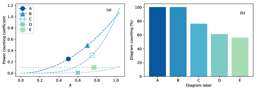
Figure 4.3: (a) The power counting coefficient as a function of the velocity gradient strength $A$, as defined from the expectation values (4.33-4.37) taken for $g=1.0$ and $\tau=0.1$. (b) Relative frequencies, within the interval $0\leq A\leq 1$, of the cases where the power counting coefficients are found to be among the first five largest ones.

It turns out that in the considered range of velocity gradient strengths, two contributions, which have exactly the same power counting coefficients, are clearly dominant over the remaining ones. These are the cumulant corrections A and B, defined in Eqs. (4.33) and (4.34). Note that the power counting coefficient for the contribution E, Eq. (4.37), is actually independent of $A$, and, therefore, plays no role at all in the evaluation of the PDFs. Diagram E is only displayed for matters of completeness, since it casually happens to be larger than many other diagrams. It is important to note that power counting is actually an effective way to identify relevant contributions, provided these are in fact dependent on the velocity gradient tensor - a fact that we check for each one of the selected diagrams.

With respect to the fluctuations, the first order contribution in the expansion around the instantons is null, $\langle\Delta S_{1}[\hat{\mathbf{A}},{\mathbf{A}}]\rangle_{0}=0$, because the instantons satisfy the Euler-Lagrange equations for the $\Delta S_{0}$ action. From this fact and Eq. (4.22), the MSRJD effective action can be written as

$$\Gamma[\hat{\mathbf{A}}^{sp},{\mathbf{A}}^{sp}]=S[\hat{\mathbf{A}}^{sp},{\mathbf{A}}^{sp}]+\sum_{n}C_{n}[\hat{\mathbf{A}}^{sp},{\mathbf{A}}^{sp}]\mbox{,}$$ (4.38)

where $n$ labels the several second order cumulant expansion terms $C_{n}[\hat{\mathbf{A}}^{sp},{\mathbf{A}}^{sp}]$, which are dominated by the contributions A and B. Their associated Feynman diagrams, represented in Fig. 4.4, are noted to renormalize the noise and propagator kernels in the effective MSRJD action (4.38).

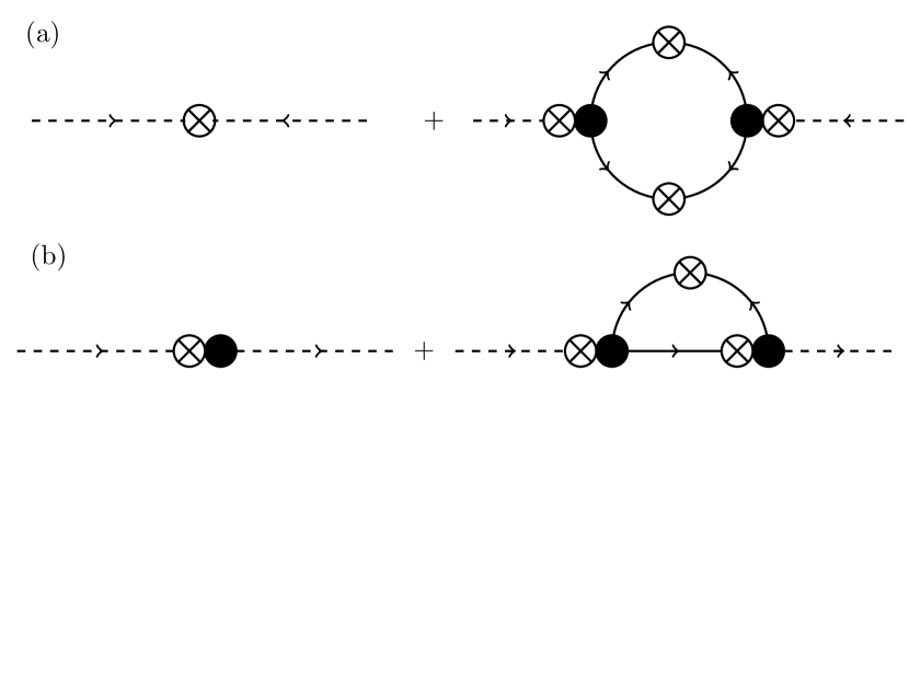
Figure 4.4: Feynman diagrams for (a) the renormalized noise and (b) the renormalized causal propagator kernels, which take into account the one-loop contributions A and B, respectively.

The contributions A and B to the effective action (4.38) can be written, more concretely, as

$$C_{\textbf{A}}[\hat{\mathbf{A}}^{sp},{\mathbf{A}}^{sp}]=\frac{1}{2}\int_{-\beta}^{0}dt\int_{-\beta}^{0}dt^{\prime}\hat{A}^{sp}_{ij}(t)\hat{A}^{sp}_{kl}(t^{\prime})C^{A}_{ijkl}(t-t^{\prime})$$ (4.39)

and

$$C_{\textbf{B}}[\hat{\mathbf{A}}^{sp},{\mathbf{A}}^{sp}]=\frac{1}{2}\int_{-\beta}^{0}dt\int_{-\beta}^{0}dt^{\prime}\hat{A}^{sp}_{ij}(t)C^{B}_{ij}({\mathbf{A}}^{sp}(t^{\prime}),t-t^{\prime})\mbox{,}$$ (4.40)

where

$$C^{A}_{ijkl}(t-t^{\prime})=\langle[V_{2}({\mathbf{A}}(t))]_{ij}[V_{2}({\mathbf{A}}(t^{\prime}))]_{kl}\rangle_{0}$$ (4.41)

and

$$C^{B}_{ij}({\mathbf{A}}^{sp}(t^{\prime}),t-t^{\prime})=\langle[V_{2}({\mathbf{A}}(t))]_{ij}\hat{A}_{kl}(t^{\prime})[\Delta V_{2}({\mathbf{A}}(t^{\prime}))]_{kl}\rangle_{0}\mbox{.}$$ (4.42)

These terms correspond to the integration over fluctuating fields.

4.3.1 Structure of the MSRJD Effective Action

The effective action (4.38) can be written, after the introduction of the contributions (4.39) and (4.40), as

$$\begin{split}\Gamma[\hat{\mathbf{A}},{\mathbf{A}}]=i\int_{-\beta}^{0}dt\int_{-\beta}^{0}dt^{\prime}\Bigg{\{}&\mathrm{Tr}\left[\hat{\mathbf{A}}^{\mathrm{T}}(t)\left(\frac{d\mathbf{A}}{dt}-V^{\mathrm{ren}}({\mathbf{A}}(t^{\prime}),t-t^{\prime})\right)\right]\\ +&\frac{g^{2}}{2}G_{ijkl}^{\mathrm{ren}}(t-t^{\prime})\hat{A}_{ij}(t)\hat{A}_{kl}(t^{\prime})\Bigg{\}}\ .\end{split}$$ (4.43)

This action has the same form as the instanton action, $S_{sp}[\hat{\mathbf{A}}^{sp},{\mathbf{A}}^{sp}]$, with two renormalized terms: the noise $G$ and the potential $V$. These renormalizations correspond to the effective role of the fluctuations to the terms in the saddle-point action. Explicitly, these contributions are

$$G_{ijkl}^{\mathrm{ren}}(t-t^{\prime})\equiv G_{ijkl}\delta(t-t^{\prime})+C^{A}_{ijkl}(t-t^{\prime})$$ (4.44)

and

$$V_{ij}^{\mathrm{ren}}({\mathbf{A}}(t^{\prime}),t-t^{\prime})\equiv V_{ij}({\mathbf{A}}(t^{\prime}))\delta(t-t^{\prime})-C^{B}_{ij}({\mathbf{A}}(t^{\prime}),t-t^{\prime})\ .\$$ (4.45)

In contrast to the original nonperturbed MSRJD action (4.23), the above renormalized form (4.43) contains kernels that depend non-trivially on a pair of time instants $t$ and $t^{\prime}$. As it is usual (sometimes in an implicit way) in renormalization group studies [3, 240, 181] , the structure of the renormalized effective action can be simplified in the case of slowly varying fields (as the instanton fields are assumed to be). This simplification is achieved through the procedure of low-frequency renormalization, which in our context consists in replacing the renormalization kernels $C^{A}_{ijkl}$ and $C^{B}_{ij}$ by singular ones, according to the prescriptions

$$C^{A}_{ijkl}(t-t^{\prime})\rightarrow\tilde{C}^{A}_{ijkl}\delta(t-t^{\prime})\ ,\$$ (4.46a)

$$C^{B}_{ij}({\mathbf{A}}(t^{\prime}),t-t^{\prime})\rightarrow\tilde{C}^{B}_{ij}({\mathbf{A}}(t^{\prime}))\delta(t-t^{\prime})\ ,\$$ (4.46b)

where

$$\tilde{C}^{A}_{ijkl}\equiv\int_{-\infty}^{\infty}dt^{\prime}C^{A}_{ijkl}(t-t^{\prime})\ ,\$$ (4.47a)

$$\tilde{C}^{B}_{ij}({\mathbf{A}}(t))\equiv\int_{-\infty}^{\infty}dt^{\prime}C^{B}_{ij}({\mathbf{A}}(t^{\prime}),t-t^{\prime})\ .\$$ (4.47b)

Substituting (4.47a) and (4.47b) in (4.44) and (4.45), the nonperturbed and the effective MSRJD actions will, then, become isomorphic to each other, provided that the tensors $G_{ijkl}$ and $V_{ij}({\mathbf{A}})$ of the nonperturbed action are mapped, respectively, to the tensors

$$\tilde{G}_{ijkl}^{\mathrm{ren}}\equiv G_{ijkl}+\tilde{C}^{A}_{ijkl}$$ (4.48)

and

$$\tilde{V}_{ij}^{\mathrm{ren}}({\mathbf{A}})\equiv V_{ij}({\mathbf{A}})-\tilde{C}^{B}_{ij}({\mathbf{A}})$$ (4.49)

that appear in the definition of the effective renormalized action.

It is important to observe, furthermore, that from the traceless property of the stochastic forcing, it follows that $\tilde{G}_{iikl}^{\mathrm{ren}}=\tilde{G}_{ijkk}^{\mathrm{ren}}=0$, and we may write, in general, that

$$\tilde{G}_{ijkl}^{\mathrm{ren}}=D_{ijkl}-\frac{1}{3}(x+y)\delta_{ij}\delta_{kl}\ ,\$$ (4.50)

where

$$D_{ijkl}=x\delta_{ik}\delta_{jl}+y\delta_{il}\delta_{jk}\ ,\$$ (4.51)

with $x$ and $y$ being two independent arbitrary parameters. The computation of the noise renormalization diagram, Fig. 4.4a, returns

$$\tilde{C}^{A}_{ijkl}=\frac{g^{4}}{8}\left(6\delta_{ik}\delta_{jl}-\frac{1}{4}\delta_{il}\delta_{jk}-\frac{23}{12}\delta_{ij}\delta_{kl}\right)\mbox{,}$$ (4.52)

and, as a consequence,

$$x=2+\frac{3}{2}g^{2}\ ,\ y=-\frac{1}{2}-\frac{1}{16}g^{2}\mbox{.}$$ (4.53)

In its turn, the renormalization of the potential produces the contribution

$$\tilde{C}^{B}_{ij}=\frac{g^{2}}{16}(4A_{ji}-A_{ij}).$$ (4.54)

The calculation of the renormalization terms in Eqs. (4.52) and (4.54) involves the manipulation of several $A_{ij}$ and $G_{ijkl}$ factors in complex tensor contractions. These tensor contractions have been performed with the computer algebra system Mathematica and they are described in Appendix A.

Recalling, now, the saddle-point to solve for $\hat{\mathbf{A}}^{sp}$ in terms of ${\mathbf{A}}^{sp}$, the MSRJD effective action can be rewritten in a more compact way, up to the same order in perturbation expansion, as a scalar functional uniquely dependent on the velocity gradient tensor field ${\mathbf{A}}$, namely,

$$\begin{split}\Gamma[{\mathbf{A}}]&=\frac{1}{2g^{2}}\int_{-\beta}^{0}dt\ \left(\frac{dA_{ij}}{dt}-\tilde{V}^{\mathrm{ren}}_{ij}({\mathbf{A}})\right)D^{-1}_{ijkl}\left(\frac{dA_{kl}}{dt}-\tilde{V}^{\mathrm{ren}}_{kl}({\mathbf{A}})\right)\\ &=\frac{a}{2g^{2}}\int_{-\beta}^{0}dt\ \left(\frac{dA_{ij}}{dt}-\tilde{V}^{\mathrm{ren}}_{ij}({\mathbf{A}})\right)\left(\frac{dA_{ij}}{dt}-\tilde{V}^{\mathrm{ren}}_{ij}({\mathbf{A}})\right)\\ &+\frac{b}{2g^{2}}\int_{-\beta}^{0}dt\ \left(\frac{dA_{ij}}{dt}-\tilde{V}^{\mathrm{ren}}_{ij}({\mathbf{A}})\right)\left(\frac{dA_{ji}}{dt}-\tilde{V}^{\mathrm{ren}}_{ji}({\mathbf{A}})\right)\ ,\end{split}$$ (4.55)

where

$$D^{-1}_{ijkl}\equiv a\delta_{ik}\delta_{jl}+b\delta_{il}\delta_{jk}\ ,\$$ (4.56)

with

$$a=-\frac{x}{y^{2}-x^{2}}\ ,\ b=\frac{y}{y^{2}-x^{2}}\ .\$$ (4.57)

In the formulation of Eq. 4.55, it is not necessary anymore to work with a coupled set of saddle-point equations. Instead, the instanton configuration is obtained from a single equation

$$\left.\frac{\delta\Gamma[{\mathbf{A}}]}{\delta A_{ij}}\right|_{{\mathbf{A}}={\mathbf{A}}^{sp}}=0\ .$$ (4.58)

The effective action of Eq. 4.55 is usually called the Onsager-Machlup action functional [172].

4.3.2 Instanton Configurations

One the working hypothesis made in [160] was the relevance of an approximate analytical instanton, instead of the exact field, solution of Eq. 4.29. In this work, the applicability of this hypothesis was verified. The approximate instantons consist in the saddle-point solutions of a quadratic truncated renormalized effective action,

$$\Gamma_{0}[{\mathbf{A}}]\equiv\frac{a}{2g^{2}}\int_{-\beta}^{0}dt\ \mathrm{Tr}\left[\dot{\mathbf{A}}^{\mathrm{T}}\dot{\mathbf{A}}+{\mathbf{A}}^{\mathrm{T}}{\mathbf{A}}\right]+\frac{b}{2g^{2}}\int_{-\beta}^{0}dt\ \mathrm{Tr}\left[\dot{\mathbf{A}}^{2}+{\mathbf{A}}^{2}\right]\ .$$ (4.59)

The corresponding approximate saddle-point equation is

$$\left.\frac{\delta\Gamma_{0}[{\mathbf{A}}]}{\delta A_{ij}}\right|_{{\mathbf{A}}={\mathbf{A}}^{sp}}=0\Rightarrow\ddot{\mathbf{A}}^{sp}-{\mathbf{A}}^{sp}=0\ ,\$$ (4.60)

subject to the periodic boundary condition (4.14). Instanton solutions of (4.60) have the form

$${\mathbf{A}}^{sp}(t)=\bar{\mathbf{A}}f(\beta,t)\mbox{,}$$ (4.61)

where the function $f(\beta,t)$, defined for $-\beta\leq t\leq 0$, is given by

$$f(\beta,t)=2\frac{\sinh(\beta/2)}{\sinh(\beta)}\cosh(t+\beta/2)\mbox{.}$$ (4.62)

Additionally, since the potential functions $V_{p}({\mathbf{A}})$ are homogeneous functions of degree $p$, their contribution conforms to

$$V({\mathbf{A}}^{sp}(t))=\sum_{p=1}^{4}V_{p}(\bar{\mathbf{A}})[f(\beta,t)]^{p}\ .$$ (4.63)

The above expression together with (4.11), (4.48) and (4.49), leads to the evaluation of the effective action (Eq. 4.55) from these following scalar contributions:

$$\begin{split}\int_{-\beta}^{0}dt\ &\left(\frac{dA_{ij}^{sp}}{dt}-V_{ij}^{\mathrm{ren}}(\mathbf{A}^{sp})\right)\left(\frac{dA_{ij}^{sp}}{dt}-V_{ij}^{\mathrm{ren}}(\mathbf{A}^{sp})\right)=\\ &I_{1}(\beta)\mathrm{Tr}[\bar{\mathbf{A}}^{\mathrm{T}}\bar{\mathbf{A}}]+\sum_{p=1}^{4}\sum_{q=1}^{4}I_{p+q}(\beta)H_{p,q}(\bar{\mathbf{A}}^{\mathrm{T}},\bar{\mathbf{A}})\end{split}$$ (4.64)

and

$$\begin{split}\int_{-\beta}^{0}dt\ &\left(\frac{dA_{ij}^{sp}}{dt}-V_{ij}^{\mathrm{ren}}(\mathbf{A}^{sp})\right)\left(\frac{dA_{ji}^{sp}}{dt}-V_{ji}^{\mathrm{ren}}(\mathbf{A}^{sp})\right)=\\ &I_{1}(\beta)\mathrm{Tr}[\bar{\mathbf{A}}^{2}]+\sum_{p=1}^{4}\sum_{q=1}^{4}I_{p+q}(\beta)H_{p,q}(\bar{\mathbf{A}},\bar{\mathbf{A}})\ ,\ \end{split}$$ (4.65)

where $H_{p,q}(X,Y)$ is an homogeneous scalar function of degrees $p$ and $q$, related, respectively, to the matrix variables $X$ and $Y$, and

$$I_{1}(\beta)\equiv\int_{-\beta}^{0}dt[\dot{f}(\beta,t)]^{2}\mbox{,}\ I_{p+q}(\beta)\equiv\int_{-\beta}^{0}dt[f(\beta,t)]^{p+q}\mbox{.}$$ (4.66)

At asymptotic times, $\beta\rightarrow\infty$, the constants $I_{p}$ are defined as $I_{p}=\lim_{\beta\rightarrow\infty}I_{p}(\beta)$ and their exact values are:

$$\begin{split}&I_{1}=I_{2}=1\mbox{,}\ I_{3}=2/3\mbox{,}\ I_{4}=1/2\mbox{,}\\ &I_{5}=2/5\mbox{,}\ I_{6}=1/3\mbox{,}\ I_{7}=2/7\mbox{,}\ I_{8}=1/4\mbox{.}\end{split}$$

Assembling all the above pieces together, the effective action is

$$\begin{split}\Gamma[{\mathbf{A}}^{sp}]\equiv\Gamma(\bar{\mathbf{A}})&=\frac{aI_{1}}{2g^{2}}\mathrm{Tr}[\bar{\mathbf{A}}^{\mathrm{T}}\bar{\mathbf{A}}]+\frac{bI_{1}}{2g^{2}}\mathrm{Tr}[\bar{\mathbf{A}}^{2}]\\ &+\sum_{p=1}^{4}\sum_{q=1}^{4}\frac{I_{p+q}}{2g^{2}}[aH_{p,q}(\bar{\mathbf{A}}^{\mathrm{T}},\bar{\mathbf{A}})+bH_{p,q}(\bar{\mathbf{A}},\bar{\mathbf{A}})]\ .\ \end{split}$$ (4.67)

The normalized vgPDF can now be readily derived from (4.21) and (4.67), therefore, as

$$\rho(\bar{\mathbf{A}})={\cal{N}}\exp[-\Gamma(\bar{\mathbf{A}})]\ .\$$ (4.68)

It is relevant to compare the approximate instanton solutions (Eq. 4.61) with accurate numerical solutions in specific cases. As discussed in [96], diagonal velocity gradient instantons can be obtained from the application of the Chernykh-Stepanov method [36] for the particular boundary conditions,

$$\begin{split}&\bar{A}_{11}=-2\bar{A}_{22}=-2\bar{A}_{33}\equiv c\ ,\ \\ &\bar{A}_{ij}=0{\hbox{ for $i\neq j$}}\ ,\ \end{split}$$ (4.69)

where $c$ is an arbitrary constant. The approximate and the numerical instantons for $c=1$, $\tau=0.1$, and $g=0.8$ are both plotted in Fig. 4.5, for three different values of the $\beta$ parameter. This figure reveals that the approximate instantons are uniformly close to the exact ones, justifying the use of quadratic instantons in the analytical approach. It is also worth pointing out that the regime in question is that of moderate Reynolds numbers and fluctuations only a few standard deviations from the mean, which does not guarantee the same uniform agreement for high Reynolds numbers. The use of approximate instantons also implies, in an exact formulation, that the first order contribution $\langle\Delta S_{1}\rangle_{0}$ is not zero, but these contributions can be safely discarded due to their low relevance in the power counting scheme, and by the small difference between the exact and numerical instantons.

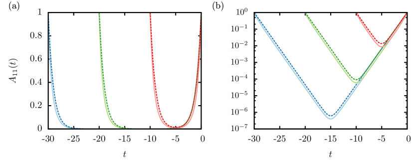
Figure 4.5: Comparison between approximate (dashed lines) and numerical instantons (solid lines), obtained, respectively from Eq. (4.61) and from the application of the Chernykh-Stepanov method as discussed in [96], for $c=1$ [that is $\bar{A}_{11}=1$, see Eq. (4.69)], $\tau=0.1$, and $g=0.8$ in (a) linear and (b) monolog scales. Notice that the approximate and the numerical instantons both refer to the RFD model. Blue, green and red curves (left to right) correspond to $\beta=30$, $20$ and $10$.

4.4 Numerical Results

This section discusses the analytical predictions obtained from the renormalized effective action in comparison to the numerical results obtained directly from the RFD model. The observables considered have been previously studied in the context of Lagrangian velocity gradients and reveal many of the non-trivial features of their dynamics.

The PDF in Eq. 4.68 is multivariate, it is defined on the domain of nine velocity gradient components. But symmetries between the components yield redundant the individual analysis of all of them. The high-dimensionality of the problem also makes it impractical to consider the whole distribution. For this reason, marginal PDFs have been produced from statistical ensembles of velocity gradients generated with a Monte Carlo procedure. The detailed procedure to sample configurations from the effective action $\Gamma[\hat{\mathbf{A}}^{sp},{\mathbf{A}}^{sp}]$ is described in [160].

The Monte Carlo samples consisted of sets of $8\times 10^{6}$ velocity gradient tensors, from which were extracted ensembles of $24\times 10^{6}$ and $48\times 10^{6}$ diagonal and off-diagonal velocity gradient components, respectively. An illustrative case for the marginal PDFs of the diagonal and off-diagonal components of the velocity gradient tensor is given in Fig. 4.6, for controlling parameters $\tau=0.1$ and $g=0.8$. For this value of $\tau$, the RFD model leads to statistical results similar to the ones observed in realistic turbulent flows [39].

The PDFs of velocity gradients are compared in four different situations:

1. the straightforward numerical simulations of the RFD model, Eq. (4.5) with the potential from Eq. (4.8). This statistical ensemble contains $10^{9}$ velocity gradient tensors, covering $2\times 10^{5}$ integral times scales,

2. the saddle-point MSRJD action with no renormalization contributions, $S_{sp}[\hat{\mathbf{A}}^{sp},{\mathbf{A}}^{sp}]$.

3. the partial renormalization of the effective MSRJD action, which is renormalized only by the noise contribution, as given by Eqs. (4.43) and (4.44), with $\tilde{C}^{B}_{ij}=0$ prescribed in (4.45), and

4. the full renormalization of the effective action, which is renormalized by both the noise and the propagator contributions, as given by Eqs. (4.43), (4.44), and (4.45).

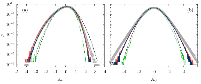
Figure 4.6: PDFs for the (a) diagonal and (b) off-diagonal velocity gradient components, computed for $\tau=0.1$ and $g=0.8$. Open squares refer to the empirical PDFs derived from the numerical solutions of the RFD model, while all the other PDFs follow from analytical expressions obtained at different improvement levels. Green dashed lines correspond to no effective action renormalization, red (light gray) lines to partial renormalization and blue (dark gray) lines to full renormalization. The dotted-dashed gray lines correspond to Gaussian fits of the numerical (RFD) data around the PDFs peaks, which clearly show deviations from quadratic behavior both in the partial and full renormalization schemes. The diagonal and off-diagonal empirical PDFs have standard deviations and kurtosis given by $\sigma=0.66$ and $\kappa=3.3$ and $\sigma=0.89$ and $\kappa=3.7$, respectively.

In Fig. 4.6, it can be seen that great improvement is obtained with the use of renormalized actions. Noise renormalization is found to be the leading contribution, and for this reason we may refer to the propagator renormalization contribution as the subleading one. The results from partial and full renormalization, though, seem essentially equivalent, with small differences observed mainly for the PDF tails of diagonal velocity gradient components. In closer inspection, though, it is found that the core regions of the numerical distribution is more accurately described by the PDF from the complete renormalization procedure.

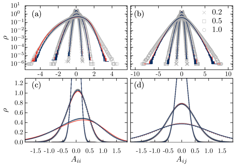
Figure 4.7: PDFs for the diagonal components of the velocity gradient tensor at (a) and (c), and its off-diagonal components, at (b) and (d). Figures (a) and (b) are in monolog scale, while figures (c) and (d) are in linear scale, and they represent the same sets of data. Symbols refer to the empirical PDFs derived from the numerical solutions of Eq. (4.5), for different values of the random force strength $g$, as indicated in the plots; red (light gray) and blue (dark gray) lines refer, respectively, to PDFs obtained from partial and fully renormalized effective actions. With better visualization in mind, the non-renormalized PDFs have not been plotted.

A more extensive comparison between PDFs is provided in Fig. 4.7, where the cores of these distributions are examined with more care. In this figure, three values of $g$ are chosen, up to $g=1.0$, which is close to the limit of validity of perturbation theory. This upper limit can be estimated from the perturbative corrections (4.53) and appreciated from the results of simulations: above $g=1.0$ the renormalized PDFs are noted to deviate in a more expressive way from the numerical ones. It is to be remarked here that the definition of an upper bound for the coupling constant $g$ is by no means a sufficient condition for the validity of the perturbative expansion, since it is important that both $g$ and $A$ are not too large for the consistency of the cumulant expansion approach. There is a clear interplay between these quantities, since the variance of $A$ scales as $g^{2}$ for small values of $g$, though this yields interesting information only around the PDF peaks.

Standard Deviations
g	0.2		0.5		1.0
Statistical Ensembles	D	OD	D	OD	D	OD
Numerical RFD	0.14	0.20	0.39	0.52	0.86	1.15
No Renormalization	0.14	0.20	0.35	0.48	0.68	0.88
Partial Renormalization	0.14	0.20	0.39	0.52	0.90	1.13
Full Renormalization	0.14	0.20	0.39	0.52	0.84	1.13

Kurtoses
g	0.2		0.5		1.0
Statistical Ensembles	D	OD	D	OD	D	OD
Numerical RFD	3.05	3.03	3.25	3.23	3.23	3.87
No Renormalization	3.03	3.01	3.12	3.09	3.19	3.33
Partial Renormalization	3.03	3.01	3.14	3.12	3.14	3.51
Full Renormalization	3.03	3.01	3.14	3.10	3.14	3.39

Table 4.1: Standard deviations and kurtoses associated to the vgPDFs shown in Fig. 4.7. The labels D and OD stand for statistical ensembles of diagonal and off-diagonal velocity gradient components, respectively. These ensembles are characterized, besides the D/OD classification, from specifying how their associated PDFs are obtained, according to four alternative schemes, described as the items (i) to (iv) in Sec. 4.4: numerical simulations of the RFD model, non-renormalized saddle-point MSRJD actions, partially renormalized effective actions, and fully renormalized effective actions.

The standard deviations and kurtoses of these PDFs are reported in Table 4.1. It is verified that the standard deviations agree remarkably well with those evaluated directly from the RFD model. The comparison between kurtoses, on the other hand, has some discrepancies, mainly due to the slow decay of the far tails of the PDFs, which are out of the reach of the present approach.

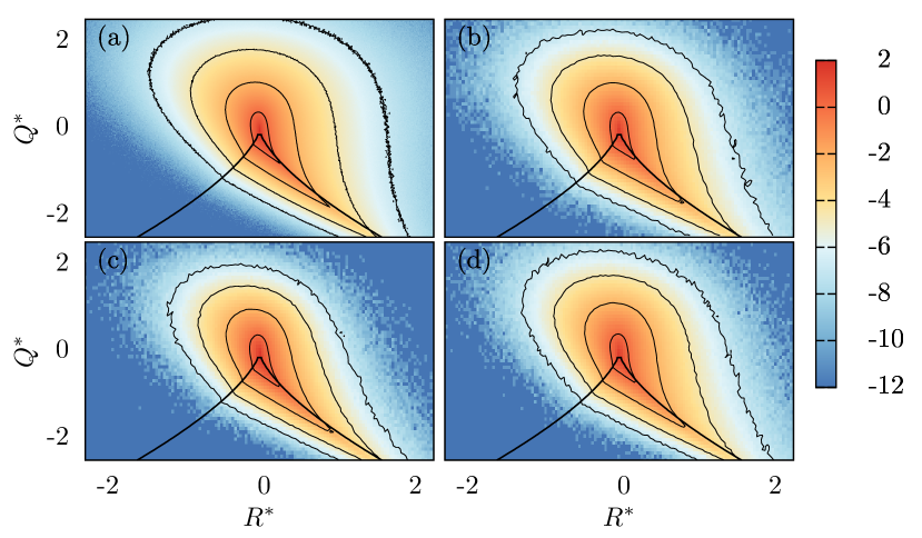
Figure 4.8: Joint PDFs (and their level curves) of the velocity gradient invariants $Q^{*}$ and $R^{*}$, as obtained from (a) numerical simulations of the RFD model, (b) the analytical approach based on the non-renormalized effective MSRJD action, (c) the noise renormalized effective action and (d) the fully renormalized effective action. Solid lines represent the “Vieillefosse line”, defined by $(27/4)R^{2}+Q^{3}=0$ (a constraint which holds for the inviscid evolution of the velocity gradient tensor). The data correspond to the RFD parameters $\tau=0.1$ and $g=0.8$, and the color bar scale corresponds to powers of 10 in the visualization of the joint probability distribution functions.

The pair of velocity gradient invariants $Q\equiv-\mathrm{Tr}({\mathbf{A}}^{2})/2$ and $R\equiv-\mathrm{Tr}({\mathbf{A}}^{3})/3$ have been extensively used in the literature as important observables for the investigation of structural aspects of turbulence [221]. Turbulent flow regions can be dominated by enstrophy ($Q>0$) or strain ($Q<0$) and, independently, by compression ($R>0$) or stretching ($R<0$) dynamics. It is interesting to work with a dimensionless version of these invariants,

$$Q^{*}=-\frac{\mathrm{Tr}({\mathbf{A}}^{2})}{2\langle\mathrm{Tr}(\mathbf{S}^{2})\rangle}\ \ \mbox{and}\ \ R^{*}=-\frac{\mathrm{Tr}({\mathbf{A}}^{3})}{3\langle\mathrm{Tr}(\mathbf{S}^{2})\rangle^{3/2}}\mbox{,}$$ (4.70)

where $\mathbf{S}=({\mathbf{A}}+{\mathbf{A}}^{\mathrm{T}})/2$ is the strain rate tensor, the symmetric part of the velocity-gradient tensor. The joint PDF of $Q^{*}$ and $R^{*}$ shows a characteristic teardrop shape, which was first observed in direct numerical simulations of turbulence [137, 227, 228]. This teardrop shape is qualitatively well reproduced by the RFD model [39].

With the same Monte Carlo ensembles used to produce the marginal PDFs, the joint PDF of $Q^{*}$ and $R^{*}$ was produced in the same four regimes, and the relevance of renormalization can be observed for this observable too, as can be seen in Fig. 4.8. In particular, the difference between the leading order (Fig. 4.8c) and complete renormalization (Fig. 4.8d) is noticeable, since the latter is much closer to the numerical results (Fig. 4.8a) than the former.

4.5 Discussion

The results of [160] motivated this deeper analysis of the field theoretical approach to the RFD approach, a model of Lagrangian intermittency [39]. The work described in this chapter, [6], pursued a detailed verification of approximation hypotheses which were made in this previous work.

Notably, two main results stand out: The accuracy of the quadratic instanton, which is used as a proxy for the exact instanton, was verified. And the ranking of the relevance of each diagram was established, advocating for the relevance of the noise renormalization which was empirically observed in [160].

The cumulant expansion yields accurate results for the core of PDFs at the onset of turbulence, as observed. That is, in regimes of moderate Reynolds numbers, where fat tails start to stand out. In this situation, the expansion is a reliable perturbation technique. At the far PDF tails, on the other hand, the perturbative expansion breaks down, and asymptotically large fluctuations are instead well described purely by the instantons, thus requiring an exact treatment of the saddle-point solutions.

Chapter 5 The Onset of Intermittency in Stochastic Burgers Hydrodynamics

The Burgers model was introduced in [30] as a one-dimensional prototype for Navier-Stokes hydrodynamics. It displays nonlinearities which are similar to those of Navier-Stokes, and became a valuable testing ground for the development of new theoretical and computational approaches in turbulence and hydrodynamics, as foreseen in [165]. Furthermore, the Burgers equation has been applied to realistic problems in a variety of fields: nonlinear acoustics [98], cosmology [238, 99], critical interface growth [117], traffic flow dynamics [161, 40], and biological invasion [182].

The stochastic Burgers model determines the evolution of the velocity field $u(x,t)$ which is forced by a random external force $\phi(x,t)$:

$$u_{t}+uu_{x}=\nu u_{xx}+\phi\ ,\$$ (5.1)

As usual, $\nu$ is the kinematic viscosity. And similarly to Navier-Stokes, observables such as velocity gradients, $\xi=\partial_{x}u$, and velocity differences, $\delta u_{\ell}(x)=u(x+\ell)-u(x)$, display intermittent fluctuations in turbulent steady state solutions.

Starting from a smooth initial condition, this model leads to the formation of smooth ramps and sudden negative shocks, which can be seen in Fig. 5.1a. The probability distribution of the velocity gradient, seen in Fig. 5.1b, can also be understood from the picture of ramps and shocks: Positive velocity gradients are small and with little fluctuations, while negative gradients are extremely intermittent, with the largest negative fluctuations forming visible shocks.

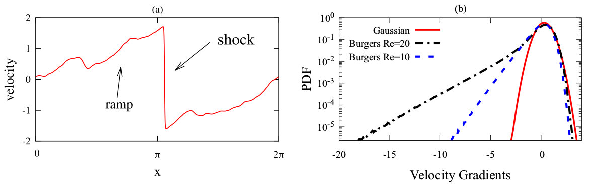
Figure 5.1: Burgers hydrodynamics is marked by the formation of sudden negative shocks interleaved by smooth positive ramps. A ramp and a shock are identified in (a). This dynamics leads to the PDF observed in (b), where positive gradients decay fast, while negative gradients display intense fluctuations, which grow with higher Reynolds numbers. A comparison between these PDFs and a Gaussian distribution is also shown. This figure was extracted from [145].

The instanton approach was applied to the Burgers model in [97], where it was shown that the velocity difference PDFs followed

$$\rho_{g}(\delta u)=\exp[-S(\delta u)]\ ,$$ (5.2)

and that the asymptotic form of the action $S(\xi)$ was

$$S(\delta u)\sim|\delta u|^{3}\ .$$ (5.3)

This result confirms that fluctuations in the positive tails are effectively irrelevant, since their distribution is sub-Gaussian. As a consequence, the instanton PDF is essentially exact. The same result had been obtained before by different methods in [184]. Furthermore, the exponent $3$ is equally observed for positive velocity gradients, a result demonstrated in [91].

Negative fluctuations, though, due to their intermittent fluctuations, are still subject of research in this field. The first result on negative gradients with the instanton method was obtained in [13], where it was demonstrated that the left tail of the velocity gradient probability distribution could be written as Eq. (5.2), but instead depending on $\xi$. The asymptotic behavior of the PDF tails is given by

$$S(\xi)\sim|\xi|^{\frac{3}{2}}\ ,$$ (5.4)

which corresponds to a fat tailed distribution. The hypotheses made in these calculations and the general result were verified in [36], although, as [93] point out, the asymptotic form of $S(\xi)$ is still beyond the reach of direct numerical simulations. Still, the authors observe an agreement between the velocity gradient PDF tails and those provided by the instanton configurations. This agreement, however, relies on an arbitrary multiplication of the random force strength parameter by a Reynolds number dependent adjustment factor. A detailed analytical investigation on why such an empirical “noise renormalization procedure” works is the central aim of the work developed in [7], work on which this chapter is based.

5.1 Field Theoretical Setup

A dimensionless version of Burgers equation is obtained by equivalent methods to those of Section 2.2, by measuring length in units of $L$, the forcing scale, time in units of $L^{2}/\nu$ and velocity in units of $\nu/L$. As a result:

$$u_{t}+uu_{x}-u_{xx}=g\phi\ ,\$$ (5.5)

where $\phi=\phi(x,t)$ is a zero-mean Gaussian random field used to model large-scale forcing, with correlator

$$\langle\phi(x,t)\phi(x^{\prime},t^{\prime})\rangle=\chi(x-x^{\prime})\delta(t-t^{\prime})\ .\$$ (5.6)

The correlation function $\chi$ is peaked at wavenumber $k=0$ and broadened in Fourier space within a region of size $\Delta k\sim 1$. In other words, $L\equiv 1$ ($\sim\Delta k^{-1}$) is taken to be the random force correlation length, defined as the largest relevant length scale in the flow. While most of the considerations in this section are general, a specific form of the correlation function is adopted, as it has been addressed in former works [13, 91, 93],

$$\chi(x)=(1-x^{2})\exp\left(-\frac{x^{2}}{2}\right)=-\partial_{x}^{2}\exp\left(-\frac{x^{2}}{2}\right)\ .\$$ (5.7)

This is a case study of particular interest, due to its simple formulation and good analytical properties.

Note that the intensity of forcing is given by the noise strength parameter $g$. This is the only dimensionless parameter in the problem, and can be connected to the Reynolds number through the phenomenology of Section 2.5. The amplitude $\chi_{0}=\chi(0)$ of the external force correlation function is in direct correspondence with the kinetic energy dissipation rate, $\varepsilon$. Furthermore from the K41 theory, $\varepsilon\propto U^{3}/L$, where $U$ is a typical velocity. From these relations, the following dimensionally correct relation is obtained:

$$U=(\chi_{0}L)^{1/3}\ .$$ (5.8)

This equation is used to write the Reynolds number, $\mathrm{Re}=UL/\nu$ in terms of the dimensional parameters of the problem. Finally, the force strength can also be written in terms of the same parameters, as $g=\chi_{0}^{1/2}L^{2}\nu^{-3/2}$, from which it is obtained that

$$g=\mathrm{Re}^{3/2}\ .$$ (5.9)

With the Burgers model in mind, velocity gradients are going to be computed in the MSRJD formalism as path-integrations over the velocity field $u(x,t)$ and its conjugate auxiliary field $p(x,t)$, combined with an ordinary integration over a Lagrange multiplier variable $\lambda$ as

$$\rho_{g}(\xi)=\langle\delta(u_{x}|_{0}-\xi)\rangle={\cal{N}}^{-1}\int DpDu\int_{-\infty}^{\infty}d\lambda\exp\{-S[u,p,\lambda;g]\}\ ,\$$ (5.10)

where $\cal{N}$ is an unimportant normalization constant (to be suppressed from now on, in order to simplify notation), $u_{x}|_{0}$ is the velocity gradient taken at $(x,t)=(0,0)$, and $S[u,p,\lambda;g]$ is the MSRJD action:

$$\begin{split}&S[u,p,\lambda;g]=\frac{g^{2}}{2}\int dtdx~{}p(\chi*p)+\\ &+i\int dtdx~{}p(u_{t}+uu_{x}-u_{xx})-i\lambda(u_{x}|_{0}-\xi)\ ,\ \end{split}$$ (5.11)

with $\chi*p\equiv\int dx^{\prime}\chi(x-x^{\prime})p(x^{\prime},t)$, which is a convolution in space, equivalent to the one defined in Sec. 3.

The saddle-point method is adopted to find the asymptotic form of velocity gradient PDF tails. The method provides meaningful answer in cases where the PDF tails decay faster than a simple exponential, $\exp(-c|\xi|)$ for any arbitrary $c>0$, as observed in numerical studies of Burgers turbulence [91]. The saddle-point configurations $u^{c}$, $p^{c}$, and $\lambda^{c}$ that extremize the MSRJD action are named instantons and they were first obtained for the Burgers mode in [97, 68]. As pointed out in the previous chapters, they are the solutions of the Euler-Lagrange equations, which in the present case are:

$$\left.\frac{\delta S}{\delta u}\right|_{u^{c},p^{c},\lambda^{c}}\!\!\!\!\!\!\!=0\ \ \ ,\ \ \ \left.\frac{\delta S}{\delta p}\right|_{u^{c},p^{c},\lambda^{c}}\!\!\!\!\!\!\!=0\ \ \mbox{and}\ \ \left.\frac{\partial S}{\partial\lambda}\right|_{u^{c},p^{c},\lambda^{c}}\!\!\!\!\!\!\!=0\ .\$$ (5.12)

It is convenient to rescale $p(x,t)$ and $\lambda$ as

$$p\rightarrow\frac{p}{g^{2}}\ \ \mbox{and}\ \ \lambda\rightarrow\frac{\lambda}{g^{2}}\mbox{,}$$ (5.13)

so that the MSRJD action in (5.10) is rescaled as

$$S[u,p,\lambda;g]\rightarrow\frac{1}{g^{2}}S[u,p,\lambda;1]$$ (5.14)

and the Euler-Lagrange equations stated in (5.12) become

$$u_{t}^{c}+u^{c}u_{x}^{c}-u^{c}_{xx}=i\chi*p^{c}\ ,\$$ (5.15a)

$$p^{c}_{t}+u^{c}p^{c}_{x}+p^{c}_{xx}=\lambda^{c}\delta(t)\delta^{\prime}(x)\ ,\$$ (5.15b)

$$\xi=u^{c}_{x}|_{0}\ .\$$ (5.15c)

It is relevant to notice that the noise strength $g$ has been factored out of the action in Eq. (5.14). Furthermore, the saddle-point solutions $p^{c}(x,t)$ and $\lambda^{c}$ are purely imaginary, since it is natural to expect purely real velocity instantons $u^{c}(x,t)$.

When dealing with instantons, one needs, in general, to worry about the existence of degenerate families of saddle-point solutions, associated with symmetries of the action, like translation or gauge invariance. The Fadeev-Popov method is the usual procedure to eliminate such redundant solutions [41, 159]. However, in the formalism addressed here, the degeneracy issue is bypassed through the explicit assignment of the spacetime point $(x,t)=(0,0)$ as the symmetry center around which the instantons evolve, making Eqs. (5.15a) and (5.15b) not translationally invariant.

The sign of the dissipation term in Eqs. (5.15a) and (5.15b) works as an effective time-reversal: The equation for $u^{c}$ has to be solved forward in time, since it has the same sign as the standard Burgers equation, but the equation for $p^{c}$ has a reversed sign in the dissipation term, making it similar to a backward in time Burgers equation. The time domain of these solutions is $-\infty<t\leq 0$, with $u^{c}(x,-\infty)=p^{c}(x,-\infty)=0$, and the additional boundary conditions given by Eq. (5.15c) and $p^{c}(x,0^{+})=0$. The last of these is equivalent to $p^{c}(x,0^{-})=-\lambda\delta^{\prime}(x)$, or, in Fourier space, to $\tilde{p}^{c}(k,0^{-})=-i\lambda k$ [97].

Making use of this time reversal analogy, a fruitful self-consistent numerical strategy for the above saddle-point equations was proposed in [36]. This is now usually called the Chernykh-Stepanov method. One first neglects the boundary condition (5.15c), and trades it for an arbitrary fixed value of $\lambda$. The equations, then, are solved through an iterative method which, if convergent, leads to arbitrarily precise solutions.

Beginning with $u_{1}(x,t)\equiv 0$, Eq. (5.15b) is solved backwards in time for $p_{1}(x,t)$. This field, $p_{1}(x,t)$, is then used in Eq. (5.15a) to obtain $u_{2}(x,t)$. This procedure can be carried on indefinitely, and the solutions $u^{c}(x,t)$ and $p^{c}(x,t)$ can be found within a previously defined precision metric. The velocity gradient $\xi$ is defined, a posteriori, from Eq. (5.15c), as a derivative of the last iterated velocity field. It has been observed numerically that $\xi$ is a monotonically increasing function of $\lambda$, hence Eq. (5.15c) has a unique solution in this situation. It is imperative to note, though, that the Chernykh-Stepanov method may require further numerical devices to attain convergence for $|\lambda|$ large enough.

Once $u^{c}(x,t)$, $p^{c}(x,t)$ and $\lambda^{c}$ are available, an expansion around the instantons is performed, introducing the fluctuations $u(x,t)$, $p(x,t)$ and $\lambda$, along the lines of Eq. (3.36):

$$u(x,t)\rightarrow u^{c}(x,t)+u(x,t)\ ,\$$ (5.16a)

$$p(x,t)\rightarrow p^{c}(x,t)+p(x,t)\ ,\$$ (5.16b)

$$\lambda\rightarrow\lambda^{c}+\lambda\ .\$$ (5.16c)

This substitution rewrites the MSRJD action, accordingly, as

$$\begin{split}&S[u,p,\lambda;1]\rightarrow S[u^{c}+u,p^{c}+p,\lambda^{c}+\lambda;1]\\ &\equiv S_{c}[u^{c},p^{c}]+S_{0}[u,p]+S_{1}[u^{c},u,p^{c},\lambda]\ ,\ \end{split}$$ (5.17)

where $S_{c}$, $S_{0}$, and $S_{1}$ are, respectively: the saddle-point action; the sum of all quadratic forms in the $u$ and $p$ fields that do not depend on $p^{c}$ and $u^{c}$; and finally, $S_{1}$ is the contribution that collects all terms that have not been included in $S_{c}$ or $S_{0}$. Explicitly, these terms are

$$\begin{split}S_{c}&\equiv\frac{1}{2}\int dtdx~{}p^{c}(\chi*p^{c})+i\int dtdx~{}p^{c}(u^{c}_{t}+u^{c}u^{c}_{x}-u^{c}_{xx})\\ &=({\hbox{using Eq. (\ref{sp1})}})=-\frac{1}{2}\int dtdx\ p^{c}(\chi*p^{c})\ ;\\ S_{0}&=\int dtdx\left\{\frac{1}{2}\ p(\chi*p)+i\ p(u_{t}-u_{xx})\right\}\ ;\\ \end{split}$$ (5.18)

and, up to second order in the fluctuating fields:

$$S_{1}=i\int dtdx\left\{p^{c}uu_{x}-p_{x}u^{c}u\right\}-i\lambda u_{x}|_{0}\ .\$$ (5.19)

It is clear that $S_{c}$ is a functional of the instanton fields, which on their turn depend on the velocity gradient $\xi\equiv u^{c}_{x}|_{0}$. Hence we can write, more synthetically, that $S_{c}=S_{c}(\xi)$.

Now, taking into account the instanton solutions, we can reformulate the velocity gradient PDF, Eq. (5.10), as

$$\begin{split}\rho_{g}(\xi)&=\exp\left(-\frac{1}{g^{2}}S_{c}(\xi)\right)\int DpDu\int_{-\infty}^{\infty}d\lambda\exp\left[-\frac{1}{g^{2}}(S_{0}+S_{1})\right]\\ &\propto\exp\left(-\frac{1}{g^{2}}S_{c}(\xi)\right)\int_{-\infty}^{\infty}d\lambda\left\langle\exp\left(-\frac{1}{g^{2}}S_{1}\right)\right\rangle_{0}\ ,\ \end{split}$$ (5.20)

where $\langle\ \bm{\cdot}\ \rangle_{0}$ stands for an expectation value computed in the linear stochastic model defined by the MSRJD action $S_{0}$.

A perturbative development of the above expression is possible in cases where the fluctuation-dependent contributions are small relative to the leading saddle-point results, that is,

$$S_{c}(\xi)\gg g^{2}\left|\ln\left[\int_{-\infty}^{\infty}d\lambda\left\langle\exp\left(-\frac{1}{g^{2}}S_{1}\right)\right\rangle_{0}\right]\right|\ .$$ (5.21)

Therefore, the cumulant expansion is a natural method for evaluating Eq. (5.20) in a perturbative manner. Considering contributions up to second order in the instanton fields and $\lambda$, we obtain

$$\left\langle\exp\left(-\frac{1}{g^{2}}S_{1}\right)\right\rangle_{0}=\exp\left\{-\frac{1}{g^{2}}\langle S_{1}\rangle_{0}+\frac{1}{2g^{4}}\left[\langle(S_{1})^{2}\rangle_{0}-\langle S_{1}\rangle_{0}^{2}\right]\right\}\ ,$$ (5.22)

which is used to establish the effective MSRJD action,

$$\Gamma\equiv S_{c}+\langle S_{1}\rangle_{0}-\frac{1}{2g^{2}}\left[\langle(S_{1})^{2}\rangle_{0}-\langle S_{1}\rangle_{0}^{2}\right]\ .\$$ (5.23)

The basic building blocks needed to evaluate (5.22) are the correlation functions

$$\begin{split}G_{pu}(x,x^{\prime},t,t^{\prime})&\equiv\langle p(x,t)u(x^{\prime},t^{\prime})\rangle_{0}\\ &=-\frac{ig^{2}}{2\sqrt{\pi(t^{\prime}-t)}}\exp\left[-\frac{(x-x^{\prime})^{2}}{4(t^{\prime}-t)}\right]\Theta(t^{\prime}-t)\end{split}$$ (5.24)

and

$$\begin{split}G_{uu}(x,x^{\prime},t,t^{\prime})&\equiv\langle u(x,t)u(x^{\prime},t^{\prime})\rangle_{0}\\ &=\frac{g^{2}}{2\sqrt{1+2|t-t^{\prime}|}}\exp\left[-\frac{(x-x^{\prime})^{2}}{2(1+2|t-t^{\prime}|)}\right]\ .\ \end{split}$$ (5.25)

The first propagator connects the velocity field and the auxiliary field, while the second connects two velocity fields at different positions and instants. Thus, these propagators are equivalent to those described for the RFD model, and illustrated in Fig. 4.1.

From Eqs. (5.24) and (5.25), it can be shown that $\langle S_{1}\rangle_{0}=0$ and

$$\langle(S_{1})^{2}\rangle_{0}=I_{1}[p^{c},u^{c}]+I_{2}[p^{c}]-\lambda^{2}\langle(u_{x}|_{0})^{2}\rangle_{0}\ ,\$$ (5.26)

with

$$I_{1}[p^{c},u^{c}] \equiv\int_{t,t^{\prime}<0}dtdt^{\prime}dxdx^{\prime}~{}p^{c}(x,t)u^{c}(x^{\prime},t^{\prime})H_{1}(x,x^{\prime},t,t^{\prime})\ ,$$ (5.27a)

$$I_{2}[p^{c}] \equiv\int_{t,t^{\prime}<0}dtdt^{\prime}dxdx^{\prime}~{}p^{c}(x,t)p^{c}(x^{\prime},t^{\prime})H_{2}(x,x^{\prime},t,t^{\prime})\ ,$$ (5.27b)

where

$$\begin{split}&H_{1}(x,x^{\prime},t,t^{\prime})=-2\partial_{x}[G_{uu}(x,x^{\prime},t,t^{\prime})\partial_{x}G_{pu}(x^{\prime},x,t^{\prime},t)]\ ,\ \\ &H_{2}(x,x^{\prime},t,t^{\prime})=\frac{1}{2}\partial_{x}^{2}[G_{uu}(x,x^{\prime},t,t^{\prime})]^{2}\ .\ \end{split}$$ (5.28)

Note that $I_{1}[p^{c},u^{c}]$ and $I_{2}[p^{c}]$, both of $O(g^{4})$, are the one-loop contributions which renormalize, respectively, the heat and noise kernels of the original stochastic Burgers equation, Eq. (5.5). These corrections are also equivalent to those for the RFD model, represented in Fig. 4.4, in the previous chapter.

The overall effect of perturbative contributions can always be conventionally accounted by a redefinition of the noise strength parameter $g$ in the expression for the velocity gradient PDF, $\rho_{g}(\xi)\propto\exp(-S_{c}(\xi)/g^{2})$. In the present context, the $g$-independent coefficient

$$c(\xi)\equiv-\frac{I_{1}[p^{c},u^{c}]+I_{2}[p^{c}]}{2g^{4}S_{c}}\$$ (5.29)

is enough. Using (5.20), (5.22), and integrating over $\lambda$ in the Gaussian approximation given by (5.26), a renormalized expression for the velocity gradient PDF is obtained,

$$\rho_{g}(\xi)\propto\exp\left(-\frac{S_{c}(\xi)}{g_{R}^{2}}\right)\ ,\$$ (5.30)

in which

$$g_{R}\equiv\frac{g}{\sqrt{1+c(\xi)g^{2}}}$$ (5.31)

defines an effective noise strength parameter, which is, in principle, a velocity-gradient dependent quantity that encodes the effects of fluctuations around the instantons, up to the lowest non-trivial order in the cumulant perturbative expansion.

5.2 The Onset of Intermittency

Eq. (5.31) suggests, in fact, a simple criterion for the consistency of the perturbative analysis. The cumulant expansion is meaningful, up to second order, if $|c(\xi)|g^{2}$ is reasonably smaller than unity. It follows, immediately, that for any fixed velocity gradient $\xi$, the cumulant expansion will break down for $g$ large enough. Similarly, since (as will be seen) $c(\xi)$ is a positive monotonically increasing function of $|\xi|$, the cumulant expansion framework becomes inadequate for large enough $|\xi|$ at any fixed $g$.

Consequently, the consideration of strong coupling regimes ($g\gg 1$, equivalent to high Reynolds numbers) and/or asymptotically large velocity gradient fluctuations is precluded from the cumulant expansion approach. The perturbative analysis, nevertheless, is actually useful to model the shape of velocity gradient PDF left tails in the non-Gaussian region, where $|\xi|>g$, for not very large $g$. It is expected that, as the noise strength grows and incipient turbulent fluctuations associated to flow instabilities come into play, the onset of non-Gaussian behavior is captured by dominant instanton contributions “dressed” by cumulant corrections.

It is important, before proceeding, to comment on the challenging technical difficulties associated to the evaluations of $S_{c}(\xi)$, $I_{1}[p^{c},u^{c}]$, and $I_{2}[p^{c}]$, given, respectively, by Eqs. (5.18), (5.27a) and (5.27b), the essential ingredients in the derivation of the PDF tails. It turns out that the associated integrations based on the numerical instantons are extremely demanding in terms of computational cost. The numerical convergence of integrals is very slow as the system size increases and the grid resolution gets finer. Nevertheless, a pragmatic scheme for the computation of the saddle-point action $S_{c}(\xi)$ is available from the numerical work in [93], where it is pointed out that for large negative velocity gradients and at a given noise strength $g$, $S_{c}(\xi)$ can be retrieved with good accuracy from the velocity gradient PDF $\rho_{g}(\xi)$ as

$$S_{c}(\xi)\simeq-g^{2}\kappa(g)\ln\left[\frac{\rho_{g}(\xi)}{\rho_{g}(0)}\right]\ ,\$$ (5.32)

where $\kappa(g)$ is a $g-$dependent empirical correction factor.

It follows, now, under the light of Eq. (5.30), that $\kappa(g)$ is nothing more than $(g_{R}/g)^{2}$, and, therefore, it should depend on $\xi$ as well. From such a perspective, one finds that the relevance of Eq. (5.32) is fortuitously based on the fact that $c(\xi)$, as defined in (5.29), is in general a slowly varying function of $\xi$. Eq. (5.32) is then used as a practical way to obtain a reasonable evaluation of the saddle-point action. To distinguish between the exact saddle-point action and the one approximated by (5.32), the latter is denoted the surrogate saddle-point action and represented by $S_{sc}(\xi)$.

Regarding the evaluation of the perturbative functionals $I_{1}[p^{c},u^{c}]$ and $I_{2}[p^{c}]$: The full numerical approach is very slowly convergent, if based on the Chernykh-Stepanov numerical solutions of Eqs. (5.15a) and (5.15b). Instead, approximate analytical expressions for $u^{c}(x,t)$ and $p^{c}(x,t)$ lead to analytical expressions within the same order in the perturbative expansion. Below, this analytical approximation is discussed, along with its use in the determination focus of $S_{sc}(\xi)$, $I_{1}[p^{c},u^{c}]$, and $I_{2}[p^{c}]$.

5.2.1 Analytical Approximations for the Instanton Fields

In the asymptotic limit of small velocity gradients, instantons can be well approximated as the solutions of Eqs. (5.15a) and (5.15b) simplified by the suppression of nonlinear terms. Working in Fourier space, where

$$\tilde{p}(k,t)\equiv\int dx\ p(x,t)\exp(-ikx)\ ,\$$ (5.33)

$$\tilde{u}(k,t)\equiv\int dx\ u(x,t)\exp(-ikx)\ ,\$$ (5.34)

it is straightforward to find, under the linear approximation, that

$$\tilde{u}^{c}(k,t)=\lambda^{c}\sqrt{\frac{\pi}{2}}k\exp\left[-k^{2}\left(|t|+\frac{1}{2}\right)\right]\ ,\$$ (5.35)

$$\tilde{p}^{c}(k,t)=-i\lambda^{c}k\exp(k^{2}t)\Theta(-t)\equiv\tilde{p}^{(0)}(k,t)\ .\$$ (5.36)

Taking $\lambda^{c}\equiv-i\lambda$, the velocity gradient at $(x,t)=(0,0)$ is obtained as $\xi=\lambda/2$. From now on it is assumed, thus, that $\lambda$ is a negative real number, since the velocity gradients in question are also negative.

Note that the exact solution for the instanton response field can be formally written as

$$p^{c}(x,t)=p^{(0)}(x,t)+\delta p^{c}(x,t)\ ,\$$ (5.37)

where $\delta p^{c}(x,t)$ satisfies the boundary conditions

$$\delta p^{c}(x,-\infty)=\delta p^{c}(x,0^{-})=0\ ,\$$ (5.38)

since $p^{(0)}(x,t)$ saturates the boundary conditions for $p^{c}(x,t)$, stated on p. 5.1.

The vanishing boundary conditions (5.38) suggest that $\delta p^{c}(x,t)$ can be taken as a perturbation field. Accordingly, the instanton velocity field can be expanded as a functional Taylor series,

$$u^{c}(x,t)=u^{(0)}(x,t)+\sum_{n=1}^{\infty}\int\left[\prod_{i=1}^{n}dx^{\prime}_{i}dt^{\prime}_{i}\delta p^{c}(x_{i}^{\prime},t_{i}^{\prime})\right]F_{n}(x,t,\{x^{\prime},t^{\prime}\}_{n})\ ,\$$ (5.39)

where

$$\{x^{\prime},t^{\prime}\}_{n}\equiv\{x_{1}^{\prime},x_{2}^{\prime},...,x_{n}^{\prime},t_{1}^{\prime},t_{2}^{\prime},...,t_{n}^{\prime}\}$$ (5.40)

and the many variable kernel $F_{n}(x,t,\{x^{\prime},t^{\prime}\}_{n})$ is a functional of $p^{(0)}(x,t)$. Note that $u^{(0)}(x,t)$ is independent (in the functional sense) of $\delta p^{c}(x,t)$. An infinite hierarchy of equations is obtained for $F_{n}(x,t,\{x^{\prime},t^{\prime}\}_{n})$, when (5.37) and (5.39) are substituted into the saddle-point Eqs. (5.15a) and (5.15b). In general, $\partial_{t}F_{n}(x,t,\{x^{\prime},t^{\prime}\}_{n})$ will depend in a nonlinear way on the set of $F_{m}$ and its derivatives, with $m\leq n$.

Interestingly, a closed analytical solution for $u^{(0)}(x,t)$ can be obtained, as

$$\tilde{u}^{(0)}(k,t)=\lambda^{c}\tilde{F}_{0}^{(1)}(k,t)+(\lambda^{c})^{2}\tilde{F}_{0}^{(2)}(k,t)\ ,\$$ (5.41)

where $\lambda^{c}\tilde{F}_{0}^{(1)}(k,t)$ is exactly the same as (5.35), and

$$\begin{split}\tilde{F}_{0}^{(2)}(k,t)&=\frac{ik}{32}\sqrt{\frac{3\pi k^{2}}{4}}\exp\left[k^{2}\left(|t|+\frac{1}{2}\right)\right]\Gamma\left(-\frac{1}{2},\frac{3k^{2}}{2}\left(|t|+\frac{1}{2}\right)\right)\\ &-\frac{ik^{3}}{32}\sqrt{\frac{\pi}{3k^{2}}}\exp\left[k^{2}\left(|t|+\frac{1}{2}\right)\right]\Gamma\left(\frac{1}{2},\frac{3k^{2}}{2}\left(|t|+\frac{1}{2}\right)\right)\ ,\end{split}$$ (5.42)

a result expressed in terms of the incomplete Gamma function, $\Gamma(x,y)=\int_{y}^{\infty}t^{x-1}\exp(-t)dt$. From Eq. (5.41) (using, again, $\lambda^{c}\equiv-i\lambda$), the velocity gradient at $(x,t)=(0,0)$ can be computed, in the approximation where $u^{c}(x,t)=u^{(0)}(x,t)$, as

$$\begin{split}\xi\equiv\partial_{x}u^{c}(x,0)|_{x=0}&=\frac{i}{2\pi}\int dk\ k\ \tilde{u}^{(0)}(k,0)\\ &=\frac{\lambda}{2}+\frac{3-2\sqrt{3}}{24}\lambda^{2}\ .\end{split}$$ (5.43)

which, upon inversion, leads to

$$\lambda=2\frac{\sqrt{3}-\sqrt{3+2(3-2\sqrt{3})\xi}}{2-\sqrt{3}}\ .\$$ (5.44)

In order to see how accurate is Eq. (5.44), the numerical instantons from Eqs. (5.15a-5.15c), along the lines of the Chernykh-Stepanov procedure, were computed. The solution was implemented through the pseudo-spectral method for a system with size $200$ (recall that $L=1$), and $2^{10}$ Fourier modes. The time evolution is realized through a second order Adams-Bashfort scheme with time step $\delta t=10/2048\simeq 5\times 10^{-3}$ and total integration time $T=200$. Since instantons evolve within the typical integral time scale $T_{0}\sim 1/|\lambda|$, we have investigated the range $0.5\leq|\lambda|\leq 20.0$, such that $\delta t\ll T_{0}\ll T$.

In Fig. 5.2, relation (5.44) is compared to a result obtained from the numerical instantons. Following the Chernykh-Stepanov method, $\lambda$ is defined as an external parameter, and the velocity gradient $\xi$ is calculated as derivative of the numerical velocity field obtained after convergence. It can be seen that the predicted relation is reasonably accurate. What is more, the relation between $\lambda$ and $\xi$ is biunivocal in this range, which validates the last step of the Chernykh-Stepanov method, in which Eq. (5.15c) is solved a posteriori.

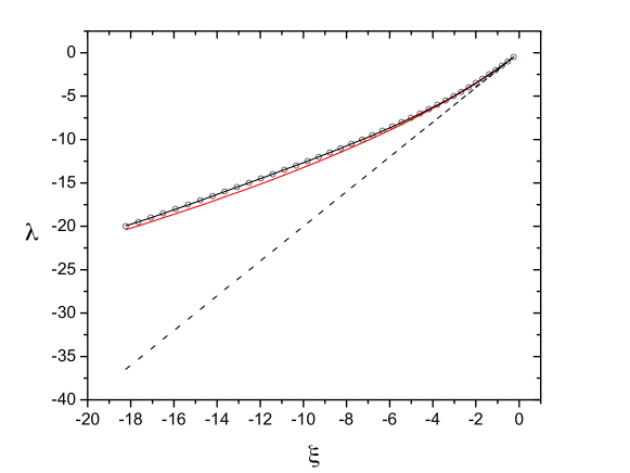
Figure 5.2: The Lagrange multiplier $\lambda$ is given as a function of the velocity gradient $\xi$. Open circles represent values obtained from the numerical solutions of Eqs. (5.15a-5.15c) (the black solid line is just a polynomial interpolation of the numerical data); red solid line: approximated instanton relation, Eq. (5.44); dashed line: $\lambda=2\xi$, which holds for asymptotically small velocity gradients.

5.2.2 The Surrogate Saddle-Point Action

The approximate instantons given by Eqs. (5.36) and (5.41) are useful for the evaluation of $I_{1}[p^{c},u^{c}]$ and $I_{2}[p^{c}]$ up to lowest non-trivial order in the functional perturbative expansion around $p^{(0)}(x,t)$. Nevertheless, they are unable to provide the observed dependence of the MSRJD action $S_{c}(\xi)$ with the velocity gradient $\xi$. In fact, $p^{(0)}(x,t)$ is proportional to $\lambda$, leading, from (5.18), to $S_{c}(\xi)=\lambda^{2}/4$, a result that is not supported by the numerical PDFs [93].

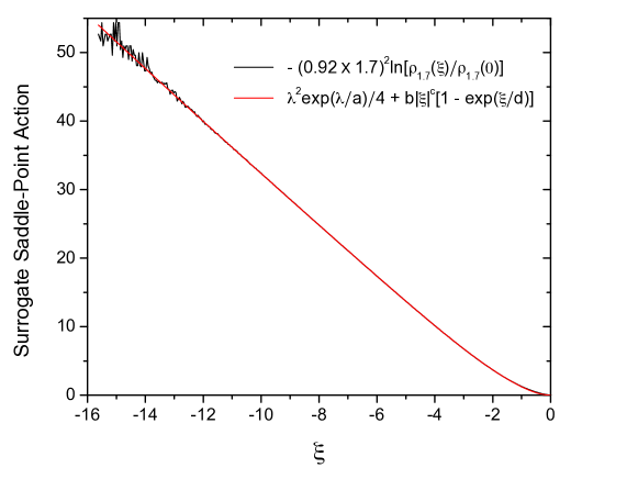
Figure 5.3: Comparison between the surrogate saddle-point action, as prescribed by [93] for the case of noise strength parameter $g=1.7$ (black solid line), and a four-parameter fitting function (red line) which provides distinct power law asymptotics for domains of small and large velocity gradients.

Taking advantage of the results reported in [93] for the case of noise strength parameter $g=1.7$, a flow regime close to the onset of intermittency, we set $\kappa(g)=(0.92)^{2}$ and write down the surrogate saddle-point action (5.32) as

$$S_{sc}(\xi)\simeq-(0.92\times 1.7)^{2}\ln\left[\frac{\rho_{1.7}(\xi)}{\rho_{1.7}(0)}\right]\ .\$$ (5.45)

To obtain the surrogate action and a set of velocity gradient PDFs for several values of $g$, direct numerical simulations were performed. They were used to check (5.20) in the approximation given by (5.22).

The stochastic Burgers equation is solved with a fully dealiased pseudo-spectral method in $N=2048$ collocation points by employing a $2^{\text{nd}}$ order predictor-corrector time evolution scheme [34, 120]. As in the numerical solution of the instanton fields, the domain size is taken to be $200L$. Velocity gradients are saved every 30 time steps after a suitable transient time, after which the total simulation time is $T\approx 1.2\times 10^{7}$.

A useful and accurate fitting of the surrogate saddle-point action (5.45) can be defined as

$$S_{sc}(\xi)=\frac{\lambda^{2}}{4}\exp\left(\frac{\lambda}{a}\right)+b|\xi|^{c}\left[1-\exp\left(\frac{\xi}{d}\right)\right]\ ,\$$ (5.46)

where $\lambda$ is given by (5.44), and $a=2.046$, $b=2.407$, $c=1.132$, and $d=2.195$ are optimal fitting parameters. This result is shown in Fig. 5.3.

The interpolation (5.46) is actually consistent with the behavior of the local stretching exponent for the saddle-point action. This exponent is defined as

$$\theta(\xi)=\frac{d\ln S(\xi)}{d\ln|\xi|}\ ,$$ (5.47)

and has been used to numerically verify the $3/2$ exponent in the asymptotic expression (5.4). At small velocity gradients, the PDF can be approximated by a Gaussian, for which $\theta(\xi)=2$, whereas at large velocity gradients the exponent transitions to $\theta(\xi)\simeq 1.16$. The expected value, on the basis of the instanton analysis [13] would be $1.5$, but high resolution numerical simulations have been unable, to this date, to observe this value. Instead, the value $1.16$ has been reported, with hints that even larger fluctuations would have to be investigated to reach the instanton scaling [91, 93]. The main benefit of using (5.46) instead of the raw surrogate saddle-point action derived from $\rho_{1.7}(\xi)$ is that it yields a smooth interpolation of data, circumventing error fluctuations that grow at larger values of $|\xi|$.

5.2.3 Evaluation of $I_{1}[p^{c},u^{c}]$ and $I_{2}[p^{c}]$

Since $I_{1}[p^{c},u^{c}]$ is a linear functional of $u^{c}(x,t)$, it can be written that, from (5.37) and (5.41):

$$\begin{split}I_{1}[p^{c},u^{c}]+I_{2}[p^{c}]&=I_{1}[p^{(0)},\lambda^{c}F_{0}^{(1)}]+\\ &+I_{1}[p^{(0)},(\lambda^{c})^{2}F_{0}^{(2)}]+I_{2}[p^{(0)}]+\mathcal{O}[\delta p^{c}]\ .\ \end{split}$$ (5.48)

In order to evaluate the first three terms on the RHS of (5.48), it is interesting, for the sake of fast numerical convergence, to write the two-point correlation functions (5.24) and (5.25) in Fourier space, viz.,

$$\tilde{G}_{pu}(k,t,t^{\prime}) =\int dx\ G_{pu}(x,0,t,t^{\prime})\exp(-ikx)$$

$$=-ig^{2}\exp\left[-(t^{\prime}-t)k^{2}\right]\Theta(t^{\prime}-t)\ ,\$$ (5.49a)

$$\tilde{G}_{uu}(k,t,t^{\prime}) =\int dx\ G_{uu}(x,0,t,t^{\prime})\exp(-ikx)$$

$$=g^{2}\sqrt{\frac{\pi}{2}}\exp\left[-\left(|t^{\prime}-t|+\frac{1}{2}\right)k^{2}\right]\ .\$$ (5.49b)

We have, from (5.27a), (5.27b), (5.49a), and (5.49b),

$$I_{1}[p^{(0)},\lambda^{c}F_{0}^{(1)}] =\frac{\lambda^{c}}{2\pi^{2}}\int_{t,t^{\prime}<0}dtdt^{\prime}\int dkdk^{\prime}~{}k(k+k^{\prime})\tilde{p}^{(0)}(k,t)\times$$

$$\times\tilde{F}_{0}^{(1)}(-k,t^{\prime})\tilde{G}_{uu}(k^{\prime},t,t^{\prime})\tilde{G}_{pu}(k+k^{\prime},t^{\prime},t)$$

$$=\frac{\lambda^{2}g^{4}}{8\pi}\int dkdk^{\prime}~{}\frac{k(k+k^{\prime})}{k^{2}+k^{\prime 2}+(k+k^{\prime})^{2}}\exp\left[-\frac{1}{2}\left(k^{2}+k^{\prime 2}\right)\right]\ ,\$$ (5.50a)

$$I_{2}[p^{(0)}] =-\frac{1}{2(2\pi)^{2}}\int_{t,t^{\prime}<0}dtdt^{\prime}\int dkdk^{\prime}\ k^{2}\times$$

$$\times\tilde{p}^{(0)}(k,t)\tilde{p}^{(0)}(-k,t^{\prime})\tilde{G}_{uu}(k^{\prime},t,t^{\prime})\tilde{G}_{uu}(k+k^{\prime},t,t^{\prime})$$

$$=-\frac{\lambda^{2}g^{4}}{16\pi}\int dkdk^{\prime}\frac{k^{2}}{k^{2}+k^{\prime 2}+(k+k^{\prime})^{2}}\exp\left[-\frac{1}{2}\left(k^{\prime 2}+(k+k^{\prime})^{2}\right)\right]\ ,\$$ (5.50b)

implying that

$$I_{1}[p^{(0)},\lambda^{c}F_{0}^{(1)}]=-I_{2}[p^{(0)}]=(3-\sqrt{3})\lambda^{2}g^{4}/24$$ (5.51)

and, according to (5.48),

$$I_{1}[p^{c},u^{c}]+I_{2}[p^{c}]=I_{1}[p^{(0)},(\lambda^{c})^{2}F_{0}^{(2)}]+\mathcal{O}[\delta p^{c}]\ .\$$ (5.52)

A straightforward numerical evaluation returns,

$$I_{1}[p^{(0)},(\lambda^{c})^{2}F_{0}^{(2)}]\simeq 1.6\times 10^{-3}\lambda^{3}g^{4}\ .\$$ (5.53)

Eqs. (5.20), (5.22), (5.26), and (5.52) provide all the ingredients needed for a perturbative analytical expression for the velocity gradient PDF:

$$\rho_{g}(\xi)=C(g)\exp\left[-\frac{1}{g^{2}}S_{sc}(\xi)+\frac{1}{2g^{4}}I_{1}[p^{(0)},(\lambda^{c})^{2}F_{0}^{(2)}]\right]\ ,\$$ (5.54)

where $C(g)$ is a normalization constant that cannot be determined from the instanton approach, since it depends on the detailed shape of the vgPDF for $-\infty<\xi<\infty$, while (5.54) refers, in principle, to negative velocity gradients which are some standard deviations away from the mean. The relevance of the saddle-point computational strategy (including fluctuations), however, can be assessed from adjustments of $C(g)$ that produce the best matches between the predicted PDFs, Eq. (5.54), and the empirical ones, obtained from the direct numerical simulations of the stochastic Burgers equation. These numerical fits are carried out in the velocity gradient range $-5g\leq\xi\leq-3g$.

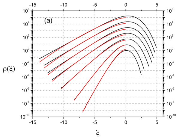
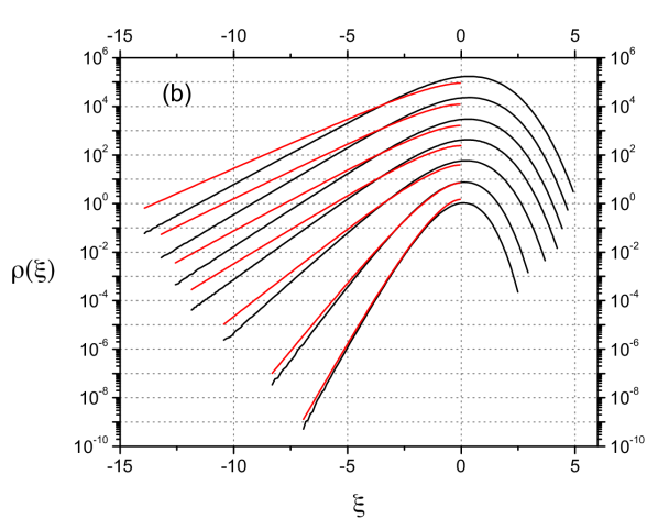
Figure 5.4: Modeled (red lines) and empirical (black lines) vgPDFs are compared for noise strengths $g=1.0,1.2,1.5,1.7,1.8,1.9$, and $2.0$. They have been shifted along the vertical axis to ease visualization, and their associated values of $g$ grow from the bottom to the top in each one of the PDF sets. Figures (a) and (b) give the modeled vgPDFs that include and neglect, respectively, the effects of fluctuations around instantons.

Comparisons between the predicted and empirical PDFs are shown in Fig. 5.4, for $g=1.0$, $1.2$, $1.5$, $1.7$, $1.8$, $1.9$, and $2.0$, with and without the fluctuation correction term proportional to $I_{1}[p^{(0)},(\lambda^{c})^{2}F_{0}^{(2)}]$, as it appears in (5.54). It can be observed in the figure that the surrogate saddle-point action is in fact a very good approximation to the exact one, by inspecting the PDF for $g=1.0$, when the cumulant contribution is almost negligible. As $g$ grows, the relative cumulant contributions grow as well, and become essential for an accurate modeling of velocity gradient PDF tails. For $g=1.7$, as an example, there is an evident intermittent left tail, with an excellent agreement between modeled and empirical PDFs that extends for about four decades.

As it can be seen from Fig. 5.4, as $g$ grows, the velocity gradient regions where the agreement between the predicted and the empirical vgPDFs is reasonably good shrink in size. This is, of course, expected under general lines, since the cumulant expansion is a perturbative method supposed to break down when the amplitude of saddle-point configurations become large enough, which in our particular case takes place for large negative velocity gradients.

5.2.4 Perturbative Domain

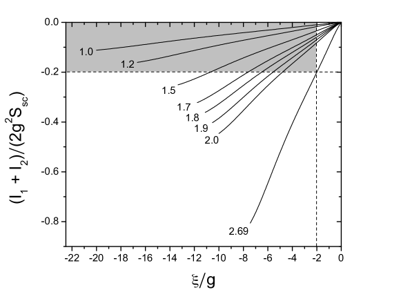
Figure 5.5: Solid lines, labeled by values of $g$, represent relative corrections to the MSRJD surrogate saddle-point action due to fluctuations around instantons. The intersection points of each one of the solid lines with the vertical and horizontal dashed lines define the range of normalized velocity gradients $\xi/g$ where the perturbative cumulant expansion is assumed to work (highlighted region in the plot).

An analysis of the results in Fig. 5.4 reveals that a fine matching between the predicted and the empirical vgPDFs holds for $|\xi|>2g$, but starts to lose accuracy when velocity gradients are such that the second order cumulant expansion contributions, $(I_{1}[p^{c},u^{c}]+I_{2}[p^{c}])/2g^{4}$, are of the order of $20\%$ (in absolute value) of the dominant saddle-point contributions, $S_{sc}(\xi)/g^{2}$. In Fig. 5.5, the ratio between these two quantities is depicted with its dependence on the velocity gradient $\xi$, for the several investigated values of the noise strength parameter $g$, up to $g=2.0$. It can be estimated in this way, then, that $g\simeq 2.7$ is an upper bound for the usefulness of the cumulant expansion method.

5.3 Discussion

The instanton approach to Burgers intermittency was introduced in [97, 13] to describe asymptotically large fluctuations, in this case, of the velocity gradient. The representation of its preasymptotic features, though, has remained obscured.

Previous results in the context of Lagrangian turbulence ([160] and [6], discussed in Chap. 4), have indicated that non-Gaussian fluctuations can be perturbatively investigated at the onset of intermittency by means of the cumulant expansion technique. The main lesson taken from these studies is that at the onset of intermittency, the MSRJD saddle-point action reaps a renormalization of its noise and heat kernels, as a dynamical effect of fluctuations around instantons. In this way, accurate comparisons between analytical and empirical velocity gradient PDFs have been achieved.

In this work, reported in [7], a similar approach has been applied to the stochastic Burgers hydrodynamics in order to predict the left tails of its velocity gradient PDF at the onset of intermittency. The results in Fig. 5.4 show that an account of fluctuations around instantons is necessary to render the instanton approach a meaningful tool for the modeling of Burgers intermittency.

Chapter 6 Shot Noise Multifractal Model for Turbulent Pseudo-Dissipation

The first observations of intermittency in turbulence were reported quite a long time ago [17] and were first addressed theoretically in [125, 169], as discussed in Sec. 2.8. In these works, scale dependent observables were postulated as the relevant quantities in the study of fluctuations in the turbulent inertial range. The theory also hypothesized that the kinetic energy dissipation, a positive quantity, follows a lognormal probability distribution, an observation which is remarkably accurate, as reported in experiments and numerical simulations [236]. Furthermore, experimental measurements of the kinetic energy dissipation revealed long-range power-law correlations [101, 185], another key feature of turbulent fields. Multifractal random fields have been a tool to describe and understand turbulent fields with such statistical properties, but their derivation on a first-principle basis is still an open problem.

The origin of the lognormal distribution of the kinetic energy dissipation has been connected to the Richardson energy cascade through several phenomenological models, beginning with discrete cascade models [168, 234, 80]. In summary, these models describe the distribution of energy dissipation across length scales in a turbulent field, from the large energy-injection scale, down to the much smaller dissipation length scales. The kinetic energy dissipation in an inviscid cascade of $n$ steps, following Eq. (2.52), can be written as a random variable

$$\varepsilon_{n}=W_{1}W_{2}\cdots W_{n}\ \varepsilon_{0}\ ,$$ (6.1)

where the $W_{i}$ are random variables which determine the energy transferred from one step to the next. For the cascade to be statistically inviscid, it is required that the $W_{i}$ are positive and have a mean value of one.

If the $W_{i}$ factors in this model are equally and independently distributed, the probability distribution for the small-scale energy dissipation is well approximated by a lognormal, since $\ln\varepsilon_{n}$ is defined as the sum of several independent random variables of finite mean and variance. The central limit theorem ensures that the probability distribution of $\ln\varepsilon_{n}$ approaches a normal distribution. As a consequence, $\varepsilon_{n}$ itself is a random variable with a lognormal distribution in the limit $n\to\infty$.

These cascade models, though, had the limitation of being discrete and of possessing a special scale ratio between neighboring scales, customarily $\lambda=2$. It was noticed in [142] that this special scale ratio should not be present, since turbulent energy dissipation displays multifractal properties for any chosen scale. Instead, a description in which arbitrary values of $\lambda$ are valid and produces multifractal statistics should be preferred and investigated, as pointed out by Mandelbrot. Furthermore, the discrete models have been able to account for scale-locality of the energy transfer process, but did not account for correlations in time. This means that such fields had no causal structure, making them difficult to connect to the dynamics of turbulent fields described by the Navier-Stokes equations. Some of these issues were addressed by the causal framework of [179], in which a stationary stochastic process is described and it is analytically verified that it satisfies the same multifractal properties as the small-scale energy pseudo-dissipation of the discrete cascade models.

This chapter describes a causal stochastic process driven by discrete and periodic random jumps, which is used to model the dynamical and multifractal properties of Lagrangian pseudo-dissipation. The observed dynamics is regular at scales below the Kolmogorov length scale, and multifractal at larger scales, demonstrating the possibility to apply discrete (shot) noise in effective models of turbulence. Our main motivation here relies on the fact that the time evolution of local Lagrangian observables is sensitive to the existence of spacetime localized perturbations of the turbulent flow, such as vortex tubes. The dynamics of spheroids in turbulent flows has been observed to be dependent on small scale properties [174, 229]. Their tumbling motion is marked by a regular evolution disrupted by intense jumps, which can be seen in Fig. 6.1, indicating that a modeling in terms of shot noise might explain their behavior. The main characteristics of a turbulent flow which lead to the preferential alignment of these spheroids is still a problem under investigation, with possible applications in industrial and natural fluid currents.

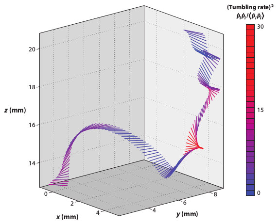
Figure 6.1: Trajectory of a rod in a turbulent flow from experiments of [174]. The color represents the tumbling rate. Figure extracted from [229].

There are infinite ways a stochastic field can be multifractal. In previous models in the literature [202, 180, 179], the lognormal description was chosen, due to its interesting statistical features (it is the simplest nontrivial continuous multifractal formulation) and to its history in connection with the statistical theory of turbulence. Furthermore, the construction of a causal equation for a multifractal field driven by shot noise requires the use of a general version of Itô’s lemma, including the contributions from discontinuities [187, 119]. This lemma and its application to the random field in case are discussed in detail.

Focusing on turbulence, it turns out, from experimental evidence [236], that several positive-definite observables like the kinetic energy dissipation, kinetic energy pseudo-dissipation, enstrophy, and the absolute value of acceleration can be reasonably well described by lognormal distributions, with a particularly good accuracy being achieved for pseudo-dissipation. In the work of Yeung and Pope, it is also remarked that the statistical moments of dissipation and enstrophy seem to approach those of the lognormal distributions as the Reynolds number increases, suggesting that further studies are required to settle this issue. Additionally, it is also known that the lognormal distribution can only be a good approximation to the statistics of dissipation, but not a complete solution which holds close to the dissipative scale or at arbitrarily high orders of the statistical moments. A discussion on consistency requirements for statistical distributions of turbulent observables can be found in [78].

6.1 Statistics of Turbulent Energy Dissipation and Pseudo-Dissipation

The first theoretical results in the statistical theory of turbulence established the picture of the turbulent cascade on a mathematical ground. This early description of Kolmogorov regards the mean behavior of the inertial range statistics of turbulent velocity fields, but not its fluctuations. Later studies of turbulent fluctuations, leading to the multifractal picture, revealed that the K41 velocity field is an exactly self-similar field of Hurst exponent $1/3$, that is, a monofractal. This field is homogeneous in space, in contrast to the complex and concentrated structures which form in isotropic flows, revealed by direct numerical simulations and experiments [107, 48, 53].

Multifractal fields have been proposed as general models to the turbulent velocity field in the inertial range, although it remains an open problem to fully characterize this multifractal field and its statistical properties. For the purpose of modeling a positive-definite scalar field, consider a generic $d$-dimensional multifractal random field $\varepsilon_{\eta}$, which may depend on the spatial variable $\bm{x}$ and on time $t$, and with a dissipative length scale $\eta$. The basic statistical properties of this random field are compatible with the features of the discrete cascade models and with experimental and numerical realizations of several observables in turbulence. The field $\varepsilon_{\eta}$ satisfies, for its statistical moments, the relation

$$\left\langle(\varepsilon_{\eta})^{q}\right\rangle=A(q)\ \eta^{K(q)}\ ,$$ (6.2)

where $A(q)$ is a $q$-dependent constant and $K(q)$ is a characteristic function of the multifractal field, connected to how structures at different scales spread across space. In particular, a lognormal distribution for $\varepsilon_{\eta}$ corresponds exactly to $K(q)=\mu q(q-1)/2$, where $\mu$ is called the intermittency parameter, which measures the intensity of the fluctuations of this field.

The variable $\varepsilon_{\eta}$ is a bare field, since it is defined at the dissipative scale. The multifractal hypothesis makes predictions for the behavior of coarse grainings of $\varepsilon_{\eta}$ as well, which are defined as local averages of the original field at the scale $\ell>\eta$, according to Eq. (2.49). In particular, the statistical moments of a coarse-grained multifractal field obey the same statistical behavior as the bare field,

$$\left\langle(\varepsilon_{\ell})^{q}\right\rangle=A^{\prime}(q)\ \ell^{K(q)}\ ,$$ (6.3)

at scales larger than the bare scale $\eta$ and up to some critical moment $q_{\mathrm{crit}}$, beyond which this scaling becomes linear [203, 135]. It is vital to know these properties for coarse-grained fields for two main reasons. First, a coarse-grained field is all experimentalists have access to. And second, the features of coarse-grained fields are a fundamental ingredient in Kolmogorov’s refined similarity hypothesis, according to which the inertial range statistical properties at scale $\ell$ depend only on $\ell$ itself and on the kinetic energy dissipation coarse-grained at this scale, $\varepsilon_{\ell}$. Thus, the verification that a given set of data does display multifractal statistics compels to the study of its coarse-grained properties.

For the general field $\varepsilon_{\eta}$, given that $X_{\eta}\equiv\ln\varepsilon_{\eta}$, its autocorrelation function decays logarithmically with the distance between the points,

$$\langle X_{\eta}(0)X_{\eta}(\bm{r})\rangle=C-\frac{\sigma^{2}}{\ln\lambda}\ln|\bm{r}|\ .$$ (6.4)

This property can be easily verified for the the discrete cascade models [9, 10, 202], in which case $\sigma^{2}=\mathrm{Var}[\ln W]$ and $C=\langle\ln W\rangle^{2}n^{2}+\sigma^{2}n$, where $n$ is the depth of the cascade and $\lambda$ the scale ratio of the model. The Fourier transform of this expression corresponds to the power spectrum, which amounts to $1/f$ noise,

$$E_{\eta}(k)\approx k^{-1}\ .$$ (6.5)

This is a common feature of intermittent fields in general and is also valid for coarse-grained fields [199, 200, 12]. The properties just presented: Eqs. (6.2), (6.3), and (6.4) are the main characteristics of a multifractal field.

To account for fluctuations into account, it was postulated by Kolmogorov and Obukhov in 1962 that the kinetic energy dissipation field follows a lognormal distribution with

$$\mathrm{Var}[\ln\varepsilon_{\ell}]=-\mu\ln(\ell/L)+C\ ,$$ (6.6)

where $L$ is the integral length scale, $\ell$ is the observation scale in the inertial range, $\eta\ll\ell\ll L$, and C is an arbitrary constant. The intermittency parameter $\mu$, the same as in the expression for $K(q)$, was historically introduced in this expression.

It was later realized [234] that the intermittency parameter is also responsible for the power-law correlations of the kinetic energy dissipation, in the form

$$\langle\varepsilon_{\eta}(\bm{r})\varepsilon_{\eta}(\bm{r+\delta r})\rangle\propto(L/\ell)^{\mu}\ ,$$ (6.7)

where $\ell\equiv|\bm{\delta r}|$ and the parameter $\mu$ is apparent as well. The cascade models were built to explain these statistical features.

The specific random fields considered in this chapter, as well as [202, 180, 179] are one-dimensional and depend only on time, since they correspond to some positive-definite observable following a Lagrangian trajectory of the flow. The Lagrangian view is connected to the space-time structure of the energy dissipation cascade: since eddies are carried by the flow, their statistical distribution is somehow influenced by the transport properties of the turbulent velocity field. And Lagrangian observables such as velocity differences and velocity gradients have been argued to display scaling and intermittent behavior, following a Lagrangian refined similarity hypothesis, in an equivalent manner to the Eulerian framework. Lagrangian velocity difference structure functions, for instance, are believed to scale as

$$\langle\big{(}\delta u_{i}(\tau)\big{)}^{n}\rangle\propto(\langle\varepsilon_{\tau}\rangle\tau)^{\xi_{n}}$$ (6.8)

in the Lagrangian inertial range, $\tau_{\eta}\ll\tau\ll T$, between the dissipative time scale $\tau_{\eta}$ and the integral time scale $T$. The coarse-grained Lagrangian kinetic energy dissipation, $\varepsilon_{\tau}$, is defined in terms of its bare counterpart, $\varepsilon_{\tau_{\eta}}$, in analogy with Eq. (2.49):

$$\varepsilon_{\tau}(t)=\frac{1}{\tau}\int_{t}^{t+\tau}dt^{\prime}\varepsilon_{\tau_{\eta}}(t^{\prime})\ .$$ (6.9)

Its average value $\langle\varepsilon_{\tau}\rangle$ is constant due to the stationarity of the turbulent flow. The dissipative time scale is determined from dimensional analysis as the Lagrangian analogue of the dissipative length scale, and is defined as $\tau_{\eta}=\eta^{2/3}\varepsilon_{0}^{-1/3}$ and the Lagrangian integral time is defined in terms of the velocity two-point autocorrelation $\rho_{L}(\tau)$, as $T=\int_{0}^{\infty}\rho_{L}(\tau)d\tau$. In the K41 framework, the scaling exponents of velocity difference structure functions grow linearly, and the equivalent relation in the Lagrangian view is that $\xi_{n}=n/2$. This can be understood with the framework of [27], which connects Lagrangian and Eulerian self-similarity. Eq. (6.8) has been numerically verified in [19, 196, 16], and it is notable that finite Reynolds effects are even more pronounced in the Lagrangian frame, making measurements even more difficult [235].

In [142], it was noticed that a random field built as the exponential of a Gaussian field,

$$\varepsilon_{\eta}\propto\exp\{\sqrt{\mu}X\}\ ,$$ (6.10)

would satisfy these properties. In this equation, the Gausian field $X$ is an Itô integral over the Wiener measure $dW(t)$, hence $\varepsilon_{\eta}$ can be seen as a continuous product of random factors. This is a straightforward, albeit nonrigorous, translation of Eq. (6.1) to the continuum, which has lognormal statistics as well. This construction was mathematically formalized in [115], and the modern understanding of such random fields has led to explicit frameworks in the Eulerian [178] and Lagrangian context [179], which approximate the known statistics of turbulent fields. Since Kahane, this continuous stochastic process with multifractal statistics is called Gaussian Multiplicative Chaos, in connection with the standard additive random process (the Wiener process). For an explanation of the origin of this nomenclature, the reader should consult the footnote in [190].

The discrete cascades display the same statistical properties as the small scale multifractal field of Eq. (6.10), but for a single scale ratio. Another critique of Mandelbrot on the discrete cascades was the absence of a space-time causal structure. The only causal connection in these models is between length scales, a relation which cannot be easily translated to a space-time distribution of turbulent structures or of energy dissipation. A step in this direction was performed in [202], with the study of a causal one-dimensional stochastic process, formulated in terms of a stochastic differential equation. In this work, analytical expressions for the statistical moments and two-point correlation functions of this process are proved, in agreement with the multifractal hypothesis and providing a continuous-in-scale extension of the discrete cascade models. This stochastic process, though, does not generate a stationary state solution, an issue which was resolved in [179].

The stochastic process of [179] for the evolution of the pseudo-dissipation field $\varphi_{P}$ is described by the following stochastic differential equation:

$$\begin{split}dX_{P}(t)&=\left[-\frac{1}{T}X_{P}(t)+\beta_{P}(t)\right]dt+\frac{1}{\sqrt{\tau_{\eta}}}dW(t)\ ,\\ \beta_{P}(t)&=-\frac{1}{2}\int_{s=-\infty}^{t}\frac{1}{\left(t-s+\tau_{\eta}\right)^{3/2}}dW(s)\ ,\end{split}$$ (6.11)

where the pseudo-dissipation $\varphi_{P}(t)$ is given by an exponential of the underlying $X_{P}(t)$ process, explicitly:

$$\varphi_{P}(t)=\frac{1}{\tau_{\eta}^{2}}\exp\left\{\sqrt{\mu}X_{P}(t)-\frac{\mu}{2}\mathbb{E}\left[X_{P}^{2}\right]\right\}\ ,$$ (6.12)

where $\mu$ is the Lagrangian intermittency exponent, $T$ is the integral time scale, $\tau_{\eta}$ the Kolmogorov dissipative time scale and $W(t)$ is a standard Wiener process. The stochastic processes $X_{P}(t)$ and $\varphi_{P}(t)$ reach a stationary state with lognormal and long-range correlated statistics, in the limit of $\tau_{\eta}\to 0$ (corresponding to infinite Reynolds number). Some of the necessary ingredients in a multifractal process which this equation illustrates are long-term memory and noise correlations, expressed through the $\beta_{P}(t)$ term, which is driven by the same random noise solution as the main equation, for $\varepsilon_{P}(t)$.

6.2 Stochastic Models of Lagrangian Pseudo-Dissipation

An alternative formulation of multiplicative chaos was done in [180], where a time-discretized causal multifractal process was introduced. This stochastic process satisfies the multifractal properties for its statistical moments and two-point autocorrelation functions, as well as its coarse-grained version, for which the multifractal statistics are verified for any continuous scale ratio (in the limit of infinite Reynolds number).

The stochastic process of [180], with a dissipative timescale $\tau_{\eta}$ and a large timescale corresponding to the integer $N=T/\tau_{\eta}$, is described by

$$X_{D}(t)=\frac{1}{\sqrt{\tau_{\eta}}}\sum_{k=0}^{N-1}(k+1)^{-1/2}\alpha_{t-k}\ ,$$ (6.13)

where $\alpha_{k}$ are independent and identically distributed Gaussian random variables of zero mean and standard deviation $\sqrt{\tau_{\eta}}$. The time, unlike in the previous examples, is only defined for integer $t$. This process also possesses long-term memory over the integral time scale, in connection with Eqs. (6.11). The multifractal process corresponding to Eq. (6.13) is likewise given by its exponential,

$$\varphi_{D}(t)=\varphi_{0}\exp\big{(}\sqrt{\mu}X_{D}(t)-\mu\mathbb{E}[X_{D}^{2}]/2\big{)}\ \mbox{,}$$ (6.14)

which has lognormal and long-range correlated statistics. Eq. (6.13) reaches a stationary state with the following multifractal properties:

1. Its moments satisfy

   $$\mathbb{E}[\varphi_{D}^{q}]=C_{q}\left(\frac{\tau_{\eta}}{T}\right)^{-K(q)}\ \mbox{,}$$ (6.15)

   with $K(q)=\mu\ q(q-1)/2$, conforming to the lognormal statistics, and $C_{q}$ is a factor which can be exactly calculated.

2. The coarse-grained moments of $\phi_{D}$ satisfy a similar relation with the same exponents:

   $$\mathbb{E}[(\varphi_{D})_{\tau}^{q}]\approx c_{q}\left(\frac{\tau}{T}\right)^{-K(q)}\ \mbox{,}$$ (6.16)

   where the coarse-grained field is defined as a moving average with a window of $\tau$:

   $$(\varphi_{D})_{\tau}(t)=\frac{1}{\tau}\sum_{k=t}^{t+\tau/\tau_{\eta}-1}\varphi_{D}(k)\ .$$ (6.17)

   Relation (6.16) is asymptotic, and is valid in the limit of $T$ going to infinity, with the ratio $\tau/T$ kept fixed. Furthermore, $q$ must be such that $K(q)<q-1$. The existence of upper and lower bounds on $c_{q}$ was demonstrated in [180], while precise values would have to be inspected numerically.

3. The autocovariance of this process, in the same limit of $T\to\infty$, converges to

   $$\mathrm{Cov}[\varphi_{D}(t),\varphi_{D}(t+\tau)]\approx-\mu\ln(\tau/T)\ \mbox{.}$$ (6.18)

Having Eqs. (6.15-6.18) in mind, a stochastic differential equation which inherits features from the continuous and discrete instances is described in this chapter. This stochastic field takes into account the small scales in a dynamic manner, such that it follows a smooth time evolution on scales below the Kolmogorov time, but still shows roughness and multifractal behavior on timescales much larger than that. This picture is inspired by the Kolmogorov phenomenology, in which dissipation can be neglected in the inertial range, while it acts in smoothing out the velocity field in the dissipative scale.

Furthermore, the refined similarity hypothesis states that, in the limit of infinite Reynolds numbers, all the statistical properties at scale $\ell$ are uniquely and universally determined by the scale itself and the mean energy dissipation rate coarse-grained at this scale, $\varepsilon_{\ell}$. By this hypothesis, it is expected that a variety of noise sources generate similar behavior in the inertial range, due to an independence on the details of the dissipative dynamics. For this reason, several large scale observables of the random field stirred by discrete noise should converge to the same quantities as fields driven by Wiener noise.

Studies of discrete noise (often called shot noise) or a mixture of discrete and continuous noise (or jump-diffusion) have been pursued in others areas of knowledge, such as financial economics [55, 44], neuronal systems [175, 194], atomic physics [81, 154], biomedicine [95] and image recognition [213].

Explicitly, consider the stochastic process given by the stationary solution of the following differential equation:

$$dX(t)=\left(-\frac{1}{T}X(t^{-})+\beta(t)\right)dt+\frac{1}{\sqrt{\tau_{\eta}}}\sum_{\tau_{\eta}\ell\leq t}\alpha_{\ell}\ \delta(t-\tau_{\eta}\ell)\ dt\ .$$ (6.19)

The first term on the RHS corresponds to a drift in a usual Langevin equation, and has the same form as the drift term in Eq. (6.11). The first contribution in this term is responsible for correlations of the $X(t)$ random field of characteristic time $T$, while the second is in charge of the multifractal correlations in the solution, with a similar role to the long-memory term present in Eqs. (6.11) and (6.13). The second term in Eq. (6.19) accounts for the discrete random jump contributions. These jumps occur at periodic intervals of length $\tau_{\eta}$ and have an intensity $\alpha_{\ell}$, which is a Gaussian random variable of zero mean and standard deviation of $\sqrt{\tau_{\eta}}$. Each value of $\ell$ corresponds to a jump instant $\ell\tau_{\eta}$, hence the sum is carried for all jump times prior to the observation time $t$.

It is also important to observe the presence of the $t^{-}$ in the first term which represents an instant infinitesimally preceding the current observation instant. In a stochastic process with jumps, this kind of care is needed, because the current state of the system (at $t$) depends on the continuous evolution up to time $t^{-}$ and on the value of a jump which may have happened exactly at the instant $t$, and therefore does not affect the previous state of the system, only its future evolution. For this reason, the state $X(t^{-})$ and a jump $\alpha_{\ell}$ happening exactly at $\ell\tau_{\eta}=t$ are completely independent events. In the traditional notation of point processes [187, 119], continuous random fields are taken to be càdlàg, a French acronym for continuous on the right and limit on the left. This denomination means that jumps occur exactly at the instant $t_{\ell}$, while the left-limit at $t_{\ell}^{-}$, is not at all influenced by the jump term. Then, for a discontinuous random field $f(t)$ with a random jump happening at $t_{\ell}$, being càdlàg is equivalent to

$$\lim_{t\to t_{\ell}^{-}}f(t)\neq f(t_{\ell})\ \ \mbox{and}\ \ \lim_{t\to t_{\ell}^{+}}f(t)=f(t_{\ell})\ .$$ (6.20)

The drift term in Eq. (6.19) contains a random contribution, $\beta(t)$, in correspondence with the long-term memory random contributions in [179]. The expression for this term is

$$\beta(t)=-\frac{1}{2}\sum_{\tau_{\eta}\ell\leq t}\ \frac{\alpha_{\ell}}{(t-\tau_{\eta}\ell+\tau_{\eta})^{3/2}}\ \mbox{,}$$ (6.21)

where the $\alpha_{\ell}$ are exactly the same as those already sampled randomly for Eq. (6.19). The sum is also carried out over all jump times up to the time $t$.

The solution to this equation can be written explicitly in terms of a particular realization of the random jumps:

$$\begin{split}X(t)&=\int_{s=t-T}^{t}\frac{e^{(s-t)/T}}{\sqrt{t-s+\tau_{\eta}}}\ \sum_{\ell}\alpha_{\ell}\ \delta(s-\tau_{\eta}\ell)\ ds\\ &+\frac{1}{\sqrt{T+\tau_{\eta}}}\int_{s=0}^{t}e^{(s-t)/T}\ \sum_{\ell}\alpha_{\ell}\ \delta(s-\tau_{\eta}\ell+T)\ ds\ ,\end{split}$$ (6.22)

where, after integrating over the delta functions,

$$\begin{split}X(t)&=\sum_{t-T<\tau_{\eta}\ell\leq t}\frac{e^{(\tau_{\eta}\ell-t)/T}}{\sqrt{t-\tau_{\eta}\ell+\tau_{\eta}}}\ \alpha_{\ell}\\ &+\frac{1}{\sqrt{T+\tau_{\eta}}}\sum_{0<\tau_{\eta}\ell\leq t}e^{(\tau_{\eta}\ell-t-T)/T}\ \alpha_{\ell-T/\tau_{\eta}}\ .\end{split}$$ (6.23)

From this solution, several analytical properties of the stationary stochastic field can be calculated and compared to the results of numerical simulations.

Still, the solution in Eq. (6.23) has only Gaussian fluctuations. In analogy to what is done in the discrete and continuous settings, the field with multifractal correlations is, in fact,

$$\varphi(t)=\varphi_{0}\ \exp\{\sqrt{\mu}X(t)-\mu\mathbb{E}[X(t^{-})^{2}]/2\}\ ,$$ (6.24)

where the mean value of this process is defined as $\varphi_{0}=1/\tau_{\eta}^{2}$, following the phenomenology of Kolmogorov [88]. The variance of the $X(t)$ process, $\mathbb{E}[X^{2}(t)]$, can be calculated from the analytical solution, Eq. (6.23):

$$\begin{split}\mathbb{E}[X^{2}(t)]&=\sum_{t-T\leq\tau_{\eta}\ell\leq t}\tau_{\eta}\frac{e^{2(\tau_{\eta}\ell-t)/T}}{t-\tau_{\eta}\ell+\tau_{\eta}}+\frac{\tau_{\eta}}{T+\tau_{\eta}}\sum_{0\leq\tau_{\eta}\ell\leq t}e^{2(\tau_{\eta}\ell-t)/T-2}\\ &+\frac{2\tau_{\eta}}{\sqrt{T+\tau_{\eta}}}\sum_{t-T\leq\ell\leq t}\frac{e^{2(\tau_{\eta}\ell-t)/T-1}}{\sqrt{t-\tau_{\eta}\ell+\tau_{\eta}}}\ ,\end{split}$$ (6.25)

thus it can be seen simply as a function of time.

Eq. (6.24) also explains the choice of periodic discrete noise with period $\tau_{\eta}$, instead of the common choice of Poisson noise with an equal characteristic time, which is often what is referred to as shot noise [155]. The variable $z=\exp{\sqrt{\mu}X}$, where $X$ is a sum of $N$ Gaussian random variables, follows a lognormal probability distribution. In the case of Poisson noise, the amplitudes of the jumps would be given by the normal distribution as well, but the number of jumps would be random, with a mean $N$, and $z$ would not follow a lognormal distribution exactly. In the limit of $N\to\infty$, though, both distributions coincide, by the central limit theorem.

As was done in [202, 179], a dynamical equation for the pseudo-dissipation itself can be obtained from the dynamical equation for $X(t)$, Eq. (6.19), and the relation between the $X$ and $\varphi$ variables, Eq. (6.24). Consider for a moment the general stochastic differential equation

$$dX(t)=F(t^{-},X(t^{-}))\ dt+\sum_{0\leq t_{\ell}\leq t}G(t^{-},X(t^{-}))\delta(t-t_{\ell})\alpha_{\ell}\ dt\ ,$$ (6.26)

where $F$ and $G$ are arbitrary functions of $t$ and $X(t)$, respectively called the drift and jump terms. This equation does not have any continuous noise term (proportional to a Wiener measure $dW(t)$), because the stochastic differential equation proposed in this work does not possess the Wiener term either. In addition, an appropriate set of initial conditions for $X(t)$ is provided. The new variable, $Y$, is obtained from the original variable through an arbitrary continuous function $f$, as

$$Y(t)=f(t,X(t))\ .$$ (6.27)

A stochastic differential equation for $Y(t)$ is obtained [187, 119] with Itô’s lemma for semimartingales, which is the appropriate expression for a change of variables in a stochastic process, equivalent to the chain rule in standard calculus. Semimartingales are generalizations of local martingales: While the latter are represented by continuous stochastic processes, such as the standard Brownian motion, the former may display discontinuous jumps, which are central to the current discussion. The solution $X(t)$ of Eq. (6.26) is thus a semimartingale.

In its semimartingale formulation, Itô’s lemma is expressed as

$$\begin{split}&Y(t)=Y(0)+\int_{0}^{t}\partial f(s^{-},X(s^{-}))/\partial s\ ds\\ &+\int_{0}^{t}f^{\prime}(s^{-},X(s^{-}))dX(s)+\frac{1}{2}\int_{0}^{t}f^{\prime\prime}(s^{-},X(s^{-}))d[X,X]^{c}(s)\\ &+\sum_{0\leq t_{\ell}\leq t}\Big{(}f(t_{\ell},X(t_{\ell}))-f(t_{\ell}^{-},X(t_{\ell}^{-}))-f^{\prime}(X(t_{\ell}^{-}))(X(t_{\ell})-X(t_{\ell}^{-}))\Big{)}\ .\end{split}$$ (6.28)

The integration interval, from $0$ to $t$, includes several jump instants, denoted by $t_{\ell}$ with an integer index $\ell$ differentiating each jump. Because of the discontinuities, it is important to prescribe that the $X(t)$ process is càdlàg, which means that terms of the form $X(s^{-})$ should be calculated as the limit

$$X(s^{-})=\lim_{t\to s^{-}}X(t)\ .$$ (6.29)

If $s$ is a jump instant, this limit does not include the contribution from the discontinuous jump, which is only accounted for in $X(s)$. Whereas if $s$ is not a jump instant, $X(s)$ and $f(s,X(s))$ are continuous at this point. The first four terms in the RHS of Eq. (6.28) are exactly equal to those in Itô’s lemma for continuous processes, with the only difference that the discontinuous jumps require a distinction between left and right limits. As in the traditional Itô’s lemma, the derivatives $f^{\prime}(t,X(t))$ and $f^{\prime\prime}(t,X(t))$ are taken with respect to $X(t)$.

The continuous quadratic variation $[X,X]^{c}(t)$ of the Wiener process is simply $t$, concluding the identification with the lemma for local martingales. In general, the quadratic variation is defined by

$$[X,X]_{t}=\lim_{\delta t\rightarrow 0}\sum_{k=1}^{n}\left(X_{t_{k}}-X_{t_{k-1}}\right)^{2}\ ,$$ (6.30)

where time has been partitioned into $n$ intervals of size $\delta t_{k}=t_{k}-t_{k-1}$ and $\delta t$ is the maximum size among these partitions [187, 119]. The continuous quadratic variation is the continuous part of Eq. (6.30). If the stochastic force is purely jump-discontinuous, as is the case in Eq. (6.19), its continuous quadratic variation is zero. Also, using Eq. (6.26), the discontinuity $X(t_{\ell})-X(t_{\ell}^{-})$ which appears in Eq. (6.28) is equal to $G(t_{\ell}^{-},X(t_{\ell}^{-}))\alpha_{\ell}$. Thus, replacing Eq. (6.26) in Eq. (6.28), one of the terms in $f^{\prime}(s^{-},X(s^{-}))dX(s)$ is canceled by $f^{\prime}(t_{\ell}^{-},X(t_{\ell}^{-}))(X(t_{\ell})-X(t_{\ell}^{-}))$. With this, Itô’s lemma for pure jump processes is obtained:

$$\begin{split}Y(t)&=Y(0)+\int_{0}^{t}\frac{\partial f}{\partial s}(s^{-})\ ds+\int_{0}^{t}f^{\prime}(X(s^{-}))F(s^{-},X(s^{-}))ds\\ &+\sum_{\ell}\Big{(}f(t_{\ell},X(t_{\ell}))-f(t_{\ell}^{-},X(t_{\ell}^{-}))\Big{)}\ .\end{split}$$ (6.31)

In differential notation, this is equivalent to

$$\begin{split}dY(t)&=\partial f/\partial t\ dt+f^{\prime}(X(t^{-}))F(t^{-},X(t^{-}))dt\\ &+\sum_{\ell}\Big{(}f(t_{\ell},X(t_{\ell}))-f(t_{\ell}^{-},X(t_{\ell}^{-}))\Big{)}\delta(t-t_{\ell})dt\ .\end{split}$$ (6.32)

At first glance, this definition may look circular, because the variable $Y$ and the variable $X$ appear simultaneously. In fact, only the initial condition for $X(t)$ is needed, which is easily converted to an initial condition for $Y(t)$. All other appearances of $X(t)$ in Eq. (6.32) are causal, referring to values of $Y(t)$ already calculated, thus $X(t)=f^{-1}(t,Y(t))$. The term $f(t_{\ell},X(t_{\ell}))$, when $t_{\ell}$ is a jump instant, needs the value of $X$ at the current instant, which is simply the left-limit at the jump instant with the random contribution added:

$$X(t_{\ell})=X(t_{\ell}^{-})+G(t_{\ell}^{-},X(t_{\ell}^{-}))\alpha_{\ell}\ .$$ (6.33)

Thus, Eq. (6.32) is an entirely self-consistent way to determine the time evolution of the random field $Y(t)$.

In the specific model considered in this work, the equation for $X(t)$ is Eq. (6.19). $X(t)$ is a stochastic process with Gaussian fluctuations and its exponential is the variable of interest, with lognormal fluctuations and long-range correlations. Through Itô’s lemma (Eq. 6.31), a stochastic differential equation for the pseudo-dissipation field is reached, $\varphi(t)=f(X(t))$, where the specific function $f$ corresponding to Eq. (6.27) depends only on $X$ and is defined by

$$f(X(t))=\varphi_{0}\ \exp\{\sqrt{\mu}X(t)-\mu\mathbb{E}[X^{2}(t^{-})]/2\}\ \mbox{.}$$ (6.34)

The equation for the pseudo-dissipation field obtained through Itô’s lemma is

$$\begin{split}&d\varphi(t)=\varphi(t^{-})\Bigg{(}-\frac{1}{T}\ln\frac{\varphi(t^{-})}{\varphi(0)}-\frac{\mu}{2T}\mathbb{E}[X^{2}(t^{-})]+\sqrt{\mu}\beta(t)\\ &-\frac{\mu}{2}\frac{\partial\mathbb{E}[X^{2}(t^{-})]/2}{\partial t}\Bigg{)}\ dt+\sum_{\ell}\Big{(}f(\varphi(\tau_{\eta}\ell))-f(\varphi(\tau_{\eta}\ell^{-}))\Big{)}\delta(t-\tau_{\eta}\ell)dt\ .\end{split}$$ (6.35)

Together with an initial condition, this stochastic process is then completely well defined. Since a long-term memory is present, it is necessary to provide $X(s)$ for $s\in]-T,0]$, corresponding to the past time-evolution of $X$. After a few integral times, the influence of the initial condition vanishes, and the process reaches a stationary state. At the jumping times, a new random jump intensity $\alpha_{\ell}$ is sampled and this updates the value of the $X$ variable as in Eq. (6.33), with

$$X(\tau_{\eta}\ell)=X(\tau_{\eta}\ell^{-})+\alpha_{\ell}/\sqrt{\tau_{\eta}}\ .$$ (6.36)

From the above expression, the pseudo-dissipation is simply obtained as $\varphi(\tau_{\eta}\ell)=f(X(\tau_{\eta}\ell))$.

6.3 Numerical Procedure

Numerical simulations were performed to verify the statistical properties of the shot noise driven process. The time evolution of Eq. (6.19) can be split in a deterministic contribution from the drift term, $(-X/T+\beta)$, and a jump term, proportional to a random jump intensity $\alpha_{\ell}$. There are sophisticated algorithms to obtain the solutions of general jump-diffusion equations, such as those illustrated in [35, 90], which provide a framework to deal with complex time dependence in the drift or diffusion coefficients, cases where the solution cannot be obtained with a straightforward stochastic Euler algorithm. Instead, the diffusion term in Eq. (6.19) does not display any time dependence, and the $\beta(t)$ term has a long-term memory, requiring a simpler algorithm in its implementation. With these considerations in mind, the Euler algorithm described in [35] was applied in the simulation of the stochastic jump process of Eq. (6.19).

The jumping times are known in advance, since they are periodic, and given simply by $(0,\tau_{\eta},2\tau_{\eta},\ldots)$. For each interval between two jumps, $((\ell-1)\tau_{\eta},\ell\tau_{\eta})$, the drift term is simulated with an Euler algorithm, which is used to calculate $X(t_{\ell}^{-})$. Then, the jump term is added, with the random sampling of a new random quantity which is added to determine $X(t_{\ell})$. To setup the initial conditions for the simulation, the jump intensities $\alpha_{\ell}$ are arbitrarily defined for a complete integral time in the interval $[-T,0]$. Eq. (6.21) depends on the whole time evolution of the system, hence a truncation in the past evolution is required. A complete integral time has been chosen since it provides accurate results in comparison with the theoretical means and standard deviations, as is detailed in the next section. The random jump intensities in this past interval are sampled exactly like the intensities in the core of the simulation, as Gaussian random variables of mean zero and standard deviation $\sqrt{\tau_{\eta}}$. The choice of $X(0)=0$ is made as well. The time necessary to reach a statistically stationary state in every simulation run is optimized by this choice of initial conditions, and is found to be less than two integral times for all simulations performed.

The above algorithm is used to build a sample path for the stochastic process in Eq. (6.19). This procedure was run for sample paths of thirty integral times in total, and three hundred sample paths were drawn for each value of $\tau_{\eta}$. Thus, an ensemble containing $9\times 10^{3}$ integral times is built for each $\tau_{\eta}$, providing the significant statistics used to verify the multifractal properties of the stationary random field.

The chosen values of $\ln(\tau_{\eta}/T)$ range from $-1.0$ to $-6.0$. The more negative values correspond to more intermittency and higher Reynolds number. The time step for the simulation was chosen to be $2\times 10^{-3}\tau_{\eta}$ and the Lagrangian intermittency parameter used is $\mu=0.3$, which was measured in Lagrangian trajectories from direct numerical simulations in [105].

Once the $X(t)$ process is calculated with this algorithm, the pseudo-dissipation $\varphi(t)$ is obtained as its exponential, from Eq. (6.34). It was verified that the mean and standard deviation of $X(t)$ follow the analytical results (Eq. 6.25) within error bars. This is particularly important for the evaluation of $\varphi$, which depends on the time periodic function $\mathbb{E}[X^{2}(t)]$. It is simpler and more precise to apply the analytical expression for this function (Eq. 6.25) than to store the previous integral times and compute standard deviations on the fly. For our results, the first five integral times were discarded, even though the observed times to reach a stationary state were always smaller than this. These results are reported in the next section.

6.4 Numerical Results

A sample trajectory of the shot noise multifractal process governed by Eq. (6.35) is depicted in Fig. 6.2, along with its mean behavior. Trajectories for this example were generated for $\ln\tau_{\eta}/T=-5.60$, which corresponds to one of the highest Reynolds numbers achieved in these simulations. For higher Reynolds numbers, even larger ensembles would be needed to display the same agreement between the empirical ensemble averages and theoretical predictions. This ensemble size is sufficient for other statistical measures, though, such as probability distributions and correlation functions, because averages can be taken over ensembles and time translated samples.

In Fig. 6.3, the same detailed range as the one of the inset of Fig. 6.2 is shown, which now contains the corresponding sample path of the $X(t)$ process, along with the empirical ensemble and theoretical means. The individual jumps are noticeable: They are equally likely to be positive or negative, and their intensity does not vary as vigorously as for the $\varphi(t)$ variable. The yellow curve is the ensemble average, and it is very close to the theoretical value for the mean of $X(t)$. The global character of this stochastic process is not shown, but it resembles a standard Gaussian process, since the small time scale and the periodicity of the jumps cannot be resolved if the observation window is closer to the integral scale, $T$.

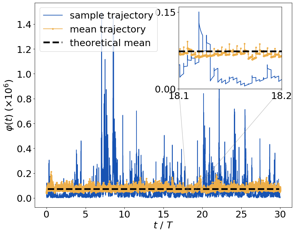
Figure 6.2: An illustration of the shot noise stochastic process for the energy pseudo-dissipation $\varphi(t)$ (Eq. 6.35). A sample path is drawn (blue), from an ensemble of three hundred paths, and shows strong and non-Gaussian fluctuations, characterized by localized large positive bursts. The ensemble mean (yellow) and the theoretical mean (black, dashed) are shown as well, and it can be seen that the numerical results accurately reproduce the correct average. In this picture, $\ln(\tau_{\eta}/T)=-5.60$. The inset shows a small stretch of the full time evolution, expanded to show details of the stochastic process at small time scales, where individual jumps can be seen. The inhomogeneity of the fluctuations can also be noticed in this smaller excerpt.

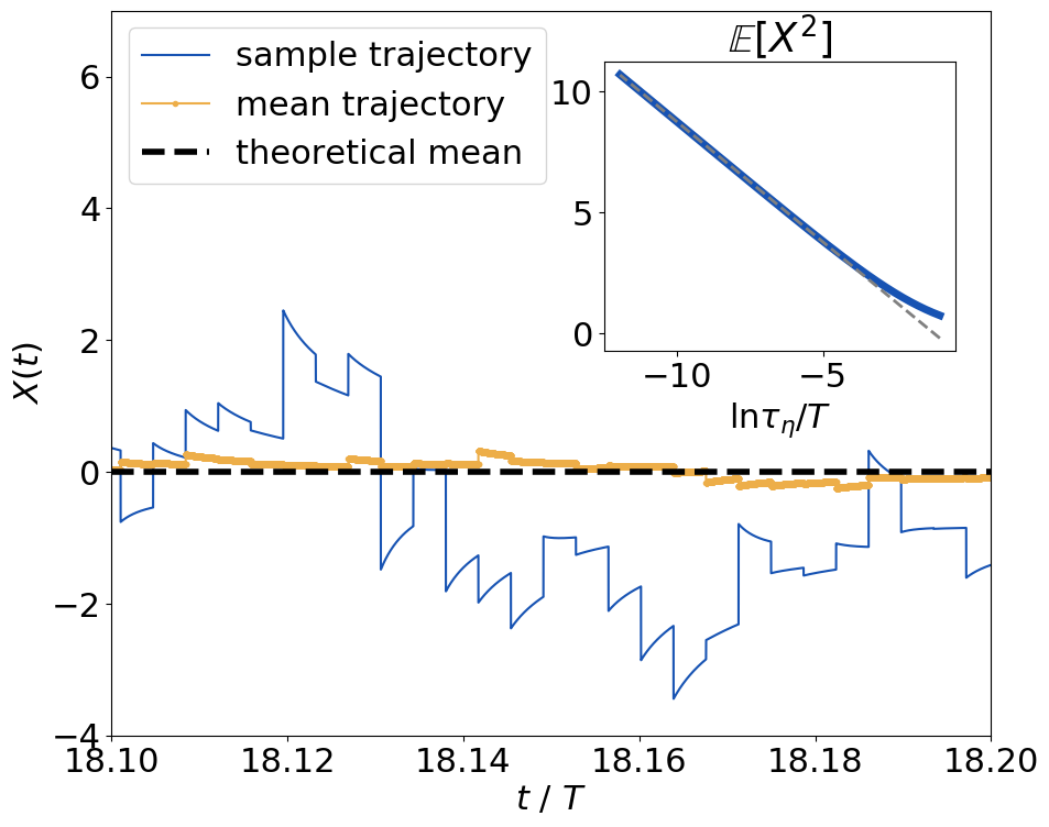
Figure 6.3: The interval depicted and the data of this figure are the same as those of the inset in Fig. 6.2. The time evolution of the stochastic Gaussian process $X(t)$ (Eq. 6.19) is shown. The individual jumps can be seen at periodic intervals of $\tau_{\eta}$, and the fluctuations are much more regular, since $X$ is a Gaussian process. The colors represent the same data as in the previous figure (with $\ln(\tau_{\eta}/T)=-5.60$): the same sample trajectory in blue, the ensemble average in yellow and the theoretical mean in black, dashed. In the inset, the variance of the process $X(t)$ is shown, with its dependence in $\ln(\tau_{\eta}/T)$. The variance is calculated analytically with Eq. (6.25) and a clear asymptotic linear behavior as $\tau_{\eta}\to 0$ is indicated by a fit in gray.

In the same figure, in the inset, the asymptotic behavior of the variance of $X(t)$ is shown. For the continuous field in [179], it was demonstrated that

$$\mathbb{E}\left[\left(X_{P}\right)^{2}\right]\underset{\tau_{\eta}\to 0}{\sim}-\ln\left(\frac{\tau_{\eta}}{T}\right)\ .$$ (6.37)

The equivalent relation for $X(t)$ is verified in Fig. 6.3. A linear fit is depicted together with the analytical curve, and the linear coefficient obtained is $0.993$. It has also been observed that this coefficient grows closer to $1.0$, the expected value for the continuous process, as the range of the fit is extended to more negative values of $\ln\tau_{\eta}/T$. This is an important property in the numerical verification that the shot noise driven process indeed displays multifractal statistics.

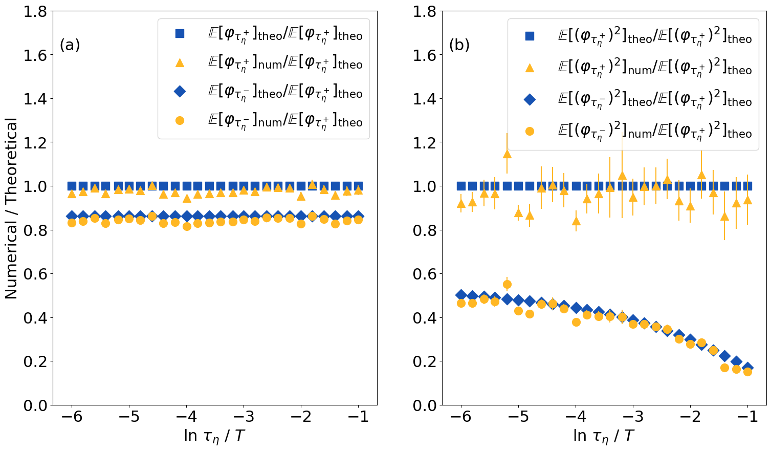
Figure 6.4: Comparison between low-order one-point statistical properties of the numerical solutions of Eq. (6.35) and their exact values. It is a consistency check on the results of the numerical calculations. The ensemble mean (a) and the variance (b) are shown. Both the mean and the variance were calculated at instants immediately before and after the jumps, and these instants are represented respectively by $\tau_{\eta}^{-}$ and $\tau_{\eta}^{+}$. Yellow symbols correspond to the numerical results, plotted with error bars in both cases, and blue corresponds to theoretical results.

Considering an instant $t$ and all other instants which differ by a multiple of $\tau_{\eta}$ from $t$, these points follow the discrete process described in [180] for different initial conditions, and its multifractal properties can be demonstrated analytically. In particular, it is obtained that

$$\mathbb{E}[\varphi^{q}(t)]_{\{t\sim t+\ell\tau_{\eta}\}}=\varphi_{0}^{q}\exp\left\{\mathbb{E}[X^{2}(t)]K(q)\right\}\ ,$$ (6.38)

in which the subscript $\{t\sim t+\ell\tau_{\eta}\}$ for the expectation value means that, in addition to the ensemble average, an average over all equivalent instants (separated by a multiple of the dissipative scale $\tau_{\eta}$) is taken as well. From this relation, taking into account Eq. (6.37), which has been verified numerically in Fig. 6.3, the multifractal dependence of the statistical moments is obtained:

$$\mathbb{E}[\varphi^{q}(t)]_{\{t\sim t+\ell\tau_{\eta}\}}=B(t)\ \varphi_{0}^{q}\left(\frac{\tau_{\eta}}{T}\right)^{-K(q)},$$ (6.39)

where $B(t)$ is a function of period $\tau_{\eta}$. The inset of Fig. 6.3, though, displays the stronger result

$$\mathbb{E}[\varphi^{q}]=\varphi_{0}^{q}\left(\frac{\tau_{\eta}}{T}\right)^{-K(q)}\ ,$$ (6.40)

where the expectation value is taken over ensemble and time translated samples. This scaling is compatible with the inset of Fig. 6.3, which shows scaling of the time average $\overline{\mathbb{E}[X^{2}(t)]}$, defined by

$$\overline{\mathbb{E}[X^{2}(t)]}=\frac{1}{\tau_{\eta}}\int_{0}^{\tau_{\eta}}\mathbb{E}[X^{2}(t)]\ dt\ ,$$ (6.41)

reason for which there is no time dependence.

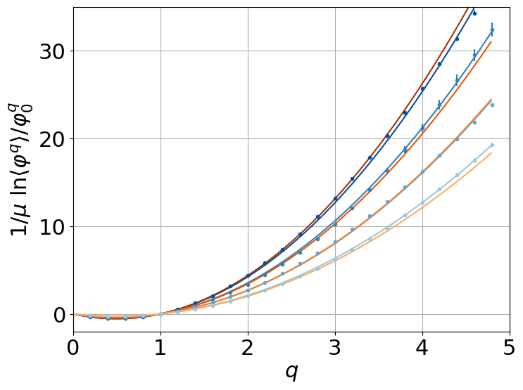
Figure 6.5: Statistical moments of the $\varphi(t)$ stochastic process, where averages are done over the ensemble and time translated samples. The numerical results correspond to the blue points, which align into a different curve for each value of $\ln\tau_{\eta}/T$, these curves are indicated in blue, calculated with a quadratic fit. All of the blue points include error bars. The values of $\ln\tau_{\eta}/T$ in this figure are $(-3.0,-3.8,-4.6,-5.6)$, with darker colors corresponding to more negative values (higher Reynolds number). In orange, quadratic theoretical curves corresponding to each of these values are displayed. The curves only deviate from each other for higher moments or higher Reynolds numbers, both regions where a significantly higher statistical ensemble would be needed.

Fig. 6.4 is a consistency test of the numerical solution of Eq. (6.35), compared with respective analytical results for the mean and variance of $\varphi(t)$ immediately before and after the jumps. In this figure, the ensemble is larger than in the previous two figures: All independent trajectories were considered, as well as all jumps in a single trajectory. In this fashion, all points immediately before (after) a jump are equivalent in order to calculate the mean and variance of $\varphi(t)$ before (after) jumps, since $\mathbb{E}[X(t)]$ and $\mathbb{E}[X^{2}(t)]$ vary periodically in time.. The points in yellow correspond to numerical averages while those in blue correspond to theoretical values, and it can be seen that, with little exceptions, the theoretical values are within the error bars of the corresponding numerical data points. Those exceptions are expected to be corrected with a larger statistical ensemble.

The statistical moments $\mathbb{E}[\varphi^{q}(t)]$ calculated from the ensemble and time translated samples, are shown in Fig. 6.5 for several values of $q$ and of $\ln\tau_{\eta}/T$. This plot verifies relation (6.40), in which all time dependence has been integrated. The numerical results, in blue points, fall in different quadratic curves according to their value of $\ln\tau_{\eta}/T$, in agreement with

$$\mathbb{E}[\varphi^{q}(t)]=\varphi_{0}^{q}\exp\left\{\overline{\mathbb{E}[X^{2}(t)]}K(q)\right\}\ ,$$ (6.42)

with $\overline{\mathbb{E}[X^{2}(t)]}$ calculated from Eqs. (6.25) and (6.41). This value is used to trace the orange theoretical curves in Fig. 6.5. The data points are well approximated by parabolic fits (blue curves) which show reasonable agreement with the theoretical expectations. Some deviation between the points and the curves are only noticeable for higher Reynolds numbers (more negative values of $\ln\tau_{\eta}/T$), represented by the darker curves, and for the higher moments. The blue curves in this figure were obtained with a fit over a quadratic function $K_{1}(q)=aq(q-1)$, and the agreement with the points and the theoretical curves is remarkable, especially for low order moments. This result is another evidence for the lognormal behavior of the jump stochastic process.

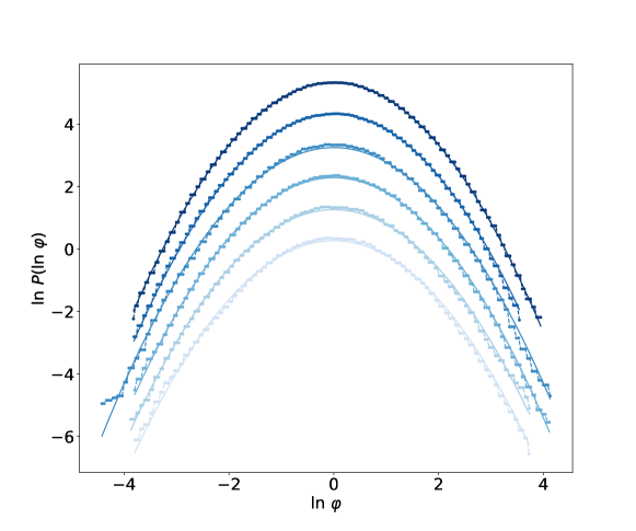
Figure 6.6: Normalized PDFs of $\ln\varphi$ are shown for the following values of $\ln\tau_{\eta}/T:(-6.0,-5.0,-4.2,-3.6,-2.8,-2.0)$, where darker colors correspond to more negative values (higher Reynolds number). The curves fall accurately on the continuous curves, which were obtained with a fit through a quadratic curve. This means that the probability distribution of pseudo-dissipation is lognormal for all values of $\tau_{\eta}$. All PDFs have been scaled to a standard Gaussian distribution (mean zero and unit variance), and they have been arbitrarily displaced upwards to simplify visualization.

Another form of visualizing the lognormal statistical distribution of the pseudo-dissipation $\varphi$ can be directly implemented from its probability distribution function. They can be seen in Fig. 6.6 for several values of $\ln\tau_{\eta}/T$. The mean and variance of the pseudo-dissipation have already been verified against their analytical results in Fig. 6.4, hence only normalized PDFs (zero mean and unit variance) are shown in Fig. 6.6. In this way, a direct comparison between the PDFs and an exact lognormal distribution can be done. The continuous curves are fits through quadratic functions, revealing that all of the curves fall closely on the expected distribution.

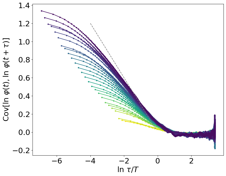
Figure 6.7: Numerical results for the autocovariance function of the pseudo-dissipation. $\tau$ is the separation between the points in this function. Colors range from yellow to purple, increasing in this order from less to more negative values of $\ln\tau_{\eta}/T$, thus the upper curves, showing a wider scaling region, are those with highest Reynolds numbers. The dashed line is the asymptotic relation for autocovariance in the continuous limit, where this function scales linearly with $\ln\tau/T$. It can be seen that as the Reynolds number grows, the region where a linear scaling can be seen grows, each curve becomes more closely linear, closer to the theoretical result for the continuous limit.

Besides their lognormal behavior, another of the most relevant features of the dissipation and pseudo-dissipation statistics is their long-range correlations, which the multifractal hypothesis is able to reproduce [100, 153, 212]. The autocovariance of the pseudo-dissipation field, $\mathrm{Cov}[\ln\varphi(t),\ln\varphi(t+\tau)]$ has been calculated to verify the existence of long-range correlations. The covariance is calculated as

$$\mathrm{Cov}[X,Y]=\mathbb{E}[(X-\langle X\rangle)(Y-\langle Y\rangle)]\ ,$$ (6.43)

and the respective numerical results can be observed in Fig. 6.7. In this figure, $\tau$ is the separation between two data points, where the range of interest lies in $\tau>\tau_{\eta}$. It can be seen that correlations grow for more negative values of $\ln\tau_{\eta}/T$, and as they grow, a larger scaling region can be seen for intermediate values of $\ln\tau/T$. This region is analogous to the inertial range in three-dimensional Navier-Stokes turbulence. In the scaling region, the autocovariance displays a dependence with $\ln\tau/T$, which is very close to linear, a relation which had been observed in [179]. This linear dependence can be understood by noticing the relation

$$\mathrm{Cov}[\ln\varphi(t),\ln\varphi(t+\tau)]=\mu\mathbb{E}[X(t)X(t+\tau)]\ ,$$ (6.44)

where a linear dependence in $\mu$ is observed. The second term, the autocorrelation of $X$, is an extension of Eq. (6.37), and in the limit $\tau_{\eta}\to 0$, it also displays a linear dependence in $\ln\tau/T$, which leads to

$$\mathrm{Cov}[\ln\varphi(t),\ln\varphi(t+\tau)]\underset{\tau_{\eta}\to 0}{\sim}-\mu\ln\left(\frac{\tau}{T}\right)\ .$$ (6.45)

The scaling region is a measure of the inertial range and is seen to grow with higher Reynolds. Also, in the gray dashed line, the exact asymptotic relation for the continuous multifractal field, Eq. (6.45), is shown, and it can be observed that the stochastic process with discrete jumps approaches the continuous limit as the intervals between jumps become smaller.

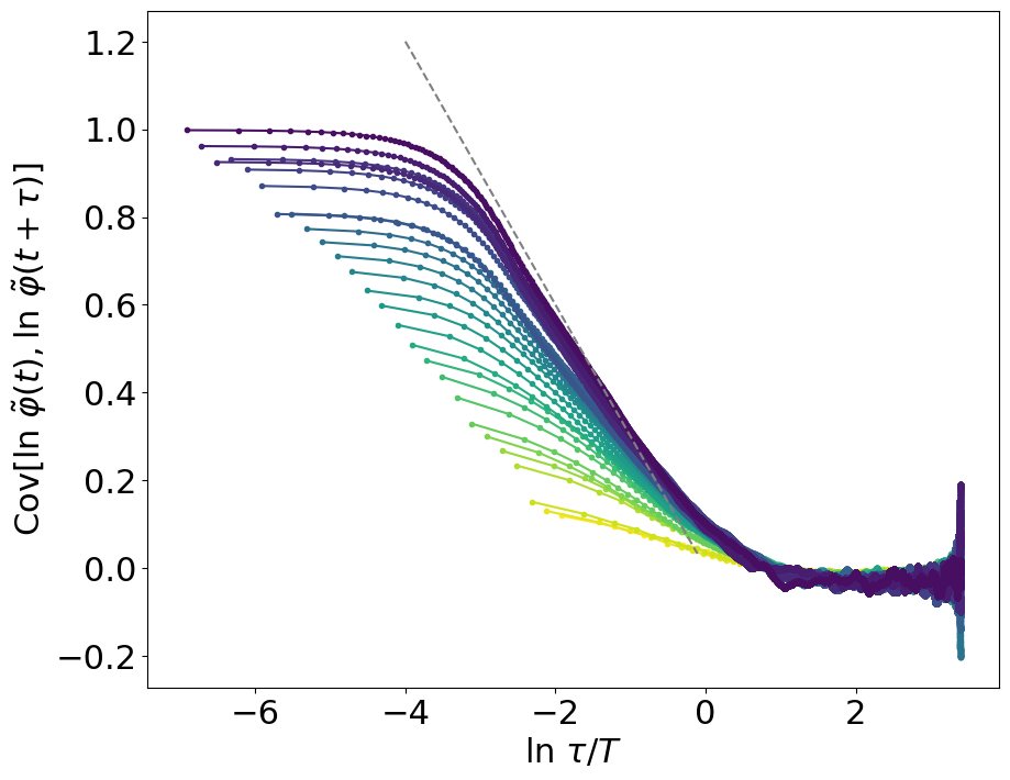
Figure 6.8: Autocovariance of the coarse-grained field $\tilde{\varphi}(t)$, in this figure the local averaging is done over a scale $\tau_{\eta}/2$. A clear scaling range, which is much more linear, can be seen in all of the curves, becoming more pronounced as the Reynolds number grows. Also, the slope of these linear curves is much closer to the theoretical value for the continuous limit, which is shown exactly the same as in the previous figure.

These statistical properties were also investigated for time averaged fields, denoted by $\tilde{\varphi}(t)$ and calculated as

$$\tilde{\varphi}(t)=\frac{1}{\tau}\int_{t}^{t+\tau}\varphi(t^{\prime})\ dt^{\prime}\ ,$$ (6.46)

where $\tau$ is the averaging scale under consideration. This observable is inspired by the hypothesis of refined similarity in the Lagrangian context as discussed in Section 6.1. The one point statistical measures (namely PDF and statistical moments, in Figs. 6.5 and 6.6) of coarse grained fields did not show appreciable difference from their fine grained versions, and for this reason the corresponding figures are not shown. Yet for the autocovariance, which is a two point statistical observable, a different behavior for the coarse-grained field is noticed, still compatible with the asymptotic description of the continuous field. In Fig. 6.8, the autocovariance of the coarse-grained fields is seen, and the linear behavior observed in Fig. 6.7 for the fine-grained covariance is revealed to be even more pronounced: The inertial range is more clearly visible, and grows as $\tau_{\eta}\to 0$, and its slope closely approaches the theoretical value in the continuous limit.

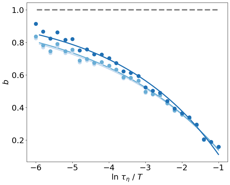
Figure 6.9: Each point has been obtained from a numerical fit of the inertial range of the autocovariance, according to Eq. (6.47). In this range, the asymptotic scaling Eq. (6.47) is valid. Each color corresponds to a different coarse-graining scale, where the values shown are $\tau=(\tau_{\eta}/3,\tau_{\eta}/2,\tau_{\eta})$, higher values are represented in darker colors. An exponential fit, with Eq. (6.48), through these numerical values was done to demonstrate the tendency of the data to approach the value $b=1$. This exponential fit is shown in the continuous curves. The gray dashed line on the top corresponds to $b=1$, indicating the high Reynolds number limit.

In order to investigate the convergence to the continuous limit, the autocovariance in the inertial range was fitted to an asymptotic functional form linear in $\ln\tau/T$ with a free parameter:

$$\mathrm{Cov}[\ln\tilde{\varphi}(t),\ln\tilde{\varphi}(t+\tau)]=-b\mu\ln\tau/T\ .$$ (6.47)

The constant $b$ is a measure of the rate of convergence to the asymptotic continuous behavior, where $b=1$. The evolution of this parameter as the dissipative scale $\tau_{\eta}$ changes can be seen in Fig. 6.9, where the points correspond to numerical fits over the respective inertial ranges. Each color represents a different coarse-graining scale $\tau$ in Eq. (6.46), and as this scale grows, convergence to the continuous becomes faster. This property was observed in the autocovariance, in Fig. 6.8, and is verified in Fig. 6.9.

Further evidence of the accelerated convergence produced by coarse-graining was obtained with a numerical fit of the curves in Fig. 6.9. These points slowly approach the asymptotic continuous value, $b=1$, and an exponential fit can make this argument quantitative. The function

$$\chi(\tau_{\eta})=1+\alpha\exp(\beta\ln\tau_{\eta}/T)$$ (6.48)

approaches 1 as $\tau_{\eta}\to 0$, and is represented in the figure in continuous curves. The curves serve as a guide to the eye on the evolution of the slope $b$ as the Reynolds number grows, and furthermore show that for the higher values of $\tau$, this convergence is hastened. The exponential shape is only a plausible approximation to a curve which asymptotically approaches a value, hence fluctuations around this curve can be seen in the data. Furthermore, the inertial range is narrow for values of $\ln\tau_{\eta}/T$ closer to zero, which make the fit more delicate in this region. It can also be observed from Fig. 6.9 that an increase of a few percent in the value of $b$ (Eq. 6.47) would require the smallest $\tau_{\eta}$ to be one or two orders of magnitude lower, corresponding to a significant increase in computational effort.

6.5 Discussion

Positive-definite quantities such as dissipation, pseudo-dissipation and enstrophy have been observed to display nearly lognormal probability distributions and long-range correlations [236], and such statistical properties can be understood under the multifractal formulation of turbulent flows, leading to a connection between the statistics and the geometrical properties of the energy cascade.

The stochastic process driven by shot noise discussed in this chapter was verified to display multifractal properties, particularly a lognormal distribution and a power-law long-range correlation. These properties have been verified for fine and coarse grained fields, which is an important feature in the application of such models to real world Lagrangian trajectories.

Chapter 7 Conclusion

In this dissertation, two main approaches to the theoretical description of large fluctuations in turbulence have been pursued: functional methods and the modelling through non-Markovian stochastic processes, with techniques coming from statistical field theory, random fields, statistical analysis and numerical methods. In this closing chapter, the main results of each previous chapter and directions for further research are laid out.

In Chap. 4, an analytical technique for the description of PDF cores of non-gaussian observables is described and applied to the RFD model of Lagrangian turbulence. This analysis verified the accuracy of the analytical instanton approximation and determined a hierarchical ordering of the perturbative diagrams according to their relevance. The same technique was also applied to the Burgers model in Chap. 5, and it was revealed that a provisional noise renormalization procedure, previously observed on the velocity gradient PDFs can be explained as the product of fluctuations around the asymptotic instanton description.

Further questions remain on these matters, nevertheless. Numerical (exact) instantons could generate results of higher precision and a broader regime of validity to the studies of [6, 7]. The exact instantons have been studied in [92, 96, 56], but not the contribution from their fluctuations. This analytical approach permits the study of complex statistical observables such as conditional measures without the need to generate huge ensembles for the measurement of the frequency of intense fluctuations.

In the stochastic Burgers model, the negative velocity gradient asymptotic exponent of $3/2$ (Eq. 5.4), although obtained as a theoretical result in [13], has so far not been observed in numerical simulations of this system, instead the value of $1.16$ is reported [93]. The investigation of the influence of noise in this problem, though, requires non perturbative techniques to describe the preasymptotic tails of the negative velocity gradient probability distribution.

Further applications of the functional methods described are also possible. For instance, the investigation of circulation statistics in three or two-dimensional Navier-Stokes turbulence [157, 208, 70], or the transport of passive scalars [14].

The work of Chap. 6 adds to the effort of building a causal structure to continuous and scale invariant energy cascades. This is done through the modeling of the Lagrangian pseudo-dissipation with a multifractal random field driven by periodic shot noise, which is found to be lognormal and long-range correlated. Nevertheless, futher investigation is required to verify from DNS the statistical properties of Lagrangian dissipation and pseudo-dissipation, in order to understand how well such models represent real energy cascades. In this investigation, understanding the behavior of coarse-grained cascades is crucial, as discussed.

The understanding of Lagrangian fluctuations is key to the effective modeling of transport properties, either of particles or fields, and to the understanding of the motion of extended structures in turbulence, such as filaments, rods and surfaces. They are heavily influenced by the localized intense bursts of energy dissipation, but still poorly understood theoretically.

Appendix A Computation Resources

Some of the computational tools developed during the work on this thesis might be of interest to other students, and the purpose of this section is to share these tools. The tool below was built with the Mathematica software and its code is freely available on Github, with a short link provided.

A.1 Tensor Contraction

This program performs contraction of indices on Euclidean tensors written with the Einstein summation convention. There already are specific packages for tensor manipulations, especially in the context of General Relativity, but they provide more general functionality at the expense of a more complex interface. In the context of the RFD model (Chapter 4), only manipulations of Euclidean tensors are necessary, a case in which there is no difference between covariant and contravariant indices.

The function contract was built in order to carry out tensor contractions in arbitrarily long products of Euclidean tensors. For instance, consider the isotropic tensor $G_{ijkl}$ defined in Eq. (4.7):

$$G_{ijkl}=2\delta_{ik}\delta_{jl}-\frac{1}{2}\delta_{il}\delta_{jk}-\frac{1}{2}\delta_{ij}\delta_{kl}\ .$$ (A.1)

The diagrammatic contributions of Eqs. (4.52) and (4.54) are obtained as specific contractions of products of this tensor. As a demonstration of this function, some results are shown in Fig. A.1, corresponding to the following operations: $G_{ikil}$, $G_{iijj}$, $G_{ijij}$ and $G_{ijkl}G_{klmn}$.

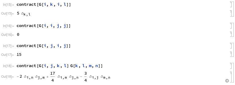
Figure A.1: A picture from the Mathematica software, with examples of tensor contractions performed with the contract function on the tensor $G_{ijkl}$.

As another example, the specific contraction which produces the result of Eq. (4.52) is depicted in Fig. A.2.

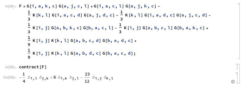
Figure A.2: Tensor contraction for the noise renormalization in the RFD model.

As a last example, contractions of the tensor $G_{ijkl}$ with arbitrary vectors, denoted by $u$ and $v$, are shown, in Fig. A.3.

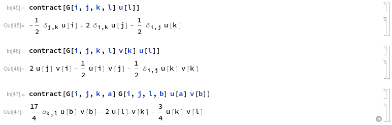
Figure A.3: Tensor contractions including products of tensors and vectors.

A final remark is that this function can only perform contractions of repeated indices, while the value of individual elements of a tensor should be obtained manually, or with other tools.

The code for the contract function is available at https://git.io/fjQe8.

Appendix B Cumulant Expansion

The cumulant expansion is a standard technique in statistics which is used to approximate a distribution or expectated value. They can be used as a simple way to describe the differences between a distribution and its Gaussian approximation. In quantum field theory, in particular, it is often necessary to compute $\langle e^{x}\rangle$, and the cumulant expansion offers a systematic way to obtain this result perturbatively in terms of the moments of the random variable $x$, which are $\langle x^{p}\rangle$.

This particular derivation is carried out to order $O(x^{3})$, but it can be extended without further complications to arbitrary order. It is interesting to notice that there is no general way to obtain the coefficients of the cumulant expansion, other than following an algorithm, be it the one below or an equivalent.

To begin with, an expansion of the exponential produces

$$\begin{split}\langle e^{x}\rangle&=\left\langle 1+x+\frac{x^{2}}{2!}+O(x^{3})\right\rangle\\ &=1+\langle x\rangle+\frac{\langle x^{2}\rangle}{2}+O(x^{3})\ .\end{split}$$ (B.1)

Taking the logarithm of both sides and a further series expansion, the following result is obtained:

$$\begin{split}\ln\langle e^{x}\rangle&=\ln\left(1+\langle x\rangle+\frac{\langle x^{2}\rangle}{2}+O(x^{3})\right)\\ &=\langle x\rangle+\frac{\langle x^{2}\rangle}{2}-\frac{\langle x\rangle^{2}}{2}+O(x^{3})\ .\end{split}$$ (B.2)

The desired result is then achieved as an exponential of the previous result,

$$\langle e^{x}\rangle\simeq\exp\left\{\langle x\rangle+\frac{1}{2}\big{(}\langle x^{2}\rangle-\langle x\rangle^{2}\big{)}+O(x^{3})\right\}\ .$$ (B.3)

By dropping the error term, this is a pragmatic way to perturbatively evaluate the given expected value.

Further references on cumulants can be found in [148, 167], and a list of coefficients for expansions of high order is provided as sequence A127671 of the Online Encyclopedia of Integer Sequences (OEIS), available in [170].

Bibliography

- [1] M.. Afonso and C. Meneveau “Recent fluid deformation closure for velocity gradient tensor dynamics in turbulence: Timescale effects and expansions” In Physica D 239 Elsevier, 2010, pp. 1241–1250
- [2] AMERICAN INSTITUTE OF PHYSICS “Jean Perrin” https://history.aip.org/phn/11807006.html [Accessed: February 24th, 2020], 2019
- [3] D.. Amit and V. Martin-Mayor “Field theory, the renormalization group, and critical phenomena: Graphs to computers” World Scientific Publishing Company, 2005
- [4] F. Anselmet, Y. Gagne, E.. Hopfinger and R.. Antonia “High-order velocity structure functions in turbulent shear flows” In J. Fluid Mech. 140 Cambridge University Press, 1984, pp. 63–89
- [5] G.. Apolinário and L. Moriconi “Shot noise multifractal model for turbulent pseudo-dissipation” In J. Stat. Mech. 2020 IOP Publishing, 2020, pp. 073208
- [6] G.. Apolinário, L. Moriconi and R.. Pereira “Instantons and fluctuations in a Lagrangian model of turbulence” In Physica A 514 Elsevier, 2019, pp. 741–757
- [7] G.. Apolinário, L. Moriconi and R.. Pereira “Onset of intermittency in stochastic Burgers hydrodynamics” In Phys. Rev. E 99 APS, 2019, pp. 033104
- [8] Z.. Arenas and D.. Barci “Functional integral approach for multiplicative stochastic processes” In Phys. Rev. E 81 APS, 2010, pp. 051113
- [9] A. Arneodo, E. Bacry, S. Manneville and J.-F. Muzy “Analysis of random cascades using space-scale correlation functions” In Phys. Rev. Lett. 80 APS, 1998, pp. 708
- [10] A. Arneodo, E. Bacry and J.-F. Muzy “Random cascades on wavelet dyadic trees” In J. Math. Phys 39 AIP, 1998, pp. 4142–4164
- [11] L. Bachelier “Théorie de la spéculation” In Annales scientifiques de l’École normale supérieure 17, 1900, pp. 21–86
- [12] E. Bacry, J. Delour and J.-F. Muzy “Multifractal random walk” In Phys. Rev. E 64 APS, 2001, pp. 026103
- [13] E. Balkovsky, G. Falkovich, I. Kolokolov and V. Lebedev “Intermittency of Burgers’ turbulence” In Phys. Rev. Lett. 78 APS, 1997, pp. 1452
- [14] E. Balkovsky and V. Lebedev “Instanton for the Kraichnan passive scalar problem” In Phys. Rev. E 58 APS, 1998, pp. 5776
- [15] P. Ball “The Scientific Problem That Must Be Experienced” http://nautil.us/issue/15/turbulence/the-scientific-problem-that-must-be-experienced [Accessed: February 24th, 2020], 2014
- [16] M. Barjona and C.. Silva “Kolmogorov’s Lagrangian similarity law revisited” In Phys. Fluids 29 AIP Publishing LLC, 2017, pp. 105106
- [17] G.. Batchelor and A.. Townsend “The nature of turbulent motion at large wave-numbers” In P. Roy. Soc. Lond. A Mat. 199, 1949, pp. 238–255
- [18] A.. Belavin, A.. Polyakov, A.. Schwartz and Y.. Tyupkin “Pseudoparticle solutions of the Yang-Mills equations” In Phys. Lett. B 59, 1975, pp. 85–87
- [19] R. Benzi et al. “Velocity-gradient statistics along particle trajectories in turbulent flows: The refined similarity hypothesis in the Lagrangian frame” In Phys. Rev. E 80 APS, 2009, pp. 066318
- [20] R. Benzi et al. “Inertial range Eulerian and Lagrangian statistics from numerical simulations of isotropic turbulence” In J. Fluid Mech. 653 Cambridge University Press, 2010
- [21] R. Benzi, B. Legras, G. Parisi and R. Scardovelli “Conformal field theory and direct numerical simulation of two-dimensional turbulence” In Europhys. Lett.) 29 IOP Publishing, 1995, pp. 203
- [22] A. Berera and R…. Ho “Chaotic properties of a turbulent isotropic fluid” In Phys. Rev. Lett. 120 APS, 2018, pp. 024101
- [23] D. Bernard “Turbulence for (and by) amateurs”, 2020 arXiv:cond-mat/0007106
- [24] D. Bernard and K. Gawedzki “Scaling and exotic regimes in decaying Burgers turbulence” In J. Phys. A 31 IOP Publishing, 1998, pp. 8735
- [25] G. Boffetta and S. Musacchio “Chaos and predictability of homogeneous-isotropic turbulence” In Phys. Rev. Lett. 119 APS, 2017, pp. 054102
- [26] G. Boffetta and I.. Sokolov “Relative dispersion in fully developed turbulence: the Richardson’s law and intermittency corrections” In Phys. Rev. Lett. 88 APS, 2002, pp. 094501
- [27] M.. Borgas “The multifractal Lagrangian nature of turbulence” In Philos. T. Roy. Soc. A 342 The Royal Society London, 1993, pp. 379–411
- [28] M. Bourgoin et al. “The role of pair dispersion in turbulent flow” In Science 311 American Association for the Advancement of Science, 2006, pp. 835–838
- [29] R. Brown “Mikroskopische Beobachtungen über die im Pollen der Pflanzen enthaltenen Partikeln, und über das allgemeine Vorkommen activer Molecüle in organischen und unorganischen Körpern” In Ann. Phys. 90 Wiley Online Library, 1828, pp. 294–313
- [30] J.. Burgers “A mathematical model illustrating the theory of turbulence” In Adv. Appl. Mech. 1, 1948
- [31] O. Cadot et al. “Energy injection in closed turbulent flows: Stirring through boundary layers versus inertial stirring” In Phys. Rev. E 56 APS, 1997, pp. 427
- [32] L. Canet “Time dependence of correlation functions in homogeneous and isotropic turbulence” http://www.nctr.eu/images/2019/lectures/Lecture_Canet_NCTRV.pdf [Accessed: February 24th, 2020], Lecture notes, 2019
- [33] L. Canet, B. Delamotte and N. Wschebor “Fully developed isotropic turbulence: Nonperturbative renormalization group formalism and fixed-point solution” In Phys. Rev. E 93 APS, 2016, pp. 063101
- [34] C. Canuto, M.. Hussaini, A. Quarteroni and A. Thomas Jr “Spectral methods in fluid dynamics” Springer Science & Business Media, 2012
- [35] B. Casella and G.. Roberts “Exact simulation of jump-diffusion processes with Monte Carlo applications” In Methodol. Comput. Appl. 13 Springer, 2011, pp. 449–473
- [36] A.. Chernykh and M.. Stepanov “Large negative velocity gradients in Burgers turbulence” In Phys. Rev. E 64 APS, 2001, pp. 026306
- [37] M. Chertkov, A. Pumir and B.. Shraiman “Lagrangian tetrad dynamics and the phenomenology of turbulence” In Phys. Fluids, 1999, pp. 2394
- [38] L. Chevillard, B. Castaing, E. Lévêque and A. Arneodo “Unified multifractal description of velocity increments statistics in turbulence: Intermittency and skewness” In Physica D 218, 2006, pp. 77
- [39] L. Chevillard and C. Meneveau “Lagrangian dynamics and statistical geometric structure of turbulence” In Phys. Rev. Lett. 97, 2006, pp. 174501
- [40] D. Chowdhury, L. Santen and A. Schadschneider “Statistical physics of vehicular traffic and some related systems” In Phys. Rep. 329 Elsevier, 2000, pp. 199–329
- [41] S. Coleman “Aspects of symmetry” Cambridge University Press, 1988
- [42] P. Constantin, W. E and E.. Titi “Onsager’s conjecture on the energy conservation for solutions of Euler’s equation” In Commun. Math. Phys. 165 Springer, 1994, pp. 207–209
- [43] I.. Cornfeld, S.. Fomin and Y.. Sinai “Ergodic theory” Springer Science & Business Media, 2012
- [44] S.. Das “The surprise element: jumps in interest rates” In J. Econometrics 106 Elsevier, 2002, pp. 27–65
- [45] C. De Lellis and L. Székelyhidi “The Euler equations as a differential inclusion” In arXiv preprint math/0702079, 2007
- [46] C. De Lellis and L. Székelyhidi “On turbulence and geometry: from Nash to Onsager” In arXiv preprint arXiv:1901.02318, 2019
- [47] P. Debue et al. “Experimental test of the crossover between the inertial and the dissipative range in a turbulent swirling flow” In Phys. Rev. Fluids 3 APS, 2018, pp. 024602
- [48] P. Debue et al. “Experimental test of the crossover between the inertial and the dissipative range in a turbulent swirling flow” In Phys. Rev. Fluids 3 APS, 2018, pp. 024602
- [49] C. Denniston and M.. Robbins “General continuum boundary conditions for miscible binary fluids from molecular dynamics simulations” In J. Chem. Phys. 125 American Institute of Physics, 2006, pp. 214102
- [50] A. Dewan “Tackling turbulent flows in engineering” Springer Science & Business Media, 2010
- [51] C. Dominicis “Techniques de Renormalization de la Theorie des Champs et Dynamique des Phenomenes Critques” In J. Phys. Colloques 37, 1976, pp. 247
- [52] H.. Dryden “A review of the statistical theory of turbulence” In Q. Appl. Math. 1, 1943, pp. 7–42
- [53] B. Dubrulle “Beyond Kolmogorov cascades” In J. Fluid Mech. 867 Cambridge University Press, 2019
- [54] J. Duchon and R. Robert “Inertial energy dissipation for weak solutions of incompressible Euler and Navier-Stokes equations” In Nonlinearity 13 IOP Publishing, 2000, pp. 249
- [55] D. Duffie, J. Pan and K. Singleton “Transform analysis and asset pricing for affine jump-diffusions” In Econometrica 68 Wiley Online Library, 2000, pp. 1343–1376
- [56] L. Ebener et al. “Instanton based importance sampling for rare events in stochastic PDEs” In Chaos 29 AIP Publishing, 2019, pp. 063102
- [57] M. Eckert “A kind of boundary-layer “flutter”: The turbulent history of a fluid mechanical instability” In arXiv preprint arXiv:1706.00334, 2017
- [58] A. Einstein “On the movement of small particles suspended in station- ary liquid demanded by the molecular-kinetic theory of heat” In Ann. Phys.-Leipzig 31, 1905, pp. 132
- [59] R.. Ellis “Entropy, large deviations, and statistical mechanics” Springer, 2007
- [60] ENGINEERING TOOLBOX “Air - Dynamic and Kinematic Viscosity ” https://www.engineeringtoolbox.com/air-absolute-kinematic-viscosity-d_601.html [Accessed: February 24th, 2020], 2003
- [61] ENGINEERING TOOLBOX “Water - Dynamic and Kinematic Viscosity” https://www.engineeringtoolbox.com/water-dynamic-kinematic-viscosity-d_596.html [Accessed: February 24th, 2020], 2004
- [62] L.. Evans “An introduction to stochastic differential equations” American Mathematical Soc., 2012
- [63] G.. Eyink “Turbulence Theory: Course Notes” http://www.ams.jhu.edu/~eyink/Turbulence/notes.html [Accessed: February 24th, 2020], 2008
- [64] G.. Eyink “Stochastic flux freezing and magnetic dynamo” In Phys. Rev. E 83 APS, 2011, pp. 056405
- [65] G.. Eyink and K.. Sreenivasan “Onsager and the theory of hydrodynamic turbulence” In Rev. Mod. Phys. 78 APS, 2006, pp. 87
- [66] G. Falkovich, K. Gawedzki and M. Vergassola “Particles and fields in fluid turbulence” In Rev. Mod. Phys. 73 APS, 2001, pp. 913
- [67] G. Falkovich and A. Hanany “Is 2D turbulence a conformal turbulence?” In Phys. Rev. Lett. 71 APS, 1993, pp. 3454
- [68] G. Falkovich, I. Kolokolov, V. Lebedev and A. Migdal “Instantons and intermittency” In Phys. Rev. E 54 APS, 1996, pp. 4896
- [69] G. Falkovich and V. Lebedev “Universal direct cascade in two-dimensional turbulence” In Phys. Rev. E 50 APS, 1994, pp. 3883
- [70] G. Falkovich and V. Lebedev “Vorticity statistics in the direct cascade of two-dimensional turbulence” In Phys. Rev. E 83 APS, 2011, pp. 045301
- [71] M. Farge “Wavelet transforms and their applications to turbulence” In Annu. Rev. Fluid Mech. 24 Annual reviews 4139 El Camino Way, PO Box 10139, Palo Alto, CA 94303-0139, USA, 1992, pp. 395–458
- [72] C.. Fefferman “Existence and smoothness of the Navier-Stokes equation” In The Millennium Prize Problems 57 Clay Math. Inst. Cambridge, MA, 2006, pp. 67
- [73] R.. Feynman “Statistical Mechanics, A set of lectures” In Frontiers in Physics. Perseus Books, 1972
- [74] R.. Feynman, R.. Leighton and M. Sands “The Feynman Lectures on Physics” Basic books, 2011
- [75] C. Foias, O. Manley, R. Rosa and R. Temam “Navier-Stokes equations and turbulence” Cambridge University Press, 2001
- [76] D. Forster, D.. Nelson and M.. Stephen “Large-distance and long-time properties of a randomly stirred fluid” In Phys. Rev. A 16 APS, 1977, pp. 732
- [77] U. Frisch “From global scaling, a la Kolmogorov, to local multifractal scaling in fully developed turbulence” In P. Roy. Soc. Lond. A Mat. 434 The Royal Society London, 1991, pp. 89–99
- [78] U. Frisch “Turbulence: The legacy of A. N. Kolmogorov” Cambridge University Press, 1995
- [79] U. Frisch and G. Parisi “On the singularity structure of fully developed turbulence” In Turbulence and predictability in geophysical fluid dynamics and climate dynamics, 1985
- [80] U. Frisch, P.-L. Sulem and M. Nelkin “A simple dynamical model of intermittent fully developed turbulence” In J. Fluid Mech. 87 Cambridge University Press, 1978, pp. 719–736
- [81] K. Funke “Jump relaxation in solid electrolytes” In Prog. Solid State Ch. 22 Elsevier, 1993, pp. 111–195
- [82] A.. Fursikov and M.. Vishik “Mathematical problems of statistical hydrodynamics” Kluwer Academic Publisher, Dordrecht, 1988
- [83] H. Furstenberg “The structure of distal flows” In Am. J. Math. 85 JSTOR, 1963, pp. 477–515
- [84] B. Galanti and A. Tsinober “Is turbulence ergodic?” In Phys. Lett. A 330 Elsevier, 2004, pp. 173–180
- [85] C. Gardiner “Stochastic methods”, 2009
- [86] K. Gawedzki “Soluble models of turbulent advection” In arXiv preprint nlin/0207058, 2002
- [87] K. Gawedzki and M. Vergassola “Phase transition in the passive scalar advection” In Physica D 138 Elsevier, 2000, pp. 63–90
- [88] S.. Girimaji and S.. Pope “A diffusion model for velocity gradients in turbulence” In Phys. Fluids A 2 AIP, 1990, pp. 242–256
- [89] S.. Girimaji and S.. Pope “Material-element deformation in isotropic turbulence” In J. Fluid Mech. 220 Cambridge University Press, 1990, pp. 427–458
- [90] F.. Gonçalves and G.. Roberts “Exact simulation problems for jump-diffusions” In Methodol. Comput. Appl. 16 Springer, 2014, pp. 907–930
- [91] T. Gotoh and R.. Kraichnan “Steady-state Burgers turbulence with large-scale forcing” In Phys. Fluids 10 AIP, 1998, pp. 2859–2866
- [92] T. Grafke, R. Grauer and T. Schäfer “The instanton method and its numerical implementation in fluid mechanics” In J. Phys. A 48 IOP Publishing, 2015, pp. 333001
- [93] T. Grafke, R. Grauer, T. Schäfer and E. Vanden-Eijnden “Relevance of instantons in Burgers turbulence” In Europhys. Lett. 109 IOP Publishing, 2015, pp. 34003
- [94] H.. Grant, R.. Stewart and A. Moilliet “Turbulence spectra from a tidal channel” In J. Fluid Mech. 12 Cambridge University Press, 1962
- [95] U. Grenander and M.. Miller “Representations of knowledge in complex systems” In J. Roy. Stat. Soc. B Met. 56 Wiley Online Library, 1994, pp. 549–581
- [96] L.. Grigorio, F. Bouchet, R.. Pereira and L. Chevillard “Instantons in a Lagrangian model of turbulence” In J. Phys. A 50 IOP Publishing, 2017, pp. 055501
- [97] V. Gurarie and A. Migdal “Instantons in the Burgers equation” In Phys. Rev. E 54 APS, 1996, pp. 4908
- [98] S.. Gurbatov and A.. Malakhov “Nonlinear random waves and turbulence in nondispersive media: waves, rays, particles” Manchester University Press, 1991
- [99] S.. Gurbatov and A.. Saichev “Probability distributions and spectra of potential hydrodynamic turbulence” In Radiofizika 27, 1984, pp. 456–468
- [100] A.. Gurvich and A.. Yaglom “Breakdown of eddies and probability distributions for small-scale turbulence” In Phys. Fluids 10 American Institute of Physics, 1967, pp. S59–S65
- [101] A.. Gurvitch and S.. Zubkovski “On the experimental evaluation of the fluctuations of dissipation of turbulent energy” In Izv. An. SSSR Geol.+ 12, 1963, pp. 1856–1858
- [102] E. Hopf “A mathematical example displaying features of turbulence” In Commun. Pur. Appl. Math. 1 Wiley Online Library, 1948, pp. 303–322
- [103] E. Hopf “Über die Anfangswertaufgabe für die hydrodynamischen Grundgleichungen. Erhard Schmidt zu seinem 75. Geburtstag gewidmet” In Math. Nachr. 4 Wiley Online Library, 1950, pp. 213–231
- [104] E. Hopf “Statistical hydromechanics and functional calculus” In J. Ration. Mech. Anal. 1 JSTOR, 1952, pp. 87–123
- [105] Y. Huang and F.. Schmitt “Lagrangian cascade in three-dimensional homogeneous and isotropic turbulence” In J. Fluid Mech. 741 Cambridge University Press, 2014
- [106] P. Isett “A proof of Onsager’s conjecture” In Ann. Math. 188 JSTOR, 2018, pp. 871–963
- [107] T. Ishihara, T. Gotoh and Y. Kaneda “Study of high–Reynolds number isotropic turbulence by direct numerical simulation” In Annu. Rev. Fluid Mech. 41 Annual Reviews, 2009
- [108] K. Itô “Stochastic integral” In Proc. Imp. Acad. Jpn. 20 The Japan Academy, 1944, pp. 519–524
- [109] K.. Iyer, K.. Sreenivasan and P.. Yeung “Reynolds number scaling of velocity increments in isotropic turbulence” In Phys. Rev. E 95 APS, 2017
- [110] K.. Iyer, K.. Sreenivasan and P.. Yeung “Circulation in high Reynolds number isotropic turbulence is a bifractal” In Phys. Rev. X 9 APS, 2019, pp. 041006
- [111] H.. Janssen “From Phase Transitions to Chaos” In Topics in Modern Statistical Physics World Scientific Singapore, 1992
- [112] H.-K. Janssen “On a Lagrangean for classical field dynamics and renormalization group calculations of dynamical critical properties” In Z. Phys. B Con. Mat. 23 Springer, 1976, pp. 377–380
- [113] R. Jarrow and P. Protter “A short history of stochastic integration and mathematical finance: the early years, 1880–1970” In A festschrift for Herman Rubin Institute of Mathematical Statistics, 2004, pp. 75–91
- [114] E. Jeong and S.. Girimaji “Velocity-gradient dynamics in turbulence: effect of viscosity and forcing” In Comput. Fluid Dyn., 2003, pp. 421
- [115] J.. Kahane “Sur le chaos multiplicatif” In Ann. Sci. Math. Québec 9, 1985
- [116] Y. Kaneda et al. “Energy dissipation rate and energy spectrum in high resolution direct numerical simulations of turbulence in a periodic box” In Phys. Fluids 15 AIP, 2003, pp. L21–L24
- [117] M. Kardar, G. Parisi and Y.-C. Zhang “Dynamic scaling of growing interfaces” In Phys. Rev. Lett. 56 APS, 1986, pp. 889
- [118] J. Katz and J. Sheng “Applications of Holography in Fluid Mechanics and Particle Dynamics” In Annu. Rev. Fluid Mech., 2010, pp. 531
- [119] F.. Klebaner “Introduction to stochastic calculus with applications” World Scientific Publishing Company, 2012
- [120] P.. Kloeden and E. Platen “Numerical solution of stochastic differential equations” Springer Science & Business Media, 2013
- [121] A.. Kolmogorov “Dissipation of energy in locally isotropic turbulence” In Akademiia Nauk SSSR Doklady 32, 1941, pp. 16
- [122] A.. Kolmogorov “On degeneration (decay) of isotropic turbulence in an incompressible viscous liquid” In Dokl. Akad. Nauk SSSR 31, 1941, pp. 538–540
- [123] A.. Kolmogorov “The local structure of turbulence in incompressible viscous fluid for very large Reynolds numbers” In Cr Acad. Sci. URSS 30, 1941, pp. 301–305
- [124] A.. Kolmogorov “Précision sur la structure locale de la turbulence dans un fluide visqueux aux nombres de Reynolds élévés” In Mécanique de la Turbulence, 1961
- [125] A.. Kolmogorov “A refinement of previous hypotheses concerning the local structure of turbulence in a viscous incompressible fluid at high Reynolds number” In J. Fluid Mech. 13 Cambridge University Press, 1962, pp. 82–85
- [126] R.. Kraichnan “Higher order interactions in homogeneous turbulence theory” In Phys. Fluids 1 AIP, 1958, pp. 358–359
- [127] R.. Kraichnan “Dynamics of nonlinear stochastic systems” In J. Math. Phys. 2 AIP, 1961, pp. 124–148
- [128] G.. Kremer “An introduction to the Boltzmann equation and transport processes in gases” Springer Science & Business Media, 2010
- [129] O.. Ladyzhenskaya “The mathematical theory of viscous incompressible flow” GordonBreach New York, 1969
- [130] L.. Landau “On the problem of turbulence” In Dokl. Akad. Nauk USSR 44, 1944, pp. 311
- [131] J.. Langer “Theory of the condensation point” In Ann. Physics 41, 1967, pp. 108–57
- [132] J.. Langer “Statistical theory of the decay of metastable states” In Ann. Phys. 54, 1969, pp. 258–275
- [133] P. Langevin “Sur la théorie du mouvement brownien” In C. R. Acad. Sci. Paris. 146, 1908, pp. 530–533
- [134] F. Langouche, D. Roekaerts and E. Tirapegui “Functional integral methods for stochastic fields” In Physica A 95 Elsevier, 1979, pp. 252–274
- [135] B. Lashermes, P. Abry and P. Chainais “New insights into the estimation of scaling exponents” In Int. J. Wavelets Multi. 2 World Scientific, 2004, pp. 497–523
- [136] Y. Le Jan and O. Raimond “Integration of brownian vector fields” In Ann. Probab. 30 Institute of Mathematical Statistics, 2002, pp. 826–873
- [137] J. Leorat “La turbulence magnétohydrodynamique hélicitaire et la génération des champs magnétiques a grande échelle”, 1975
- [138] J. Leray “Sur le mouvement d’un liquide visqueux emplissant l’espace” In Acta Math. 63 Institut Mittag-Leffler, 1934, pp. 193–248
- [139] R.. Lewis and R.. Kraichnan “A space-time functional formalism for turbulence” In Commun. Pur. Appl. Math. 15 Wiley Online Library, 1962, pp. 397–411
- [140] Y. Li et al. “A public turbulence database cluster and applications to study Lagrangian evolution of velocity increments in turbulence” In J. Turbul. Taylor & Francis, 2008, pp. N31
- [141] E.. Lorenz “Deterministic nonperiodic flow” In J. Atmos. Sci. 20, 1963, pp. 130–141
- [142] B.. Mandelbrot “Possible refinement of the lognormal hypothesis concerning the distribution of energy dissipation in intermittent turbulence” In Statistical models and turbulence Springer, 1972, pp. 333–351
- [143] B.. Mandelbrot “Intermittent turbulence in self-similar cascades: divergence of high moments and dimension of the carrier” In J. Fluid Mech. 62 Cambridge University Press, 1974, pp. 331–358
- [144] R. Mannella and P… McClintock “Itô versus Stratonovich: 30 years later” In Fluctuation and Noise Letters 11 World Scientific, 2012, pp. 1240010
- [145] G. Margazoglou et al. “Hybrid monte carlo algorithm for sampling rare events in space-time histories of stochastic fields” In Phys. Rev. E 99 APS, 2019, pp. 053303
- [146] J. Martin, C. Dopazo and L. Valino “ Dynamics of velocity gradient invariants in turbulence: restricted Euler and linear diffusion models” In Phys. Fluids, 1998, pp. 2012
- [147] P.. Martin, E.. Siggia and H.. Rose “Statistical Dynamics of Classical Systems” In Phys. Rev. A 8, 1973, pp. 423
- [148] P. McCullagh and J. Kolassa “Cumulants” revision #137322 In Scholarpedia 4, 2009, pp. 4699 DOI: 10.4249/scholarpedia.4699
- [149] C. Mejía-Monasterio and P. Muratore-Ginanneschi “Nonperturbative renormalization group study of the stochastic Navier-Stokes equation” In Phys. Rev. E 86 APS, 2012, pp. 016315
- [150] C. Meneveau “Lagrangian dynamics and models of the velocity gradient tensor in turbulent flows” In Annu. Rev. Fluid Mech. 43 Annual Reviews, 2011, pp. 219–245
- [151] C. Meneveau and K.. Sreenivasan “The multifractal spectrum of the dissipation field in turbulent flows” In Nucl. Phys. B 2 Elsevier, 1987, pp. 49–76
- [152] C. Meneveau and K.. Sreenivasan “The multifractal nature of turbulent energy dissipation” In J. Fluid Mech. 224 Cambridge University Press, 1991, pp. 429–484
- [153] C. Meneveau and K.. Sreenivasan “The multifractal nature of turbulent energy dissipation” In J. Fluid Mech. 224 Cambridge University Press, 1991, pp. 429–484
- [154] F. Montalenti and R. Ferrando “Jumps and concerted moves in Cu, Ag, and Au (110) adatom self-diffusion” In Phys. Rev. B 59 APS, 1999, pp. 5881
- [155] W… Morgado and S… Queirós “Thermostatistics of small nonlinear systems: Poissonian athermal bath” In Phys. Rev. E 93 APS, 2016, pp. 012121
- [156] H. Mori “Stochastic processes of macroscopic variables” In Prog. Theor. Phys. 53, 1975, pp. 1617
- [157] L. Moriconi “Statistics of intense turbulent vorticity events” In Phys. Rev. E 70 APS, 2004, pp. 025302
- [158] L. Moriconi “Introdução à Teoria Estatística da Turbulência” In Turbulência, volume 1 in Coleção cadernos de turbulência ABCM, Rio de Janeiro, 2008, pp. 37–97
- [159] L. Moriconi “Instanton theory of Burgers shocks and intermittency” In Phys. Rev. E 79 APS, 2009, pp. 046324
- [160] L. Moriconi, R.. Pereira and L.. Grigorio “Velocity-gradient probability distribution functions in a Lagrangian model of turbulence” In J. Stat. Mech. 2014 IOP Publishing, 2014, pp. P10015
- [161] T. Musha and H. Higuchi “Traffic current fluctuation and the Burgers equation” In Japanese journal of applied physics 17 IOP Publishing, 1978, pp. 811
- [162] G. Mussardo “Statistical field theory: An introduction to exactly solved models in statistical physics” Oxford University Press, 2010
- [163] H. Nakazato, K. Okano, L. Schulke and Y. Yamanaka “Symmetries in stochastic quantization and Ito-Stratonovich related interpretation” In Nucl. Phys. B 346 Elsevier, 1990, pp. 611–631
- [164] M. Nelkin “Multifractal scaling of velocity derivatives in turbulence” In Phys. Rev. A 42 APS, 1990, pp. 7226
- [165] J. Neumann “Recent theories of turbulence” In Collected works (1949-1963) 6 Pergamon Press, 1963, pp. 437–472
- [166] NOBELPRIZE.ORG “Jean Baptiste Perrin - Nobel Lecture” https://www.nobelprize.org/prizes/physics/1926/perrin/lecture/ [Accessed: February 24th, 2020], 2020
- [167] J. Novak and M. LaCroix “Three lectures on free probability”, 2012 arXiv:1205.2097 [math.CO]
- [168] E.. Novikov and R.. Stewart “The intermittency of turbulence and the spectrum of energy dissipation fluctuations” In Izv. Geophys. Ser 3, 1964, pp. 408–413
- [169] A.. Obukhov “Some specific features of atmospheric turbulence” In J. Fluid Mech. 13, 1962, pp. 77–81
- [170] OEIS Foundation Inc. “A127671” http://oeis.org/A123456 [Accessed: February 24th, 2020], 2019
- [171] L. Onsager “Statistical hydrodynamics” In Nuovo Cimento 6 Springer, 1949, pp. 279–287
- [172] L. Onsager and S. Machlup “Fluctuations and irreversible processes” In Phys. Rev. 91 APS, 1953, pp. 1505
- [173] S.. Orszag and G.. Patterson “Numerical simulation of three-dimensional homogeneous isotropic turbulence” In Phys. Rev. Lett. 28 APS, 1972, pp. 76
- [174] S. Parsa, E. Calzavarini, F. Toschi and G. Voth “Rotation rate of rods in turbulent fluid flow” In Phys. Rev. Lett. 109.13 APS, 2012, pp. 134501
- [175] A. Patel and B. Kosko “Stochastic resonance in continuous and spiking neuron models with Levy noise” In IEEE T. Neural Networks 19 IEEE, 2008, pp. 1993–2008
- [176] B.. Pearson, P.-Å. Krogstad and W. Van De Water “Measurements of the turbulent energy dissipation rate” In Phys. Fluids 14 AIP, 2002, pp. 1288–1290
- [177] R.. Pereira “Cascata log-poissoniana,flutuações de vorticidade e representação de wavelets em turbulência homogênea”, 2012
- [178] R.. Pereira, C. Garban and L. Chevillard “A dissipative random velocity field for fully developed fluid turbulence” In J. Fluid Mech. 794 Cambridge University Press, 2016, pp. 369–408
- [179] R.. Pereira, L. Moriconi and L. Chevillard “A multifractal model for the velocity gradient dynamics in turbulent flows” In J. Fluid Mech. 839 Cambridge University Press, 2018, pp. 430–467
- [180] N. Perpète and F.. Schmitt “A discrete log-normal process to sequentially generate a multifractal time series” In J. Stat. Mech. 2011 IOP Publishing, 2011, pp. P12013
- [181] M.. Peskin and D.. Schroeder “An Introduction to Quantum Field Theory” Addison-Wesley Publishing Company, 1995
- [182] S.. Petrovskii and B.-L. Li “Exactly solvable models of biological invasion” ChapmanHall/CRC, 2005
- [183] A.. Polyakov “The theory of turbulence in two dimensions” In Nucl. Phys. B 396 Elsevier, 1993, pp. 367–385
- [184] A.. Polyakov “Turbulence without pressure” In Phys. Rev. E 52 APS, 1995, pp. 6183
- [185] S. Pond and R.. Stewart “Measurements of the statistical characteristics of small-scale turbulent motions” In Izv. An. SSSR Fiz. Atm.+ 1, 1965
- [186] S.. Pope “Turbulent flows” IOP Publishing, 2001
- [187] P. Protter “Stochastic differential equations” Springer, 2005
- [188] N. Reinke, A. Fuchs, D. Nickelsen and J. Peinke “On universal features of the turbulent cascade in terms of non-equilibrium thermodynamics” In J. Fluid Mech. 848 Cambridge University Press, 2018, pp. 117–153
- [189] O. Reynolds “XXIX. An experimental investigation of the circumstances which determine whether the motion of water shall be direct or sinuous, and of the law of resistance in parallel channels” In Philos. T. R. Soc. Lond. The Royal Society London, 1883, pp. 935–982
- [190] R. Rhodes and V. Vargas “Gaussian multiplicative chaos and applications: a review” In Probability Surveys 11, 2014
- [191] L.. Richardson “Weather prediction by numerical process cambridge university press” In Cambridge Richardson Weather prediction by numerical process 1922, 1922
- [192] L.. Richardson “Atmospheric diffusion shown on a distance-neighbour graph” In Proc. R. Soc. Lon. Ser.-A 110 The Royal Society London, 1926, pp. 709–737
- [193] N. Rott “Note on the history of the Reynolds number” In Annu. Rev. Fluid Mech. 22 Annual Reviews 4139 El Camino Way, PO Box 10139, Palo Alto, CA 94303-0139, USA, 1990, pp. 1–12
- [194] L. Sacerdote and M.. Giraudo “Stochastic integrate and fire models: a review on mathematical methods and their applications” In Stoc. Biomath. Models Springer, 2013, pp. 99–148
- [195] J…. Salazar and L.. Collins “Two-particle dispersion in isotropic turbulent flows” In Annu. Rev. Fluid Mech. 41 Annual Reviews, 2009, pp. 405–432
- [196] B.. Sawford and P.. Yeung “Kolmogorov similarity scaling for one-particle Lagrangian statistics” In Phys. Fluids 23 American Institute of Physics, 2011, pp. 091704
- [197] T. Schäfer and E.. Shuryak “Instantons in QCD” In Rev. Mod. Phys. 70 APS, 1998, pp. 323
- [198] V. Scheffer “An inviscid flow with compact support in space-time” In J. Geom. Anal. 3 Springer, 1993, pp. 343–401
- [199] D. Schertzer and S. Lovejoy “Physical modeling and analysis of rain and clouds by anisotropic scaling multiplicative processes” In J. Geophys. Res.-Atmos. 92 Wiley Online Library, 1987, pp. 9693–9714
- [200] D. Schertzer and S. Lovejoy In Scaling, fractals and non-linear variability in geophysics Kluwer, Berlin, 1991, pp. 41
- [201] H. Schlichting and K. Gersten “Boundary-layer theory” Springer, 2016
- [202] F.. Schmitt “A causal multifractal stochastic equation and its statistical properties” In Eur. Phys. J. B 34 Springer, 2003, pp. 85–98
- [203] F.. Schmitt, D. Schertzer, S. Lovejoy and Y. Brunet “Empirical study of multifractal phase transitions in atmospheric turbulence” In Nonlinear Proc. Geoph. 1, 1994, pp. 95–104
- [204] S. Shen, G. Chen, R.. Crone and M. Anaya-Dufresne “A kinetic-theory based first order slip boundary condition for gas flow” In Phys. Fluids 19 American Institute of Physics, 2007, pp. 086101
- [205] A. Shnirelman “On the nonuniqueness of weak solution of the Euler equation” In Commun. Pur. Appl. Math. 50 Wiley Online Library, 1997, pp. 1261–1286
- [206] Y.. Sinai “On the foundations of the ergodic hypothesis for a dynamical system of statistical mechanics” In Doklady Akademii Nauk 153, 1963, pp. 1261–1264 Russian Academy of Sciences
- [207] M. Sinhuber, G.. Bewley and E. Bodenschatz “Dissipative effects on inertial-range statistics at high Reynolds numbers” In Phys. Rev. Lett. 119 APS, 2017
- [208] L.. Smith and V. Yakhot “Onset of intermittency in two-dimensional decaying turbulence” In Phys. Rev. E 55 APS, 1997, pp. 5458
- [209] K.. Sreenivasan “On the scaling of the turbulence energy dissipation rate” In Phys. Fluids 27 AIP, 1984, pp. 1048–1051
- [210] K.. Sreenivasan “On the universality of the Kolmogorov constant” In Phys. Fluids 7 AIP, 1995
- [211] K.. Sreenivasan “An update on the energy dissipation rate in isotropic turbulence” In Phys. Fluids 10 AIP, 1998, pp. 528–529
- [212] K.. Sreenivasan and R.. Antonia “The phenomenology of small-scale turbulence” In Annu. Rev. Fluid Mech. 29 Annual Reviews, 1997, pp. 435–472
- [213] A. Srivastava, U. Grenander, G.. Jensen and M.. Miller “Jump–diffusion Markov processes on orthogonal groups for object pose estimation” In J. Stat. Plan. Infer. 103 Elsevier, 2002, pp. 15–37
- [214] T. Tao “255B, Notes 2: Onsager’s conjecture” https://terrytao.wordpress.com/2019/01/08/255b-notes-2-onsagers-conjecture/ [Accessed: February 24th, 2020], 2019
- [215] V.. Tatarskii “Application of quantum field theory methods to the problem of degeneration of homogeneous turbulence” In Sov. Phys. JETP 15, 1962
- [216] R. Temam “Navier-Stokes equations: theory and numerical analysis” American Mathematical Soc., 2001
- [217] THE TURBULENCE DATABASE GROUP “Johns Hopkins Turbulence Databases” http://turbulence.pha.jhu.edu [Accessed: February 24th, 2020], 2019
- [218] T.. Thiele “Sur la compensation de quelques erreurs quasi-systématiques par la méthode des moindres carrés” CA Reitzel, Copenhagen, 1880
- [219] D. Ting “Basics of engineering turbulence” Academic Press, 2016
- [220] H. Touchette “The large deviation approach to statistical mechanics” In Phys. Rep. 478 Elsevier, 2009, pp. 1–69
- [221] A. Tsinober “An Informal Conceptual Introduction to Turbulence: Second Edition of An Informal Introduction to Turbulence” Springer Netherlands, 2009
- [222] A. Tsinober, E. Kit and T. Dracos “Experimental investigation of the field of velocity gradients in turbulent flows” In J. Fluid Mech. 242 Cambridge University Press, 1992, pp. 169–192
- [223] M. Van Dyke “An album of fluid motion” Parabolic Press Stanford, 1982
- [224] N.. Van Kampen “Itô versus Stratonovich” In Journal of Statistical Physics 24 Springer, 1981, pp. 175–187
- [225] N.. Van Kampen “Stochastic processes in physics and chemistry” Elsevier, 1992
- [226] S… Varadhan “Asymptotic probabilities and differential equations” In Commun. Pur. Appl. Math. 19 Wiley Online Library, 1966, pp. 261–286
- [227] P. Vieillefosse “Local interaction between vorticity and shear in a perfect incompressible fluid” In J. Physique 43 Société Française de Physique, 1982, pp. 837–842
- [228] P. Vieillefosse “Internal motion of a small element of fluid in an inviscid flow” In Physica A 125 Elsevier, 1984, pp. 150–162
- [229] G. Voth and A. Soldati “Anisotropic particles in turbulence” In Annu. Rev. Fluid Mech. 49 Annual Reviews, 2017, pp. 249–276
- [230] P. Vukoslavcevic, J. Wallace and J.. Balint “The velocity and vorticity vector fields of a turbulent boundary layer” In J. Fluid Mech. 228, 1991, pp. 25
- [231] J. Wallace “Twenty years of experimental and direct numerical simulation access to the velocity gradient tensor: What have we learned about turbulence?” In Phys. Fluids, 2009, pp. 021301
- [232] J.. Wallace and P.. Vukoslavcevic “Experimental Measurement of the Velocity Gradient Tensor” In Annu. Rev. of Fluid Mech., 2010, pp. 157
- [233] H.. Wyld Jr “Formulation of the theory of turbulence in an incompressible fluid” In Ann. Phys. 14 Elsevier, 1961, pp. 143–165
- [234] A.. Yaglom “The influence of fluctuations in energy dissipation on the shape of turbulence characteristics in the inertial interval” In Sov. Phys. Dokl. 11, 1966, pp. 26
- [235] P.. Yeung “Lagrangian investigations of turbulence” In Annu. Rev. Fluid Mech. 34 Annual Reviews, 2002, pp. 115–142
- [236] P.. Yeung and S.. Pope “Lagrangian statistics from direct numerical simulations of isotropic turbulence” In J. Fluid Mech. 207 Cambridge University Press, 1989, pp. 531–586
- [237] B.. Zeff et al. “Measuring intense rotation and dissipation in turbulent flows” In Nature, 2003, pp. 146
- [238] Ya.. Zel’Dovich “Gravitational instability: An approximate theory for large density perturbations” In Astron. Astrophys. 5, 1970, pp. 84
- [239] Ya.. Zel’Dovich, A.. Ruzmaikin, S.. Molchanov and D.. Sokoloff “Kinematic dynamo problem in a linear velocity field” In J. Fluid Mech. 144 Cambridge University Press, 1984, pp. 1–11
- [240] J. Zinn-Justin “Quantum Field Theory and Critical Phenomena” Clarendon Press, 2002
- [241] J. Zittartz and J.. Langer “Theory of bound states in a random potential” In Phys. Rev. 148 APS, 1966, pp. 741