Adaptive Risk Sensitive Model Predictive Control with Stochastic Search

Abstract

We present a general framework for optimizing the Conditional Value-at-Risk for dynamical systems using path space stochastic search. The framework is capable of handling the uncertainty from the initial condition, stochastic dynamics, and uncertain parameters in the model. The algorithm is compared against a risk-sensitive distributional reinforcement learning framework and demonstrates improved performance on a pendulum and cartpole with stochastic dynamics. We also showcase the applicability of the framework to robotics as an adaptive risk-sensitive controller by optimizing with respect to the fully nonlinear belief provided by a particle filter on a pendulum, cartpole, and quadcopter in simulation.

1 Introduction

The majority of Stochastic Optimal Control (SOC) and Reinforcement Learning (RL) literature handles uncertainty in dynamical optimization problems by simply optimizing with respect to the expected cost/reward. In many applications, however, it is desirable to consider the risk associated with a policy instead of its performance on average. A simple but practical risk measure is the variance or mean-plus-variance [1, 2]. A major problem with variance is that it is a symmetric risk measure. The undesired high cost scenario is penalized the same way as the desired low cost outcome. Common asymmetric risk measures include exponential utility [3, 4], which quantifies the exponential growth of risk as the cost increases, and Value-at-Risk (VaR) [5], $\text{VaR}^{\gamma}(X)=\inf\{t:\mathbb{P}(X\leq t)\geq\gamma\}$, which quantifies statistically the $\gamma$-quantile of the uncertain cost distribution with $\gamma\in(0,1)$ being the risk level. While exponential utility and VaR penalize one side of the cost distribution as desired, they are not coherent risk measures (see Appendix A for definition) [6]. Conditional Value-at-Risk (CVaR) [7] is a natural extension to VaR defined as

$$\text{CVaR}^{\gamma}(X)=\frac{1}{1-\gamma}\int_{\gamma}^{1}\text{VaR}^{r}(X)\mathrm{d}r$$

which is equivalent to the conditional expectation beyond VaR, $\mathbb{E}[X|X\geq\text{VaR}^{\gamma}(X)]$, if $X$ has continuous distribution. The main advantages of CVaR are that it is coherent, measures only the worst cases compared to exponential utility, but takes into account the entire tail instead of only the $\gamma$-quantile compared to VaR. Figure 1 illustrates the difference between risk measures on three distributions. Comparing the top and middle distributions, it is clear that symmetric risk measures cannot capture the risk associated with a heavy tail. From the middle and bottom distributions, it can be observed that CVaR is more sensitive to the tail distribution than VaR.

CVaR has been used as a risk metric extensively in the field of finance [8, 9, 10], power utility [11, 12], supply chain management [13], etc. In recent years, it is also seeing a rise in popularity in robotics research. However, CVaR optimization for dynamical systems suffers from the problem of time inconsistency [14], meaning that the optimal policy at a particular timestep might be suboptimal at a future time. We encourage the readers to refer to [15] Section 6.8.5 for the mathematical definition of time consistency and [16] Example 2 for an intuitive example on the time inconsistency of CVaR. The time inconsistency makes directly applying popular methods in SOC and RL that originated from dynamic programming to the CVaR optimization problem hard. Several methods have been proposed to overcome this problem by lifting the state space of the problem. In [17] and [18], the CVaR decomposition theorem is introduced to obtain a dual representation of CVaR and optimizes the associated Bellman equation over a space of probability densities. Alternatively, the convex extremal formulation of CVaR [7] can be used to alleviate the time-inconsistency problem [19]. Both approaches, however, require some form of state space augmentation and require solving an additional optimization problem. On the other hand, algorithms that directly optimize the policy [20] are not affected by the time-inconsistency problem since they do not rely on the dynamic programming principles.

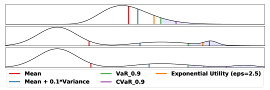
Figure 1: Comparison of different risk measures across three different distributions of costs.

A promising sampling-based approach that directly optimizes the policy for solving general nonlinear optimization problems is stochastic search. Stochastic search is a general class of optimization methods that optimizes the objective function by randomly sampling and updating candidate solutions. Many well-known algorithms, such as Cross Entropy Method (CEM) [21], genetic algorithm [22], and simulated annealing [23] fall into this category. Recently, a Gradient-based Adaptive Stochastic Search (GASS) algorithm was proposed by [24]. GASS updates the candidate solution by taking the gradient with respect to the sampling distribution parameters of solutions and approximating the gradient with Monte Carlo sampling. [25] extended GASS to constrained dynamic optimization problems, and [26] showed that Information Theoretic Model Predictive Path Integral (MPPI) [27] emerges as a special case of dynamic GASS in the case of Gaussian and Poisson sampling distributions.

In this paper, we extend the risk sensitive formulation of GASS [28] and present Risk Sensitive Stochastic Search (RS3), a general framework for solving CVaR optimization for dynamical systems. The resulting algorithm bypasses the problem of time-inconsistency by directly performing stochastic gradient descent on the sampling distribution parameters. The framework is capable of handling uncertain initial states, parameters, and system stochasticity. We demonstrate the applicability of our framework to robotics by combining it with a particle filter to perform risk-sensitive belief space control on a pendulum, cartpole and quadcopter in simulation. In addition, we show that our framework outperforms in terms of final cost in average and under other risk measures compared to a risk-sensitive distributional RL algorithm, the Sample-based Distributional Policy Gradients (SDPG) [29] on a pendulum and cartpole system in simulation.

The rest of this paper is organized as follows: in Section 2 we formulate the problem and derive the stochastic search framework. We present the algorithm and its application to belief space optimization in Section 3. The simulation results are included in Section 4. Finally, we conclude the paper in Section 5.

2 Stochastic Search

2.1 Notation, Mathematical Preliminaries, and Problem Formulation

Note that hereon we use $\mathbb{E}_{p(x)}[f(x)]$ to denote the integral $\int_{\Omega_{x}}f(x)p(x)\mathrm{d}x$ and $p(x)$ is dropped from the expectation for simplicity when it is clear which distribution the expectation is taken with respect to. We consider the problem of minimizing the CVaR of cost function $J:\mathbb{R}^{{n_{x}}\times T}\times{\cal{U}}\to\mathbb{R}^{+}$

$$U^{*}=\operatornamewithlimits{argmin}_{U\in{\cal{U}}}\text{CVaR}^{\gamma}[J(X,U)],$$ (1)

subject to nonlinear stochastic dynamics

$$x_{t+1}\sim p(x_{t+1}|x_{t},u_{t};\phi).$$ (2)

Here we have $U=\{u_{0},\cdots,u_{T-1}\}\in{\cal{U}}$ as the control path and $X=\{x_{0},\cdots,x_{T}\}\in\mathbb{R}^{n_{x}\times T}$ as the state path where $T\in[0,\infty)$ is the optimization horizon. ${\cal{U}}\subset\mathbb{R}^{n_{u}\times T-1}$ is the set of admissible control sequences, and $\phi$ is the system parameters. This formulation is capable of handling stochasticity in dynamics, $p(x_{t+1}|x_{t},u_{t})$, uncertain parameters, $p(\phi)$, and uncertain initial condition, $p(x_{0})$. The CVaR is computed with respect to the uncertainty distributions. Assuming that $p(x_{t+1}|x_{t},u_{t};\phi)$, $p(x_{0})$ and $p(\phi)$ are independent continuous density functions and $J$ is continuous, the minimization problem (1) can be rewritten as

$$U^{*}=\operatornamewithlimits{argmin}_{U\in{\cal{U}}}\mathbb{E}_{p(\chi)}[J(X,U)|J\geq\text{VaR}^{\gamma}(J)].$$ (3)

where $p(\chi)=p(x_{0})p(\phi)\prod_{t=0}^{T}p(x_{t+1}|x_{t},u_{t})$ is the joint pdf of all uncertainty distributions. We parameterize the control $u$ with a policy $\pi_{\eta}$ characterized by its parameters $\eta$. The policy can be of any functional form, i.e. open-loop ($u_{t}=v_{t},\eta_{t}=v_{t}$), linear feedback ($u_{t}=k_{t}x_{t}+v_{t},\eta_{t}=\{k_{t},v_{t}\}$) or a neural network. We then define a sampling distribution for the policy parameters from the exponential family with a pdf of the form

$$p(\eta_{t};\theta_{t})=h(\eta_{t})\exp\Big{(}\theta_{t}^{\mathrm{T}}T(\eta_{t})-A(\theta_{t})\Big{)},$$ (4)

where $\theta$ is the natural parameters of the distribution and $T(\eta)$ is the sufficient statistics of $\eta$. The minimization is now performed with respect to the natural parameters

$$\theta^{*}=\operatornamewithlimits{argmin}_{\theta\in\Theta}\mathbb{E}_{p(\chi,\theta)}[J(X,U)|J\geq\text{VaR}^{\gamma}(J)].$$ (5)

The expectation is now taken with respect to the joint distribution of uncertainty and the sampling distribution. It is easy to show that the expected cost in (5) is an upper bound on the optimal cost in (3).

2.2 Update Law Derivation

In this section we derive the gradient descent update rule for the optimization problem defined in (5). To be consistent with GASS, we turn the minimization problem into a maximization one by optimizing with respect to $-J$. We then introduce a shape function $S:\mathbb{R}\rightarrow\mathbb{R}^{+}$ which allows for different weighing schemes of the cost levels, leading to different optimization behaviors [30]. The problem is then transformed into

$$\begin{split}\theta^{*}&=\operatornamewithlimits{argmax}_{\theta\in\Theta}\mathbb{E}_{p(\theta)}[S(-\mathbb{E}_{p(\chi)}[J(X,U)|J\geq\text{VaR}^{\gamma}(J)])]\\ &=\operatornamewithlimits{argmax}_{\theta\in\Theta}\mathbb{E}_{p(\theta)}[S(-\text{CVaR}^{\gamma}[J(X,U)])].\end{split}$$ (6)

The shape function needs to satisfy the following conditions:

1. $S(y)$ is nondecreasing in $y$ and bounded from above and below for bounded $y$, with the lower bound being away from zero.

2. The set of optimal solutions $\{\operatornamewithlimits{argmax}_{y\in\mathcal{Y}}S(H(y))\}$ after the transform is a non-empty subset of the solutions $\{\operatornamewithlimits{argmax}_{y\in\mathcal{Y}}H(y)\}$ of the original problem.

Common shape functions include: 1. the identity function, $S(y)=y$; 2. the exponential function, $S(y;\kappa)=\exp(\kappa y)$, which leads to the Information Theoretic MPPI update law [27]; 3. the sigmoid function, $S(y;\kappa,\varphi)=(y-y_{\text{lb}})\tfrac{1}{1+\exp(-\kappa(y-\varphi))}$, where $y_{\text{lb}}$ is a lower bound for the cost and $\varphi$ is the ($1-\rho$)-quantile, which results in an updste law similar to CEM but with soft elite threshold $\rho$.

Finally, we apply another log transformation to obtain scale-free gradient and the optimization problem becomes

$$\theta^{*}=\operatornamewithlimits{argmax}_{\theta\in\Theta}\ln\mathbb{E}[S(-\text{CVaR}^{\gamma}[J(X,U)])]=\operatornamewithlimits{argmax}_{\theta\in\Theta}l(\theta).$$ (7)

Since $\ln:\mathbb{R}^{+}\rightarrow\mathbb{R}$ is a strictly increasing function, it does not change the maximization objective. We can now take its gradient with respect to the parameters. Writing the expectation as an integral with respect to the path probability $p(X,U;\theta)$ we get

$$\mathbb{E}[S(-\text{CVaR}^{\gamma}[J(X,U)])]=\int_{\Omega_{\eta}}S\Big{(}-\int_{\Omega_{\chi}}J(X,U)p(X,U;\theta){\mathrm{d}}\chi\Big{)}{\mathrm{d}}\eta,$$ (8)

where $\Omega_{\chi}$ is defined such that $J\geq\text{VaR}^{\gamma}(J)$ if and only if $\chi\in\Omega_{\chi}$, and $\Omega_{\eta}$ is defined such that $\pi_{\eta_{t}}(x_{t})\in{\cal{U}}_{t},\forall t$. The path probability distribution can be decomposed as

$$p(X,U;\theta) =p(x_{T}|x_{T-1},\pi_{\eta}(x_{T-1});\phi)p(\eta_{T-1};\theta_{T-1})\cdots p(x_{0})p(\phi)$$ (9)

$$=\underbrace{p(x_{0})p(\phi)\prod_{t=0}^{T-1}p(x_{t+1}|x_{t},\pi_{\eta}(x_{t});\phi)}_{p(\chi)}\underbrace{\prod_{t=0}^{T-1}p(\eta_{t};\theta_{t})}_{p(\eta)}.$$ (10)

Note that since the uncertainty and sampling distribution are independent, their joint distribution can be broken into the product of the two. The gradient of the objective function (7) with respect to the parameters can be taken as

$$\nabla_{\theta}l(\theta)=\frac{\mathbb{E}[S(-\text{CVaR}^{\gamma}[J(X,U)])\nabla_{\theta}\big{(}\sum_{t=0}^{T-1}\ln p(\eta_{t};\theta_{t})\big{)}]}{\mathbb{E}[S(-\text{CVaR}^{\gamma}[J(X,U)])]}.$$ (11)

Appendix B . The gradient of the log parameter distribution at each time step can be calculated as

$$\nabla_{\theta_{t}}\ln p(\eta_{t};\theta_{t}) =\nabla_{\theta_{t}}\ln\Big{(}h(\eta_{t})\exp\Big{(}\theta_{t}^{\mathrm{T}}T(\eta_{t})-A(\theta_{t})\Big{)}\Big{)}$$ (12)

$$=\nabla_{\theta_{t}}(\theta_{t}^{\mathrm{T}}T(\eta_{t})-A(\theta_{t}))$$ (13)

$$=T(\eta_{t})-\nabla_{\theta_{t}}A(\theta_{t}).$$ (14)

Plugging it back into the gradient of the cost function, we get

$$\nabla_{\theta_{t}}l(\theta)=\frac{\mathbb{E}[S(-\text{CVaR}^{\gamma}[J(X,U)])(T(\eta_{t})-\nabla_{\theta_{t}}A(\theta_{t}))]}{\mathbb{E}[S(-\text{CVaR}^{\gamma}[J(X,U)])]}.$$ (15)

With this, we have a gradient ascent update law for the parameters as

$$\theta_{t}^{k+1}=\theta_{t}^{k}+\alpha^{k}\nabla_{\theta_{t}}l(\theta^{k}).$$ (16)

where the step size sequence $\alpha^{k}$ satisfies the typical assumptions in Stochastic Approximation (SA):

$$\alpha^{k}>0\quad\forall k,\quad\lim_{k\to\infty}\alpha^{k}=0,\quad\sum_{k=0}^{\infty}\alpha_{k}=\infty$$ (17)

2.3 Practical Considerations

Numerical Approximation: The CVaR of the cost can be approximated [31] with

$$\hat{C}_{n}^{\gamma} =\hat{V}_{n}^{\gamma}+\frac{1}{M(1-\gamma)}\sum_{m=1}^{M}J_{n,m}-\hat{V}_{n}^{\gamma}\big{)}^{+}$$ (18)

$$\hat{V}_{n}^{\gamma} =\inf\{x:\frac{1}{M}\sum_{m=1}^{M}\mathbbm{1}_{\{J_{n,m}\leq x\}}\geq\gamma\}.$$ (19)

The outer expectation can be approximated as $\mathbb{E}[S(-\text{CVaR}^{\gamma}[J(X,U)])]=\frac{1}{N}\sum_{n=1}^{N}S(-\hat{C}^{\gamma}_{n})$. Note that the expectation and CVaR in (15) are computed as averages over costs defined on entire trajectory samples.

Model Predictive Control Formulation: The parameter update in Equation 16 can be used for trajectory optimization as well as in a receding horizon or Model Predictive Control (MPC) fashion. MPC is a powerful algorithmic approach to nonlinear feedback control which is essential in tasks that involve risk measures or high order statistical characteristics of cost functions. In this paper we will leverage parallelization using GPUs to implement Equation 16 in MPC fashion.

Adaptive Stochastic Search: The MPC formulation allows online interaction with the stochastic system dynamics. Data from this online interaction can be used to feed adaptive or state estimation schemes that update the probability distribution $p(\chi)$ in an online fashion. In this work, we make use of a nonlinear state estimator, namely a particle filter, to propagate and update distribution $p(\chi)$ over time. The resulting control architecture is a sampling-based risk-sensitive adaptive MPC scheme that optimizes CVaR while adapting the probability distribution over parametric uncertainties. The details of this approach are further explained in the next section.

3 Algorithm

In this section we present the RS3 algorithm implemented in MPC fashion, as shown in Algorithm 1. At initial time, the policy parameter distribution’s natural parameters are initialized. Given an initial state and parameter distribution provided by an estimator, $M$ i.i.d. samples are obtained. $N$ policies are sampled from the policy parameter distribution and each copy of the policy is applied to all $M$ samples of the initial states. In the case of stochastic dynamics, the states of each of the $M$ samples are propagated with an independent realization of the stochastic dynamics. A cost is then calculated for each of the total $N\times M$ trajectories. For each policy sample, its associated CVaR cost is approximated with the $M$ cost samples using (18) and (19). Using the CVaR values, the policy parameter distributions’ natural parameters can be updated using (15) and (16). In our simulations, we use Gaussian distributions with fixed variance to sample policy parameters, for which the sufficient statistics are $T(\eta_{t})=\eta_{t}$ and $\nabla_{\theta_{t}}A(\theta_{t})=\mathbb{E}[T(\eta_{t})]$. The parameter update step is detailed in algorithm 2. As is common in SA algorithms, Polyak averaging is performed on the natural parameters to improve the convergence rate [32]. With the Polyak averaged natural parameters $\bar{\eta}$, an optimal policy can be sampled and applied to the system for $\tau$ timesteps. Finally, we apply a shift operator $\omega(\theta,\tau)$ that recedes the optimization horizon and outputs $\tilde{\theta}_{t}=\theta_{t+\tau}$. The last $\tau$ timesteps of the natural parameters are re-initialized.

Note that the RS3 algorithm can handle any or all uncertainties from initial state distribution, uncertain parameters and stochastic dynamics provided that i.i.d. samples can be generated from the uncertain distribution.

In our simulation examples of belief space control, we use a particle filter to provide the initial state distribution. To handle uncertain model parameters, we augment the states by the uncertain parameters and use a particle filter to learn its distribution (detailed in Appendix C) . In both cases, i.i.d. particles from non-Gaussian distributions can be used directly used in the RS3 algorithm. However, we want to stress that any filter can be used together with the RS3 algorithm.

4 Simulation Results

In this section, we showcase the general applicability of RS3 in dealing various types of uncertainty. 1) External noise: Comparing its performance against the SDPG algorithm for CVaR optimization. 2) Uncertain system parameters: combining it with a particle filter to perform risk sensitive control in belief space. 3) Uncertain initial condition: This can be found in Section D.1.

All simulations were performed with a risk level of $0.9$. The open loop policy $\pi_{\eta}(x)=\eta$ is used for all simulations, where $\eta$ directly maps to the controls. The multivariate normal distribution is chosen as the sampling distribution, and we use the method proposed in [25] to handle the box control constraints in the simulation tasks by sampling from a truncated multivariate normal distribution. The tuning parameters of all simulations are included in the Appendix.

4.1 Comparison Against Sample-based Distributional Policy Gradients

The Sample-based Distributional Policy Gradients algorithm [33, 29] is one of the most recent work on optimizing CVaR for dynamical systems. SDPG [33] and the risk-sensitive version of SDPG [29] are actor-critic type policy gradient algorithms in the distributional RL [34] setting.

The actor network parameterizes the policy and the critic network learns the return distribution by reparameterizing simple Gaussian noise samples. The risk-sensitive version of SDPG [29] is an extension of the naive SDPG [33] algorithm by using CVaR as a loss function to train the actor network to learn a risk-sensitive policy. We compared RS3 and the risk-sensitive SDPG on two classic control systems in OpenAI Gym [35], a pendulum and a cartpole.

Table 1: Reward comparison results between RS3 (ours) vs. risk-sensitive SDPG [29]

System		Pendulum				Cartpole
Noise variance		0.3	1.0	2.0	3.0	0.3	1.0	2.0
	Mean	169.2	172.0	177.0	183.1	291.0	299.3	311.9
RS3	VaR	170.3	175.9	185.1	196.1	291.9	302.5	320.1
	CVaR	170.7	177.6	189.3	203.7	292.3	304.2	326.9
	Mean	171.1	173.4	178.4	185.2	302.1	430.4	591.3
SDPG	VaR	172.4	177.9	188.3	201.1	302.6	607.9	650.8
	CVaR	172.9	179.5	191.6	206.8	302.8	617.8	659.6

Figure 2: The histograms of the final cost in the case of injected control noise sampled from $\mathcal{N}(0,1).$ Left: Pendulum, Right: Cartpole.

Typical RL algorithms always receive some state feedback either fully or partially from environments. Thus, to fairly compare against SDPG, we exploited an MPC scheme in RS3 to implicitly receive the state feedback and perform a receding-horizon optimization. In addition, as SDPG is unable to handle uncertainty in the initial states and controls, we consider deterministic initial states and system dynamics with additive noise h the control channels. To match the RS3 framework, the Gym environment’s controls were modified to be continuous and use a quadratic cost function instead of the typical RL reward function -1, 0, or +1 implemented in Gym. The cost function used in the simulation can be found in Appendix D.1.1. All other training parameters for risk-sensitive SDPG were the same as the parameters used in the original work [29].

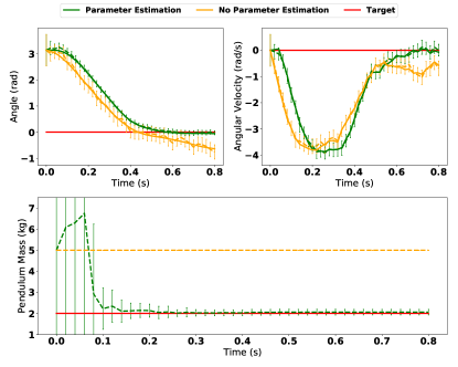
Figure 3: Nonlinear belief space optimization with uncertain pendulum mass in the Pendulum problem.

Under the aforementioned conditions, RS3 is shown to outperform SDPG overall by converging to a lower CVaR value, especially in the case of larger noise levels. The mean, VaR, and CVaR values of the final costs obtained from both algorithms for the pendulum and cartpole simulation are shown in Table 1 and a comparison of the histogram of the final costs are shown in Figure 2. The state, control, and cost histograms for all the simulation in Table 1 can be found in Section D.1.

It is clearly shown in Figure 2 that the distribution of the final cost has sharper tail on the high cost region in RS3’s results compared to SDPG’s. As a result, the mean, VaR, and CVaR of RS3’s final costs are smaller than SDPG’s.

The reason why our method outperforms the RL framework is that we perform online update of our policy whereas the RL policy is fixed after training. This disadvantage of RL algorithms comes from the nature of RL. Once a model is trained on a specific dataset or with a specific noise profile, the model fails to output correct predictions under a new environment or given unseen inputs or noise. Our online optimization scheme solves this issue and fits better in risk-sensitive control.

4.2 Belief Space Optimization

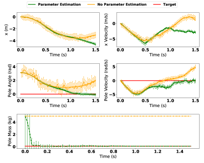
Figure 4: Nonlinear belief space optimization with uncertain pole mass in the Cartpole problem.

We next show results for the uncertain parameter case from the pendulum, cartpole and quadcopter systems. In each trajectory plot, the dotted lines represent estimates from the particle filter with the error bars showing the $\pm 3\sigma$ uncertainties of the nonlinear belief. The solid line represents the ground truth states.

Pendulum: We first apply RS3 to a pendulum for a swingup task with unknown pendulum mass. We assume deterministic initial condition and state transition model. The pendulum’s true mass is set to $2$ kg. The prior for pendulum mass is set to be ${\cal N}(5.0,4.0)$. The initial states $\mathbf{x}=[\theta,\dot{\theta}]$ are drawn from a normal distribution with mean $[\pi,0]$ and covariance matrix $\textrm{diag}([0.1,0.1])$. We assume full-state observability with additive measurement noise $\xi\sim\mathcal{N}(0,1)$. From Figure 3, we can observe that RS3 is able to correctly estimate the mass of the pendulum in the parameter estimation case. Without parameter estimation, RS3 overestimates the control effort required and overshoots the target angle.

Cartpole: We apply the proposed algorithm to the task of cartpole swingup with with unknown pole mass. The prior over the mass of the pole is a normal distribution $\mathcal{N}(5.0,5.0)$ and the true value is $0.1\text{\,}\mathrm{k}\mathrm{g}$. Our algorithm is able to learn the true mass of the pole and successfully perform a swing up (Figure 4). We compare this with the case of not estimating the mass of the pole, where the algorithm does not sample from the correct dynamics and is unable to correctly optimize for a trajectory that successfully swings up.

Quadcopter: Finally, we apply our algorithm to the quadcopter system (dynamics can be found in [36]), where the task is to fly a quadcopter with states $[x,y,z,\dot{x},\dot{y},\dot{z},r,p,y,\dot{r},\dot{p},\dot{y}]$ from $[0,0,0]$ to $[2,2,2]$. The drag coefficient of the system is unknown, the prior over the drag is a normal distribution $\mathcal{N}(0.5,0.5)$ and the true value is $0.1$. The algorithm is once again able to learn the correct drag coefficient and manages to pilot the quadcopter to the target position without significant overshoot despite the drag coefficient being $500\%$ larger than the mean of the prior (Figure 5). For the case where we do not perform parameter estimation, since the prior of the drag coefficient is greater than the actual value, the control policy found by the RS3 framework results in overshooting behavior before convergence, although it still manages to converge to the target state due to the robustness from optimizing for CVaR.

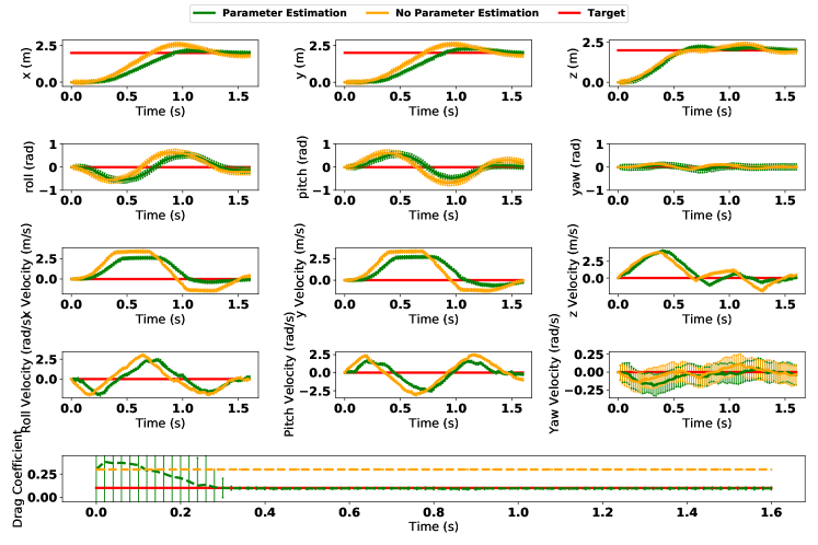
Figure 5: Nonlinear belief space optimization with uncertain drag coefficient in the Quadcopter problem. RS3 with parameter estimation is able to converge much closer in roll, pitch and pitch velocity compared to without parameter estimation.

5 Conclusion

In this paper we introduced a general framework for CVaR optimization for dynamical systems. The resulting algorithm, RS3, is capable of handling uncertainties arising from uncertain initial conditions, unknown model parameters and system stochasticity. The algorithm can be readily combined with any filter for belief space risk sensitive control. We compared RS3 against SDPG on the systems of a pendulum and cartpole and demonstrated outperformance in terms of final CVaR cost. In addition, we combined RS3 with a particle filter for adaptive risk-sensitive control on non-Gaussian belief under different sources of uncertainty.

Appendix A Coherent Risk Measures

A risk measure $\rho:\mathcal{L}\rightarrow\mathbb{R}\cup\{+\infty\}$ is coherent if it satisfies certain simple mathematical properties including:

1. Monotonicity: If $X_{1},X_{2}\in\mathcal{L}$ and $X_{1}\leq X_{2}$ a.s., then $\rho(X_{1})\leq\rho(X_{2})$.

2. Sub-additivity: If $X_{1},X_{2}\in\mathcal{L}$, then $\rho(X_{1}+X_{2})\leq\rho(X_{1})+\rho(X_{2})$.

3. Positive homogeneity: If $\alpha\geq 0$ and $X\in\mathcal{L}$, then $\rho(\alpha X)=\alpha\rho(X)$.

4. Translation invariance: If $X\in\mathcal{L}$ and $c\in\mathbb{R}$ is constant, then $\rho(X+c)=\rho(X)+c$.

Note that VaR does not respect the sub-additivity property.

Appendix B Stochastic Search Update Law Derivation

The stochastic search update law (11) can be derived as

$$\nabla_{\theta_{t}}l(\theta) =\frac{\nabla_{\theta}\mathbb{E}[S(-\text{CVaR}^{\gamma}[J(X,U)])]}{\mathbb{E}[S(-\text{CVaR}^{\gamma}[J(X,U)])]}$$

$$=\frac{\nabla_{\theta}\int_{\Omega_{\eta}}S(-\text{CVaR}^{\gamma}[J(X,U)])p(\eta){\mathrm{d}}\eta}{\mathbb{E}[S(-\text{CVaR}^{\gamma}[J(X,U)])]}$$

$$=\frac{\int_{\Omega_{\eta}}S(-\text{CVaR}^{\gamma}[J(X,U)])\nabla_{\theta}p(\eta){\mathrm{d}}\eta}{\mathbb{E}[S(-\text{CVaR}^{\gamma}[J(X,U)])]}$$

$$=\frac{\int_{\Omega_{\eta}}S(-\text{CVaR}^{\gamma}[J(X,U)])p(\eta)\nabla_{\theta}\ln p(\eta){\mathrm{d}}\eta}{\mathbb{E}[S(-\text{CVaR}^{\gamma}[J(X,U)])]}$$

$$=\frac{\int_{\Omega_{\eta}}S(-\text{CVaR}^{\gamma}[J(X,U)])p(\eta)\nabla_{\theta}\big{(}\sum_{t=0}^{T-1}p(\eta_{t};\theta_{t})\big{)}{\mathrm{d}}\eta}{\mathbb{E}[S(-\text{CVaR}^{\gamma}[J(X,U)])]}$$

$$=\frac{\mathbb{E}[S(-\text{CVaR}^{\gamma}[J(X,U)])\nabla_{\theta}\big{(}\sum_{t=0}^{T-1}\ln p(\eta_{t};\theta_{t})\big{)}]}{\mathbb{E}[S(-\text{CVaR}^{\gamma}[J(X,U)])]}.$$

Appendix C Particle Filter and RS3 for Uncertain Model Parameters

In the case of unknown parameters $\phi$ in the model, we use the particle filter to learn both the states and uncertain model distribution. We first augment our state space with those parameters as $y=[x,\phi]^{\mathsf{T}}$ and formulate the new dynamics as

$$y_{t+1} =\begin{bmatrix}f(x_{t},u_{t},\phi_{t})\\ 1\end{bmatrix}+\begin{bmatrix}0\\ w_{t}\end{bmatrix},\quad\phi_{0}\sim p(\phi_{0})$$

$$z_{t} =h(x_{t})+v_{t}$$

where $w_{t}$ is the process noise added to mitigate the sample impoverishment problem of the particle filter. Starting with deterministic initial states $x_{0}$ and a prior distribution on the parameters $p(\phi_{0})$. The steps of this adaptive risk sensitive control framework at each timestep are

1. Sample from initial distribution: $\{\hat{y}_{t}^{i}\}_{i=1,\dots,M}\sim p(y_{t})$

2. Compute policy: $\eta_{t}=\text{RS3}(\{\hat{y}_{t}^{i}\}_{i=1,\dots,M})$

3. Apply control: $x_{t+1}\leftarrow F(x_{t},\pi_{\eta_{t}}(x_{t}),0;\phi)$

4. Obtain observation: $z_{t+1}\leftarrow h(x_{t+1},\xi_{t+1})$

5. Propagate particles: $\{\hat{x}_{t+1}^{i}\}_{i=1,\dots,M}\leftarrow\hat{F}(u_{t},\{\hat{x}_{t}^{i}\}_{i=1,\dots,M},0;\{\hat{\phi}_{t}^{i}\}_{i=1,\dots,M})$

6. Update likelihood: $\{q_{i}\}_{i=1,\dots,M}=L(z_{t+1},\{\hat{x}_{t+1}^{i}\}_{i=1,\dots,M})$

where $F$ is the true system dynamics with real parameters $\phi$ and $\hat{F}$ is the model for particle filter and RS3, and both do not contain stochasticities in the dynamics. $\xi$ is the observation noise.

Appendix D Additional Simulation Results

D.1 Comparison against SDPG

D.1.1 Cost function

We define the cost function $J(X,U)$ as

$$J(X,U) =g(x_{T})+\sum_{t=t_{0}}^{T-1}l(x_{t},u_{t}),$$ (20)

where $x_{t}\in\mathbb{R}^{n_{x}}$ is the state at time $t$, $u_{t}\in\mathbb{R}^{n_{u}}$ is the control at time $t$, $g$ is the state cost at the final time $T$, and $l$ is the running cost at time $t$. In the simulations, we set $g=l$ and the running cost is composed of the quadratic state cost $(x_{t}-x_{target})^{\mathsf{T}}Q(x_{t}-x_{target})$ and the quadratic control cost $u_{t}^{\mathsf{T}}Ru_{t}$.

The system dynamics are from OpenAI Gym [35] and the pendulum state is defined as $[\theta,\dot{\theta}]$, the pendulum angle and the angular velocity. The cartpole state is defined as $[x,\dot{x},\theta,\dot{\theta}]$, the cart position, position velocity, pole angle, and the pole angular velocity. The state and control cost used in pendulum dynamics are $Q=\text{diag}([3,0.01])$, where $\text{diag}()$ represents a diagonal matrix, and $R=0.01$. In cartpole, the costs are $Q=\text{diag}([0.01,0.1,1,0.1])$ and $R=0.001$.

For Pendulum, the initial state is $[-\pi,0]$ and target state is $[0,0]$ and for the Cartpole, the initial state is $[0,0,-\pi,0]$ and target state is $[0,0,0,0]$.

D.1.2 Pendulum

Four different levels of control noise are tested in the pendulum simulations comparing RS3 against SDPG: $\mathcal{N}(0,0.3^{2}),\mathcal{N}(0,1.0^{2}),\mathcal{N}(0,2.0^{2}),$ and $\mathcal{N}(0,3.0^{2})$. The mass of the pendulum is set to $1\text{\,}\mathrm{kg}$ and its length is set to $1.0\text{\,}\mathrm{m}$. The controls are constrained by the box constraints $\left\lvert u_{t}\right\rvert<10$. The results can be found in the figures below. As discussed in the main paper and can be observed from Figure 6 to Figure 9, RS3 outperforms SDPG in terms of the Mean, VaR, and CVaR of the final costs in all cases.

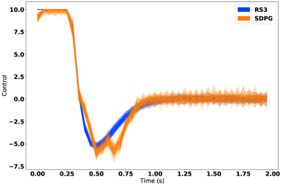
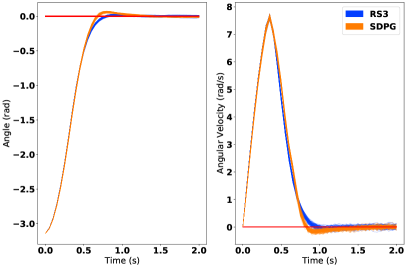
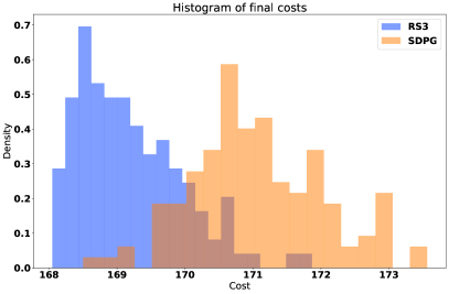
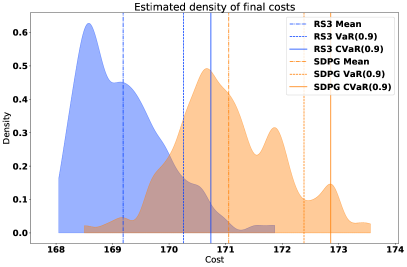
Figure 6: Top: Control and state trajectories from the Pendulum problem with noise in the control channel. The control noise is $\mathcal{N}(0,0.3^{2}).$ Bottom: Cost histogram and the estimated p.d.f. of it.

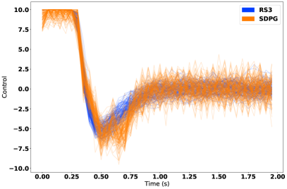
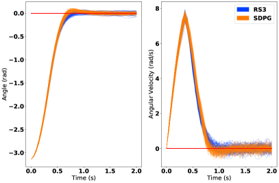
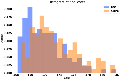
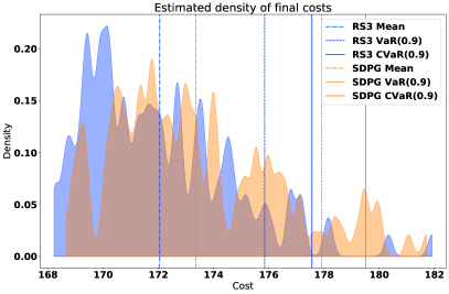
Figure 7: Top: Control and state trajectories from the Pendulum problem with noise in the control channel. The control noise is $\mathcal{N}(0,1.0^{2}).$ Bottom: Cost histogram and the estimated p.d.f. of it.

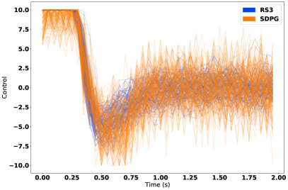
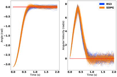
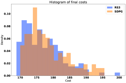
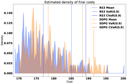
Figure 8: Top: Control and state trajectories from the Pendulum problem with noise in the control channel. The control noise is $\mathcal{N}(0,2.0^{2}).$ Bottom: Cost histogram and the estimated p.d.f. of it.

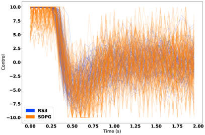
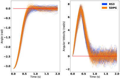
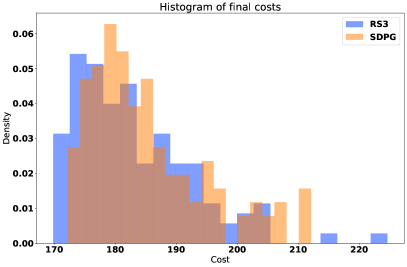
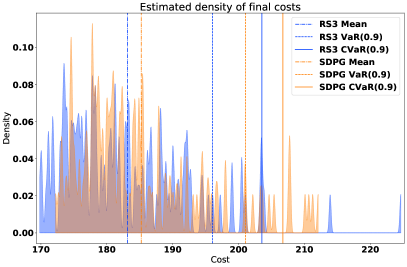
Figure 9: Top: Control and state trajectories from the Pendulum problem with noise in the control channel. The control noise is $\mathcal{N}(0,3.0^{2}).$ Bottom: Cost histogram and the estimated p.d.f. of it.

D.1.3 Cartpole

Similarly, 3 different levels of additive control noise were used to compare RS3 and SDPG in the cartpole problem: $\mathcal{N}(0,0.3^{2}),\mathcal{N}(0,1.0^{2}),$ and $\mathcal{N}(0,2.0^{2})$. The mass of the cart are set to $1\text{\,}\mathrm{kg}$, the mass of the pole $0.1\text{\,}\mathrm{kg}$ and its length $0.5\text{\,}\mathrm{m}$. The controls are constrained by the box constraints $\left\lvert u_{t}\right\rvert<15$. The results can be found in Figure 10 to Figure 12.

Although the control becomes spiky with larger noise, RS3 is able to accomplish the task, whereas SDPG fails the task most of the time, as seen in Figure 11 and Figure 12. These results show that RS3 does a better job of risk-sensitive control on higher order systems compared to SDPG.

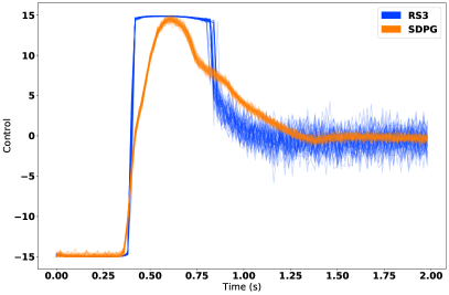
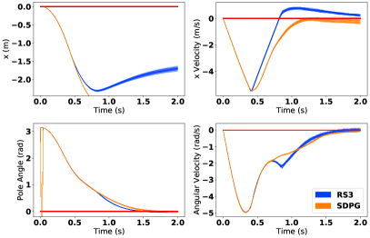
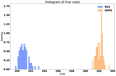
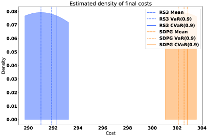
Figure 10: Top: Control and state trajectories from the Cartpole problem with noise in the control channel. The control noise is $\mathcal{N}(0,0.3^{2}).$ Bottom: Cost histogram and the estimated p.d.f. of it.

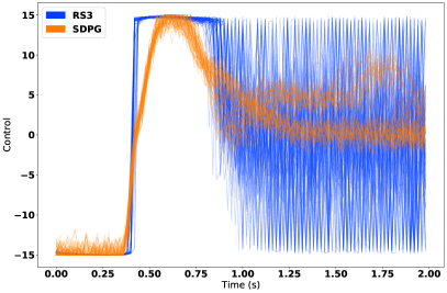
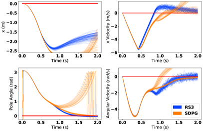
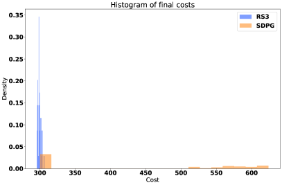
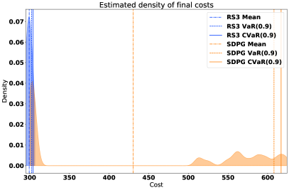
Figure 11: Top: Control and state trajectories from the Cartpole problem with noise in the control channel. The control noise is $\mathcal{N}(0,1.0^{2}).$ Bottom: Cost histogram and the estimated p.d.f. of it.

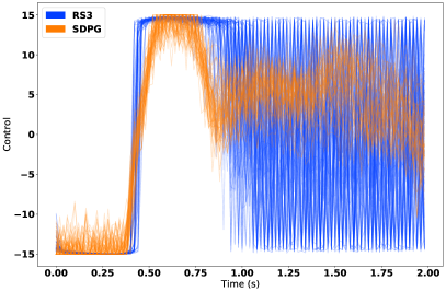
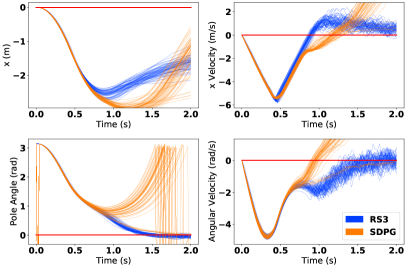
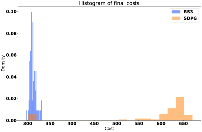
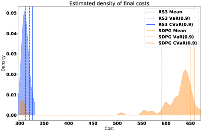
Figure 12: Top: Control and state trajectories from the Cartpole problem with noise in the control channel. The control noise is $\mathcal{N}(0,2.0^{2}).$ Bottom: Cost histogram and the estimated p.d.f. of it.

Appendix E Belief Space Risk Sensitive Control

E.1 Pendulum

We test RS3 on Pendulum in the case of uncertainty in the initial conditions and in the case of stochastic dynamics where the true state of the system is fully observable. The mass of the pendulum is set to $1\text{\,}\mathrm{kg}$ and its length is set to $1.0\text{\,}\mathrm{m}$. The controls are constrained by the box constraints $\left\lvert u_{t}\right\rvert<10$. Measurements of the state $x$ are corrupted with additive noise $\xi\sim\mathcal{N}(0,\textrm{diag}([0.7,0.3]))$. In the case of uncertain initial states, the initial states $x_{0}=[\theta,\dot{\theta}]$ are drawn from a normal distribution with mean $[\pi,0]$ and covariance matrix $\textrm{diag}([0.5,0.5])$. In the case of stochastic dynamics, the controls are corrupted by noise with distribution $\mathcal{N}(0,3.0^{2})$.

The results for uncertain initial conditions and stochastic dynamics can be found in Figure 13 and Figure 14 respectively.

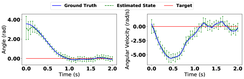
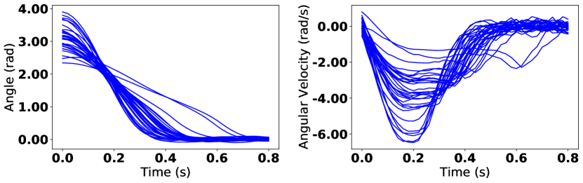
Figure 13: Trajectories from the Pendulum problem with is uncertainty in the initial conditions. Top: A comparison of the posterior state from the particle filter and the ground truth from a single trajectory. Bottom: Different trajectory realizations of the initial condition.

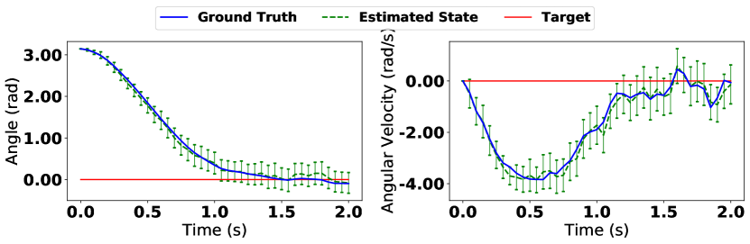
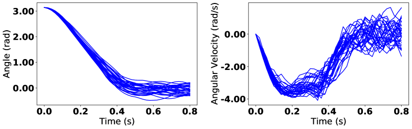
Figure 14: Trajectories from the Pendulum problem with stochastic dynamics. Top: A comparison of the posterior state from the particle filter and the ground truth from a single trajectory. Bottom: Different trajectory realizations of the stochastic dynamics.

E.2 Cartpole

Similarly, we test RS3 on Cartpole in the case of uncertainty in the initial conditions and in the case of stochastic dynamics. The mass of the cart are set to $1\text{\,}\mathrm{kg}$, the mass of the pole $0.1\text{\,}\mathrm{kg}$ and its length $0.5\text{\,}\mathrm{m}$. The controls are constrained by the box constraints $\left\lvert u_{t}\right\rvert<15$. Measurements of the state $x$ are corrupted with additive noise $\xi\sim\mathcal{N}(0,\textrm{diag}([1,1,0.25,0.25]))$.

The initial states $x_{0}=[x,\dot{x},\theta,\dot{\theta}]$ are drawn from a normal distribution with mean $[0,0,\pi,0]$ and covariance matrix $\textrm{diag}([0.5,0.5,0.08,0.05])$

The results for uncertain initial conditions and stochastic dynamics can be found in Figure 15 and Figure 16 respectively.

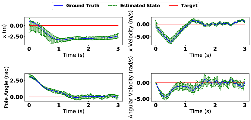
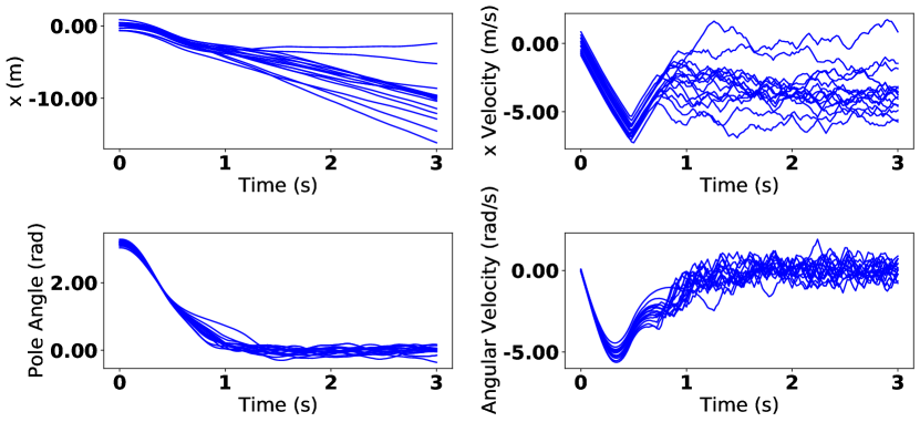
Figure 15: Trajectories from the Cartpole problem with is uncertainty in the initial conditions. Top: A comparison of the posterior state from the particle filter and the ground truth from a single trajectory. Bottom: Different trajectory realizations of the initial condition.

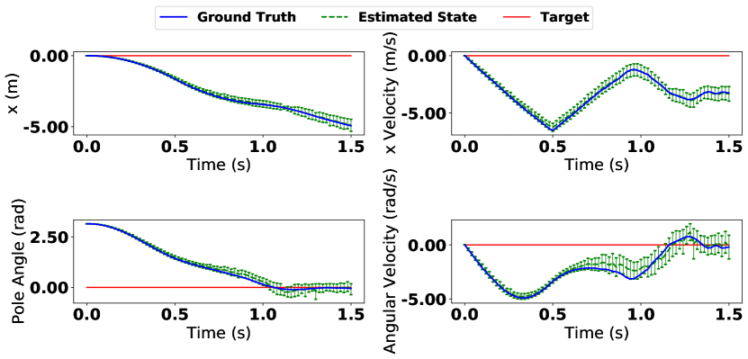
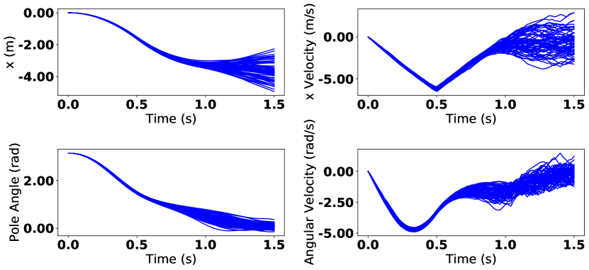
Figure 16: Trajectories from the Cartpole problem with stochastic dynamics. Top: A comparison of the posterior state from the particle filter and the ground truth from a single trajectory. Bottom: Different trajectory realizations of the stochastic dynamics.

E.3 Quadcopter

Finally, we test RS3 on the Quadcopter in the case of uncertainty in the initial conditions and stochastic dynamics. Measurements of the state $x$ are corrupted with additive noise $\xi\sim\mathcal{N}(0,\textrm{diag}([0.1,0.1,0.1,0.01,0.01,0.01,0.08,0.08,0.08,0.01,0.1,0.01]))$. The controls are constrained by the box constraints $[0,-10,-10,-1]<u_{t}<[20,10,10,1]$.

For the case of uncertain initial states, the states $x_{0}=[x,y,z,\alpha,\beta,\gamma,\dot{x},\dot{y},\dot{z},\dot{\alpha},\dot{\beta},\dot{\gamma}]$ are drawn from a normal distribution with zero mean and covariance matrix $\textrm{diag}([0.3,0.3,0.3,0.2,0.2,0.2,0.2,0.2,0.2,0.2,0.2,0.2])$. In the case of stochastic dynamics, the controls are corrupted with noise drawn from $\mathcal{N}(0,\textrm{diag}([1,1,1,0.1])$

The results can be found in Figure 17 and Figure 18 respectively.

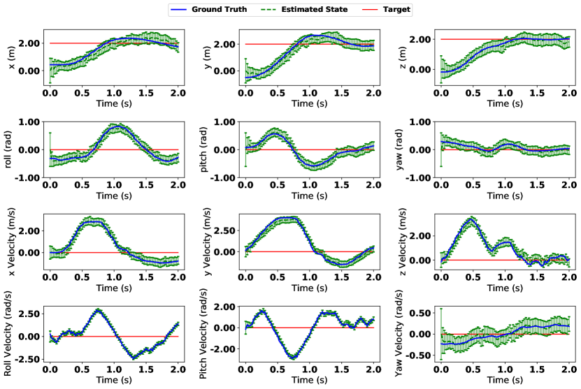
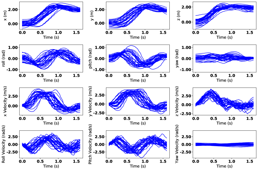
Figure 17: Trajectories from the Quadcopter problem with is uncertainty in the initial conditions. Top: A comparison of the posterior state from the particle filter and the ground truth from a single trajectory. Bottom: Different trajectory realizations of the initial condition.

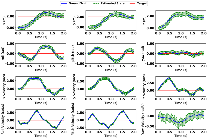
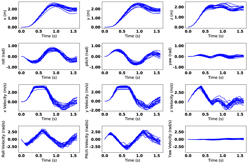
Figure 18: Trajectories from the Quadcopter problem with stochastic dynamics. Top: A comparison of the posterior state from the particle filter and the ground truth from a single trajectory. Bottom: Different trajectory realizations of the stochastic dynamics.

E.4 Parameters

To alleviate the particle degeneracy problem from particle filters, artificial process noise is added to each sample. The artificial process noises added are zero mean, and their covariances are

$$\Sigma_{\textrm{Pendulum\_est}} =\textrm{diag}([$1\text{\times}{10}^{-5}$,$1\text{\times}{10}^{-5}$,$1\text{\times}{10}^{-9}$])$$

$$\Sigma_{\textrm{Pendulum\_no\_est}} =\textrm{diag}([0.2,0.2,0])$$

$$\Sigma_{\textrm{Cartpole\_est}} =\textrm{diag}([0.001,0.001,0.001,0.001,$1\text{\times}{10}^{-6}$])$$

$$\Sigma_{\textrm{Cartpole\_no\_est}} =\textrm{diag}([0.1,0.3,0.3,0.2,$1\text{\times}{10}^{-6}$,0])$$

$$\Sigma_{\textrm{Quadcopter\_est}} =\textrm{diag}([0.02,0.02,0.02,0.03,0.03,0.03,0.04,0.04,0.04,0.04,0.04,0.04,0.001])$$

$$\Sigma_{\textrm{Quadcopter\_no\_est}} =\textrm{diag}([0.05,0.05,0.05,0.03,0.03,0.003,0.04,0.04,0.04,0.04,0.04,0.04,$1\text{\times}{10}^{-9}$])$$

where the est subscript denotes the case of uncertain parameters and no_est denotes the cases of uncertain initial condition and stochastic dynamics. Note that the required artificial process noise is much higher for simulation runs that do not estimate the parameters. This is because the incorrect priors for the parameters result in dynamics that are very different from ground truth, leading to the particle filter diverging very quickly.

References

- [1] Abhijit Gosavi. Variance-penalized markov decision processes: Dynamic programming and reinforcement learning techniques. International Journal of General Systems, 43(6):649–669, 2014.
- [2] Dotan Di Castro, Aviv Tamar, and Shie Mannor. Policy gradients with variance related risk criteria. arXiv preprint arXiv:1206.6404, 2012.
- [3] Ronald A Howard and James E Matheson. Risk-sensitive markov decision processes. Management science, 18(7):356–369, 1972.
- [4] Wendell H Fleming and William M McEneaney. Risk-sensitive control on an infinite time horizon. SIAM Journal on Control and Optimization, 33(6):1881–1915, 1995.
- [5] Philippe Jorion. Value at risk. 2000.
- [6] Philippe Artzner, Freddy Delbaen, Jean-Marc Eber, and David Heath. Coherent measures of risk. Mathematical finance, 9(3):203–228, 1999.
- [7] R Tyrrell Rockafellar, Stanislav Uryasev, et al. Optimization of conditional value-at-risk. Journal of risk, 2:21–42, 2000.
- [8] Vikas Agarwal and Narayan Y Naik. Risks and portfolio decisions involving hedge funds. The Review of Financial Studies, 17(1):63–98, 2004.
- [9] Pavlo Krokhmal, Jonas Palmquist, and Stanislav Uryasev. Portfolio optimization with conditional value-at-risk objective and constraints. Journal of risk, 4:43–68, 2002.
- [10] Shushang Zhu and Masao Fukushima. Worst-case conditional value-at-risk with application to robust portfolio management. Operations research, 57(5):1155–1168, 2009.
- [11] Antonio J Conejo, Miguel Carrión, Juan M Morales, et al. Decision making under uncertainty in electricity markets, volume 1. Springer, 2010.
- [12] Juan M Morales, Antonio J Conejo, and Juan Pérez-Ruiz. Short-term trading for a wind power producer. IEEE Transactions on Power Systems, 25(1):554–564, 2010.
- [13] Xin Chen, Melvyn Sim, David Simchi-Levi, and Peng Sun. Risk aversion in inventory management. Operations Research, 55(5):828–842, 2007.
- [14] Tomas Bjork and Agatha Murgoci. A general theory of markovian time inconsistent stochastic control problems. Available at SSRN 1694759, 2010.
- [15] Alexander Shapiro, Darinka Dentcheva, and Andrzej Ruszczyński. Lectures on stochastic programming: modeling and theory. SIAM, 2014.
- [16] Yinlam Chow and Marco Pavone. A time consistent formulation of risk constrained stochastic optimal control. arXiv preprint arXiv:1503.07461, 2015.
- [17] Georg Ch Pflug and Alois Pichler. Time-inconsistent multistage stochastic programs: Martingale bounds. European Journal of Operational Research, 249(1):155–163, 2016.
- [18] Yinlam Chow, Aviv Tamar, Shie Mannor, and Marco Pavone. Risk-sensitive and robust decision-making: a cvar optimization approach. In Advances in Neural Information Processing Systems, pages 1522–1530, 2015.
- [19] Nicole Bäuerle and Jonathan Ott. Markov decision processes with average-value-at-risk criteria. Mathematical Methods of Operations Research, 74(3):361–379, 2011.
- [20] Aviv Tamar, Yonatan Glassner, and Shie Mannor. Policy gradients beyond expectations: Conditional value-at-risk. arXiv preprint arXiv:1404.3862, 2014.
- [21] Reuven Y Rubinstein and Dirk P Kroese. The cross-entropy method: a unified approach to combinatorial optimization, Monte-Carlo simulation and machine learning. Springer Science & Business Media, 2013.
- [22] G Zames, NM Ajlouni, NM Ajlouni, NM Ajlouni, JH Holland, WD Hills, and DE Goldberg. Genetic algorithms in search, optimization and machine learning. Information Technology Journal, 3(1):301–302, 1981.
- [23] Scott Kirkpatrick, C Daniel Gelatt, and Mario P Vecchi. Optimization by simulated annealing. science, 220(4598):671–680, 1983.
- [24] Enlu Zhou and Jiaqiao Hu. Gradient-based adaptive stochastic search for non-differentiable optimization. IEEE Transactions on Automatic Control, 59(7):1818–1832, 2014.
- [25] George I Boutselis, Ziyi Wang, and Evangelos A Theodorou. Constrained sampling-based trajectory optimization using stochastic approximation. arXiv preprint arXiv:1911.04621, 2019.
- [26] Ziyi Wang, Grady Williams, and Evangelos A Theodorou. Information theoretic model predictive control on jump diffusion processes. In 2019 American Control Conference (ACC), pages 1663–1670. IEEE, 2019.
- [27] Grady Williams, Nolan Wagener, Brian Goldfain, Paul Drews, James M Rehg, Byron Boots, and Evangelos A Theodorou. Information theoretic mpc for model-based reinforcement learning. In 2017 IEEE International Conference on Robotics and Automation (ICRA), pages 1714–1721. IEEE, 2017.
- [28] Helin Zhu, Joshua Hale, and Enlu Zhou. Simulation optimization of risk measures with adaptive risk levels. Journal of Global Optimization, 70(4):783–809, 2018.
- [29] Rahul Singh, Qinsheng Zhang, and Yongxin Chen. Improving robustness via risk averse distributional reinforcement learning. The 2nd Annual Conference on Learning for Dynamics and Control (L4DC), 2020.
- [30] Yann Ollivier, Ludovic Arnold, Anne Auger, and Nikolaus Hansen. Information-geometric optimization algorithms: A unifying picture via invariance principles. The Journal of Machine Learning Research, 18(1):564–628, 2017.
- [31] Ravi Kumar Kolla, LA Prashanth, Sanjay P Bhat, and Krishna Jagannathan. Concentration bounds for empirical conditional value-at-risk: The unbounded case. Operations Research Letters, 47(1):16–20, 2019.
- [32] Boris T Polyak and Anatoli B Juditsky. Acceleration of stochastic approximation by averaging. SIAM journal on control and optimization, 30(4):838–855, 1992.
- [33] Rahul Singh, Keuntaek Lee, and Yongxin Chen. Sample-based distributional policy gradient. arXiv preprint arXiv:2001.02652, 2020.
- [34] Marc G. Bellemare, Will Dabney, and Rémi Munos. A distributional perspective on reinforcement learning. In Doina Precup and Yee Whye Teh, editors, Proceedings of the 34th International Conference on Machine Learning, volume 70 of Proceedings of Machine Learning Research, pages 449–458, International Convention Centre, Sydney, Australia, 06–11 Aug 2017. PMLR.
- [35] Greg Brockman, Vicki Cheung, Ludwig Pettersson, Jonas Schneider, John Schulman, Jie Tang, and Wojciech Zaremba. Openai gym. arXiv preprint arXiv:1606.01540, 2016.
- [36] Ht M ElKholy. Dynamic modeling and control of a quadrotor using linear and nonlinear approaches. Master of Science in Robotics, The American University in Cairo, 2014.