Stochastic Fleet Mix Optimization: Evaluating Electromobility in Urban Logistics

Abstract

In this paper, we study the problem of optimizing the size and mix of a mixed fleet of electric and conventional vehicles owned by firms providing urban freight logistics services. Uncertain customer requests are considered at the strategic planning stage. These requests are revealed before operations commence in each operational period. At the operational level, a new model for vehicle power consumption is suggested. In addition to mechanical power consumption, this model accounts for cabin climate control power, which is dependent on ambient temperature, and auxiliary power, which accounts for energy drawn by external devices. We formulate the problem of stochastic fleet size and mix optimization as a two-stage stochastic program and propose a sample average approximation based heuristic method to solve it. For each operational period, an adaptive large neighborhood search algorithm is used to determine the operational decisions and associated costs. The applicability of the approach is demonstrated through two case studies within urban logistics services.

Funding: The funding body will be acknowledged following peer review.

1 Introduction

Urban freight transport logistics is an energy-intensive activity that involves vehicle movement on congested roadways in densely populated regions. The widespread use of conventionally powered Internal Combustion Engine Vehicles over many years has been negatively impacting the environment in many ways. Greenhouse gas emissions from ICEVs not only aggravate climate change but also take a serious toll on the cardio-pulmonary and respiratory health of the humans inhaling them Heinrich and Wichmann [2004]. In addition, prolonged exposure to high noise levels due to the operation of ICEVs is detrimental to health Kijewska et al. [2016]. With an increasing proportion of population living in urban areas (predicted to grow from the current 55% to 68% in 2050 [UN, 2018]) and burgeoning demand for freight transport services in cities, owing largely to the spurt of e-commerce, the adversity resulting from the use of ICEVs will only worsen the livability of urban spaces. It is now an opportune moment for all stakeholders involved in various degrees of decision-making to seek win-win measures to ensure sustainability CIVITAS [2015]. Given the short driving distances in urban localities, using Battery Electric Vehicles for goods distribution in urban areas is a pertinent approach available to firms for moving towards sustainable transport operations. The electrification of urban freight transportation fleet is a high impact solution in the context of fighting climate change. While EVs may still indirectly produce carbon dioxide emissions due to the widespread use of fossil fuel based electricity, they diminish urban particulate as well as noise pollution significantly. Ambitious environmental regulations, together with the technological advances made by the industry in recent years, have made electro-mobility a real alternative for companies providing services in urban localities.

Although recent major improvements in Lithium-ion batteries, both in performance and production costs, have heralded accelerated integration and improved market share of EVs Waraich et al. [2015], International Renewable Energy Agency [2017], firms are weary of the disruption of operations due to a problematic mismatch between planned driving range and realized driving range of EVs during fleet operations. The variation of ambient temperature during the planning horizon and the difficulty of estimating the auxiliary energy usage at the planning stage are major factors contributing to this mismatch, signaling the need for more advanced models for estimating energy consumption in the fleet electrification research literature.

In this paper, we investigate the smart adoption, integration, and the efficient use of electro-mobility in urban logistics. In particular, we study the strategic problem of identifying the size of a fleet of mixed EVs and/or ICEVs for companies involved in urban logistics. We assume customer requests and temperature are stochastic at the strategic planning stage and are only revealed prior to operations everyday. The operational problem is a vehicle routing problem with the realized requests. Formally, we refer to this problem as the Stochastic Fleet Size and Mix Problem (SFSMP). We note that the quantity of demand at each customer is known with certainty given the customer presents a request. Figure 1 gives a visual presentation of the SFSMP, where customers, charging stations, a depot, and a vehicle fleet are depicted. The nodes representing the fleet mix show the complete set of vehicles considered. At the strategic level, the optimization decisions concern the selection of which vehicles should compose the fleet. The decision is represented by the edges connecting each vehicle with the depot. The network, between the customers and the depot, represents the operational periods where customer requests are stochastic and appear with probability $\pi_{i}$. The operational period is also affected by another stochastic variable, the ambient temperature. We argue that determining the optimal solution of the SFSMP is currently intractable. We thus propose a heuristic approach based on Sample Average Approximation (SAA) Ahmed and Shapiro [2002] to solve the SFSMP and thereby determine the fleet requirement over the entire horizon.

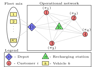
Figure 1: An example network for the SFSMP

There has been a significant quantum of literature on the fleet size and mix problem with electric vehicles when demands and requests are deterministic and constant over the entire planning horizon Golden et al. [1984], Hiermann et al. [2016]. However, to the best of our knowledge, the fleet size and mix literature on urban freight logistics has not considered the uncertainty of operational demand requests in strategic planning.

The contributions of our work are several. First, we propose the SFSMP, a novel stochastic optimization problem for strategic fleet size and mix decision-making in urban freight logistics. Second, we upgrade the state-of-the-art energy consumption model presented by Goeke and Schneider [2015] by explicitly accounting for the energy required for auxiliary usage (such as heating and cooling the cabin space of vehicles, connecting external devices, etc.). Third, we propose a generalization of the Fleet Size and Mix Vehicle Routing Problem (FSMVRP) for the evaluation of the operational problem appearing in the SFSMP that can handle time windows of service, compatibility constraints between vehicles/drivers and customers, driving range limitations, and en-route charging necessities. Fourth, we propose a heuristic variation of the SAA method to solve the SFSMP, where the decision-making in each operational period (both within the strategic decision-making process as well as outside) is carried out using an adaptation of the state-of-the-art Adaptive Large Neighborhood Search (ALNS) algorithm. Finally, we demonstrate the applicability of the approach on two different case-studies of service operations in urban freight logistics.

The remainder of this paper is organized as follows. In Section 2, we present a summary of the literature on fleet sizing problems, urban freight logistics with EVs, energy consumption models, and discuss solution methods in the context of freight logistics planning. A mathematical formulation is presented for the strategic optimization problem with an embedded vehicle routing model for the operational optimization problem in Section 3. We present our adaptation of SAA for solving the SFSMP in Section 4. In Section 5, we present case studies of two Danish organizations embracing electric mobility through research initiatives. We summarize our insights from the analysis of the novel SFSMP and the practical cases in Section 6.

2 Literature Review

Our review focuses on the four major aspects of this paper, namely, fleet size and mix optimization, commercial use of electric vehicles in urban logistics, energy consumption modeling, and relevant methods for solving the problem of interest.

2.1 Fleet size and mix optimization

The fleet size and mix vehicle routing problem (FSMVRP) with deterministic demands that are identical on all operational days accounting for fixed leasing costs and variable routing costs was formalized by Golden et al. [1984]. It was solved using savings based constructive heuristics and a two-phase route first and cluster second algorithm Golden et al. [1984], a generalized assignment based heuristic Gheysens et al. [1984], a matching based tour - fusion heuristic Desrochers and Verhoog [1991], tabu-search based local search methods Taillard [1999], Gendreau et al. [1999], Osman and Salhi [1996], and a sweep-based heuristic method that can also solve non-Euclidean problems Renaud and Boctor [2002]. Baldacci et al. [2009] proposed a two-commodity network formulation of the FSMVRP and presented various valid inequalities to strengthen the formulation.

Liu and Shen [1999] extended this problem to include hard time windows (FSMVRPTW). The FSMVRPTW was solved in the literature using an insertion-based heuristic and an improvement scheme Liu and Shen [1999], a sequential insertion heuristic Dullaert et al. [2002], and a ruin and recreate method Dell’Amico et al. [2007]. More recently, Hiermann et al. [2016] generalized this problem to incorporate driving range constraints of electric vehicles and the option of en-route recharging at the operational level. They solved the problem using an exact branch and price procedure and a hybrid ALNS based heuristic demonstrating the effectiveness of their method on a new set of benchmark instances. The approach of simulation has been used in Cortés et al. [2011] to sample various scenarios to aid in the daily dispatch of technicians.

All the above fleet size and mix problems studied in the literature have considered deterministic customer sets that are known at the strategic planning stage and remain identical through out the strategic planning horizon. Pasha et al. [2016] studied a FSMVRP (without time windows) with deterministic demands that vary on different days. A heuristic method was used to obtain a good common fleet size and mix across the all days after determining the best fleet size and mix independently for each day. Fleet size and mix problems appearing in maritime logistics have considered uncertainty in two-stage stochastic programming problems, such as maintenance operations planning in offshore wind farm management Stålhane et al. [2019] and fleet renewal planning Bakkehaug et al. [2014] under uncertain weather conditions. However, uncertain customer requests at the strategic planning stage have not been considered in the fleet size and mix literature on urban freight logistics so far. In the current paper, we study a fleet size and mix problem in which customer requests are not revealed until the operational period begins.

Fleet sizing boils down to a tradeoff between acquisition costs and operational costs, thus rendering an accurate consideration of the Total Cost of Ownership (TCO) crucial. The TCO of a fleet of vehicles owned by a company must account for various fixed costs (such as capital cost, insurance, and taxes) and variable costs that depend on the duration of operation (such as maintenance and repair costs and energy consumption cost). Rogge et al. [2018] and Schiffer et al. [2018] performed TCO analysis for commercial mixed electric fleets in the context of public transit and mid-haul logistics respectively. In the current paper, we consider a TCO that comprises of one-time purchase costs at the strategic level and energy and maintenance costs that are proportional to the travel time in addition to penalty for not serving some customer in every operational period. A more detailed description of the TCO can also be handled by our mathematical model.

2.2 Urban logistics with electric vehicles

Pelletier et al. [2016] provided an in-depth review of electric vehicle technologies and summarized transportation science literature on goods distribution with EVs. Crainic et al. [2009] presented a brief survey of city logistics problems and discussed models and solution methods for two-tiered city logistics systems. Savelsbergh and Van Woensel [2016] delivered a contemporary perspective of the changing face of city logistics due to the advent of e-commerce prevalence, customer impatience, collaborative consumption, and sustainability consciousness paired with the advancement of digital as well as physical technologies. Tang and Veelenturf [2019] analyze the importance of logistics function in the fourth industrial revolution and offer insights into how the logistics industry can generate economic, environmental, and social value by transforming itself suitably. A common thread revealed in these papers is the need to manage electric vehicles in urban freight logistics. Tracing the beginning of electric VRPs, Conrad and Figliozzi [2011] proposed the recharging VRP and were followed by Erdoğan and Miller-Hooks [2012] with a green vehicle routing problem, and by Schneider et al. [2014] with the EVRP with time windows and recharging stations. The literature in this area has come a long way, with a more recent variant by Cortés-Murcia et al. [2019] allowing alternate modes of transport for customer visits while recharging to reduce loss of productivity. Lin et al. [2016] formulated an electric vehicle routing problem with a heterogeneous fleet that accounts for the impact of speed and vehicle load on battery consumption, allowing en-route charging. Goeke and Schneider [2015] generalized [Schneider et al., 2014] by considering non-linear expressions for fuel and battery consumption and planning with a mixed fleet of EVs and ICEVs. Hiermann et al. [2019] proposed an integrated EVRPTW with a mixed fleet consisting of EVs, plug-in hybrid vehicles, and ICEVs, using constant rates of battery and fuel consumption in their model. Decision-making for green transportation has, in the last decade, helped reducing the negative externalities of freight transport (see Bektaş et al. [2016], Bektaş and Laporte [2011], Bektaş et al. [2018]). We note that the problem of electrification for urban service logistics is significantly relevant given the prevalent interest on adoption of EVs.

2.3 Energy consumption models

Previous works by Erdoğan and Miller-Hooks [2012] and Schneider et al. [2014] considered linear energy consumption functions that were linear in the distance travelled and speed. More advanced energy accounting was performed for ICEVs in Demir et al. [2012]. In their paper, mechanical energy consumption was characterized to overcome rolling resistance, aerodynamic resistance, and gravitational force using expressions that are non-linear in speed. Goeke and Schneider [2015] extended this model to model battery energy consumption of EVs in a load-dependent fashion. Murakami [2017] use this model to present a vehicle routing problem with electric and diesel vehicles with the notion of an original graph for estimating at more accurate road slopes, wait times at road intersections, etc. The existing energy consumption models do not consider the energy consumption due to cabin heating and cooling, which contribute significantly to the reduced driving range during peak winter and peak summer. The power consumed for cabin heating at 0°C and that for cabin cooling at 30°C is around 40% of the total vehicle power for a mid-sized pickup van (seen later in Figure 2). In the current paper, we extend the model in [Goeke and Schneider, 2015] further to include auxiliary energy consumption due to heating and cooling loads and use the non-linear recharging function proposed by Montoya et al. [2017] to determine the time required to charge a given amount of energy. Another aspect in energy consumption calculation of EVs is the effect of battery degradation Pelletier et al. [2017]. We ignore its impact in the current paper.

2.4 Solving the Stochastic Fleet Size and Mix Problem (SFSMP)

The literature on planning problems concerning the strategic and tactical decisions that account for operational efficiency is sparse. Dempster et al. [1981] presented a framework for modeling hierarchical planning problems as multi-stage stochastic programs that are capable of capturing uncertainty at the lower levels of decision-making. More recently, Crainic et al. [2015] considered the tactical planning of the design of the service network in the first tier while accounting for uncertainty in demands in the second tier in a two tier city logistics system. The performance of four tactical plans with associated recourse strategies in the operational stage was evaluated in their paper. To solve two-stage stochastic programs with integer recourse, seminal works have appeared in the literature bringing to the fore various approaches Shapiro et al. [20009] including SAA Ahmed and Shapiro [2002], which was proved to result in a solution that converges to the solution of the original problem as the sample size increases Schultz [1996]. In the current paper, we employ SAA to solve the strategic fleet size and mix problem using the metaheuristic ALNS to solve the operational problem. The metaheuristic method ALNS was first introduced by Pisinger and Ropke [2007] and is considered to be one of the most efficient methods for solving vehicle routing problems with deterministic requests. Other metaheuristics include a genetic algorithm based method Prins [2004] and tabu search methods Gendreau et al. [2008].

In the next section, we present the formulation of the strategic problem as a two-stage stochastic program.

3 Problem Formulation

In this paper, we address the introduction and integration of EVs in a fleet of commercial vehicles operated within urban areas. We consider the vehicles to be used for either cargo pickup and/or service actions (e.g. electric installations, medical visits etc.). The SFSMP is defined as a strategic decision problem. It aims at minimizing the TCO while determining the optimal fleet size and mix for service operations repeating over multiple operational periods. We assume a posteriori customer requests that are not known, owing to the lack of advance information about each day’s requests at the strategic level. However, at the operational level, requests are deterministic. Since strategic decision-making here relies on the trade-off between fleet acquisition cost and average operational cost, an accurate estimation of the operational costs is needed as well.

We formulate the SFSMP as a two-stage stochastic mixed integer program. The strategic horizon consists of a number of operational periods. For example, there may be 1200 days of operation in a strategic horizon of 5 years. The first stage problem is the strategic problem of determining the optimal fleet size and mix that minimizes the sum of the fleet acquisition cost and the expected second stage cost. The strategic decision of the fleet mix is determining the set of vehicles acquired to serve the requirements of the urban logistics operations over the entire horizon in the form of $\bm{w}$, a vector of binary variables such that $w_{k}$ takes a non-zero value if vehicle $k$ of the master list of vehicles $\mathscr{K}$ is acquired. The second stage problem consists of multiple operational periods in which routing decisions of each period are affected by the first stage fleet mix decision only and not the routing decisions of the other periods. In each period of the second stage, only the vehicles chosen for acquisition in the first stage can be used to serve realized customer requests. In every operational period, the operational problem must be solved, which consists in the routing of the drivers, and can be formally defined as a mixed electric fleet vehicle routing problem with time windows and compatibility constraints. We consider a heterogeneous fleet of vehicles of different types varying in size and/or energy source. Although the feasible driving range of most commercial EVs available in the market is typically higher than the distance traversed in urban logistics tours, we allow the possibility of making en-route recharging visits. Additionally, since the duration available for providing service in urban logistics during the day is limited to a daily work shift in a business to business (B2B) service environment, we limit the number of potential visits to recharging stations to one visit. The set of all recharging stations is given by $F$. We remark that adding recharging stops to the routes would result in a loss of productivity even with the latest charging technology in the context of urban logistics and tight time constraints. Each customer request is characterized by a known demand quantity, a hard time window of service, and is associated with a specific level of skill requirement. Without loss of generality, we focus on pickup demands in the case studies that follow. Each driver is assigned a specific skill set that must include the customer’s skill requirement for service to take place. Therefore, we model compatibility constraints between drivers and customer requests. We note that this problem is generic and is capable of handling special cases where all drivers are compatible with all requests.

3.1 First stage problem

The formulation of the first stage problem of the SFSMP is presented with the definition of the sets and parameters presented in LABEL:first_stage. In this stage, the decision variables are binary to indicate whether or not vehicles in the master list should be acquired. Bold notation is used for vector quantities. The vector $\bm{w}$ indicates whether or not each vehicle in the master list of vehicles $\mathscr{K}$ is acquired.

The formulation of the SFSMP is presented below. The strategic objective function accounts for a) the cost of acquiring the vehicles constituting fleet mix configuration determined by the decision vector $\bm{w}$ and b) the total expected operational cost of serving appeared requests with the acquired fleet. The set of acquired vehicles determined by $\bm{w}$ is a subset of the master set of vehicles $\mathcal{K}$. In the expression below, the first term captures the fleet acquisition cost using vehicle acquisition costs $\beta_{k}$ while the second term captures the total expected operational cost summed over $n_{o}$ varieties of operational periods (such as summer, winter, etc.) with $n^{\prime}$ operational periods in each variety. In the second term, $\mathcal{C}(\bm{w},\bm{\lambda},T)$ represents the deterministic operational cost of serving the set of realized customers determined by the vector of random variables $\bm{r}$ (or binary vector $\bm{\lambda}$ of corresponding realized values) at temperature $\mathcal{T}$ which is a random variable (or realized temperature $T$) with fleet determined by$\bm{w}$. Each $\bm{r}^{j},j\in\{1,\dots,n_{o}\}$ represents the binary request vector of customers in the $j$th variety of operational periods. Similarly, $\Omega(\mathcal{T})$ represents the state space of the ambient temperature $\mathcal{T}$ which is a random variable.

$$\min_{\bm{w}}\bigg{\{}\sum\limits_{k\in\mathscr{K}}\beta_{k}w_{k}+\sum\limits_{\bm{r}\in\{\bm{r}^{1},\dots,\bm{r}^{n_{o}}\}}n^{\prime}\ \mathbb{E}_{\bm{r},\mathcal{T}}\left[\mathcal{C}(\bm{w},\bm{r},\mathcal{T})\right]\bigg{\}},$$ (1)

If it is assumed that each operational period faces identical uncertainty in the occurrence of customer requests and ambient temperature, the strategic objective is re-written as (2).

$$\min_{\bm{w}}\bigg{\{}\sum\limits_{k\in\mathscr{K}}\beta_{k}w_{k}+n_{o}n^{\prime}\ \mathbb{E}_{\bm{r},\mathcal{T}}\left[\mathcal{C}(\bm{w},\bm{r},\mathcal{T})\right]\bigg{\}},$$ (2)

where

$$\mathbb{E}_{\mathcal{N},\mathcal{T}}\left[\mathcal{C}(\bm{w},\bm{r},T)\right]=\sum_{\bm{\lambda}\in\{0,1\}^{\mid\mathcal{N}\mid}}\sum_{T\in\Omega(\mathcal{T})}\text{Pr}(\bm{\lambda},T)\ \mathcal{C}(\bm{w},\bm{\lambda},T)$$ (3)

and $\text{Pr}(\bm{\lambda},T)=\text{Pr}(T)\ \prod_{i\in\mathcal{N}}\pi_{i}^{\lambda_{i}}(1-\pi_{i})^{1-\lambda_{i}}$, assuming mutual independence between the occurrence of customer requests and the temperature in the operational period, with the probability of the occurrence of request $i$ given by $\pi_{i}$. In every operational period, a rich vehicle routing problem with deterministic request set determined by $\bm{\lambda}$ and ambient temperature $T$, formulated in the following subsection, must be solved, given that the set of acquired vehicles determined by $\bm{\omega}$. We note that the number of such request sets is exponential in the cardinality of $\Omega(\mathcal{N})$.

3.2 Second stage problem

To complete the model of the SFSMP, the deterministic operational cost $\mathcal{C}(\bm{\omega},\bm{\lambda},T)$ of serving customer set determined by $\bm{\lambda}$ at temperature $T$ with fleet determined by fleet membership vector $\bm{\omega}$ will be defined for all $\bm{\omega}\in\{0,1\}^{\mid\mathscr{K}\mid},\ \forall\ \bm{\lambda}\in\{0,1\}^{\mid\mathcal{N}\mid},\ T\in\Omega(\mathcal{T})$. For ease of exposition, we let $K$ be the subset of vehicles in the master list $\mathscr{K}$ determined by a fleet membership vector $\bm{\omega}$ and we let $N$ be the subset of customers determined by a realized request vector $\bm{\lambda}$. Since the number of available vehicles in each period is fixed, we allow for unserved customers and impose a cost associated with them Lau et al. [2003]. The notation used in this formulation of the operational problem is influenced by that used in the model of Goeke and Schneider [2015] and is presented in LABEL:second_stage and LABEL:dec_var. In this formulation, a network with the set of nodes $N_{0,n+1}^{\prime}$ and the set of arcs $A$ is modeled. The set of nodes includes the set of customers $N$, the set of recharging stations $F$, the source depot node $0$, and the sink depot node $n+1$. A set of acquired vehicles $K$ that contains a set of EVs $K^{E}$ is considered given. For every node $i$, compatibility with drivers $a_{ik}$, demand $d_{i}$ (set to zero at non-customers), time window of service $[e_{i},l_{i}]$, penalty $g_{i}$ for not serving it, and duration of service $s_{i}$ are specified. For every vehicle $k$, driving range in kWh $E_{k}$ (for ICEVs also), daily maintenance and usage cost $f_{k}$, maintenance cost per km $M_{k}$, load capacity $Q_{k}$, average operational speed $v_{k}$, and cost of energy in USD/kWh $c_{k}$ are given. Additionally, $b_{i}(y)$ is a function that calculates the amount of time taken to recharge $y$ units at station $i$. On every arc $(i,j)$, travel time and load-and-temperature-dependent power consumption of vehicle $k$ are given by $t_{ijk}$ and $p_{ijk}(q,T)$ respectively.

Any binary decision variable $x_{ijk}$ takes the value 1 if arc $(i,j)$ is used by vehicle $k$. The binary decision variables $z_{k}$ and $u_{i}$ assume the value 1 if vehicle $k$ is used and if customer $i$ is not served respectively. The continuous variable $y_{ik}$ represents the State of Charge (SOC) of vehicle $k$ upon entering any node $i$ while the variable $Y_{ik}$ is the SOC of vehicle $k$ upon leaving recharging station $i$. The arrival time of vehicle $k$ at each node $i$ is given by $\tau_{ik}$ and the remaining capacity available in vehicle $k$ upon arriving at node $i$ is given by $q_{ik}$.

The objective function (4) minimizes the total fleet operation cost, which is composed of variable energy and maintenance costs, fixed usage costs that can account for acquisition, insurance, maintenance, and driver salaries, and penalties for not serving customers.

Constraints (5) determine the customers that are not served and ensure that all customer nodes are visited at most once. Constraints (6) allow at most one recharging visit on every electric vehicle tour. We add this restriction since the productivity of vehicles and drivers performing intra-day commercial services with short driving duration will take a hit when multiple recharging visits take place during the day. Constraints (7) and (8) ensure flow conservation at the non-depot vertices. Constraints (9) ensures that ICEVs cannot travel to or from recharging stations. This constraint is not included in the formulation of Goeke and Schneider [2015]. We present examples that illustrate the need for this constraint in Appendix B. Constraints (10) determine the vehicles used for operations. Constraints (11) are compatibility constraints, meaning that they deactivate the arcs between incompatible customers and vehicles (drivers). Constraints (12) help determine the service start time at every node on every vehicle while (13) accounts for the time spent in a recharging visit. Constraints (14) ensure that time windows are respected for every node. Additionally, (12)-(14) also serve as sub-tour elimination constraints. Constraints (15) guarantee that the demand of all customers is satisfied without exceeding vehicle capacity. Constraints (16) ensure that the initial cargo level is non-negative and below the vehicle capacity. Constraints (17) compute the SOC at all customer nodes and ensure that it is not negative and does not exceed the battery capacity. Constraint sets (18) and (19) guide the calculation of the SOC post charging, allowing partial recharging while (20) sets the energy range of ICEVs. Finally, the domains of decision variables are defined in (21) and (22). In this formulation, the set $K$ may include EVs and ICEVs with different characteristics of which the subset $K^{E}$ is the set of EVs.

$$\mathcal{C}(\bm{\omega},\bm{\lambda},T)=\min\left[\sum\limits_{k\in K}f_{k}z_{k}+\sum\limits_{(i,j)\in A}\sum\limits_{k\in K}\big{(}c_{k}\ p_{ijk}(q_{jk},T)+M_{k}v_{k}\big{)}\ t_{ijk}\ x_{ijk}+\sum\limits_{i\in N}g_{i}u_{i}\right],$$ (4)

$$\text{subject to: }\sum\limits_{j:(i,j)\in A}\sum\limits_{k\in K}x_{ijk} =1-u_{i} \forall i\in N$$ (5)

$$\sum\limits_{i\in F}\sum\limits_{j:(i,j)\in A}x_{ijk} \leq 1 \forall k\in K^{E}$$ (6)

$$\sum\limits_{j:(i,j)\in A}x_{ijk}-\sum\limits_{j:(j,i)\in A}x_{jik} =0 \forall i\in N^{\prime},k\in K^{E}$$ (7)

$$\sum\limits_{j:(i,j)\in A,\ j\not\in F}x_{ijk}-\sum\limits_{j:(j,i)\in A,\ j\not\in F}x_{jik} =0 \forall i\in N,k\in K\setminus K^{E}$$ (8)

$$x_{ijk}+x_{jik} =0 \forall i\in N_{0},j\in F,k\in K\setminus K^{E}$$ (9)

$$\sum\limits_{j:(0,j)\in A}x_{0,j,k}=\sum\limits_{i:(i,n+1)\in A}x_{i,n+1,k} =z_{k} \forall k\in K$$ (10)

$$\sum\limits_{j:(i,j)\in A}x_{ijk} \leq a_{ik} \forall i\in N,k\in K$$ (11)

$$\tau_{ik}+(s_{i}+t_{ijk})-l_{n+1}(1-x_{ijk}) \leq\tau_{jk} \forall i\in N\cup\{0\},j\in N^{\prime}_{n+1},k\in K$$ (12)

$$\tau_{ik}+t_{ijk}+b_{i}(Y_{ik}-y_{ik})-l_{n+1}(1-x_{ijk}) \leq\tau_{jk} \forall i\in F,j\in N^{\prime}_{n+1},k\in K^{E}$$ (13)

$$e_{i}\leq\tau_{ik} \leq l_{i} \forall i\in N^{\prime}_{0,n+1},k\in K$$ (14)

$$q_{ik}-d_{i}+Q_{k}(1-x_{ijk}) \geq q_{jk} \forall i\in N^{\prime}_{0},j\in N^{\prime}_{n+1},k\in K$$ (15)

$$Q_{k} \geq q_{0k} \forall k\in K$$ (16)

$$y_{ik}-p_{ijk}(q_{jk},T)\ t_{ijk}x_{ijk}+E_{k}(1-x_{ijk}) \geq y_{jk} \forall i\in N,j\in N^{\prime}_{n+1},k\in K$$ (17)

$$Y_{ik}-p_{ijk}(q_{jk},T)t_{ijk}x_{ijk}+E_{k}(1-x_{ijk}) \geq y_{jk} \forall i\in F\cup\{0\},j\in N^{\prime}_{n+1},k\in K^{E}$$ (18)

$$E_{k} \geq Y_{ik} \forall i\in F\cup\{0\},k\in K^{E}$$ (19)

$$E_{k} \geq y_{0k} \forall k\in K\setminus K^{E}$$ (20)

$$x_{ijk},z_{k},u_{i} \in\{0,1\} \forall i,j\in N^{\prime}_{0,n+1},k\in K$$ (21)

$$y_{ik},\tau_{ik},q_{ik},Y_{ik} \geq 0 \forall i\in N^{\prime}_{0,n+1},k\in K$$ (22)

We note that each operational problem is a vehicle routing problem with compatibility constraints (which is NP hard Pillac et al. [2013]) along with capacity and electric range constraints. It becomes intractable to solve the operational problem exactly for realistic customer set sizes. In Section 4, we resort to a state-of-the-art heuristic method, namely ALNS, to solve the operational vehicle routing problem to determine the operational decisions on each day, given a strategic decision $K$. An exact solution of the strategic problem requires solving the operational problem for all possible combinations of fleet mix, ambient temperature, and customer request set. If there is a cap on the total fleet size and/or number of vehicles of each kind in the mix, the number of fleet mix configurations would be finite, albeit numerous. However, it is impossible to enumerate all possible values of $T$ as it belongs to a continuous domain. Even if the temperature domain is discretized, enumerating all possible combinations of the customer set still remains a computationally intensive task. Thus, it is computationally intractable to determine an exact solution of the strategic problem. In Section 4, we propose a novel heuristic solution approach based on Sample Average Approximation (SAA) Ahmed and Shapiro [2002] to circumvent the tedium of exact computation.

3.3 Power consumption model with temperature dependence

We propose an upgraded power consumption model enabling temperature dependence. We account for the following components of power consumption:

• load dependent mechanical power $P_{M}$ (following Bektaş and Laporte [2011], Demir et al. [2011], and Goeke and Schneider [2015]),

• auxiliary power for temperature control $P_{T}$ (heating and air conditioning), and

• auxiliary power usage $P_{O}$.

Ambient temperature has a significant effect on the cabin climate control energy consumption, and extreme temperatures can reduce greatly the range of electric cars. The extent of the impact can be seen through Figure 2, which demonstrates that for a mid-sized van, cabin climate control power is a significant component of the total vehicle power; at -10°C, it is about 4 kW, drawing about 53% of the total vehicle power. The resultant overestimation of driving range by omitting cabin climate control power (auxiliary power) can threaten the feasibility of the implementation of electric mobility in urban logistics operations, and therefore it is important to capture auxiliary power in energy calculations.

Figure 2: Cabin climate control power variation for an electric mid-sized pickup van determined using the upgraded model for a desired cabin temperature of 20 °C: The left side axis tracks the power consumed for cabin climate control while the right side axis captures the climate control power as a percentage of the total power consumed by the vehicle

Our model for the computation of auxiliary power uses the heat balance method as seen in Fayazbakhsh and Bahrami [2013] and Valentina et al. [2014]. The third component of auxiliary power usage refers to the power drawn from the car’s energy source for running an external process such as maintaining a climate control box at a specific temperature in the case of the collection of blood samples from clinics (it excludes the power drawn by music systems and wipers since they depend on a separate 12V battery usually). Including the latter two new components of power has an effect equivalent to boosting all the cost coefficients of $x_{ijk}$’s in (4).

(a) Goeke and Schneider [2015]

(b) Current work

Figure 3: Upgrade to the power consumption model

Power consumption $p_{ijk}(q_{j},T)$ is a function dependent on the starting load at node $j$ and the ambient temperature $T$, when traveling from node $i$ to node $j$ by vehicle $k$. The following expression results in power in kW when using the parameter values indicated in Tables 9, 10 and 11 in the appendix.

$$p_{ijk}(q_{j},T) =\begin{cases}\phi^{d}\varphi^{d}P_{ijk}(q_{j},T)&P_{ijk}(q_{j},T)\geq 0,k\in K^{E}\\ \phi^{r}\varphi^{r}P_{ijk}(q_{j},T)&P_{ijk}(q_{j},T)<0,k\in K^{E}\\ \max\left(kN^{\prime}D+\frac{P_{ijk}(q_{j})}{\eta^{\prime}\cdot\eta_{tf}},0\right)&k\not\in K^{E}\end{cases}$$

$$P_{ijk}(q_{j},T) =P_{M}((i,j),k)+P_{T}((i,j),k,T)+P_{O}$$

$$P_{M}((i,j),k) =0.001\times\left[c_{r}m_{k}(q_{j})g\cos\alpha+\frac{1}{2}\rho_{a}A_{f}c_{d}v^{2}+m_{k}(q_{j})g\sin\alpha+m_{k}(q_{j})a\right]v$$

$$P_{T}((i,j),k,T) =\mathcal{I}_{H}\frac{1}{\eta_{H}}(P_{H}+P_{Con})+\mathcal{I}_{C}\frac{1}{\eta_{C}}(P_{C}+P_{Con}+P_{Rad}+P_{P}),$$

where $P_{M}((i,j),k)$, $P_{T}((i,j),k,T)$, and $P_{O}$ are mechanical, temperature control, and auxiliary power usage components respectively. The terms $\mathcal{I}_{H}$ and $\mathcal{I}_{C}$ are binary variables that indicate whether the heating mode or the cooling mode is being used in the definition of $P_{T}$. The components of $P_{T}$ are further defined below.

$$P_{H} = \dot{m}\ C_{P}\ (T_{d}-T)$$

$$P_{C} = \dot{m}\ C_{P}\ (T-T_{d})$$

$$P_{Con} = \sum_{i\in Surfaces}A_{i}U_{i}\lvert T-T_{d}\rvert$$

$$P_{Rad} = \sum_{i\in Surfaces}A_{i}\tau_{i}{I}_{DN}\bigg{(}\cos\theta_{i}+C\frac{(1+\cos\Sigma)}{2}+\rho_{g}\cos\theta_{z}\frac{(1-\cos\Sigma)}{2}\bigg{)},$$

$$\text{where }I_{DN} = A\exp(-B/\cos\theta_{z})$$

$$P_{P} = \sum_{i\in Persons}H_{Pr}A_{Du}$$

The main component is the ventilation load, i.e., the power required to warm up ($P_{H}$) or cool down ($P_{C}$) the air entering the car. The rest of components are the following: $P_{Con}$ is the power loss due to conduction through the surfaces of the vehicle and/or exterior and interior convection, $P_{Rad}$ represents the cooling load introduced in the car due to direct and diffuse solar radiation, and $P_{P}$ is the cooling load corresponding to the metabolic heat generated by humans seated in the vehicle. A brief description of all the parameters along with pointers to their sources is presented in tables 9, 10 and 11 in the appendix. Specifically, the efficiency parameters used in the definition of $p_{ijk}(q_{j},T_{o})$ are defined in Table 9, and the parameters used in the definitions of $P_{M}$ and $P_{T}$ are defined in Table 10 and Table 11, respectively.

4 Methodology

Since the SFSMP is a two-stage stochastic program, we employ a fairly standard method, known as Sample Average Approximation (SAA), used in the literature for pursuing solutions of two-stage stochastic programs. We propose solving the SFSMP by SAA through Monte Carlo sampling of the requests and ambient temperature using known probability distributions.

4.1 Solving the strategic problem

We propose a nested framework of solving the fleet sizing problem with lack of knowledge on the occurrence of demand requests and daily temperatures at the strategic level. The framework is is delineated through a flow chart in Figure 3. For every initial fleet mix, the set of customer requests and the ambient temperature are sampled. On the resultant operational instance, the ALNS algorithm is applied to determine the operational cost for each sample instance $i$, which is $\mathcal{C}(\bm{\omega},,\bm{\lambda}^{i},T^{i})$. The half width of the confidence interval for the sample average estimate based on the samples generated so far is determined. If it meets the required criterion (for e.g., of falling under a certain threshold), the process proceeds to computing the sample average operational cost for the considered fleet mix. In this step, we approximate the expectation in (2) with a sample average of costs of operation.

$$\mathbb{E}_{\mathcal{N},\mathcal{T}}\left[\mathcal{C}(\bm{\omega},\bm{r},\mathcal{T})\right]\approx\frac{1}{n}\sum_{i=1}^{n}\mathcal{C}(\bm{\omega},\bm{\lambda}^{i},T^{i}),$$ (23)

where $n$ is the number of samples with the simulated outcomes of customer set determined by $\bm{\lambda}^{i}$ and ambient temperature $T^{i}$, for each operational period $i$. After evaluating the sample average operational cost for all the fleet mixes of interest, the best fleet mix is determined.

We remark that an exhaustive enumeration of fleet mixes may result in an exponentially large number of fleet mixes if the master list of vehicles is heterogeneous and large. Thus, it is suggested that the set of fleet mixes may be determined heuristically or exhaustively, depending on the size of the problem. Given the list of preferred commercial vehicles for inclusion in the fleet, enumeration with reasonable step sizes would be practical.

Figure 4: Solving the Stochastic Fleet Size and Mix Problem (SFSMP) using Sample Average Approximation (SAA)

4.2 Solving the operational problem

In this section, we present the solution method used to determine decisions that must be implemented in each period of operation. Since determining an exact solution of the operational problem presented in Section 3 is not computationally tractable for realistically sized instances, we pursue a heuristic approach. In particular, we develop a ALNS algorithm (Røpke and Pisinger [2006]), which has been utilized extensively in the literature to solve vehicle routing problems and specifically, the mixed fleet vehicle routing problem with time windows, as can be seen in Goeke and Schneider [2015] and Keskin and Çatay [2016]. We use the same parameters as those used in [Christensen, 2014].

We have employed the following destroy operators for customer removal in the algorithm:

1. Random removal [Røpke and Pisinger, 2006]: A given number of randomly chosen customers are removed from the tours.

2. Worst removal [Røpke and Pisinger, 2006]: A given number of customers that result in the highest insertion costs are removed.

3. Shaw removal [Røpke and Pisinger, 2006]: A given number of customers related to each other through a randomly selected initial customer according to five different criteria (customer proximity, tour proximity, demand difference, arrival time difference and time window similarity) are removed.

4. Random route removal: Entire tours are removed from a given solution until a given number of customers are removed.

5. Slack Induced String Removal (SISR) [Christiaens and Vanden Berghe, 2018]: This destroy operator was introduced in [Christiaens and Vanden Berghe, 2018]. Strings of nodes or pairs of strings of nodes separated by a few nodes are removed.

The following repair methods have been used for inserting the removed customers:

1. Greedy insertion [Røpke and Pisinger, 2006]: The customer node to be inserted and the position of insertion are determined by minimizing the cost of insertion among all feasible insertions.

2. 2-Regret insertion [Røpke and Pisinger, 2006]: In this repair method, we select the customer for which the difference between the second lowest insertion cost and the lowest insertion cost is maximum. This customer is then inserted in its best position.

The insertion methods are modified to allow at most one recharging visit on each tour. In this ALNS, a simulated annealing based acceptance criterion is employed to guide the search. The start temperature is calculated such that a solution $s$ times worse than the starting solution is accepted with a probability of 50%, in the first iteration.

$$T_{Start}=-\frac{sf(x)}{\text{ln}(0.5)}$$

Additionally, a resetting mechanism is used to refresh the current solution with the best solution after a certain number ($\gamma$) of iterations without any improvement to the best solution. We present the other parameters used in the ALNS in Table 7 of Appendix A.

5 Case Studies

As part of the EU-funded research project called Electric Urban Freight and Logistics (EUFAL), the aim of which is to encourage the electrification of commercial fleets in order to reduce the carbon footprint of urban logistics operations, we developed two real case studies. We present our analysis of the two cases in this section.

5.1 Blood sample collection from private clinics for Region Hovedstaden

Region Hovedstaden (Region H: www.regionh.dk/) is a public authority that manages healthcare and social services in the Capital Region of Denmark, which corresponds roughly to the metropolitan area of Copenhagen. Collecting blood samples from doctors and delivering these to a testing facility is one of the functions carried out by the Region, which is the focal logistics process of this case study. Everyday, blood samples must be collected from the clinics of private physicians and delivered to the laboratory testing facility in a hospital by vehicles that start their trips from a different hospital that is about four kilometers away from the first hospital. Due to the perishability of the collected samples, a 150 minute shift is designed for all drivers. Since the viability of the samples degrades beyond three hours after extraction, physicians would be able to send the samples by taxi if the fleet operation plan does not pick up from the corresponding physician location. On each work day, the Region operates two identical blood sample collection shifts - one in the forenoon and one in the afternoon. The Region aims to optimize its mix of delivery fleet and make smart operational decisions to minimize the cost of missed doctor visits and the cost of energy used for routing. We consider the problem of strategic sizing of the fleet required to manage these operations. Similar operational problems were considered by Grasas et al. [2014] in Catalonia, Zufferey et al. [2016] in Geneva, and Anaya-Arenas et al. [2014] and Kergosien et al. [2014] in Quebec.

In line with its mission, the Region plans to use an all-electric fleet for its logistics operations. It has access to two different types of vehicles, medium-sized electric pickup vans and electric cargo bikes with driving ranges of 270 and 140 kilometers respectively. The characteristic parameters of the two types of vehicles considered in this study are presented in Table 4 and are inspired from those of the mid-sized electric pickup van Renault Kangoo and the electric cargo bike TRIPL. Though the cargo bike does not have to manage cabin climate control, the climate box used for maintaining the temperature of the collected blood samples at 20 degree Celsius draws energy from its battery directly with a base power of 0.1 kW in addition to the actual power required to heat or cool the box. In the electric van, the climate box is hooked to its secondary 12V battery, thus not affecting the driving range of the vehicle.

Table 4: Region H case: Features of the vehicles considered

Feature	Pickup Van	Cargo bike
Kerb weight	1426 kg	322 kg
Max speed	130 kmph	45 kmph
Operational speed	45 kmph	40 kmph
Battery	33 kWh	8.64 kWh
Capacity	720 vials	288 vials
Additional weight	200 kg	50 kg
Acquisition cost	28,223 USD	17,900 USD
Auxiliary power	0	0.1 kW

The Region is now faced with the decision of determining the number of vehicles of each type required to constitute its fleet for its long term operations. At the operational level, the requests from doctors are revealed on the day of operation. However, the actual demands are not known days in advance. Based on data collected through a survey we conducted, we found that the demands are seasonal and can be assumed to follow different distributions in summer and non-summer parts of the year. A detailed description of the generation of operational instances for this case study may be seen in Appendix C. Based on initial experiments, we have found that the maximum fleet size will never exceed $15$. Thus, we consider all vehicle mix possibilities such that the total fleet size does not exceed $15$. A horizon of 10.6 years with 227 working days per year and two work shifts per day is considered as the horizon based on the average lifetime of vehicles stated in Mitropoulos et al. [2017]. For every possible fleet mix, an estimate of the operational cost is determined over the entire horizon. To this estimate, the acquisition cost of the corresponding fleet mix is added to determine the TCO. The best fleet mix is thus determined using the procedure described in Figure 4. Since we adopt SAA to solve the SFSMP, the approximation of the expected cost relies on a sample average, for computing which, choosing the right sample size is crucial. Figure 5 presents an analysis of the variation of the half width of the 95% confidence interval of the average routing cost for two fleet mixes at various sample sizes. We note that the half width stabilizes beyond 500 samples. However, considering the average number of unserved customers (or equivalently, the average cost of missing customers), we note that 600 or more samples would be required for the [0 vans, 5 cargo bikes] fleet mix. However, there are no unserved customers for the other mix. Considering both these aspects, 600 samples for the former and 500 samples for the latter mix would be sufficient to obtain a meaningful sample average. It is clear that the required sample size depends on the actual configuration considered and that the solutions of interest have a sample size requirement under 1000 samples. To obtain the following results, we use 1000 samples for all the fleet mixes.

Figure 5: Region H case: Half width analysis for the fleet mix containing [0 vans, 5 cargo bikes] and [1 van, 5 cargo bikes]

The fleet mix, the TCO, and the average fill rate of the ten best heuristic solutions that minimize the TCO of the fleet are presented in Figure 6. We note that the tenth best solution to the stochastic problem is about $40,000$ US dollars costlier than the first best solution. Such a difference (25% of the first best solution’s TCO) reaffirms the need to incorporate the impact of uncertainty into the study. The composition of the fleet mixes of the top ten solutions indicate that there is a strong preference for the inclusion of cargo bikes in the mix and that pickup vans, though not as popular, do appear in six positions. It may be noted that broadly, a pickup van is equivalent to (and slightly more expensive than) two cargo bikes in the marginal sense. We note that in spite of the variation of the fleet mixes, the average capacity fill rates of nine of the ten solutions fall in the 50-80% range.

Figure 6: Region H case: The ten best fleet mix solutions determined by SAA with their composition, TCO, and average fill rates

The best fleet mixes optimize for a given demand characterization, leaving little room for planned redundancy. While operating logistics systems, planners prefer adding a safety factor to build in resilience against near-future changes due to the overall evolution of the system. In Figure 7, we present a plot of the variation of TCOs with increasing level of demand scaling. The base case of the scaling factor set to 1 is the current demand situation faced by the Region. The remaining factors scale down or up the demand faced at every clinic. We note that the best mix [1 van, 4 cargo bikes] remains a preferred solution for the interval [0.95, 1.15] of the scaling factor. However, when planning for scenarios with scaling between [1.2, 1.3], the mix [1 van, 5 cargo bikes] is preferred. We find that at higher TCOs, there is greater safety against fluctuations in demand levels. Although these levels of variation in demand may not seem very realistic for the current case study, this analysis would be applicable to other case studies dealing with different products. Thus, a firm planning to add in redundancy into its fleet management may seek a fleet mix with higher TCO to ensure readiness for overall higher demand scenarios.

Figure 7: Region H case: Sensitivity analysis of the top eight fleet mix solutions to variation of scaling demand at all clinics. In the legend, an entry with $[a,b]$ refers to the fleet mix with $a$ vans and $b$ cargo bikes.

Figure 8 presents the variation of average operational cost for the best fleet mix [1,4] in response to a variation of temperature. We note that sub-zero temperatures lead to a higher overall energy consumption compared to tropical temperatures. At $0$ degrees Celsius, not including the effect of temperature on vehicular power consumption leads to a 20% difference from the base case (of 20 degree Celsius since the desired cabin temperature is 20 degrees Celsius) where the effect of temperature is not considered. This affects the service plan critically resulting in the mismanagement of the logistics system, since the available energy reserve as well as the driving range are overestimated during planning if the effect of cabin climate control and auxiliary energy usage are not considered.

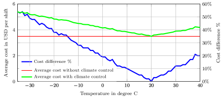
Figure 8: Region H case: Average operational cost per shift in USD (left axis) and percentage cost difference over the case of no cabin climate control (right axis) with varying ambient temperature for the best fleet mix solution with 1 van and 4 cargo bikes

Thus, the case study of the Region Hovedstaden reveals important insights regarding the importance of modeling uncertainty, the sensitivity of solutions to variations in demand levels, and the effect of temperature on planning fleet operations.

5.2 Technician routing for MT Højgaard

In this case, a Danish construction company, MT Højgaard (MTH), is currently considering electrification of the commercial fleet of its subsidiary Lindpro, provided there is no negative impact on their business performance. Lindpro is an electric installations company that provides electrician services to various customer locations. Each technician has a specific skill level and technicians with higher skill levels are capable of attending to tasks of skill levels lower than their skill level. However, in reality, the company allows technicians of a specific skill level serving at most one level below their skill level. The company currently operates small and large ICEVs in its fleet. In this case study, we consider the strategic decision of investment in the fleet (as if the entire fleet must be acquired now). Only the small ICEVs are currently being considered for replacement with EVs as the tasks and routes operated by the large ICEVs are not yet relevant for replacement with EVs. Each driver begins and ends his/her tour at their homes.

Villegas et al. [2018] considered a technician routing problem with mixed electric fleet and proposed a decomposition based solution method. We endeavor to determine the fleet mix using SAA. The ALNS is modified to allow compulsory visits to a driver’s home at the start and end of their tours if the corresponding vehicle is used.

We generated a master list of customers in the Greater Copenhagen region with potential tasks that are associated with service times, time windows, and skill requirements inspired from historical information. Compatibility matrices were developed with the following rules based on discussions with MTH:

• There are four skill levels that enable matching customer requests and technicians, where Level 1 is the most basic (handyman) while Level 4 is specialty (classified technician).

• Technicians of a particular skill level step down by at most one level.

• It is fairly common for technician of a certain level to perform tasks one level below. However, it is very rare for Level 2 technicians to perform Level 1 tasks since Level 1 technicians belong to a union that is different from that of technicians of other levels.

A detailed description of the various aspects of sample instance generation is provided in Appendix D.

Figure 9: MTH case: Half width analysis for the fleet mix containing 5 and 25 EVs

As part of implementing SAA, we determined the suitable sample size based on the stabilization of the half width of the 95% confidence interval of the sample average of the operational cost (see Figure 9). We found that a sample size of 200 would be sufficient.

Table 5: MTH case: Features of the vehicles considered

Feature	EV	Small ICEV	ICEV
Kerb weight	1430 kg	1623 kg	1800 kg
Operational speed	43.2 kmph	43.2 kmph	43.2 kmph
Battery	33 kWh	-	-
Additional weight	250 kg	250 kg	400 kg
Acquisition cost (USD)	32,000 USD	21,000 USD	28,000 USD
Auxiliary power	0	0	0

The features including the additional load carried as electrician equipment in the vehicles are presented in Table 5. Since the 44 small vehicles can be either ICEVs or EVs, we considered fleet mixes with 0, 5, $\dots$, 44 EVs and with the remaining small vehicles being ICEVs. When 5 EVs are included in the fleet, the first 5 drivers out of the 44 drivers are assigned EVs. The list of drivers is in the order of the drivers’ EV eligibility, which is determined by the proximity of their home addresses to the nearest charging stations (see Appendix D). On solving the ALNS for each of these fleet mixes for each of the sample days, we determine the average daily operational cost (see the upper plot of Figure 11), which reduces with increasing number of EVs in the fleet. The ALNS also generates the tours that must be executed on each day. Table 6 presents some statistics pertaining to prescribed tours by vehicle type. On average the EVs in the fleet spend greater duration driving compared to the ICEVs. Correspondingly, the average task time (also considering breaks as tasks) of EVs is also more than an hour lower than that of ICEVs operated in the fleet. Thus, EVs are deployed to perform less time-consuming tasks and drive between customer locations more often since the energy consumed in driving EVs is cheaper than that for ICEVs. In spite of the longer duration spent on driving around, the average amount of energy consumed by EVs is 5.6 kWh based on results from 200 sample days. Though the planned energy usage of EVs very rarely exceeds 16 kWh on any tour, there are two occurrences when the SOC at the end of the tour drops below 6% of the usable battery capacity of 30 kWh, 24 occurrences when it drops below 20%, and 148 occurrences when it drops below 30%. These occurrences usually take place under 1 °C. Figure 10 presents a measure of range anxiety, i.e., the temperature-dependent risk of the SOC falling below 25% and between 25-35% of the battery capacity in terms of the number of times it happens in 200 sample days with 110,786 prescribed tours. We note that at low temperature, drivers run a significantly high risk of facing range anxiety. This observation indicates that if the power consumption model had not accounted for temperature-dependent power, such a prescription of tours would result in en-route driving range chaos.

Table 6: MTH case: Tour statistics by vehicle type

Vehicle	Customers served	Driving time (h)	Serving time (h)	Avg. task time (h)	Tour cost (USD)
EV	7.86	1.05	8.47	1.54	2.77
Small ICEV	4.11	0.42	8.52	2.70	2.31
ICEV	3.68	0.57	8.19	2.97	3.23

Figure 10: MTH case: A stacked histogram (left axis) presents the frequency of occurrence of EV tours in which the SOC at the end of the tour falls between 25-35% (pink) and below 25% (red) based on computational results from 200 sample days with 110,786 EV tours. The probability density function (a relative measure obtained by summing over the probability densities of four seasons) of temperature is presented in black (right axis).

We then computed the TCO of the fleet using existing retail prices presented in Table 5 (excluding value added tax, green incentives, etc.) and we plotted it in red in the lower part of Figure 11. We note that without any additional taxes and incentives, it is not preferred to include any EVs in the fleet (comparing against the black line that indicates the TCO of the fleet containing no EVs).

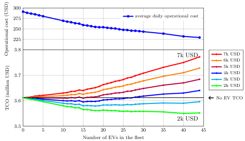
Figure 11: MTH case: (a) Variation of average daily operational cost and (b) Variation of TCO with EV composition at various levels of price difference between EV and small ICEV when the small ICEV’s price is fixed at 21k USD, the price of diesel is 1.34 USD/liter, and the price of electricity is 0.1973 USD/kWh.

We vary the price difference between the two competing classes of vehicles, namely small ICEVs and EVs, by fixing the retail price of the former at 21k USD (where 1k = 1,000) and varying the price of the latter above 21k USD in Figure 11. We note that EVs begin to become favorable only when the price difference drops below 5k USD. When the price difference falls below 3k USD, it is profitable to make all the small vehicles EVs. We note that significantly high savings are made by the firm by owning 44 EVs in the long run to the tune of 50k USD over owning 44 small ICEVs, when the price difference drops to 1000 USD.

(a) 1.23 USD

(b) 1.43 USD

(c) 1.63 USD

(d) 1.83 USD

Figure 12: MTH case: Sensitivity of the tendency of EV inclusion in the fleet to variation in electricity and diesel prices at various levels of price difference between EV and small ICEV: The number of EVs out of 44 small vehicles in the fleet up to which TCO is lower than that of a no-EV fleet mix is indicated.

Figure 13: MTH case: Variation of the number of EVs in the fleet in response to variation in diesel and electricity prices when EVs are 5k USD more expensive than ICEVs

Since the operational costs are heavily dependent on the prices of diesel and electricity, based on corresponding TCOs, we performed an analysis of the variation of the EVs composition in the fleet with variation in diesel prices between 1.23-1.83 USD/liter and electricity prices between 0.16-0.32 USD/kWh. Figure 12 presents the number of EVs to be included in the fleet profitably at various levels of price difference between the competing vehicle classes. Confirming our intuition, we find that at lower electricity prices and higher diesel prices, there is an increased preference for the inclusion of EVs in the fleet. However, at the current retail price difference of 11k USD, it is not profitable to include EVs in the fleet for any reasonable combination of energy prices. Thus, additional incentives are necessary to encourage commercial EVs ownership. When the effective price difference is between 7k-3k USD, various partial EV fleet mixes are optimal. Under a price difference of 2k USD, all the small vehicles will be made EVs for almost all the energy price combinations. For a price difference of 5k USD, we present the variation of the tendency of electrification with the variation of energy source prices in Figure 13. As expected, lower electricity prices and higher diesel prices favor EV strength in the fleet.

Figure 14: MTH case: Variation of the average operational cost the fleet in response to variation of additional mass levels when temperature is fixed at 0 degree Celsius. In the upper plot, the maximum difference in TCO for various fleet sizes is presented. TCO_i is the TCO computed at additional mass level $i$.

Next, we vary the additional load carried in all the vehicles through seven levels $1,\dots,6$, where the load mass is the level multiplied by 100 kg for EVs and small ICEVs while it is the level multiplied by 200 kg for the larger ICEVs (since the maximum allowed load for small and large vehicles is 600kg and 1200kg respectively). For these experiments, the ambient temperature is fixed at 0 degree Celsius. From Figure 14, we note that the average operational cost is affected by the additional mass level inasmuch as leading to 9% difference between the highest and lowest additional mass levels. The corresponding difference in TCO is to the tune of 50-65k USD. Thus, we note that it is necessary to account for the additional mass carried by commercial vehicles while planning their operations.

The solution method presented in this paper will serve as a useful tool to policy-makers in determining effective incentive schemes as well as to firms to determine the profitable extent of EV ownership.

6 Conclusion

So far, fleet size and mix vehicle routing problems have not considered uncertainty of operational scenarios at the strategic decision stage. We fill this gap by proposing a novel two-stage stochastic program problem framework SFSMP and solving it by SAA through the use of the metaheuristic method ALNS for operational cost determination and decision-making. From a modeling perspective, other recourse decisions, such as renting out acquired vehicles when idle or receiving chartered services when needed, may be investigated in future research. Also, the timing for selling acquired vehicles and the corresponding salvage values may be included in future work. Additionally, other solution methods may be explored to tackle the strategic as well as operational decision stages.

In addition to presenting a novel problem, we evaluate the total cost of ownership of a mixed fleet with electric vehicles through two Danish case studies. The cases confirm the importance of considering the uncertainty in requests at the strategic planning stage and including cabin climate control power and auxiliary power in the computation of vehicle power for planning purposes. Additionally, the versatility of the proposed approach to not only determine the best fleet mix but also assess the robustness of the prescribed solution is demonstrated. We note that although we consider electric vehicles in this paper, other alternate sources of renewable energy (hydrogen-based, etc.) may be considered instead to understand their potential.

Appendix A Parameters

Table 7: Parameters used in the ALNS Christensen [2014]

ALNS Røpke and Pisinger [2006]
Notation	Description	Value
$\zeta$	cooling factor	0.9999
$\omega$	start temperature parameter	0.015
$\pi$	maximum removal percentage	35%
$\pi^{\prime}$	minimum removal percentage	5%
$\eta$	segment size	125
$\gamma$	resetting parameter	5000
$r$	reaction factor	0.1
$\sigma_{1}$	new global best reward	33
$\sigma_{2}$	better current solution reward	9
$\sigma_{3}$	new solution reward	13
Worst removalRøpke and Pisinger [2006]
$p_{worst}$	probability factor	4
Shaw removalRøpke and Pisinger [2006]
$\varphi$	distance weight	9
$\chi$	time weight	3
$\psi$	demand weight	2
$\omega$	same route weight	5
$p_{shaw}$	probability factor	4
SISR Christiaens and Vanden Berghe [2018]
$\overline{c}$	average number of removed customers	10
$L_{\max}$	maximum cardinality of removed strings	10
$\alpha$	probability of not increasing the preserved string size	0.01
$\beta$	blink rate	0

Table 8: Parameters for costs by vehicle type

EVs
Notation	Description	Value	Source
$f_{k}$	usage cost in USD	0
$c_{k}$	energy cost in USD per kWh	0.1973 for EV, 0.2021 for ICEV	Avg. diesel price is 1.34 USD per liter
$M_{k}$	maintenance cost in USD per km	0.080837 for electric vans, 0.017015 for electric cargo bikes, and 0.115481 for ICEVs	Mitropoulos et al. [2017]

Table 9: Parameters for efficiency by vehicle type

EVs
Notation	Description	Value	Source
$\phi^{d}$, $\phi^{r}$	electric engine efficiency during discharge and recuperation	1.184692, 0.846055	Goeke and Schneider [2015]
$\varphi^{d}$, $\varphi^{r}$	coefficient to account for external factors and SOC for discharge and recuperation	1.112434, 0.928465	Goeke and Schneider [2015]
ICEVs
Notation	Description	Value	Source
$k$	engine friction factor	0.2 kJ / rev / l	Demir et al. [2011]
$N^{\prime}$	engine speed	33 rev/s	Demir et al. [2011]
$D$	engine displacement	1.6 liters	Renault Danmark [2018]
$\eta^{\prime}$	efficiency parameter for diesel engines	0.9	Demir et al. [2011]
$\eta_{tf}$	drive train efficiency	0.4	Demir et al. [2011]

Table 10: Parameters for $P_{M}$ in the energy consumption model

$\bm{P_{M}}$
Notation	Description	Value	Source
$c_{r}$	coefficient of rolling friction	0.01	Demir et al. [2011]
$\alpha$	gradient of the road	0°	Case study specific.
$\rho_{a}$	density of air	$1.2041$ kg/m3	Demir et al. [2011]
$A_{f}$	frontal surface area of the vehicle	$4.06$ m2	Kühlwein [2016]
$c_{d}$	drag coefficient	$0.34$	Kühlwein [2016]
$m_{k}(q_{j})$	total mass due to vehicle in kg $k$ with mass $q_{j}$ reaching node $j$	-	Case study specific.
$g$	gravity acceleration	$9.81$ m/s2	Demir et al. [2011]
$v_{k}$	average speed of vehicle $k$ in m/s	$12$ m/s	-
$a_{k}$	acceleration of vehicle $k$ in m/s2	0.01 m/s 2	Demir et al. [2011]

Table 11: Parameters for $P_{T}$ in the energy consumption model

$\bm{P_{T}}$
Notation	Description	Value	Source
$A$, $B$, $C$	constant coefficients from ASHRAE Clear Day Solar Flux Model	1.088, 0.205, 0.134	Ramsey and Kuehn [2018]
$\theta_{z}$	zenith angle (the angle of solar light with respect to the vertical)	35o	EUNADICS-AV [2018]
$\theta_{i}$	angle of incidence (with respect to the normal to surface $i$)	55o	EUNADICS-AV [2018]
$\rho_{g}$	reflectivity of ground	$0.2$	Fayazbakhsh and Bahrami [2013]
$A_{i}$	area of surface $i$	$A_{\text{windshield}}=1$ m2, $A_{\text{window}}=0.6$ m2, $A_{\text{rear}}=0.8$ m2, $A_{\text{roof}}=1$ m2, $\sum_{i}A_{i}=4$ m2	Fayazbakhsh and Bahrami [2013]
$\tau_{i}$	emissivity of surface $i$	$0.8$	Fayazbakhsh and Bahrami [2013]
$U_{i}$	heat transfer coefficient of air with respect to surface $i$	$0.003$ kW/m${}^{2}\cdot$K	Fayazbakhsh and Bahrami [2013]
$C_{P}$	specific heat of air at constant pressure	$1.005$ kJ/kg$\cdot$K	Fayazbakhsh and Bahrami [2013]
$\eta_{H/C}$	thermal efficiency of heaters or coolers	$2.5$ for both	Liu et al. [2018]
$\dot{m}$	mass of air flow rate from the heater/cooler	$0.3185$ kg/s	Song et al. [2015]
$H_{P}$	human heat production rate	$58.2$ W/m2	Fayazbakhsh and Bahrami [2013]
$n_{p}$	number of passengers	$1$	-
$A_{Du}$	DuBois area (the surface area of skin of an adult)	$1.8$ m2	Fayazbakhsh and Bahrami [2013]
$T_{d}$	desired temperature	20°C	-
$T_{o}$	outside temperature	-	See Section 5

A.1 Parameters for the recharging functions from Montoya et al. [2017]

$$\text{30kWh Standard \acs{SOC} in kWh}=\begin{cases}0.1828t&0\leq t\leq 139.5\text{ min}\\ 0.08889t+13.1&139.5\leq 173.25\text{ min}\\ 0.02778t+23.6875&173.25\leq t\leq 227.25\text{ min}\end{cases}$$

$$\text{30kWh Fast \acs{SOC} in kWh}=\begin{cases}0.83089t&0\leq t\leq 30.69\text{ min}\\ 0.40404t+13.1&30.69\leq 38.115\text{ min}\\ 0.12626t+23.6875&38.115\leq t\leq 49.995\text{ min}\end{cases}$$

Appendix B Clarification for constraint (9)

In the model of Goeke and Schneider [2015], there are no constraints enforcing that ICEVs cannot travel to or from recharging stations. In Figure 15 two feasible solutions for an ICEV, $k$ is shown. These two examples show how omitting constraint (9) can lead to undesired solutions.

(a) Time can be reset to 0

(b) Flow constraints can be circumvented

Figure 15: Examples of undesired solution, feasible in the model of Goeke and Schneider [2015]

Figure 15(a) shows an example where the time variable can be reset to 0. Constraint (12) is not posted for arcs leaving an recharging station, and therefore the only thing constraining the $\tau$ variable at the customer nodes is the non-negativity constraint (22). This is obviously a problem as we are working with time-windows. In Figure 15(a) the route alternates between a recharging station and a customer node. That is to satisfy the flow conservation constraint (8). The left hand side of (8) does not account for arcs with an end node being a recharging station. Therefore, for all nodes in Equation 8 both summation of the left hand side will be equal to $0$.

Figure 15(b) shows an example where the flow of an ICEV can consist of multiple weakly connected components. Here one component is an actual route starting at the depot and visiting customers $a,b,c,d$, and $e$ before returning to the depot. Another component is the subgraph composed of the nodes $f$ and $g$ in addition to the arc $(f,g)$. As previously described, the flow conservation constraint (8) does not account for the arc $(f,g)$, as it originates at a recharging node. Furthermore, the flow conservation constraint is not posted for recharging nodes, making the overall flow feasible for an ICEV.

To disallow these solutions we have included constraint (9) in the model.

Appendix C Instance generation for the Region H case

1. Number of customers: Based on the data from Region H, we created a truncated normal distribution whose output is rounded to the closest integer. It has the following parameters:

   • Mean = 107.8946,

   • Standard deviation = 26.63986, and

   • Truncation (lowest: 26.5, highest: 145.5).

2. Taxi cost: The average cost of taxi trips is estimated to be 30 USD since a taxi trip in Copenhagen costs around 30 USD for 8km, which is twice the distance from Bispebjerg Hospital to Frederiksberg Hospital, based on information from the DanTaxi website
   (https://dantaxi4x48.dk/hvad-koster-en-taxa/).

3. Temperature: We calibrated four triangular distributions, one for each season, based on data in degrees Celsius from the Danish Meteorological Institute (dmi.dk). Each season has a 25% probability of being selected.

   Table 12: Description of seasonal triangular distributions of temperature

   	Minimum	Maximum	Mean
   Summer	13.4	26.9	19.5
   Autumn	1.2	21.8	10.7
   Winter	-7.3	8.8	2.3
   Spring	-4	24.1	8.2

4. List of customers’ locations: Each clinic has a certain probability of being selected, which was calculated from the historical data provided by Region H. Addresses of the clinics were provided by Region H (also available publicly) and were geocoded using the tool provided at the website https://geocode.localfocus.nl/.

5. Customer time windows and service times: We obtained the time windows and service times (of 3 minutes per clinic) for various clinics based on data provided by Region H.

6. Demands: Based on an online survey conducted by us, we calculated the average number of vials handled by a doctor depending on the day of the week and on whether it is summer (lower due to vacation) or the rest of the year, so in total we calculated 10 averages (summer Monday, rest of the year (ROTY) Monday, summer Tuesday, etc.). We rounded those averages to the closest integer and multiplied them by the number of doctors in each clinic to obtain the demand per clinic. The days of the week were selected with a 20% probability each while summer was selected with a 25% probability.

   Table 13: Demand quantity per doctor per day by season (in number of vials)

   Summer	Monday	Tuesday	Wednesday	Thursday	Friday
   	6	6	4	6	5
   ROTY	Monday	Tuesday	Wednesday	Thursday	Friday
   	9	8	6	7	6

7. Travel times: Free flow travel times between origin-destination pairs are obtained from OSRM Luxen and Vetter [2011] and scaled up by zone-dependent congestion factors obtained from the Danish National Transport Model Rich and Hansen [2016].

Appendix D Instance generation for the MTH case

1. Number of customers: Based on data provided by MT Højgaard, we created a truncated normal distribution whose output is rounded to the closest integer. It has the following parameters:

   • Mean = 423.3636,

   • Standard deviation = 34.2547, and

   • Truncation (lowest: 348, highest: 476).

2. Taxi cost: The cost of a taxi in Greater Copenhagen for an average distance of 10 km is around 30 USD, according to Dantaxi (https://dantaxi4x48.dk/hvad-koster-en-taxa/).

3. Temperature: We calibrated four triangular distributions, one for each season, based on data in degrees Celsius from the Danish Meteorological Institute (dmi.dk). Each season has a 25% probability of being selected.

   Table 14: Description of seasonal triangular distributions of temperature

   	Minimum	Maximum	Mean
   Summer	13.4	26.9	19.5
   Autumn	1.2	21.8	10.7
   Winter	-7.3	8.8	2.3
   Spring	-4	24.1	8.2

4. List of customers’ locations: Each customer has a certain probability of being selected, which was calculated from the historical data provided by MT Højgaard. Anonymous customer addresses were provided by the company and were geocoded using the tool provided at the website https://geocode.localfocus.nl/.

5. Service times and time windows: A normal probability distribution for the service time per customer visit was calculated from data provided by MT Højgaard. This distribution was applied to the aforementioned list of customers, and therefore a static service time per customer was obtained. Time windows were estimated in the following way:

   • If the customer visit lasts less than 2 hours, it is assigned either to the morning (first 5 hours of the shift, from 6 to 11 am) or the afternoon (last 5 hours of the shift, 6 am to 4 pm).

   • If the customer visit lasts more than 2 hours, it can be performed anytime within the 10-hour shift (6 am to 4 pm). Note that the shifts are 10 hours long because they include transportation to and from home as well as breaks, which are modeled as customer visits.

6. Demands: Since the nature of this problem deals with the routing of technicians, we assume they always carry the same equipment in their vehicles and therefore we consider the demand to be null for all customer visits.

7. Compatibility matrix: We followed a nested approach for the computation of the compatibility matrix. Following guidelines from Lindpro, we consider four driver types/technician skill sets and four different task types depending of the level of the skills required.

   Table 15: Compatibility between technician skill sets (percentage over total number of drivers) and task types (percentage over total number of tasks)

   	Level 1 (40%)	Level 2 (30%)	Level 3 (20%)	Level 4 (10%)
   Classified Technician (10%)			X	X
   Technician (20%)		X	X
   Electrician (30%)		X
   Handyman (40%)	X

   Technicians trained to a certain level are compatible with tasks on their skill level and the immediately inferior one with the exception of handymen, who have their own task category. Table 15 illustrates our approach for the calculation of the compatibility matrix with the different skill sets and task types in our model. Note that the higher the task type number, the higher the level of skills required.

8. Driver home locations: Anonymous addresses corresponding to the driver’s home locations were provided by MT Højgaard and were geocoded using the tool provided at the website https://geocode.localfocus.nl/.

9. EV eligibility: We consider a vehicle to be EV-eligible if the home location of its driver is less than 1 km away from the nearest EV charging station. Both the networks of E.ON and Clever in the urban area of Copenhagen are included in this consideration. This approach resulted in 44 EV-eligible vehicles.

10. Travel times: Free flow travel times between origin-destination pairs are obtained from OSRM Luxen and Vetter [2011], which are then suitably scaled up by the corresponding zone-dependent congestion factors obtained from the Danish National Transport Model Rich and Hansen [2016].

References

- Ahmed and Shapiro [2002] Ahmed, S., Shapiro, A., 2002. The sample average approximation method for stochastic programs with integer recourse. Technical Report, School of Industrial & Systems Engineering, Georgia Institute of Technology. , 1–24.
- Anaya-Arenas et al. [2014] Anaya-Arenas, A.M., Chabot, T., Renaud, J., Ruiz, A., 2014. Biomedical sample transportation : A case study based on Québec ’ s healthcare supply chain.
- Bakkehaug et al. [2014] Bakkehaug, R., Eidem, E.S., Fagerholt, K., Hvattum, L.M., 2014. A stochastic programming formulation for strategic fleet renewal in shipping. Transportation Research Part E: Logistics and Transportation Review 72, 60–76. URL: http://dx.doi.org/10.1016/j.tre.2014.09.010, doi:10.1016/j.tre.2014.09.010.
- Baldacci et al. [2009] Baldacci, R., Battarra, M., Vigo, D., 2009. Valid inequalities for the fleet size and mix vehicle routing problem with fixed costs. Networks 54, 178–189.
- Bektaş et al. [2016] Bektaş, T., Demir, E., Laporte, G., 2016. Green vehicle routing, in: Green Transportation Logistics: The Quest for Win-Win Solutions. Springer, pp. 243–265. URL: http://link.springer.com/10.1007/978-3-319-17175-3_7, doi:10.1007/978-3-319-17175-3{\_}7.
- Bektaş et al. [2018] Bektaş, T., Fabian Ehmke, J., Psaraftis, H.N., Puchinger, J., 2018. The role of operational research in green freight transportation. European Journal of Operational Research 16, 1–17. URL: https://doi.org/10.1016/j.ejor.2018.06.001, doi:10.1016/j.ejor.2018.06.001.
- Bektaş and Laporte [2011] Bektaş, T., Laporte, G., 2011. The pollution-routing problem. Transportation Research Part B 45, 1232–1250. URL: https://ac.els-cdn.com/S019126151100018X/1-s2.0-S019126151100018X-main.pdf?_tid=4c1e55ee-1b2c-41cd-b056-79741a692377&acdnat=1538234693_52ac41d6ff6304b537ac7d15f4b955f9, doi:10.1016/j.trb.2011.02.004.
- Christensen [2014] Christensen, J.M., 2014. Adaptive large neighbourhood search with exact methods for VRPTW (MSc Thesis). URL: http://production.datastore.cvt.dk/oafilestore?oid=575e9f9ee6f951534a00973b&targetid=56d754c0bf19455102000d9f.
- Christiaens and Vanden Berghe [2018] Christiaens, J., Vanden Berghe, G., 2018. Slack induction by string removals for vehicle routing problems. Technical Report. URL: [freelyavailable].
- CIVITAS [2015] CIVITAS, 2015. Making urban freight logistics more sustainable. CIVITAS Policy Note , 1–63URL: http://www.eltis.org/resources/tools/civitas-policy-note-making-urban-freight-logistics-more-sustainable.
- Conrad and Figliozzi [2011] Conrad, R.G., Figliozzi, M.A., 2011. The recharging vehicle routing problem, in: IIE Annual Conference. Proceedings; Norcross, pp. 1–8. URL: http://search.proquest.com/docview/1190410233/abstract/F1BF6E5728C047DCPQ/1%0Ahttp://media.proquest.com/media/pq/classic/doc/2823141851/fmt/pi/rep/NONE?cit%3Aauth=Conrad%2C+Ryan+G%3BFigliozzi%2C+Miguel+Andres&cit%3Atitle=The+Recharging+Vehicle+Routing+Pro.
- Cortés et al. [2011] Cortés, C.E., Gendreau, M., Leng, D., Weintraub, A., 2011. A simulation-based approach for fleet design in a technician dispatch problem with stochastic demand. Journal of the Operational Research Society 62, 1510–1523. doi:10.1057/jors.2010.98.
- Cortés-Murcia et al. [2019] Cortés-Murcia, D.L., Prodhon, C., Murat Afsar, H., 2019. The electric vehicle routing problem with time windows, partial recharges and satellite customers. Transportation Research Part E: Logistics and Transportation Review 130, 184–206. URL: https://doi.org/10.1016/j.tre.2019.08.015, doi:10.1016/j.tre.2019.08.015.
- Crainic et al. [2015] Crainic, T.G., Errico, F., Rei, W., Ricciardi, N., 2015. Modeling demand uncertainty in two-tier city logistics tactical planning. Transportation Science 50, 559–578. doi:10.1287/trsc.2015.0606.
- Crainic et al. [2009] Crainic, T.G., Ricciardi, N., Storchi, G., 2009. Models for evaluating and planning city logistics systems. Transportation Science 43, 432–454. doi:10.1287/trsc.1090.0279.
- Dell’Amico et al. [2007] Dell’Amico, M., Monaci, M., Pagani, C., Vigo, D., 2007. Heuristic approaches for the fleet size and mix vehicle routing problem with time windows. Transportation Science 41, 516–526. URL: http://pubsonline.informs.org/doi/abs/10.1287/trsc.1070.0190, doi:10.1287/trsc.1070.0190.
- Demir et al. [2011] Demir, E., Bektas, T., Laporte, G., 2011. A comparative analysis of several vehicle emission models for road freight transportation. Transportation Research Part D 16, 347–357. URL: https://ac.els-cdn.com/S136192091100023X/1-s2.0-S136192091100023X-main.pdf?_tid=9a73b63d-4404-453c-b8d1-8740f1b072a7&acdnat=1544964742_cb13c82b7a30e2d53f6d3c4c6671b6ac, doi:10.1016/j.trd.2011.01.011.
- Demir et al. [2012] Demir, E., Bektaş, T., Laporte, G., 2012. An adaptive large neighborhood search heuristic for the pollution-routing problem. European Journal of Operational Research 223, 346–359. doi:10.1016/j.ejor.2012.06.044.
- Dempster et al. [1981] Dempster, M.A.H., Fisher, M.L., Jansen, L., Lageweg, B.J., Lenstra, J.K., Rinnooy Kan, A.H.G., 1981. Analytical evaluation of hierarchical planning systems. Operations Research 29, 707–716. doi:10.1287/opre.29.4.707.
- Desrochers and Verhoog [1991] Desrochers, M., Verhoog, T.W., 1991. A new heuristic for the fleet size and mix vehicle routing problem. Computers and Operations Research 18, 263–274. doi:10.1016/0305-0548(91)90028-P.
- Dullaert et al. [2002] Dullaert, W., Janssens, G.K., Sörensen, K., Vernimmen, B., 2002. New heuristics for the fleet size and mix vehicle routing problem with time windows. Journal of the Operational Research Society 53, 1232–1238.
- Erdoğan and Miller-Hooks [2012] Erdoğan, S., Miller-Hooks, E., 2012. A green vehicle routing problem. Transportation Research Part E 48, 100–114. URL: https://ac.els-cdn.com/S1366554511001062/1-s2.0-S1366554511001062-main.pdf?_tid=73cb4a45-2d42-42e9-9182-23626618bcc3&acdnat=1538061326_91d1be8958efc63f493cdffdfddabfdb, doi:10.1016/j.tre.2011.08.001.
- EUNADICS-AV [2018] EUNADICS-AV, 2018. Solar zenith angle (SZA). URL: http://sacs.aeronomie.be/info/sza.php.
- Fayazbakhsh and Bahrami [2013] Fayazbakhsh, M.A., Bahrami, M., 2013. Comprehensive modeling of vehicle air conditioning loads using heat balance method. SAE International URL: http://papers.sae.org/2013-01-1507/, doi:10.4271/2013-01-1507.
- Gendreau et al. [2008] Gendreau, M., Hertz, A., Laporte, G., 2008. A tabu search heuristic for the vehicle routing problem. Management Science 40, 1276–1290. doi:10.1287/mnsc.40.10.1276.
- Gendreau et al. [1999] Gendreau, M., Laporte, G., Musaraganyi, C., Taillard, E.D., 1999. A tabu search heuristic for the heterogeneous fleet vehicle routing problem. Computers and Operations Research 26, 1153–1173. doi:10.1016/S0305-0548(98)00100-2.
- Gheysens et al. [1984] Gheysens, F., Golden, B., Assad, A., 1984. A comparison of techniques for solving the fleet size and mix vehicle routing problems. OR Spektrum 6, 207–216. doi:10.1007/BF01720070.
- Goeke and Schneider [2015] Goeke, D., Schneider, M., 2015. Routing a mixed fleet of electric and conventional vehicles. European Journal of Operational Research 245, 81–99. URL: http://dx.doi.org/10.1016/j.ejor.2015.01.049, doi:10.1016/j.ejor.2015.01.049.
- Golden et al. [1984] Golden, B., Assad, A., Levy, L., Gheysens, F., 1984. The fleet size and mix vehicle routing problem. Computers and Operations Research 11, 49–66. doi:10.1016/0305-0548(84)90007-8.
- Grasas et al. [2014] Grasas, A., Ramalhinho, H., Pessoa, L.S., Resende, M.G., Caballé, I., Barba, N., 2014. On the improvement of blood sample collection at clinical laboratories. BMC Health Services Research 14, 12. URL: http://bmchealthservres.biomedcentral.com/articles/10.1186/1472-6963-14-12, doi:10.1186/1472-6963-14-12.
- Heinrich and Wichmann [2004] Heinrich, J., Wichmann, H.E., 2004. Traffic related pollutants in Europe and their effect on allergic disease. Current Opinion in Allergy and Clinical Immunology 4, 341–348. URL: http://www.embase.com/search/results?subaction=viewrecord&from=export&id=L39274073%5Cnhttp://dx.doi.org/10.1097/00130832-200410000-00003.
- Hiermann et al. [2019] Hiermann, G., Hartl, R.F., Puchinger, J., Vidal, T., 2019. Routing a mix of conventional, plug-in hybrid, and electric vehicles. European Journal of Operational Research 272, 235–248. URL: https://doi.org/10.1016/j.ejor.2018.06.025, doi:10.1016/j.ejor.2018.06.025.
- Hiermann et al. [2016] Hiermann, G., Puchinger, J., Ropke, S., Hartl, R.F., 2016. The electric fleet size and mix vehicle routing problem with time windows and recharging stations. European Journal of Operational Research 252, 995–1018. URL: https://www.sciencedirect.com/science/article/pii/S0377221716000837, doi:10.1016/J.EJOR.2016.01.038.
- International Renewable Energy Agency [2017] International Renewable Energy Agency, 2017. Electric vehicles: Technology brief. Technical Report. URL: www.irena.org.
- Kergosien et al. [2014] Kergosien, Y., Ruiz, A., Soriano, P., 2014. A routing problem for medical test sample collection in home health care services, in: Proceedings of the International Conference on Health Care Systems Engineering. doi:10.1007/978-3-319-01848-5.
- Keskin and Çatay [2016] Keskin, M., Çatay, B., 2016. Partial recharge strategies for the electric vehicle routing problem with time windows. Transportation Research Part C 65, 111–127. URL: http://dx.doi.org/10.1016/j.trc.2016.01.013, doi:10.1016/j.trc.2016.01.013.
- Kijewska et al. [2016] Kijewska, K., Konicki, W., Iwan, S., 2016. Freight transport pollution propagation at urban areas based on Szczecin example. Transportation Research Procedia 14, 1543–1552. doi:10.1016/j.trpro.2016.05.119.
- Kühlwein [2016] Kühlwein, J., 2016. Driving resistances of light-duty vehicles in Europe: present situation, trends, and scenarios for 2025. Technical Report. URL: www.theicct.org.
- Lau et al. [2003] Lau, H.C., Sim, M., Teo, K.M., 2003. Vehicle routing problem with time windows and a limited number of vehicles. European Journal of Operational Research 148, 559–569. doi:10.1016/S0377-2217(02)00363-6.
- Lin et al. [2016] Lin, J., Zhou, W., Wolfson, O., 2016. Electric vehicle routing problem. Transportation Research Procedia 12, 508–521. doi:10.1016/j.trpro.2016.02.007.
- Liu and Shen [1999] Liu, F.H., Shen, S.Y., 1999. The fleet size and mix vehicle routing problem with time windows. The Journal of the Operational Research Society 50, 721–732. URL: http://www.jstor.org/stable/3010326?seq=1#page_scan_tab_contents.
- Liu et al. [2018] Liu, K., Wang, J., Yamamoto, T., Morikawa, T., 2018. Exploring the interactive effects of ambient temperature and vehicle auxiliary loads on electric vehicle energy consumption. Applied Energy 227, 324–331. URL: http://dx.doi.org/10.1016/j.apenergy.2017.08.074, doi:10.1016/j.apenergy.2017.08.074.
- Luxen and Vetter [2011] Luxen, D., Vetter, C., 2011. Real-time routing with OpenStreetMap data, in: Proceedings of the 19th ACM SIGSPATIAL International Conference on Advances in Geographic Information Systems, ACM, New York, NY, USA. pp. 513–516. URL: http://doi.acm.org/10.1145/2093973.2094062, doi:10.1145/2093973.2094062.
- Mitropoulos et al. [2017] Mitropoulos, L.K., Prevedouros, P.D., Kopelias, P., 2017. Total cost of ownership and externalities of conventional, hybrid and electric vehicle. Transportation Research Procedia 24, 267–274. URL: http://dx.doi.org/10.1016/j.trpro.2017.05.117, doi:10.1016/j.trpro.2017.05.117.
- Montoya et al. [2017] Montoya, A., Guéret, C., Mendoza, J.E., Villegas, J.G., 2017. The electric vehicle routing problem with nonlinear charging function. Transportation Research Part B: Methodological doi:10.1016/j.trb.2017.02.004.
- Murakami [2017] Murakami, K., 2017. A new model and approach to electric and diesel-powered vehicle routing. Transportation Research Part E 107, 23–37. URL: https://linkinghub.elsevier.com/retrieve/pii/S136655451730073X, doi:10.1016/j.tre.2017.09.004.
- Osman and Salhi [1996] Osman, I.H., Salhi, S., 1996. Local search strategies for the mix fleet routing problem. Modern Heuristics Search Methods , 131–153.
- Pasha et al. [2016] Pasha, U., Hoff, A., Hvattum, L.M., 2016. Simple heuristics for the multi-period fleet size and mix vehicle routing problem. INFOR 54, 97–120. URL: http://dx.doi.org/10.1080/03155986.2016.1149314, doi:10.1080/03155986.2016.1149314.
- Pelletier et al. [2016] Pelletier, S., Jabali, O., Laporte, G., 2016. 50th anniversary invited article - Goods distribution with electric vehicles: review and research perspectives. Transportation Science 50, 3–22. URL: http://pubsonline.informs.org/doi/10.1287/trsc.2015.0646, doi:10.1287/trsc.2015.0646.
- Pelletier et al. [2017] Pelletier, S., Jabali, O., Laporte, G., Veneroni, M., 2017. Battery degradation and behaviour for electric vehicles: Review and numerical analyses of several models. Transportation Research Part B: Methodological 103, 158–187. doi:10.1016/j.trb.2017.01.020.
- Pillac et al. [2013] Pillac, V., Guéret, C., Medaglia, A.L., 2013. A parallel matheuristic for the technician routing and scheduling problem. Optimization Letters 7, 1525–1535. doi:10.1007/s11590-012-0567-4.
- Pisinger and Ropke [2007] Pisinger, D., Ropke, S., 2007. A general heuristic for vehicle routing problems. Computers and Operations Research 34, 2403–2435. doi:10.1016/j.cor.2005.09.012.
- Prins [2004] Prins, C., 2004. A simple and effective evolutionary algorithm for the vehicle routing problem. Computers and Operations Research 31, 1985–2002. doi:10.1016/S0305-0548(03)00158-8.
- Ramsey and Kuehn [2018] Ramsey, J., Kuehn, T., 2018. Solar radiation , 1–14URL: http://www.me.umn.edu/courses/me4131/LabManual/AppDSolarRadiation.pdf.
- Renaud and Boctor [2002] Renaud, J., Boctor, F.F., 2002. A sweep-based algorithm for the fleet size and mix vehicle routing problem. European Journal of Operational Research 140, 618–628. doi:10.1016/S0377-2217(01)00237-5.
- Renault Danmark [2018] Renault Danmark, 2018. Ny Kangoo Z.E. — Elbiler — Renault Danmark. URL: https://www.renault.dk/biler/varebiler/ny-kangoo-ze.html.
- Rich and Hansen [2016] Rich, J., Hansen, C.O., 2016. The Danish national passenger model – Model specification and results. European Journal of Transport and Infrastructure Research 16, 573–599.
- Rogge et al. [2018] Rogge, M., van der Hurk, E., Larsen, A., Sauer, D.U., 2018. Electric bus fleet size and mix problem with optimization of charging infrastructure. Applied Energy 211, 282–295. URL: https://linkinghub.elsevier.com/retrieve/pii/S0306261917316355, doi:10.1016/j.apenergy.2017.11.051.
- Røpke and Pisinger [2006] Røpke, S., Pisinger, D., 2006. An adaptive large neighborhood search heuristic for the pickup and delivery problem with time windows. Transportation Science URL: http://orbit.dtu.dk/files/3154899/Anadaptivelargeneighborhoodsearchheuristicforthepickupanddeliveryproblemwithtimewindows_TechRep_ropke_pisinger.pdf, doi:10.1287/trsc.1050.0135.
- Savelsbergh and Van Woensel [2016] Savelsbergh, M., Van Woensel, T., 2016. 50th anniversary invited article - City logistics: Challenges and opportunities. Transportation Science 50, 579–590. URL: http://pubsonline.informs.org/doi/10.1287/trsc.2016.0675, doi:10.1287/trsc.2016.0675.
- Schiffer et al. [2018] Schiffer, M., Stütz, S., Walther, G., 2018. Electric commercial vehicles in mid-haul logistics networks. Green Energy and Technology , 153–173doi:10.1007/978-3-319-69950-9{\_}7.
- Schneider et al. [2014] Schneider, M., Stenger, A., Goeke, D., 2014. The electric vehicle-routing problem with time windows and recharging stations. Transportation Science 48, 500–520. URL: http://pubsonline.informs.org, doi:10.1287/trsc.2013.0490.
- Schultz [1996] Schultz, R., 1996. Rates of convergence in stochastic programs with complete integer recourse. SIAM Journal on Optimization 6, 1138–1152.
- Shapiro et al. [20009] Shapiro, A., Dentcheva, D., Ruszczyński, A., 20009. Lectures on stochastic programming. January 2009. doi:10.1137/1.9780898718751.
- Song et al. [2015] Song, B., Kwon, J., Kim, Y., 2015. Air conditioning system sizing for pure electric vehicle. World Electric Vehicle Journal 7, 407–413. doi:10.4271/960688.
- Stålhane et al. [2019] Stålhane, M., Halvorsen-Weare, E.E., Nonås, L.M., Pantuso, G., 2019. Optimizing vessel fleet size and mix to support maintenance operations at offshore wind farms. European Journal of Operational Research 276, 495–509. doi:10.1016/j.ejor.2019.01.023.
- Taillard [1999] Taillard, E., 1999. A heuristic column generation method for the heterogeneous fleet VRP. VRP. RAIRO 1, 1–14.
- Tang and Veelenturf [2019] Tang, C.S., Veelenturf, L.P., 2019. The strategic role of logistics in the industry 4.0 era. Transportation Research Part E: Logistics and Transportation Review 129, 1–11. URL: https://doi.org/10.1016/j.tre.2019.06.004, doi:10.1016/j.tre.2019.06.004.
- UN [2018] UN, 2018. 68% of the world population projected to live in urban areas by 2050, says UN — UN DESA — United Nations Department of Economic and Social Affairs. URL: https://www.un.org/development/desa/en/news/population/2018-revision-of-world-urbanization-prospects.html.
- Valentina et al. [2014] Valentina, R., Viehl, A., Bringmann, O., Rosenstiel, W., 2014. HVAC system modeling for range prediction of electric vehicles. IEEE Intelligent Vehicles Symposium, Proceedings , 1145–1150doi:10.1109/IVS.2014.6856500.
- Villegas et al. [2018] Villegas, J., Guéret, C., Mendoza, J.E., Montoya, A., Villegas, J.G., 2018. The technician routing and scheduling problem with conventional and electric vehicle. Technical Report. URL: https://hal.archives-ouvertes.fr/hal-01813887.
- Waraich et al. [2015] Waraich, R.A., Georges, G., Galus, M.D., Axhausen, K.W., 2015. Adding electric vehicle modeling capability to an agent-based transport simulation, in: Transportation Systems and Engineering: Concepts, Methodologies, Tools, and Applications, pp. 282–318. URL: https://www.scopus.com/inward/record.uri?eid=2-s2.0-84958914772&partnerID=40&md5=e9ba4c006fb925f5d3eec827b6c9cd11, doi:10.4018/978-1-4666-8473-7.ch075.
- Zufferey et al. [2016] Zufferey, N., Cho, B.Y., Glardon, R., 2016. Dynamic multi-trip vehicle routing with unusual time-windows for the pick-up of blood samples and delivery of medical material, in: Proceedings of 5th the International Conference on Operations Research and Enterprise Systems (ICORES 2016), pp. 366–372. doi:10.5220/0005733303660372.