Isotopic Arrangement of Simple Curves:
an Exact Numerical Approach based on Subdivision

Abstract

This paper presents the first purely numerical (i.e., non-algebraic) subdivision algorithm for the isotopic approximation of a simple arrangement of curves. The arrangement is “simple” in the sense that any three curves have no common intersection, any two curves intersect transversally, and each curve is non-singular. A curve is given as the zero set of an analytic function $f:{\mathbb{R}}^{2}\to{\mathbb{R}}^{2}$, and effective interval forms of $f,\frac{\partial f}{\partial x},\frac{\partial f}{\partial y}$ are available. Our solution generalizes the isotopic curve approximation algorithms of Plantinga-Vegter (2004) and Lin-Yap (2009).

We use certified numerical primitives based on interval methods. Such algorithms have many favorable properties: they are practical, easy to implement, suffer no implementation gaps, integrate topological with geometric computation, and have adaptive as well as local complexity.

A version of this paper without the appendices appeared in [9].

1 Introduction

We address problems in computing approximations to curves and surfaces. Most algebraic algorithms for curve approximation begin by computing a combinatorial object $K$ first. To compute $K$, we typically use algebraic projection (i.e., resultant computation), followed by root isolation and lifting. But most applications will also require the geometric realization $G$. Thus we will need a separate (numerical) algorithm to compute $G$. This aspect is typically not considered by algebraic algorithms.

In this paper, we describe a new approach for computing curve arrangements based on purely numerical (i.e., non-algebraic) primitives. Our approach will integrate the computation of the combinatorial ($K$) and geometric ($G$) parts. This leads to simpler implementation. Our numerical primitives are designed to work directly with arbitrary precision dyadic (BigFloat) numbers, avoiding any “implementation gap” that may mar abstract algorithms. Furthermore, machine arithmetic can be used as long as no over-/underflow occurs, and thus they can serve as efficient filters [3].

We now explain our specific problem, and illustrate the preceding notions of $K$ and $G$. By a simple curve arrangement we mean a collection of non-singular curves such that no three of them intersect, and any two of them intersect transversally. The simple arrangement of three or more curves can, in some sense, be reduced to the case of two curves (see the Final Remarks). Let $F:{\mathbb{R}}^{2}\to{\mathbb{R}}^{2}$, where $F(x,y)=(f(x,y),g(x,y))$ is a pair of analytic functions. It generically defines two planar curves $S=f^{-1}(0)\subseteq{\mathbb{R}}^{2}$ and $T=g^{-1}(0)$. We call $F=0$ a simple system of equations if $\{S,T\}$ is a simple curve arrangement. Throughout this paper, $F=(f,g)$ will be fixed unless otherwise indicated. Figure 1 illustrates such an arrangement for the curves defined by $f(x,y)=y-x^{2}$ and $g(x,y)=x^{2}+y^{2}-1$. The concept of hyperplane arrangement is highly classical in computational geometry [5]. Recent interest focuses on nonlinear arrangements [2].

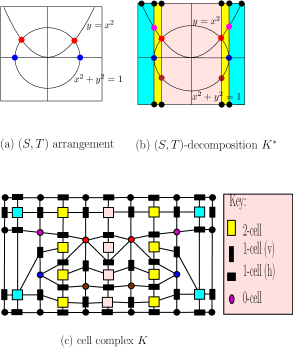
Figure 1: Arrangement of two curves, $y=x^{2}$ and $x^{2}+y^{2}=1$

Our basic problem is the following: suppose we are given an $\epsilon>0$ and a region $B_{0}\subseteq{\mathbb{R}}^{2}$, called the region-of-interest or ROI, which is usually in the shape of an axes-aligned box. We want to compute an $\epsilon$-approximation to the arrangement of the pair $(S,T)$ of curves restricted to $B_{0}$. This will be a planar straightline graph $G=(V,E)$ where $V$ is a finite set of points in $B_{0}$ and $E$ is a set of polygonal paths in $B_{0}$. Each path $e\in V$ connects a pair of points in $V$, and no path intersects another path or any point in $V$ (except at endpoints). Moreover, $E$ is partitioned into two sets $E=E_{S}\cup E_{T}$ such that $\cup E_{T}$ (resp., $\cup E_{S}$) is an approximation of $T$ (resp., $S$). The correctness of this graph $G$ has two aspects: (A) topological correctness, and (B) geometric correctness. Geometric correctness (B) is easy to formulate: it requires that the set $\cup E_{S}\subseteq B_{0}$ is $\epsilon$-close to $S$ in the sense of Hausdorff distance: $d_{H}(S,\cup E_{S})\leq\epsilon$. Similarly, the $\cup E_{T}$ is $\epsilon$-close to $T$. If we specify $\epsilon=\infty$, then we are basically unconcerned about geometric closeness.

Topological correctness (A) is harder to capture. One definition is based on the notion of “cell decomposition”. A (cell) decomposition of $B_{0}$ is a partition $K^{*}$ of $B_{0}$ into a collection of sets called cells, each $c^{*}\in K^{*}$ homeomorphic to a closed $i$-dimensional ball ($i\in\{0,1,2\}$); we call $c^{*}$ an $i$-cell and its dimension is $\dim(c^{*})=i$. If $b^{*}$ is an $i$-cell and $c^{*}$ an $(i+1)$-cell, we say $b^{*}$ bounds $c^{*}$ if $b^{*}$ is contained in the boundary $\partial c^{*}$ of $c^{*}$. Call $K^{*}$ an $(S,T)$-decomposition of $B_{0}$ if the set $(S\cup T)\cap B_{0}$ is a union of some subset of $0$- and $1$-cells of $K^{*}$. A $(S,T)$-decomposition is illustrated in Figure 1(b).

A cell complex $K$ is an (abstract) set such that each $c\in K$ has a specified $\dim(c)\in\{0,1,2\}$ together with a binary relation $B\subseteq K\times K$ such that $(b,c)\in B$ implies $\dim(b)+1=\dim(c)$. We say that the decomposition $K^{*}$ is a realization of $K$, or $K$ is an abstraction of $K^{*}$, if there is a 1-1 correspondence between the cells $c^{*}$ of $K^{*}$ with the elements $c\in K$ such that $\dim(c^{*})=\dim(c)$, and moreover the relation $(b,c)\in B$ iff $b^{*}$ bounds $c^{*}$ in $K^{*}$. Figure 1(c) shows the abstraction $K$ of the decomposition in Figure 1(b).

Our algorithmic goal is to compute a planar straightline graph (PSLG for short [19]) $G=(V,E)$ which approximates $(S,T)$ in a box $B_{0}$. Such a graph $G$ naturally determines a decomposition $K^{*}(G)$ of $B_{0}$ as follows: the set of $0$-cells is $V$, the set of $1$-cells is $E$ and the set of $2$-cells is simply the connected components of $B_{0}\setminus(V\cup(\bigcup E))$. Finally, we say $G$ is topologically correct if there exists an $(S,T)$-decomposition $K^{*}$ such that $K^{*}$ and $K^{*}(G)$ are realizations of the same abstract cell complex.

¶1. Towards Numerical Computational Geometry.

The overall agenda in this line of research is to explore new modalities for designing geometric algorithms. We are interested in exploiting weaker numerical primitives that are only complete in a certain limiting sense. Unlike traditional exact algorithms, our algorithms must strongly interact with these weaker primitives, and exploit adaptivity. The key challenge is to achieve the kind of exactness and guarantees that is typically missing in numerical algorithms. See [26] for a discussion of “numerical computational geometry”.

In the algebraic approach, one must compute the abstract complex $K$ before the approximate embedded graph $G$. Indeed, most algebraic algorithms do not fully address the computation of $G$. In contrast to such a “decoupled” approach, our algorithm provides an integrated approach whereby we can commence to compute $G$ (incrementally) even before we know $K$ in its entirety. Ultimately, we would be able to determine $K$ exactly — this can be done using zero bounds as in [25, 4]. The advantage here is that our integrated approach can cut off this computation at any desired resolution, without fully resolving all aspects of the topology. This is useful in applications like visualization.

Unlike exact algebraic primitives, our use of analytic (numerical) primitives means that our approach is applicable to the much larger class of analytic curves. Numerical algorithms are relatively easy to implement and have adaptive as well as “local” complexity. Adaptive means that the worst case complexity does not characterize the complexity for most inputs, and local means the computational effort is restricted to ROI.

One disadvantage of our current method is that it places some strong restrictions on the class of curve arrangements: the curves must be non-singular with pairwise transversal intersections in the ROI. In practice, these restrictions can be ameliorated in different ways. The complete removal of such restrictions is a topic of great research interest.

The algorithms in this paper fall under the popular literature on Marching-cube type algorithms [16]. There are many heuristic algorithms here which are widely used. The input for these algorithms can vary considerably. E.g., Varadhan et al. [24, 23] discuss input functions $F:{\mathbb{R}}^{3}\to{\mathbb{R}}$ that might be a discretized function, or a CSG model or some polygonal model – each assumption has its own exactness challenge.

2 Our Approach: Isotopic Curves Arrangement

All current exact algorithms for curve arrangements are based on algebraic projection, i.e., they need some resultant computation. The disadvantage of projection is the large number of cells: even in relatively simple examples, the graph can be large as seen as Figure 1(c). For many applications, the 2-cells may be omitted, but the graph remains large. There are several known techniques to reduce this (double-exponential in dimension) explosion in the number of cells. In this paper, we avoid cell decomposition, but base our topological correctness on the concept of isotopy. Our algorithm uses the well-known subdivision paradigm, and produces a subdivision of the input domain into boxes. Figure LABEL:fig:eg50 illustrates the form of output from our subdivision algorithm using our previous example of $y=x^{2}$ and $x^{2}+y^{2}=1$. The number of subdivision boxes tend to be even more numerous than cells in the decomposition approach. But these numbers are not directly comparable to number of cells for three reasons: (1) Subdivision boxes are very cheap to generate. (2) Most of these boxes can be instantly discarded as inessential for the final output (we keep them for visualization purposes). (3) Unlike cells, our subdivision boxes play a double role: they are used for (A) topological determination as well as (B) in determining geometric accuracy.

The approach of this paper has previously been successfully applied to the isotopic approximation of a single non-singular curve or surface by Plantinga and Vegter [18, 17] and Lin and Yap [11, 10]. The current paper is a non-trivial extension of these previous works.

We now define the notion of isotopy for arrangements. For our problem on arrangements, we need to extend the standard definitions of isotopy. Suppose $S,T\subseteq{\mathbb{R}}^{2}$ are two closed sets and $\epsilon>0$. First recall that $S$ and $T$ are (ambient) isotopic if there exists a continuous mapping

$$\gamma:[0,1]\times{\mathbb{R}}^{2}\to{\mathbb{R}}^{2}$$ (1)

such that for each $t\in[0,1]$, the function $\gamma_{t}:{\mathbb{R}}^{2}\to{\mathbb{R}}^{2}$ (with $\gamma_{t}(x,y)=\gamma(t,x,y)$) is a homeomorphism, $\gamma_{0}$ is the identity map, and $\gamma_{1}(S)=T$. If, in addition, $d_{H}(S,T)\leq\epsilon$ (where $d_{H}$ is the Hausdorff distance on closed sets) we say that they are $\epsilon$-isotopic. We will write

$$S\stackrel{{\scriptstyle\epsilon}}{{\simeq}}T~{}(\mathrm{via}~{}\gamma)$$

in this case. Note that we may omit mention of $\epsilon$, in which case it is assumed that $\epsilon=\infty$.

We now generalize this to arrangement of sets. Let $\overline{S}=(S_{1},\ldots,S_{m})$ and $\overline{T}=(T_{1},\ldots,T_{m})$ be two sequences of $m$ closed sets. For each non-empty subset $J\subseteq\{1,2,\ldots,m\}$, let $\overline{S}_{J}$ denote the intersection $\cap_{i\in J}S_{i}$. Similarly for $\overline{T}_{J}$. We say that $\overline{S}$ and $\overline{T}$ are isotopic if there exists a continuous mapping $\gamma$ as in (1) such that for each non-empty subset $J\subseteq\{1,2,\ldots,m\}$, we have

$$\overline{S}_{J}\stackrel{{\scriptstyle\epsilon}}{{\simeq}}\overline{T}_{J}~{}(\mathrm{via}~{}\gamma).$$

We also call $\gamma$ an isotopy from $\overline{S}$ to $\overline{T}$. For simple curve arrangements, the critical problem to solve is the case $m=2$. We assume the two curves $S_{1},S_{2}$ are restricted to a region or box $B$. Our basic problem is to compute a pair of curves $(T_{1},T_{2})$ such that

$$(T_{1},T_{2})\stackrel{{\scriptstyle\epsilon}}{{\simeq}}(S_{1}\cap B,S_{2}\cap B).$$ (2)

The approximations $(T_{1},T_{2})$ produced by our algorithms will be piecewise linear curves. See [1] for a general discussion of isotopy of the case $m=1$.

2.1 Normalization relative to a Subdivision Tree

In Appendix A, we provide the necessary definitions; these are consistent with the terminology in the related work [11]. For now, we rely on common terms that are mostly self-explanatory.

¶2. Box Complexes and Subdivision Trees.

Our fundamental data structure is a subdivision tree ${\cal T}$ rooted in some box $B_{0}$. In 2-D, ${\cal T}$ is the well-known quad-tree and $B_{0}$ is a rectangle. Each internal node of ${\cal T}$ has four congruent children. The boxes of a subdivision tree are non-degenerate (i.e., $2$-dimensional). They need not be squares, but for the correctness of our algorithm, their aspect ratios must be $\leq 2$. For any region $R\subseteq{\mathbb{R}}^{2}$, we define a subdivision of $R$ to be a set $\SS=\{R_{1},\ldots,R_{n}\}$ of subregions such that $R=\cup_{i=1}^{n}R_{i}$ and the interiors of $R_{i}$’s are pairwise disjoint. If each $R_{i}$ is a box, we call $\SS$ a box subdivision. The box subdivision is a box complex if for any two adjacent boxes $B,B^{\prime}\in\SS$, their intersection $\partial(B)\cap\partial(B^{\prime})$ is side of either $B$ or $B^{\prime}$. Clearly, the set $\SS$ of leaf boxes of ${\cal T}$ forms a box complex of $B_{0}$. But in this paper, we need to consider a more general subdivision of $B_{0}$ that is obtained as the leaf boxes of a finite number of subdivision trees. A segment of a box complex $\SS$ is the side of a box of $\SS$ that does not properly contain the side of an adjacent box. Therefore every side of a box of $\SS$ is a finite union of segments. We say the box complex $\SS$ is balanced if every side is either a segment or the union of two segments. A segment is called bichromatic w.r.t. a curve $S$ if $S$ has different signs on the endpoints of the segment; otherwise call it monochromatic.

Although $(S,T)$ is simple, we need to consider degeneracies induced by a subdivision $\SS$: we say $(S,T)$ is $\SS$-regular if $S\cup T$ does not intersect any corner of a box in $\SS$. This can be effectively achieved by an infinitesimal perturbation of $S$ and $T$ using a trick in [18]: when we evaluate the sign of $f$ at a box corner, we simply regard a $0$ sign to be $+1$.

¶3. Normalization.

Consider an isotopy of the arrangement $(S,T)$ into another arrangement $(S^{\prime},T^{\prime})$. Let us write $(S,T)_{t}$ for the arrangement at time $t\in[0,1]$ during this transformation. Thus $(S,T)_{0}=(S,T)$ and $(S,T)_{1}=(S^{\prime},T^{\prime})$. The isotopy is said to $\SS$-regular provided, for all $t\in[0,1]$, $(S,T)_{t}$ is $\SS$-regular. We say that $(S,T)$ is $\SS$-normalized if:

• $(S,T)$ is $\SS$-regular.

• Each subdivision box $B$ of $\SS$ contains at most one point of $S\cap T$.

• Let $X\in\{S,T\}$. Then $X$ intersects each segment of $\SS$ at most once

Call $(S^{\prime},T^{\prime})$ a $\SS$-normalization of $(S,T)$ if there exists a $\SS$-regular isotopy from $(S,T)$ to $(S^{\prime},T^{\prime})$ such that $(S^{\prime},T^{\prime})$ is $\SS$-normalized. Our algorithm will construct an $\SS$-normalization $(S^{\prime},T^{\prime})$ of $(S,T)$.

¶4. Box Predicates.

We will use a variety of box predicates. These predicates will determine the subdivision process. Typically, we will keep subdividing boxes until some Boolean combination of some box predicates hold.

Let $h:{\mathbb{R}}^{2}\to{\mathbb{R}}$ be any real function. Recall (Appendix A) that we assume an interval formulation of $h$ denoted ${\framebox(4.0,7.0)[]{}\,}h:{\framebox(4.0,7.0)[]{}\,}{\mathbb{R}}^{2}\to{\framebox(4.0,7.0)[]{}\,}{\mathbb{R}}$ where ${\framebox(4.0,7.0)[]{}\,}{\mathbb{R}}$ denotes the set of closed intervals and ${\framebox(4.0,7.0)[]{}\,}{\mathbb{R}}^{2}$ can be viewed as the set of boxes. We introduce a pair of box predicates denoted $C_{0}^{h}$ and $C_{1}^{h}$, defined as

$$\left.\begin{array}[]{lllllllllllllllllllllllll}C_{0}^{h}(B)&\equiv&0\not\in{\framebox(4.0,7.0)[]{}\,}h(B),\\ C_{1}^{h}(B)&\equiv&0\not\in({\framebox(4.0,7.0)[]{}\,}h_{x}(B))^{2}+({\framebox(4.0,7.0)[]{}\,}h_{y}(B))^{2}.\end{array}\right\}$$ (3)

Note that $C_{1}^{h}$ as taken from Plantinga-Vegter, where the interval operation $I^{2}$ is defined as $\{xy:x,y\in I\}$ and not $\{x^{2}:x\in I\}$. An alternative to $C_{1}^{h}$ would be the weaker $C_{xy}^{h}$ predicate from Lin-Yap [11], but the corresponding algorithm would would be more involved. So for now, we focus on the $C_{1}^{h}$ predicate. We classify boxes using these predicates:

• Box $B$ is $h$-excluded if it satisfies $C_{0}^{h}(B)$.

• Box $B$ is $h$-included if it fails $C_{0}^{h}(B)$ but satisfies $C_{1}^{h}(B)$.

• Box $B$ is resolved if it satisfies the predicate

  $$(C_{0}^{f}\lor C_{1}^{f})\land(C_{0}^{g}\lor C_{1}^{g}).$$ (4)

• Box $B$ is excluded if it satisfies $C_{0}^{f}\land C_{0}^{g}$. Note that excluded boxes are resolved.

• Box $B$ is a candidate if it is resolved but not excluded.

• Candidate boxes can be further classified into three subtypes: $f$-candidates are those that are $f$-included but $g$-excluded, $g$-candidates is similarly defined, and $fg$-candidates are those that are $f$- and $g$-included.

¶5. Root Boxes.

We define a root box to be any box $B$ where $B\cap S\cap T$ has exactly one point. We next consider two predicates that will allow us to detect root boxes. One is the Jacobian condition,

$$\mathrm{JC}(B)\equiv 0\notin\det({\framebox(4.0,7.0)[]{}\,}J_{F}(B))$$

where ${\framebox(4.0,7.0)[]{}\,}J_{F}(B)$ is the Jacobian of $F=(f,g)$ evaluated on $B$. If $\mathrm{JC}(B)$ holds, then $B$ has at most one root of $f=g=0$, The other is the Moore-Kioustelidis condition $\mathrm{MK}(B)$ [14] which can be viewed as a preconditioned form of the famous Miranda Test [8]; for other existence tests based on interval arithmetic see [6]. If $\mathrm{MK}(B)$ holds, then $B$ has at least one root of $f=g=0$. We provide the details for this predicate in Appendix B; see (9). Therefore, when $\mathrm{JC}(B)$ and $\mathrm{MK}(B)$ holds, we know that $B$ is a root box. The use of Miranda’s test combined with the Jacobian condition has been used earlier to isolate the common roots [12]. What is new in this paper is its application to the simple curve arrangement problem.

2.2 Graph Representation

Our algorithm will produce a graph $G=(V,E)$ where vertices $v\in V$ are points in ${\mathbb{R}}^{2}$ and edges are line segments connecting pairs of vertices. Moreover, each edge $E$ will be labeled as an $S$-edge or a $T$-edge. The union of these edges will provide a polygonal $\epsilon$-approximation of $(S,T)$. We now give an overview of the issues and solution.

First, we describe how the vertices of $V$ are introduced.

• We introduce a vertex in the center of a root box $B$.

• We evaluate $f,g$ at the endpoints of segments of $B$. If $h\in\{f,g\}$ is bichromatic on a segment of $B$, then we must introduce an $h$-vertex somewhere in the segment. In a balanced subdivision, an $\SS$-normalized pair $(S^{\prime},T^{\prime})$ of curves has at most two $h$-vertices on an edge of a box $B$.

• Introducing vertices on the edges of a box $B$ is straightforward if $B$ is an $f$-candidate or a $g$-candidate. When $B$ is a $fg$-candidate, we may have an edge $e$ containing both a $f$-vertex and a $g$-vertex. In the next section we will show how to find the relative order of these two vertices.

Next we discuss how to introduce the edges $E$, which are line segments completely contained in a box.

• If $B$ is a root box, we just connect the vertex at its midpoint $\mathrm{cen}(B)$ to each of the vertices on the edges of $B$. There will be exactly two $f$-vertices and two $g$-vertices.

• If $B$ is a $f$-candidate or $g$-candidate, then the connection is trivial in the regular case. In the balanced case, the rules from the previous work of Plantinga-Vegter [18] assures us of the correct connection.

• If $B$ is a $fg$-candidate, but not a root box, we know that the $f$-segment and $g$-segment will not intersect. Some $fg$-candidates need global information to resolve them: when there are two edges where each edge contains both an $f$- and a $g$-vertex. Their relative order must be determined globally from root boxes or from boxes where their relative order is known. We will show how to propagate this information in §3.

2.3 Curve Arrangement in Root Boxes

Suppose $(S^{\prime},T^{\prime})$ is the normalization of $(S,T)$ relative to the box $B$, i.e., $(S^{\prime},T^{\prime})$ is an isotopic transformation of $(S,T)$ which respects the four corners of $B$. We now determine the isotopy type of $(S^{\prime},T^{\prime})$ in a root box $B$. The possible combinatorial types fall under one of the $8$ patterns as shown in Figure 2. We put them in three groups (I, II, III) for our analysis.

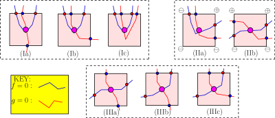
Figure 2: Local intersection patterns of the normalized curves $(S^{\prime},T^{\prime})$

Following the standard Marching Cube technique, we evaluate the sign of the functions $f,g$ at the four corners of $B$. If $f$ has different signs at the endpoints of an edge $e$ of $B$, then we must introduce an $f$-vertex somewhere in the interior of $e$. Our normalization assumptions imply that there are either zero or two $f$-vertices on the boundary of $B$. We treat $g$ similarly. Our aim is to connect the two $f$-vertices, the two $g$-vertices, and a point in the center of the box which represents the common root with line segments such that the graph $G$ obtained is an isotopic approximation of $(S^{\prime}\cap B_{0},T^{\prime}\cap B_{0})$. There is a subtlety: the method exploits “local non-isotopy” [18, 11], meaning that we do not guarantee that $S\cap B$ is isotopic to the segment introduced to connect two $f$-vertices. However, the graph $G$ will be locally isotopic to the normalized curves $(S^{\prime},T^{\prime})$, i.e., $G\cap B$ is isotopic to $(S^{\prime}\cap B,T^{\prime}\cap B)$ in each subdivision box $B$.

The issue before us is the relative placements of an $f$-vertex and $g$-vertex in case they both occur in $e$; e.g., the patterns in group II in Figure 2. The main result of this section is the following.

Theorem 1.

Let $B$ be a root box that satisfies $\mathrm{MK}(B)$. Then the signs of $f$ and $g$ at each of the four corners of $B$ determine the combinatorial type of the normalized curves $S^{\prime},T^{\prime}$ in $B$. Moreover, these combinatorial types fall under one of the five types in Groups II and III in Figure 2.

The main idea of the proof is that if $\mathrm{MK}(B)$ holds for a box $B$ then there exists an edge $e$ of $B$ such that either $f(e)>cg(e)$, or $g(e)>cf(e)$, for some $c>0$. Given such an $e$, we can find the relative order of the $f$-vertex and $g$-vertex on $e$. See Appendix C for details of the proof.

2.4 Geometry of Extended Root Boxes

By an aligned box we mean one that can be obtained as a node of a subdivision tree rooted at the region-of-interest (ROI) $B_{0}$; otherwise, it is said to be non-aligned. For instance, in Figure 3(a), let the box with corners $p,q,r,s$ be $B_{0}$. Then the figure shows the four children of $B_{0}$, which are aligned, as well as the non-aligned box $(1/2)B_{0}$ whose corners are $p^{\prime},q^{\prime},r^{\prime},s^{\prime}$. Note that $(1/2)B_{0}$ can be obtained as the union of aligned boxes. We are interested in non-aligned boxes that can be obtained as a finite union of aligned boxes. In the simplest case of non-alignment, a box $B$ is said to be half-aligned if it is equal to the union of congruent aligned boxes of size $w(B)/2$. Thus if $B$ is aligned then both $(1/2)B$ and $2B$ are half-aligned.

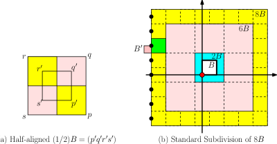
Figure 3: (a) $B=(pqrs)$ is aligned, (b) $2B$ is a root box.

In most subdivision algorithms, it is enough to work with aligned boxes. But to treat root boxes, we see an essential need to work with non-aligned boxes. The reason is that if we apply the Moore-Kioustelidis predicate to aligned boxes, non-termination may occur when a root of $F$ lies on the boundary of an aligned boxes. But such roots can be detected in the interior of non-aligned boxes. This issue is often ignored in the literature, but it needs to be properly treated in exact algorithms. Some discussions may be found in Stahl [22] and Kamath [7]; in the univariate case, a solution is suggested by Rote [20] for splines.

Therefore, given an aligned box $B$, we provide a procedure to detect if $2B$ is a root box. We consider the nested sequence of boxes $B\subset 2B\subset 6B\subset 8B$ as illustrated in figure 3(b). Our goal is to detect $2B$ as a root box, but because of alignment issues, we must also treat the larger box $8B$ which is called the extended root box corresponding to $B$.

We construct the following standard subdivision of $8B$, denoted $\mathrm{Std}(B)$, into sub-boxes:

• Subdivide $6B$ into $9$ boxes, each congruent to $2B$ (indeed, $2B$ is one of these $9$ boxes).

• The annular region $8B\setminus 6B$ is partitioned into $28$ boxes, each congruent to $B$. These are called the ring boxes.

See Figure 3(b) for illustration. Note that $\mathrm{Std}(B)$ is balanced. None of the subdivision boxes are aligned, but the ring boxes are half-aligned.

¶6. Conforming Subdivisions.

Let $\Pi$ be a subdivision of a region $R$. A box $B^{\prime}\in\Pi$ is a boundary box of the subdivision if $\partial B^{\prime}$ intersects $\partial R$. In the following definitions, we fix a region $R_{0}\subseteq B_{0}$ and fix a box $B$ such that $8B\subseteq R_{0}$. Also let $k\geq 1$ be an integer.

A subdivision $\Pi_{0}$ for $R_{0}\setminus 8B$ is called externally $k$-conforming for $B$ if it has three properties: $\Pi_{0}$ is balanced, the union $\Pi_{0}\cup\{8B\}$ is a box complex, and for each box $B^{\prime}\in\Pi_{0}$, if $B^{\prime}$ is adjacent to $8B$ then $w(B^{\prime})=w(B)/2^{k}$. A subdivision $\Pi_{1}$ of $8B$ is called internally $k$-conforming for $B$ if $\Pi_{1}$ is balanced, and for every boundary box $B^{\prime}$ of $\Pi_{1}$, $w(B^{\prime})=w(B)/2^{k-1}$. Note for instance that if $\Pi_{1}$ is the standard subdivision of $8B$, then it is internally $1$-conforming for $B$. Below we show how to achieve subdivisions of $8B$ that is internally $k$-conforming for $B$ for $k\geq 2$. The following is immediate: If $\Pi_{0}$ is externally $k$-conforming for $B$, and $\Pi_{1}$ is internally $k$-conforming for $B$, then their union $\Pi_{0}\cup\Pi_{1}$ is a balanced subdivision of $R_{0}$. Note that if $k>1$ then getting a balanced subdivision of $\Pi_{0}\cup\Pi_{1}$ may cause the edges of a root box $2B$ to split into two segments (but not more); see Figure 4. This can be handled by a case analysis similar to Theorem 1 based on Lemma 7. An alternative approach is to replace $8B$ by $10B$ which would have an extra ring of boxes congruent to $B$. In this case, we can handle any $k>1$ by subdividing this outermost ring, but without affecting the standard subdivision of $8B$. This gives a simple and effective solution.

¶7. Strong Root Isolation.

Suppose $2B$ is a root box. We say $2B$ is strongly isolated if the following conditions hold

• (P1) The following four predicates hold: $C_{1}^{f}(8B),C_{1}^{g}(8B),\mathrm{JC}(6B),\mathrm{MK}(2B)$.

• (P2) $F=(f,g)$ has no roots in the annulus $8B\setminus 2B$.

The predicates in (P1) ensures that $2B$ is a root box. It is not hard to see that if $2B$ contains a root of $F$ and is sufficiently small, then properties (P1) and (P2) will hold. The reason for $\mathrm{MK}(2B)$ (not just $\mathrm{MK}(B)$ is to ensure that we test the Moore-Kioustelidis predicate on overlapping boxes, so that roots on the boundary of an aligned box $B$ will appear in the interior of $2B$. The reason for $\mathrm{JC}(6B)$ instead of $\mathrm{JC}(2B)$ is that there can be two boxes $2B$ and $2B^{\prime}$ such that both of them satisfy MK-test and they overlap. The test $\mathrm{JC}(6B)$ ensures that if there are two such boxes then they correspond to the same root, and so discard one of them.

¶8. Root Refinement:

Let $B$ be an aligned box from the subdivision queue such that $2B$ is a root box. We give a subroutine to refine such a root box $2B$. It it important that in our refinement method all the sub-boxes remain dyadic boxes, assuming the input boxes are dyadic. The idea is to cover $2B$ with a covering of aligned boxes, which must be of size $w(B)/2$, and check whether MK-test holds for the doubling of any of these 16 boxes. If not, then subdivide these boxes and continue recursively with the $fg$-candidates. See Appendix A for more details.

3 Algorithm for Curve Arrangement

Our overall algorithm begins with the (trivial) subdivision tree ${\cal T}$ rooted at the ROI $B_{0}$ but with no other nodes. The algorithm amounts to repeatedly expansion of the candidate leafs in ${\cal T}$ until a variety of global properties hold. We given an overview of the algorithm in a sequence of 9 stages; see Appendix C.

¶9. Stage I: Resolution Subdivision

The high level description of this stage is easy: keep expanding any leaf $B$ of ${\cal T}$ that is not resolved (see (4)). Recall that resolved boxes are either excluded or candidates. As each box is resolved, it is placed in one of the following four queues: $Q_{0}$ for excluded boxes, $Q_{f}$ for $f$-candidates, $Q_{g}$ for $g$-candidates, and $Q_{fg}$ for $fg$-candidates Besides these four global queues, we also use these additional queues: $Q_{\mathrm{JC}},Q_{\mathrm{MK}},Q_{\mathrm{Root}}$ corresponding roughly to boxes that satisfies the $\mathrm{JC}$ and $\mathrm{MK}$ predicates, or are found to be root boxes. The boxes in all the queues are always aligned boxes.

¶10. Stage II: Jacobian Stage.

Remove a box $B$ from $Q_{fg}$ and do the following: If $\mathrm{JC}(6B)$ holds then put $B$ into $Q_{\mathrm{JC}}$, otherwise, subdivide $B$ and distribute the children into $Q_{0},Q_{f},Q_{g},Q_{fg}$.

¶11. Stage III: MK Stage.

For every box $B\in Q_{\mathrm{JC}}$ we subdivide it until either we find a sub-box $B^{\prime}$ such that $\mathrm{MK}(2B^{\prime})$ holds, or we have identified all sub-boxes as one of $Q_{0},Q_{f},Q_{g},Q_{fg}$.

¶12. Stage IV: Strong Root Isolation Stage

We assume that $Q_{\mathrm{MK}}$ is a priority queue, where boxes are popped starting from the largest size. For each such box $B$ check whether $8B$ is disjoint from $8B^{\prime}$, for all its neighbors $B^{\prime}$; if not then replace $B$ with RefineRoot$(B)$. We now have obtained a queue $Q_{\mathrm{Root}}$ containing root boxes for all the roots in ROI. The next step is to externally conform $\mathrm{Std}(B)$ with the rest of the subdivision tree ${\cal T}$.

¶13. Stage V: Pruning ${\cal T}$

In this stage we will turn OFF some leaf boxes in $On({\cal T})$ depending on how they interact with the extended root boxes $8B$. The aim is to “blackout” the $8B$ regions from ROI, and ensure that the boxes abutting it are all aligned boxes. Let $B^{\prime}$ be the great-grandparent of $B$ in ${\cal T}$. Then we get the list of leaf boxes that cover the interior of $B^{\prime}$ and another list of boxes that are its neighbors. For each box $B_{\mathrm{tmp}}$ in these lists, we turn it OFF if it is contained in $8B$; if it overlaps $8B$ then we subdivided it and proceed with its children. Let ${\cal T}^{\prime}$ be the resulting subdivision tree.

¶14. Stage VI: Balancing and Externally Conforming

Recall the standard balancing procedure for a subdivision ${\cal T}$ of a region $B_{0}$ from the appendix. We will construct a balanced and externally conformal subdivision of $B_{0}\setminus\cup_{i}8B_{i}$, where $8B_{i}$’s are pairwise disjoint extended root boxes. For each box $8B_{i}$, we add a conceptual box to ${\cal T}^{\prime}$, with depth either one more than its smallest neighbor, or if all the neighbors of $8B$ are larger than $w(B)$ then one more than the depth of $B$ in ${\cal T}$. Call the standard balancing procedure on the modified ${\cal T}^{\prime}$. By Lemma 3, we will get the desired subdivision; after balancing the boxes bordering $8B$ will all be of the same size, namely $w(B)/2^{k}$, for some $k\geq 1$.

¶15. Stage VII: Internally Conforming Extended Root Boxes

Consider any extended root box $8B$ and its standard subdivision $\mathrm{Std}(B)$. Given a $k>1$ from the previous stage, we want to balance the interior and the exterior of $\mathrm{Std}(B)$. Note that since $k>1$ the boxes on the exterior are always smaller than all the boxes in $\mathrm{Std}(B)$. To get a balanced conformal subdivision of $\mathrm{Std}(B)$, we initialize a priority queue $Q$ with all the boxes on the exterior of $8B$ (all of them are of the same size) and the 37 boxes in $\mathrm{Std}(B)$. Then we initiate the standard balancing procedure on $Q$. See Figure 4(c) for an illustration of this procedure; the box $B^{\prime}$ has width $w(B)/8$. We do this balancing step for each of the extended root boxes $8B$. The union of these subdivisions with the balanced subdivision of $B_{0}\setminus\cup_{i}8B_{i}$ gives us a balanced subdivision of $B_{0}$, our ROI.

¶16. Stage VIII: PV-Construction

For each box in $Q_{f}$, connect its two $f$-vertices with a line segment; do the same for boxes in $Q_{g}$. For each box in $Q_{\mathrm{Root}}$ place a vertex at its center and connect the two $f$-vertices and the two $g$-vertices with this vertex according to the cases shown in Groups II and III. of Figure 2. At the end of this stage, the only queue that remains unprocessed is $Q_{fg}$. The next stage resolves these boxes.

¶17. Stage IX: Resolving Ambiguous $fg$-candidates

We call an $fg$-candidate box ambiguous if they have the same set of bichromatic segments; otherwise, call the box unambiguous. By definition, boxes where $f$ and $g$ do not share a bichromatic segment are unambiguous. However, some ambiguous boxes can be made unambiguous locally. From Theorem 1 we know that ambiguous root boxes can be made unambiguous. Also, boxes where the two shared bichromatic segments are on adjacent edges can be made unambiguous by repeated subdivisions of the edges until we reach a segment in one of the edges that is bichromatic for one curve and monochromatic for the other; this will happen along one of the edges since both $C_{1}^{f}$ and $C_{1}^{g}$ hold. A similar approach works to resolve ambiguous boxes that share an edge with $B_{0}$ and a common bichromatic segment is on this edge, because by assumption boundary of $B_{0}$ does not contain a root of $f,g$. From these unambiguous boxes, we propagate the ordering of the $f$-vertex and $g$-vertex on the shared edge to their ambiguous neighbors.

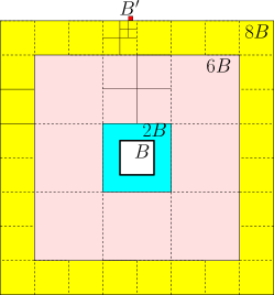
Figure 4: An internally conformal subdivision of $\mathrm{Std}(B)$.

¶18. Correctness of Algorithm

We must prove that our graph $G=(V,E)$ is isotopic to the arrangement $(S,T)$ in box $B_{0}$. Suppose there are $k$ roots, $|S\cap T|=k$. Our correctness requires that none of these roots lie in $\partial B_{0}$. Our algorithm produces the following data: we have “well isolated” the roots in this sense: we have found $k$ aligned boxes, $B_{1},\ldots,B_{k}$ such that $2B_{i}$ is a root box, $8B_{i}\subseteq B_{0}$, and the interiors of the $8B_{i}$’s are pairwise disjoint. Next, we have constructed subdivisions,

$$\SS_{0},\SS_{1},\ldots,\SS_{k}$$

where $\SS_{i}$ is a subdivision of $8B_{i}$ ($i=1,\ldots,k$) and $\SS_{0}$ is a subdivision of $B_{0}\setminus\cup_{i=1}^{k}8B_{i}$. Moreover, the union of all these subdivisions, denoted $\SS^{*}$, constitutes a balanced box complex of $B_{0}$.

Theorem 2.

The PSLG $G$ computed by the algorithm is a $\SS^{*}$-normalization of the curves $(S,T)$.

We sketch the arguments here: let $(S^{\prime},T^{\prime})$ be a $\SS^{*}$-normalization of $(S,T)$. The graph $G$ will be obtained as the union of $G_{B}$ for all $B\in\SS^{*}$, where each $G_{B}$ is a PSLG contained in box $B$. We know from Theorem 1 how to construct a PSLG $G_{B}\subseteq B$ that is isotopic to $(S^{\prime},T^{\prime})$ in each root box $B$. We know from Plantinga-Vegter how to construct PSLG $G_{B}^{S}$ that are isotopic to $S^{\prime}$ in each non-root box $B$. Similarly we have $G_{B}^{T}$. But we need to form their ”union”, which is the PSLG $G_{B}$ that is isotopic to $(S^{\prime},T^{\prime})$ in $B$. For this purpose, we need to know the relative ordering of the $f$-vertex and $g$-vertex on each segment of $B$ that is bichromatic for both curves. This information is resolved by Stage IX of our construction.

4 Final Remarks

We have presented a complete numerical algorithm for the isotopic arrangement of two simple curves. The underlying paradigm is Domain Subdivision, coupled with box predicates and effective forms of the Miranda Test. Moreover, we crucially exploit the previous isotopic approximation algorithms of Plantinga-Vegter [18] for a single curve.

The algorithm is very implementable: despite the many stages, each stage involves iteration using well-known data structures. A full implementation and comparisons with other methods is planned; we have currently implemented the root isolation part.

The extension of this work to the simple arrangement of multiple curves is of great interest. Many of the techniques we have developed for 2 curves will obviously extend. One possible way to use our work for multiple curves is as follows: first compute the root boxes $2B_{i}$ of all the pairwise intersections, and make them “well isolated” in the sense that $8B_{i}$ boxes are pairwise disjoint, as before. Then we compute a balanced, conforming subdivision $\SS_{0}$ of complement of the union of these $8B$ boxes. Moreover, we need to resolve ambiguities, i.e., relative ordering of curves on a common segment. Some of this can be resolved by propagation, but there will be need for recursive subdivision in general. In the full paper, we will provide such a description.

A general open problem is to prove polynomial complexity bounds for such subdivision algorithms. As a first step, we would like to prove that the root isolation part is polynomial-time. This would be a generalization of our recent work on continuous amortization for real and complex roots [21].

Appendix A Basic Concepts

We fix the terminology for well-known concepts in boxes, interval arithmetic and subdivision trees. We define these concepts in $d$-dimensions. Of course, the algorithms in this paper work in $d=2$.

¶19. Boxes.

Let ${\framebox(4.0,7.0)[]{}\,}{\mathbb{R}}$ denote the set of closed intervals. We may identify ${\mathbb{R}}$ with degenerate intervals $[a,a]\in{\framebox(4.0,7.0)[]{}\,}{\mathbb{R}}$. Also ${\framebox(4.0,7.0)[]{}\,}{\mathbb{R}}^{d}$ is the $d$-fold Cartesian product of ${\framebox(4.0,7.0)[]{}\,}{\mathbb{R}}$. Elements of ${\framebox(4.0,7.0)[]{}\,}{\mathbb{R}}^{d}$ are called $d$-boxes. The width of $B$ is $(w(I_{1}),\ldots,w(I_{d}))$ where the width of an interval $I=[a,b]$ is $w(I)=b-a$. the same (resp., differ by at most $1$). If $B,B^{\prime}$ are two boxes in ${\framebox(4.0,7.0)[]{}\,}{\mathbb{R}}^{d}$, we say they are $k$-neighbors if $B\cap B^{\prime}$ has dimension $k$. So $k\in\{-1,0,1,d-1\}$, where the empty set has dimension $-1$. We say $B$ and $B^{\prime}$ are adjacent if they are $(d-1)$-neighbors. Each box has $2^{d}$ sides (sometimes called edges) and $2^{d}$ corners. The boundary of a box $B$ is denoted $\partial B$.

¶20. Box Functions.

Interval arithmetic [13] is central to our computational toolkit. If $f:{\mathbb{R}}^{d}\to{\mathbb{R}}$ is a real function, then we call a function of the form ${\framebox(4.0,7.0)[]{}\,}f:{\framebox(4.0,7.0)[]{}\,}{\mathbb{R}}^{d}\to{\framebox(4.0,7.0)[]{}\,}{\mathbb{R}}$ an inclusion function for $f$ if for all $B\in{\framebox(4.0,7.0)[]{}\,}{\mathbb{R}}^{d}$, ${\framebox(4.0,7.0)[]{}\,}f(B)$ contains $f(B)=\{f(p):p\in B\}$. Call ${\framebox(4.0,7.0)[]{}\,}f$ a box function for $f$ if it is an inclusion function for $f$ and for all $\{B_{i}\in{\framebox(4.0,7.0)[]{}\,}{\mathbb{R}}^{d}:i\in{\mathbb{N}}\}$, if $B_{i}$ converges monotonically to a point $p\in{\mathbb{R}}$ then ${\framebox(4.0,7.0)[]{}\,}f(B_{i})$ converges monotonically to $f(p)$. Note that box functions are easy to construct for polynomials and common real functions.

¶21. Subdivision Trees.

Our fundamental data structure is a quad-tree or subdivision tree ${\cal T}$: the nodes of ${\cal T}$ are boxes in ${\framebox(4.0,7.0)[]{}\,}{\mathbb{R}}^{d}$, and each internal node $B$ has $2^{d}$ children which are congruent sub-boxes, with pairwise disjoint interiors, and whose union is $B$. In order to use ${\cal T}$ to represent regions of complex geometry, we assume that each leaf of $T$ is (arbitrarily) either turned ON or turned OFF. The union of all the ON-leaves is denoted $R({\cal T})$, called the region-of-interest (ROI). Let $On({\cal T})$ denote the set of ON-leaves of ${\cal T}$. We call $On({\cal T})$ a subdivision of $R({\cal T})$. In general, a subdivision of a set $X\subseteq{\mathbb{R}}^{d}$ is a collection $C$ of sets in ${\mathbb{R}}^{d}$ such that $\cup C=X$ and the relative interior of the sets in $C$ are pairwise disjoint. One of the basic operations on subdivision trees is to take an ON-leaf $B$ of ${\cal T}$ and to “expand it”, i.e., to split $B$ into $2^{d}$ congruent sub-boxes and attach them as children of $B$. Thus $B$ becomes an internal node and its children become leaves of the expanded ${\cal T}$. By definition, the children of $B$ remain ON-leaves. Thus the ROI is not affected by expansion.

A segment of ${\cal T}$ is a line segment of the form $B\cap B^{\prime}$ where $B,B^{\prime}$ are adjacent boxes in ${\cal T}$. Note that a segment is always an edge of some box, but some box edges are not segments. In general, an edge is subdivided into a finite number of segments.

The boxes of a subdivision tree are assumed to be non-degenerate, i.e., they are $d$-dimensional. In our algorithms, certain ON-leaves are called “candidates box”. Unless otherwise noted, we could assume every ON-leaf is a candidate box. We then say ${\cal T}$ is balanced if, for any two candidate boxes, if they are adjacent then their depths differ by at most one.

Traversing neighbors in a subdivision of ROI: Given a subdivision tree ${\cal T}$ partitioning the ROI, a crucial sub-procedure required by the algorithm is the ability to get the neighbors of a leaf-box in ${\cal T}$. One way to achieve this is to associate two pointers with every edge of a leaf box of ${\cal T}$, namely the pointers that point to the extreme neighbors along the edge (there may be only one such neighbor, in which the two pointers point to the same box). Thus we associate 8 pointers with every leaf-box. We will often say the “eight neighbors” of a box to refer to the boxes pointed by these eight pointers, where we count the boxes with multiplicity. We can list all the neighbors of a leaf-box $B$ in ${\cal T}$ using these eight pointers.

Standard Balancing Procedure:

Let $Q_{\mathrm{tmp}}$ be a priority queue of all the leaves in ${\cal T}$; the deeper the level the higher the priority. While $Q_{\mathrm{tmp}}$ is non-empty do $B\leftarrow Q_{\mathrm{tmp}}.pop()$. For each neighbor $B_{\mathrm{tmp}}$ of $B$ do If $B_{\mathrm{tmp}}$ is not balanced w.r.t. $B$ subdivide $B_{\mathrm{tmp}}$ and add its children to $Q_{\mathrm{tmp}}$.

There can be at most two neighbors of $B$ that need to be subdivided, because $B$ shares two edges with its siblings and so the boxes neighboring $B$ along those edges are balanced w.r.t. $B$; the unbalanced boxes can occur on the remaining two edges. Moreover, for any neighbor $B_{\mathrm{tmp}}$ that is subdivided only one of its children neighbors $B$. Balancing also has the following nice property, which intuitively says that the boxes produced in the ensuing subdivision cannot all be very small.

Lemma 3.

Suppose we are balancing a box $B$, and let $B^{\prime}$ be its violating larger neighbor. Let $e$ be the edge of $B^{\prime}$ shared with $B$ and $e^{\prime}$ be the opposite edge. Then the subdivision of $B^{\prime}$ caused by $B$ while balancing will split the edge $e^{\prime}$ only once.

In the subdivision tree of $B^{\prime}$, the two children that share $e^{\prime}$ are in a different subdivision tree compared to the child of $B^{\prime}$ that is adjacent to $B$ and shares $e$; see Figure 5. Balancing produces a subdivision tree of $B^{\prime}$ that has only one path, with leaves hanging from it, that ends in a box whose size is double the size of $B$. The number of leaves in this tree are $3\cdot(\log w(B^{\prime})-\log w(B)-1)$.

Figure 5: A subdivision caused balancing.

Appendix B The Moore-Kioustelidis Test for Roots

Although our paper is focused on arrangement of curves, we shall temporarily consider a more general setting of a continuous function $F:{\mathbb{R}}^{n}\to{\mathbb{R}}^{n}$ in $n$-space. Let the coordinate functions of $F$ be denoted $(f_{1},\ldots,f_{n})$. If $B=\prod_{i=1}^{n}I_{i}\subseteq{\mathbb{R}}^{n}$ is a box, we write $B_{i}^{+}$ and $B_{i}^{-}$ for the pair of faces of $B$ whose outward normal are (respectively) the positive and negative $i$th semi-axis. Thus, if $I_{i}=[a_{i},b_{i}]$ then $B_{i}^{-}=I_{1}\times\cdots\times I_{i-1}\times a_{i}\times I_{i+1}\times\cdots\times I_{n}$, and $B_{i}^{+}$ is similar, but with $b_{i}$ in place of $a_{i}$. The center of a box $B$, $\mathrm{cen}(B)$, is defined as the vector $((a_{1}+b_{1})/2,,\ldots,(a_{n}+b_{n})/2)$. For a positive real number $\lambda$, define the scaled box

$$\lambda B\mathop{\mbox{\rm:=}}\{\lambda({\bf x}-\mathrm{cen}(B)+\mathrm{cen}(B))|{\bf x}\in B\}.$$

For ${\bf X}\in{\framebox(4.0,7.0)[]{}\,}{\mathbb{R}}$, define the magnitude of ${\bf X}$, $\mathrm{mag}({\bf X})\mathop{\mbox{\rm:=}}\max_{x\in{\bf X}}\left\lvert x\right\rvert$.

Miranda’s theorem [8] gives us a sufficient condition for the existence of roots of $F$ in the interior of box $B$:

Proposition 4 (Simplified Miranda).

Let $F=(f_{1},\ldots,f_{n}):{\mathbb{R}}^{n}\to{\mathbb{R}}^{n}$ be a continuous function, and $B$ a box. A sufficient condition that $F$ has a root in the interior of $B$ is that

$$f_{i}(B_{i}^{+})>0,\qquad f_{i}(B_{i}^{-})<0$$ (5)

holds for each $i=1,\ldots,n$.

Remark: we have stated Miranda’s theorem in the simplest possible form. For instance, our simple form could be generalized by replacing (5) with the following condition: $f_{i}$ takes a definite sign $s_{i}^{+}\in\{-1,+1\}$ on $B_{i}^{+}$, takes a definite sign $s_{i}^{-}$ on $B_{i}^{-}$, and $s_{i}^{+}s_{i}^{-}=-1$. But the simplified form implies this more general form since we can replace the system $F=(f_{1},\ldots,f_{n})$ by

$$\widetilde{F}=(s_{1}^{+}f_{1},\ldots,s_{n}^{+}f_{n}),$$

since the systems $F$ and $\widetilde{F}$ have exactly the same set of roots. The usual statement of Miranda’s theorem is even general, where (5) is replaced by: there exists a permutation $\pi$ of the indices $\{1,\ldots,n\}$ with this property: for each $i$, $f_{i}$ has definite signs $s_{i}^{+}$ and $s_{i}^{-}$ on $B_{\pi(i)}^{+}$ and $B_{\pi(i)}^{-}$ (respectively), where $s_{i}^{+}s_{i}^{-}=-1$. We shall see that there is no need to find such a permutation, if we transform $F$ appropriately. Moore and Kioustelidis [15] give the following effective form of the Miranda test:

Proposition 5 (Effective Miranda’s Test).

Let $F\mathop{\mbox{\rm:=}}(f_{1},\ldots,f_{n}):{\mathbb{R}}^{n}\to{\mathbb{R}}^{n}$ be a continuous function with appropriate box functions. Write $f_{i,j}\mathop{\mbox{\rm:=}}\partial f_{i}/\partial x_{j}$. For any box $B$ with width $w(B)=(w_{1},\ldots,w_{n})$, if for all $i=1,\ldots,n$

$$f_{i}(\mathrm{cen}(B_{i}^{+})) \cdot f_{i}(\mathrm{cen}(B_{i}^{-}))<0,$$ (6)

$$|f_{i}(\mathrm{cen}(B_{i}^{+}))| > \sum_{j=1,j\neq i}^{n}\mathrm{mag}({\framebox(4.0,7.0)[]{}\,}f_{i,j}(B_{i}^{+}))w_{j},\text{ and }$$ (7)

$$|f_{i}(\mathrm{cen}(B_{i}^{-}))| > \sum_{j=1,j\neq i}^{n}\mathrm{mag}({\framebox(4.0,7.0)[]{}\,}f_{i,j}(B_{i}^{-}))w_{j},$$ (8)

then $F$ has a zero in the interior of $B$.

Proof.

Using the mean-value interval extension of $f$, we know that

$$f_{i}(B_{i}^{+})\subseteq f_{i}(\mathrm{cen}(B_{i}^{+}))+{\framebox(4.0,7.0)[]{}\,}\nabla f_{i}(B_{i}^{+})\cdot(B_{i}^{+}-\mathrm{cen}(B_{i}^{+}));$$

note the dot-product on the RHS is the inner-product of interval vectors. But

$${\framebox(4.0,7.0)[]{}\,}\nabla f_{i}(B_{i}^{+}) \cdot(B_{i}^{+}-\mathrm{cen}(B_{i}^{+}))$$

$$=\sum_{j=1}^{n}{\framebox(4.0,7.0)[]{}\,}f_{i,j}(B_{i}^{+})([\underline{x}_{j},\overline{x}_{j}]-(\underline{x}_{j}+\overline{x}_{j})/2).$$

Since $\overline{x}_{i}=\underline{x}_{i}$, the $i$th entry in the summation vanishes on the RHS and hence we obtain

$${\framebox(4.0,7.0)[]{}\,}\nabla f_{i}(B_{i}^{+}) \cdot(B_{i}^{+}-\mathrm{cen}(B_{i}^{+}))$$

$$=\sum_{j=1,j\neq i}^{n}{\framebox(4.0,7.0)[]{}\,}f_{i,j}(B_{i}^{+})([\underline{x}_{j},\overline{x}_{j}]-(\underline{x}_{j}+\overline{x}_{j})/2)$$

$$=\sum_{j=1,j\neq i}^{n}{\framebox(4.0,7.0)[]{}\,}f_{i,j}(B_{i}^{+})\frac{(\overline{x}_{j}-\underline{x}_{j})}{2}[-1,1]$$

$$=\sum_{j=1,j\neq i}^{n}\mathrm{mag}({\framebox(4.0,7.0)[]{}\,}f_{i,j}(B_{i}^{+}))\frac{(\overline{x}_{j}-\underline{x}_{j})}{2}[-1,1]$$

$$=\left(\sum_{j=1,j\neq i}^{n}\mathrm{mag}({\framebox(4.0,7.0)[]{}\,}f_{i,j}(B_{i}^{+}))\frac{(\overline{x}_{j}-\underline{x}_{j})}{2}\right)[-1,1]$$

$$=\left(\sum_{j=1,j\neq i}^{n}\mathrm{mag}({\framebox(4.0,7.0)[]{}\,}f_{i,j}(B_{i}^{+}))(w_{j}/2)\right)[-1,1].$$

Thus

$$w({\framebox(4.0,7.0)[]{}\,}\nabla f_{i}(B_{i}^{+})\cdot(B_{i}^{+}-\mathrm{cen}(B_{i}^{+})))=\sum_{j=1,j\neq i}^{n}\mathrm{mag}({\framebox(4.0,7.0)[]{}\,}f_{i,j}(B_{i}^{+}))w_{j}.$$

Therefore, (7) implies that $0\not\in f_{i}(B_{i}^{+})$. Similarly, (8) implies that $0\not\in f_{i}(B_{i}^{-})$. By (6), $f_{i}$ takes opposite signs on the faces $B_{i}^{+}$ and $B_{i}^{-}$, and so Miranda’s theorem implies $B$ contains a root in its interior. ∎

Miranda’s test is not a “complete” method for detecting roots in the following sense: there are systems $F=0$ whose roots cannot be detected by Miranda’s test, even in the general form that allows permutation $\pi$. For instance, let $F=(f,g)$ where $f=x+y$ and $g=x-y$. Then no rectangle $B\subseteq{\mathbb{R}}^{2}$ containing the root $(0,0)$ will pass the generalized Miranda test.

The solution is a “preconditioning” trick. Consider a transformation of $F$ to $G\mathop{\mbox{\rm:=}}YF$, where $Y$ is a suitable non-singular matrix in the box $B$. Note that $G$ and $F$ have the same sets of roots. To perform the Miranda Test on a box $B$, we choose $Y$ to be the inverse of any non-singular Jacobian $J_{F}(m)$ where $m\in B$. More precisely,

MK-test for a system $$F B J_{F}(m)^{-1}F m\mathop{\mbox{\rm:=}}\mathrm{cen}(B)$$ on a box is the effective Miranda-test applied to the system , where , and the Jacobian is non-singular. (9)

This idea was first mentioned by Kioustelidis and its completeness was shown by Moore-Kioustelidis [15]. We reproduce their result, but to do that we need some notation and the Mean Value Theorem in higher dimensions.

Given $x,y\in{\mathbb{R}}$, the notation $x\pm y$ denotes a number of the form $x+\theta y$, where $\theta$ is such that $0\leq|\theta|\leq 1$; thus “$\pm$” hides the $\theta$ implicit in the definition. We further extend this notation to matrices in the following sense: for two matrices $A,B$, the matrix $A\pm B\mathop{\mbox{\rm:=}}[a_{ij}\pm b_{ij}]$; also, for a scalar $\lambda$, the matrix $A\pm\lambda\mathop{\mbox{\rm:=}}[a_{ij}\pm\lambda]$. We now recall the Mean Value Theorem for $F:{\mathbb{R}}^{n}\rightarrow{\mathbb{R}}^{n}$: Given two points ${\bf x},{\bf y}\in{\mathbb{R}}^{n}$, there exists a matrix $K$ with non-negative entries such that

$$F({\bf x})-F({\bf y})=(J_{F}({\bf y})\pm K\|{\bf x}-{\bf y}\|)\cdot({\bf x}-{\bf y}).$$ (10)

To see this claim, we apply the mean value theorem twice in each of the components of $F$ to obtain

$$f_{i}({\bf x})-f_{i}({\bf y})$$

$$\;=(f_{i,1}({\bf y})\pm K_{i,1}\|{\bf x}-{\bf y}\|,\cdots,f_{i,n}({\bf y})\pm K_{i,n}\|{\bf x}-{\bf y}\|)\cdot({\bf x}-{\bf y})$$

$$\;=\nabla f_{i}({\bf y})\cdot({\bf x}-{\bf y})\pm(K_{i,1},\ldots,K_{i,n})\cdot({\bf x}-{\bf y})\|{\bf x}-{\bf y}\|$$

for $i=1,\ldots,n$.

Lemma 6.

Let $F$ be a zero-dimensional system of polynomials. For all sufficiently small open boxes $B$ containing a single root $\alpha$ of $F$ the modified system $G\mathop{\mbox{\rm:=}}J_{F}(m(X))^{-1}F$, if well defined, satisfies the conditions in Miranda’s theorem, namely for $i=1,\ldots,n$, $g_{i}(B_{i}^{+})\geq 0$ and $g_{i}(B_{i}^{-})\leq 0$.

Proof.

Let ${\bf x}$ be a point on the boundary of the box $B$. From the definition of $G$ and from the mean value theorem (10) we know that

$$G({\bf x}) =J_{F}(m)^{-1}(F(\alpha)+(J_{F}(m)\pm K\|{\bf x}-\alpha\|)\cdot({\bf x}-\alpha))$$

$$=J_{F}(m)^{-1}(J_{F}(m)+K\|{\bf x}-\alpha\|)\cdot({\bf x}-\alpha))$$

$$=(1\pm\|J_{F}(m)^{-1}K\|_{\infty}\|{\bf x}-\alpha\|)\cdot({\bf x}-\alpha).$$

The $i$th component in the vector

$$(1\pm\|J_{F}(m)^{-1}K\|_{\infty}\|{\bf x}-\alpha\|)\cdot({\bf x}-\alpha)$$ (11)

is the polynomial $g_{i}(B)$, so we obtain

$$|g_{i}({\bf x})-(x_{i}-\alpha_{i})|\leq\|{\bf x}-\alpha\|\|J_{F}(m)^{-1}K\|_{\infty}\sum_{j=1}^{n}|x_{j}-\alpha_{j}|.$$ (12)

The term on the RHS

$$\begin{split}\|{\bf x}-\alpha\|\|J_{F}(m)^{-1}K\|_{\infty}\sum_{j=1}^{n}|x_{j}-\alpha_{j}|\\ \leq\|\hat{w}(B)\|_{1}^{2}\;\;\|J_{F}(m)^{-1}K\|_{\infty},\end{split}$$

because $\|{\bf x}-\alpha\|\leq\|\hat{w}(B)\|_{2}\leq\|\hat{w}(B)\|_{1}$ and $\sum_{j=1}^{n}|x_{j}-\alpha_{j}|\leq\|\hat{w}(B)\|_{1}$. Suppose the box $B$ is such that

$$2\|\hat{w}(B)\|_{1}^{2}\;\;\|J_{F}(m)^{-1}K\|_{\infty}<\min_{i=1,\ldots,n}\|\alpha-B_{i}^{\pm}\|$$

then we claim that for all $i=1,\ldots,n$, $g_{i}(B_{i}^{+})\geq 0$ and $g_{i}(B_{i}^{-})\leq 0$. This is because for all ${\bf x}\in B_{i}^{+}$, $|x_{i}-\alpha_{i}|=|\overline{x}_{i}-\alpha_{i}|=\|\alpha-B_{i}^{+}\|$, since the projection of $\alpha$ on $B_{i}^{-}$ is $(\alpha_{1},\ldots,\alpha_{i-1},\overline{x}_{i},\alpha_{i+1},\ldots,\alpha_{n})$; similar argument applies for ${\bf x}\in B_{i}^{-}$. Thus the term on the RHS in (12) is smaller than $|\overline{x}_{i}-\alpha_{i}|/2$, which implies that $g_{i}(B_{i}^{+})\geq 0$ (we can similarly show that $g_{i}(B_{i}^{-})\leq 0$), and therefore the system $G({\bf x})$ has the same sign pattern as ${\bf x}-\alpha$ on the boundary of the box $B$. ∎

This “orthogonalization” around the zero by the pre-conditioning step helps us avoid finding the permutation matrix in the general Miranda’s test. Note, however, that if the root is on the boundary of the box then the above proof breaks down.

Appendix C Proofs and Details

Proof of Theorem 1: We will need the following lemma for the proof.

Lemma 7.

If a box $B$ satisfies $\mathrm{MK}(B)$ and an $f$-vertex and a $g$-vertex share an edge $e$ of $B$ then we can determine the relative order of the normalized curves $(S^{\prime},T^{\prime})$ along $e$.

Proof.

Since the $\mathrm{MK}(B)$ test passed along $e$, we know that there are real numbers $a,b$ such that either $a\cdot f(e)>b\cdot g(e)$ or $a\cdot f(e)<b\cdot g(e)$. To see this, recall that $\mathrm{MK}(B)$ test replaces the system $F=(f,g)^{T}$ by the system $\widehat{F}=J\cdot F$, where $J$ is the inverse of the Jacobian of $F$ evaluated at $\mathrm{cen}(B)$, and performs the Miranda test, Proposition 5, for $\widehat{F}$. If $J=\left[\begin{array}[]{rrrrrrrrrrrrrrrrrrrrrrrrr}a&-b\\ c&d\\ \end{array}\right]$ and $\widehat{F}=(\widehat{f},\widehat{g})^{T}$ then $\widehat{f}=a\cdot f-b\cdot g$. The Miranda test on $\widehat{F}$ asserts that there is an edge $e$ for which either $\widehat{f}(e)>0$ or $\widehat{f}(e)<0$. The first inequality is equivalent to $a\cdot f(e)>b\cdot g(e)$, and the second inequality is equivalent to $a\cdot f(e)<b\cdot g(e)$. In the rest of the proof we assume that $a\cdot f(e)>b\cdot g(e)$; the analysis in the other case is same.

Neither $a$ nor $b$ can vanish, since that would imply that either $f$ or $g$ has a constant sign on $e$, which is a contradiction as both $f$ and $g$ have a vertex on $e$. Let $e(t)$ be a parametrization of $e$ with endpoints $e(0)$ and $e(1)$. Let $T_{f}\subseteq(0,1)$ be such that $f(e(t))=0$ for all $t\in T_{f}$, and let $t_{f}$ be the smallest element in $T_{f}$; similarly define $T_{g}$ and $t_{g}$. Since both $f$ and $g$ change sign across $e$, we know that the cardinality of $T_{f}$ and $T_{g}$ is odd. Any normalization $(S^{\prime},T^{\prime})$ of $(S,T)$ relative to $B$ will remove all but one element from both $T_{f}$ and $T_{g}$, while maintaining the relative order of the remaining element. That order is the same as the order of $t_{f}$ and $t_{g}$ along $e$. Thus we want to determine whether $t_{f}<t_{g}$ or $t_{g}<t_{f}$. Suppose $ab>0$. Then $f(e)>c\cdot g(e)$ for some $c>0$. There are two cases to consider:

• $f(e(0))>0$: then $f(e(t_{g}))>cg(e(t_{g}))=0$, which implies that $f$ is positive at $e([0,t_{g}])$ and so $t_{f}>t_{g}$;

• $f(e(0))<0$: this similarly implies $t_{f}<t_{g}$.

If $ab<0$ then $g(e)>c\cdot f(e)$, for some $c>0$, and the claim follows from similar arguments. ∎

¶22. Group I Patterns.

Notice that using the sign of $f,g$ at the corners of $B$, we can never detect these patterns. For instance, for Figure 2(Ia), we will not detect the presence of the curve $S^{\prime}$ because $f$ has the same sign on every corner of the box. So we first show that they cannot arise.

Lemma 8.

Suppose box $B$ satisfies $\mathrm{MK}(B)$. Then the patterns in Group I of Figure 2 cannot occur.

Proof.

Let $e$ be an edge of $B$ and suppose $S^{\prime}\cup T^{\prime}$ intersect $e$ in three consecutive points $e(t_{1}),e(t_{2}),e(t_{3})$ ($t_{1}<t_{2}<t_{3})$ where $e(t)$ is a parametrization of $e$. The “pattern” of these intersections is the triple $(p_{1},p_{2},p_{3})$ where $p_{i}\in\{f,g\}$. For instance, if $e$ is the top edge of the box in Figure 2(Ia), then the pattern is either $(f,g,f)$ or $(g,f,g)$. Our claim is equivalent to showing that the intersection pattern of any three consecutive intersections of $S^{\prime}\cup T^{\prime}$ on any edge $e$ of $B$ cannot be $(f,g,f)$ or $(g,f,g)$.

From Lemma 7 we know that $f(e)>c\cdot g(e)$, for some $c\in{\mathbb{R}}_{\neq 0}$; let us assume $c>0$. Consider the $(f,g,f)$ pattern (the other pattern is similar). Consider the sign of $g$ at the point $e(t_{1}-\varepsilon)$ and $e(t_{3}+\varepsilon)$ for sufficiently small $\varepsilon>0$. Then $g$ must have different signs at these points — this is because as we move from $e(t_{1}-\varepsilon)$ to $e(t_{3}+\varepsilon)$, the function $g$ changes sign exactly once, at $e(t_{2})$. Likewise, we see that $f$ must have the same sign at $e(t_{1}-\varepsilon)$ and $e(t_{3}-\varepsilon)$, because as we move from $e(t_{1}-\varepsilon)$ to $e(t_{3}+\varepsilon)$, the function $f$ changes sign exactly twice, at $e(t_{1})$ and $e(t_{3})$. Thus $f(e(t_{1}-\varepsilon))>g(e(t_{1}-\varepsilon))$ iff $f(e(t_{1}-\varepsilon))<g(e(t_{1}-\varepsilon))$. This is a contradiction. ∎

¶23. Group II Patterns.

Suppose $f,g$ have sign agreement on $B$. We can determine from these signs the two edges that contains $f$- and $g$-vertices. Suppose $e$ is such an edge. So there is an $f$-vertex and a $g$-vertex on $e$, and from Lemma 7 we know their relative ordering.

¶24. Group III Patterns.

Let us say that $f,g$ have sign agreement on $B$ if there is a sign $s\in\{+1,-1\}$ such that ${\tt sign}(f(c)g(c))=s$ for each corner $c$ of $B$. Observe that Group II patterns arise precisely because $f,g$ have sign agreement; likewise Group III patterns arise precisely because $f,g$ do not have sign agreement. We claim that the patterns in Group III can be determined by signs of $f$ and $g$ at the corners of $B$. First of all, by evaluating the signs of $f$ and $g$ on the corners of $B$, we can determine whether or not $f,g$ have sign agreement of $B$. If not then we can determine whether the pattern is (IIIa), (IIIb) or (IIIc). If (IIIa), the pattern is completely determined. If (IIIb), there is an edge $e$ containing both an $f$- and a $g$-vertex, and we need to know their relative order on $e$. This is determined by the positions of the other $f$-vertex and other $g$-vertex: this is because the order of the four $f$- and $g$-vertices on the boundary of $B$ must be alternating: $f,g,f,g$. A similar remark applies in case (IIIc).

To summarize the proof of Theorem 1: Lemma 8 implies that Group I patterns cannot occur; for Group II patterns we can determine the relative order from Lemma 7 and for Group III patterns the ordering is immediate.

¶25. The RefineRoot Procedure:

RefineRoot($B$)    $\triangleleft\;\;$Assume that $\mathrm{JC}(6B)$ holds.    $\triangleleft\;\;$Thus no neighbor of $2B$ can be an MK-box. Input: an aligned box $B$ with $2B$ as the root box. Output: an aligned box $B^{*}\subset 2B$ with $2B^{*}$ as the root box. Algorithm $\triangleright$ Remove $B$ from $Q_{\mathrm{MK}}$. Subdivide the neighbors of $B$ until the size of the neighborhood of $B$ is $w(B)/2$. Add the children of the neighbors to the appropriate queues $Q_{0}$, $Q_{f}$, $Q_{g}$, $Q_{fg}$. Initialize $Q_{\mathrm{tmp}}$ with the neighbors of $B$ and its children. While $Q_{\mathrm{tmp}}$ is non-empty do $B_{\mathrm{tmp}}\leftarrow Q_{\mathrm{tmp}}.pop()$. If $\mathrm{MK}(2B_{\mathrm{tmp}})$ holds then Empty $Q_{\mathrm{tmp}}$ into $Q_{fg}$. Return $B_{\mathrm{tmp}}$ and add it to $Q_{\mathrm{MK}}$ . Else Subdivide $B_{\mathrm{tmp}}$ and add its children to $Q_{0}$, $Q_{f}$, $Q_{g}$ and $Q_{\mathrm{tmp}}$ if they satisfy respective predicates..

Correctness: The subdivision of $B$ and its neighborhood of size $w(B)/2$ covers $2B$, the root box corresponding to $B$. Let $B^{\prime}$ be any of these 16 boxes. Since $\mathrm{JC}(6B)$ holds, if $\mathrm{MK}(2B^{\prime})$ holds for a box $B^{\prime}$ then the root in $2B^{\prime}$ is exactly the root in $2B$.

We now give the details of various stages mentioned in §3.

¶26. Details of Stage III:

While $Q_{\mathrm{JC}}$ is non-empty $B\leftarrow Q_{\mathrm{JC}}.pop()$. $Q_{\mathrm{tmp}}\leftarrow\{B\}$ While $Q_{\mathrm{tmp}}$ is non-empty do $B_{\mathrm{tmp}}\leftarrow Q_{\mathrm{tmp}}.pop()$. If $\mathrm{MK}(2B_{\mathrm{tmp}})$ holds. Push $B_{\mathrm{tmp}}$ into $Q_{\mathrm{MK}}$. Empty $Q_{\mathrm{tmp}}$ into $Q_{fg}$. Else subdivide $B_{\mathrm{tmp}}$ and distribute the children into $Q_{0},Q_{f},Q_{g},Q_{\mathrm{tmp}}$ (after testing for the corresponding predicates). For each box $B\in Q_{\mathrm{MK}}$ do If there is another box $B^{\prime}\in Q_{\mathrm{MK}}$ such that $2B\cap 2B^{\prime}\neq\emptyset$ then remove $B^{\prime}$ from $Q_{\mathrm{MK}}$.

Note that we only search for a root in $fg$-candidate boxes. This is justified by Lemma 6 and the observation that eventually the root will be contained in the interior of the doubling of an $fg$-candidate box. At the end, $Q_{\mathrm{JC}}$ is empty and $Q_{\mathrm{MK}}$ contains a set of root boxes. Moreover, the last loop ensures no two boxes $B,B^{\prime}\in Q_{\mathrm{MK}}$ correspond to the same root, i.e., $2B\cap 2B^{\prime}=\emptyset$. The boxes in $Q_{fg}$ do not contain any root.

¶27. Details of Stage V:

For each box $B$ in $Q_{\mathrm{Root}}$ do the following steps.

Initialize $Q_{\mathrm{tmp}}$ with all the neighbors of $B$ in ${\cal T}$. While $Q_{\mathrm{tmp}}$ is non-empty do $B_{\mathrm{tmp}}\leftarrow Q_{\mathrm{tmp}}.pop()$. If $B_{\mathrm{tmp}}\subset 8B$ then turn it OFF and add its neighbors to $Q_{\mathrm{tmp}}$. If the interior of $B_{\mathrm{tmp}}$ intersects the interior of $8B$ then subdivide it and add its children to $Q_{\mathrm{tmp}}$.    $\triangleleft\;\;$NOTE: Whenever we subdivide a box $B_{\mathrm{tmp}}$    $\triangleleft\;\;$we remove it from one of the queues $Q_{f}$, $Q_{g}$, or $Q_{fg}$    $\triangleleft\;\;$and add its children to the appropriate queue.

Since $8B$ is half-aligned, there is a refinement of ${\cal T}$ such that every box in this refinement is either contained in $8B$ or does not intersect its interior. Thus the procedure described above will terminate. Let ${\cal T}^{\prime}$ be the refinement of ${\cal T}$ with blacked-out regions corresponding to extended root boxes.

¶28. Details of Stage VI:

For each $B\in Q_{\mathrm{Root}}$ do Let $m$ be the largest depth amongst all the neighbors $B_{\mathrm{tmp}}$ of $8B$ in ${\cal T}^{\prime}$. Let $\ell$ be the depth of $B$ in the subdivision tree ${\cal T}$.    $\triangleleft\;\;$Thus $w(B_{\mathrm{tmp}})=w(B)2^{\ell-m}$ If $m>\ell$ then $k\leftarrow m$; else $k\leftarrow\ell+1$. Add a conceptual leaf box to ${\cal T}^{\prime}$ that represents $8B$. Set the depth of this box to $k+1$ and initialize its 8 pointers to the 8 neighbors of $8B$ in ${\cal T}^{\prime}$. Let ${\cal T}^{\prime\prime}$ be the resulting subdivision tree. Let $Q$ be the priority queue of all the leaves in ${\cal T}^{\prime\prime}$; the deeper the level the higher the priority. Initiate the standard balancing procedure on $Q$ with one difference: whenever we pop a conceptual box $8B$ we check the depth of its neighbors and if necessary reset the depth of $8B$ to one more than the depth of its deepest neighbor.    $\triangleleft\;\;$NOTE: Whenever we subdivide a box $B_{\mathrm{tmp}}$ we    $\triangleleft\;\;$ remove it from one of the queues $Q_{f}$, $Q_{g}$, or $Q_{fg}$    $\triangleleft\;\;$and add its children to the appropriate queue.

We claim that at the end of this procedure the tree ${\cal T}^{\prime}$ is balanced, and all the neighbors of extended root boxes $8B_{i}$ in ${\cal T}^{\prime}$ are of the same size, namely $w(B_{i})/2^{k}$, for some $k\geq 1$. The balancing of $B_{0}\setminus\cup_{i}(8B_{i})$ follows from the proof of correctness for standard balancing procedure. The conformity follows because a conceptual box is always deeper in ${\cal T}^{\prime\prime}$ than its neighbors, so it will never be subdivided, and its neighbors will always be twice its size. The modification to the standard balancing is required, because a smallest neighbor $B_{\mathrm{tmp}}$ of $8B$ in ${\cal T}^{\prime}$ could have been subdivided by a box that is adjacent to $B_{\mathrm{tmp}}$ along the edge that is not abutting $8B$ or any of the neighbors of $8B$. However, this can only happen once because of the balancing property, Lemma 3.

¶29. Details of Stage IX:

Initialize $Q_{\mathrm{tmp}}$ with all the root boxes.    $\triangleleft\;\;$$Q_{\mathrm{tmp}}$ will contain unambiguous boxes. For each box $B\in Q_{fg}$ do If there is pair of $f$-vertex and $g$-vertex that do not share a segment of $B$ then Connect the two $f$-vertices with an edge; connect the two $g$-vertices with an edge; ensure that the two edges do not intersect. Add $B$ to $Q_{\mathrm{tmp}}$ and remove it from $Q_{fg}$.    $\triangleleft\;\;$In the remaining boxes, the two pairs of    $\triangleleft\;\;$$(f,g)$-vertices share the same segments. If the two pairs of $(f,g)$-vertices are on edges $e$, $e^{\prime}$ that share a vertex then    $\triangleleft\;\;$Call such a box a Transition Box    $\triangleleft\;\;$These boxes definitely appear in a covering    $\triangleleft\;\;$of nested $fg$-loops; they can appear otherwise. Subdivide both $e$ and $e^{\prime}$ until we reach a subset $e^{\prime\prime}$ in one of the edges such that only one of the curves $f$ or $g$ changes sign on $e^{\prime\prime}$; say $e^{\prime\prime}\subset e$ and $f$ changes sign on it. Check which side of $e\setminus e^{\prime\prime}$ does $g$ change sign; order the $f$-vertex and $g$-vertex along $e$ accordingly; connect the $f$-vertices and $g$-vertices respecting this order; add $B$ to $Q_{\mathrm{tmp}}$ and remove it from $Q_{fg}$. If $B$ shares an edge $e$ with $B_{0}$ then Subdivide $e$ until we reach a subset $e^{\prime\prime}\subset e$ such that only one of the curves $f$, $g$ changes sign on $e^{\prime\prime}$. Check which side of $e\setminus e^{\prime\prime}$ contains the other curve. Order the vertices accordingly and connect the $f$-vertices and $g$-vertices. Add $B$ to $Q_{\mathrm{tmp}}$ and remove it from $Q_{fg}$.    $\triangleleft\;\;$The boxes in $Q_{\mathrm{tmp}}$ are all unambiguous boxes. While $Q_{\mathrm{tmp}}$ is non-empty do $B\leftarrow Q_{\mathrm{tmp}}.pop()$ For each ambiguous $fg$-candidate $B_{\mathrm{tmp}}$ of $B$ do Order the $f$-vertices and $g$-vertices on the shared segment between $B_{\mathrm{tmp}}$ and $B$ according to their ordering in $B$; connect the pair of $f$-vertices and $g$-vertices in $B_{\mathrm{tmp}}$ respecting this ordering. Add $B_{\mathrm{tmp}}$ to $Q_{\mathrm{tmp}}$ and remove it from $Q_{fg}$.    $\triangleleft\;\;$Thus all the $fg$-neighbors are unambiguous.

In practice, we should first resolve boxes that can be traced to root boxes. Then we should resolve transition boxes and propagate their ordering. Finally, in the remaining ambiguous boxes, we should resolve the boundary boxes and propagate their ordering. At the end of this stage $Q_{fg}$ will be empty, since any ambiguous box can be traced to one of the four boxes: root box, transition box, or a boundary box.

References

- [1] J.-D. Boissonnat, D. Cohen-Steiner, B. Mourrain, G. Rote, and G. Vegter. Meshing of surfaces. In Boissonnat and Teillaud [2]. Chapter 5.
- [2] J.-D. Boissonnat and M. Teillaud, editors. Effective Computational Geometry for Curves and Surfaces. Springer, 2006.
- [3] H. Brönnimann, C. Burnikel, and S. Pion. Interval arithmetic yields efficient dynamic filters for computational geometry. Discrete Applied Math., 109(1-2):25–47, 2001.
- [4] M. Burr, S. Choi, B. Galehouse, and C. Yap. Complete subdivision algorithms, II: Isotopic meshing of singular algebraic curves. J. Symbolic Computation, 47(2):131–152, 2012. Special Issue for ISSAC 2008.
- [5] M. de Berg, M. van Kreveld, M. Overmars, and O. Schwarzkopf. Computational Geometry: Algorithms and Applications. Springer-Verlag, Berlin, revised 3rd edition edition, 2008.
- [6] A. Frommer and B. Lang. Existence Tests for Solutions of Nonlinear Equations Using Borsuk’s Theorem. SIAM J. Numer. Anal., 43(3):1348–1361, 2005.
- [7] N. Kamath. Subdivision algorithms for complex root isolation: Empirical comparisons. Msc thesis, Oxford University, Oxford Computing Laboratory, Aug. 2010.
- [8] W. Kulpa. The Poincaré-Miranda theorem. The American Mathematical Monthly, 104(6):545–550, Jun–Jul 1997.
- [9] J.-M. Lien, V. Sharma, G. Vegter, and C. Yap. Isotopic arrangement of simple curves: An exact numerical approach based on subdivision. In H. Hong and C. Yap, editors, Mathematical Software – ICMS 2014, volume LNCS 8592, pages 277–282. Springer, 2014. Seoul, Korea, Aug 5-9, 2014.
- [10] L. Lin. Adaptive Isotopic Approximation of Nonsingular Curves and Surfaces. Ph.D. thesis, New York University, Sept. 2011.
- [11] L. Lin and C. Yap. Adaptive isotopic approximation of nonsingular curves: the parameterizability and nonlocal isotopy approach. Discrete and Comp. Geom., 45(4):760–795, 2011.
- [12] A. Mantzaflaris, B. Mourrain, and E. P. Tsigaridas. On continued fraction expansion of real roots of polynomial systems, complexity and condition numbers. Theoretical Computer Science, 412:2312–2330, 2011.
- [13] R. E. Moore. Interval Analysis. Prentice Hall, Englewood Cliffs, NJ, 1966.
- [14] R. E. Moore and J. B. Kioustelidis. A simple test for accuracy of approximate solutions to nonlinear (or linear) systems. In SIAM J. Numer. Anal. [15], pages 521–529.
- [15] R. E. Moore and J. B. Kioustelidis. A simple test for accuracy of approximate solutions to nonlinear (or linear) systems. SIAM J. Numer. Anal., 17(4):521–529, 1980.
- [16] T. S. Newman and H. Yi. A survey of the marching cubes algorithm. Computers & Graphics, 30:854–879, 2006.
- [17] S. Plantinga. Certified Algorithms for Implicit Surfaces. Ph.D. thesis, Groningen University, Institute for Mathematics and Computing Science, Groningen , Netherlands, Dec. 2006.
- [18] S. Plantinga and G. Vegter. Isotopic approximation of implicit curves and surfaces. In Proc. Eurographics Symposium on Geometry Processing, pages 245–254, New York, 2004. ACM Press.
- [19] F. P. Preparata and M. I. Shamos. Computational Geometry. Springer-Verlag, 1985.
- [20] G. Rote. Extension of geometric filtering techniques to higher-degree parametric curves – curve intersection by the subdivision-supercomposition method. Technical report, Freie Universität Berlin, Institute of Computer Science, 2008. ACS Technical Report No.: ACS-TR-361503-01.
- [21] M. Sagraloff and C. K. Yap. A simple but exact and efficient algorithm for complex root isolation. In I. Z. Emiris, editor, 36th Int’l Symp. Symbolic and Alge. Comp., pages 353–360, 2011. June 8-11, San Jose, California.
- [22] V. Stahl. Interval Methods for Bounding the Range of Polynomials and Solving Systems of Nonlinear Equations. Ph.D. thesis, Johannes Kepler University, Linz, 1995.
- [23] G. Varadhan, S. Krishnan, Y. J. Kim, S. Diggavi, and D. Manocha. Efficient max-norm distance computation and reliable voxelization. In Proc. Symp. on Geometry Processing (SGP’03), pages 116–126, 2003.
- [24] G. Varadhan, S. Krishnan, T. Sriram, and D. Manocha. Topology preserving surface extraction using adaptive subdivision. In Proc. Symp. on Geometry Processing (SGP’04), pages 235–244, 2004.
- [25] C. K. Yap. Complete subdivision algorithms, I: Intersection of Bezier curves. In 22nd ACM Symp. on Comp. Geom. (SoCG’06), pages 217–226, July 2006.
- [26] C. K. Yap. In praise of numerical computation. In S. Albers, H. Alt, and S. Näher, editors, Efficient Algorithms, volume 5760 of Lect. Notes in C.S., pages 308–407. Springer-Verlag, 2009.