Towards constant-factor approximation for chordal / distance-hereditary vertex deletion

Abstract

For a family of graphs $\mathcal{F}$, Weighted $\mathcal{F}$-Deletion is the problem for which the input is a vertex weighted graph $G=(V,E)$ and the goal is to delete $S\subseteq V$ with minimum weight such that $G\setminus S\in\mathcal{F}$. Designing a constant-factor approximation algorithm for large subclasses of perfect graphs has been an interesting research direction. Block graphs, 3-leaf power graphs, and interval graphs are known to admit constant-factor approximation algorithms, but the question is open for chordal graphs and distance-hereditary graphs.

In this paper, we add one more class to this list by presenting a constant-factor approximation algorithm when $\mathcal{F}$ is the intersection of chordal graphs and distance-hereditary graphs. They are known as ptolemaic graphs and form a superset of both block graphs and 3-leaf power graphs above. Our proof presents new properties and algorithmic results on inter-clique digraphs as well as an approximation algorithm for a variant of Feedback Vertex Set that exploits this relationship (named Feedback Vertex Set with Precedence Constraints), each of which may be of independent interest.

1 Introduction

Given a family of graphs $\mathcal{F}$, we consider the following problem.

Weighted $\mathcal{F}$-Deletion
Input : A graph $G=(V,E)$ with vertex weights $w:V\to\mathbb{R}^{+}\cup\{0\}$. Question : Find a set $S\subseteq V$ of minimum weight such that $G\setminus S\in\mathcal{F}$.

This problem captures many classical combinatorial optimization problems including Vertex Cover, Feedback Vertex Set, Odd Cycle Transversal, and the problems corresponding to natural graph classes (e.g., planar graphs, chordal graphs, or graphs of bounded treewidth) also have been actively studied. Most of these problems, including the simplest Vertex Cover, are NP-hard, so polynomial-time exact algorithms are unlikely to exist for them.

Parameterized algorithms and approximation algorithms have been two of the most popular kinds of algorithms for NP-hard optimization problems, and $\mathcal{F}$-Deletion has been actively studied from both viewpoints. There is a large body of work in the theory of parameterized complexity, where $\mathcal{F}$-Deletion for many $\mathcal{F}$’s is shown to be in FPT or even admits a polynomial kernel. The list of such $\mathcal{F}$’s includes chordal graphs [26, 19, 2], interval graphs [8, 7, 4], distance-hereditary graphs [12, 21], bipartite graphs [28, 24], and graphs with bounded treewidth [15, 23].

On the other hand, despite large interest, approximability for $\mathcal{F}$-Deletion is not as well as understood as parameterized complexity. To the best of our knowledge, for all $\mathcal{F}$’s admitting parameterized algorithms in the above paragraph except Odd Cycle Transversal, the existence of a constant-factor approximation algorithm is not ruled out under any complexity hypothesis. When $\mathcal{F}$ can be characterized by a finite list of forbidden subgraphs or induced subgraphs (not minors), the problem becomes a special case of Hypergraph Vertex Cover with bounded hyperedge size, which admits a constant-factor approximation algorithm. Besides them, the only classes of graphs that currently admit constant-factor approximation algorithms are block graphs [1], 3-leaf power graphs [5], interval graphs [7], and graphs of bounded treewidth [15, 16]. Weighted versions are sometimes harder than their unweighted counterparts, and within graphs of bounded treewidth, the only two nontrivial classes whose weighted version admits a constant-factor approximation algorithm are the set of forests (Weighted Feedback Vertex Set) and the set of graphs excluding a diamond as a minor [14]. See Figure 1.

When $\mathcal{F}$ is the set of perfect or weakly chordal graphs, it is known that a constant-factor approximation algorithm is unlikely to exist [17]. Therefore, there has been recent interest on identifying large subclasses of perfect graphs that admit constant-factor approximation algorithms. Among the subclasses of perfect graphs, chordal graphs and distance-hereditary graphs have drawn particular interest. Recall that chordal graphs are the graphs without any induced $C_{\geq 4}$, and distance-hereditary graphs are the graphs without any induced $C_{\geq 5}$, a gem, a house, or a domino. See Figure 1.

Figure 1: A diamond, a gem, a house, a domino, a bull, and a dart

Chordal graphs are arguably the simplest graph class, apart from forests, which is characterized by infinite forbidden induced subgraphs. Structural and algorithmic aspects of chordal graphs have been extensively studied in the last decades, and it is considered one of the basic graph classes whose properties are well understood and on which otherwise NP-hard problems become tractable. As such, it is natural to ask how close a graph to a chordal graph in terms of graph edit distance and there is a large body of literature pursuing this topic [2, 3, 9, 19, 20, 26, 31].

Fixed-parameter tractability and the existence of polynomial kernel of $\mathcal{F}$-Deletion for chordal graphs were one of important open questions in parameterized complexity [26, 19]. An affirmative answer to the latter in [19] brought the approximability for chordal graphs to the fore as it uses an $O(\mathsf{opt}^{2}\log\mathsf{opt}\log n)$-factor approximation algorithm as a crucial subroutine. It was soon improved to $O(\mathsf{opt}\log n)$-factor approximation [2, 22]. An important step was taken by Agrawal et al. [3] who studied Weighted $\mathcal{F}$-Deletion for chordal graphs, distance-hereditary graphs, and graphs of bounded treewidth. They presented $\mathrm{polylog}(n)$-approximation algorithms for them, including $O(\log^{2}n)$-approximation for chordal graphs, and left the existence of constant-factor approximation algorithms as an open question. For now, even the existence of $O(\log n)$-factor approximation is not known. This makes an interesting contrast with $\mathcal{F}$-Deletion for forests, that is, Feedback Vertex Set. An algorithmic proof of Erdös-Pósa property for cycles immediately leads to an $O(\log n)$-factor approximation for Feedback Vertex Set while the known gap function of Erdös-Pósa property for induced $C_{\geq 4}$ is not low enough to achieve such an approximation factor [22].

Distance-hereditary graphs, in which any induced subgraph preserves the distances among all vertex pairs, form another important subclass of perfect graphs. It is supposedly the simplest dense graph class captured by a graph width parameter; distance-hereditary graphs are precisely the graphs of rankwidth 1 [27]. $\mathcal{F}$-Deletion for distance-hereditary graphs has gained good attention for fixed-parameter tractability and approximability [3, 21, 12] particularly due to the recent surge of interest in rankwidth. An $O(\log^{3}n)$-approximation is known [3].

Constant-factor approximation algorithms were designed for smaller subclasses of chordal and distance-hereditary graphs. They include block graphs (excluding $C_{\geq 4}$ and a diamond) [1] and 3-leaf power graphs (excluding $C_{\geq 4}$, a bull, a dart, and a gem) [6]. See Figure 1. Recently, a $(2+\epsilon)$-factor approximation for split graphs was announced [25].

In this paper, we take a step towards the (affirmative) answer of the question of [3] by presenting a constant-factor approximation algorithm for the intersection of chordal and distance-hereditary graphs, known as ptolemaic graphs. They are precisely graphs without any induced $C_{\geq 4}$ or a gem, so it is easy to see that they form a superclass of both 3-leaf power and block graphs.

Weighted Ptolemaic Deletion Input : A graph $G=(V,E)$ with vertex weights $w:V\to\mathbb{R}^{+}\cup\{0\}$. Question : Find a set $S\subseteq V$ of minimum weight such that $G\setminus S$ is ptolemaic.

Theorem 1.1.

Weighted Ptolemaic Deletion admits a polynomial-time constant-factor approximation algorithm.

1.1 Techniques

Our proof presents new properties and algorithmic results on inter-clique digraphs as well as an approximation algorithm for a variant of Feedback Vertex Set that exploits this relationship (named Feedback Vertex Set with Precedence Constraints), each of which may be of independent interest.

1.1.1 Inter-clique Digraphs

The starting point of our proof is to examine what we call an inter-clique digraph of $G$. Let $\mathcal{C}(G)$ be the collection of all non-empty intersections of maximal cliques in $G$, see Section 2 for the formal definition. An inter-clique digraph $\overrightarrow{T}(G)$ of $G$, or simply $\overrightarrow{T}$, is a digraph isomorphic to the Hasse diagram of $(\mathcal{C}(G),\subseteq)$. A neat characterization of ptolemaic graphs was presented by Uehara and Uno [30]: a graph $G$ is ptolemaic if and only if its inter-clique digraph is a forest. This immediately suggests the use of an $O(1)$-approximation algorithm for Feedback Vertex Set on the inter-clique digraph. Indeed, the black-box application of an $O(1)$-approximation algorithm for Feedback Vertex Set yields $O(1)$-approximation algorithms for subclasses of ptolemaic graphs including block graphs [1] and 3-leaf power graphs [5].

However, to leverage this characterization for Ptolemaic Deletion, two issues need to be addressed. First, a polynomial-time algorithm to construct an inter-clique digraph of the input graph $G$ is needed, while the size of an inter-clique digraph can be exponentially large for general graphs. Second, even with the inter-clique digraph of polynomial size at hand, the application of Feedback Vertex Set remains nontrivial since (1) after deletion of vertices, the structure of the inter-clique digraph may drastically change, and (2) feedback vertex sets for the inter-clique digraph must satisfy additional constraints that a deletion of a node $C\in\mathcal{C}(G)$ must imply the deletion of all nodes reachable from it (because they are subsets of $C$ in $G$). Addressing each of these issues boils down to understanding the properties of an inter-clique digraph and elaborating the relationship between the input graph and its inter-clique digraph.

For general graphs, their inter-clique digraphs are acyclic digraphs in which each node can be precisely represented by all sources that have a directed path to the node. It turns out that eliminating from $G$ all induced subgraphs isomorphic to $C_{4}$ and gem is essential for tackling the aforementioned issues. We show that any hole of $G$ indicates the existence of a cycle in $\mathsf{Und}(\overrightarrow{T})$, and vice versa when $G$ is ($C_{4}$, gem)-free (Lemmas 3.13-3.15). This in turn lets us to identify a variant of Weighted Feedback Vertex Set, termed Feedback Vertex Set with Precedence Constraints and defined in Section 1.1.2, which is essentially equivalent to Ptolemaic Deletion on $G$ when it takes the inter-clique digraph of $G$ as an input; see Proposition 3.18. Moreover, each subdigraph of $\overrightarrow{T}$ induced by the ancestors of any node $v$ of $\overrightarrow{T}$ is a directed tree rooted at $v$, see Lemma 3.9. (Similar statement holds for the descendants of $v$.) This property is used importantly in analyzing our approximation for Feedback Vertex Set with Precedence Constraints. As Feedback Vertex Set with Precedence Constraints takes an inter-clique digraph as an input, we need to construct it in polynomial time. This is prohibitively time-consuming for general graphs. We show that the construction becomes efficient when $G$ is both $C_{4}$ and gem-free, see Proposition 3.17.

1.1.2 Feedback Vertex Set with Precedence Constraints

Given acyclic directed graphs $\overrightarrow{G}$ and a vertex $v$, let $\textit{anc}(v)$ and $\textit{des}(v)$ be the set of ancestors and descendants respectively, and let $\mathsf{Und}(\overrightarrow{G})$ denote the underlying undirected graph of $\overrightarrow{G}$. It remains to design a constant-factor approximation algorithm for the following problem:

Feedback Vertex Set with Precedence Constraints (FVSP) Input : An acyclic directed graph $\overrightarrow{G}=(V,A)$, where each vertex $v$ has weight $\omega_{v}\in\mathbb{R}^{+}\cup\{0\}$. For each $v\in V$, the subgraph induced by $\textit{anc}(v)$ is an in-tree rooted at $v$. Question : Delete a minimum-weight vertex set $S\subseteq V$ such that (1) $v\in S$ implies $\textit{des}(v)\subseteq S$, (2) $\mathsf{Und}(\overrightarrow{G}\setminus S)$ is a forest.

It is a variant of Undirected Feedback Vertex Set (FVS) on $\mathsf{Und}(\overrightarrow{G})$, with the additional precedence constraint on $S$ captured by directions of arcs in $A$. This precedence constraint makes an algorithm for FVSP harder to analyze than FVS because a vertex $v$ can be deleted “indirectly”; even when $v$ does not participate in any cycle, deletion of any ancestor of $v$ forces to $v$ to be deleted, so the analysis for $v$ needs to keep track of every vertex in $\textit{anc}(v)$.

We adapt a recent constant-factor approximation algorithm for Subset Feedback Vertex Set by Chekuri and Madan [10] for FVSP. The linear programming (LP) relaxation variables are $\{z_{v}\}_{v\in V}$, where $z_{v}$ is supposed to indicate whether $v$ is deleted or not, as well as $\{x_{ue}\}_{e\in A,u\in e}$, where $x_{ue}$ is supposed to indicate that in the resulting forest $\mathsf{Und}(\overrightarrow{G}\setminus S)$ rooted at arbitrary vertices, whether $e$ is the edge connecting $u$ and its parent.

Minimize $$\sum_{v\in V}z_{v}\omega_{v}$$

Subject to $$z_{v}+x_{ue}+x_{ve}=1\mbox{ for each }e=(u,v)\in A, z_{v}+\sum_{e\ni v}x_{ve}\leq 1\mbox{ for each }v\in V,$$

$$z_{u}\leq z_{v}\mbox{ for each }e=(u,v)\in A, 0\leq x,z\leq 1.$$

Compared to the LP in [10], we added the $z_{u}\leq z_{v}$ for all $(u,v)\in A$ to encode the fact that $u$’s deletion implies $v$’s deletion. This LP is not technically a relaxation, but one can easily observe that in any integral solution, the graph induced by $\{v:z_{v}=0\}$ has at most one cycle, which can be easily handled later. The rounding algorithm proceeds as follows. Fix three parameters $\varepsilon\approx 0.029,\alpha\approx 0.514,\beta\approx 0.588$. For notational convenience, let $\bar{x}_{ue}:=1-x_{ue}$. Also, for each $e=(u,v)\in A$, let $y_{e}=z_{v}-z_{u}$.

1. Delete all vertex $v$ with $z_{v}\geq\varepsilon$.

2. Sample $\theta$ uniformly at random from the interval $[\alpha,\beta]$.

3. For each $e=(u,v)\in A$, if $\theta\in[\bar{x}_{ve}-y_{e},\bar{x}_{ve}]$, delete $\textit{des}(v)$.

Slightly modifying the analysis of [10], one can show that after rounding, there is indeed at most one cycle remained in each connected component. In terms of the total weight of deleted vertices, it is easy to bound the total weight of deleted vertices in Step (i) and the final cleanup step for one cycle. The main technical lemma of the analysis bounds the weight of vertices deleted in Step (iii) by at most $O(\mathsf{LP})$.

Lemma 1.2.

For each $v\in V$, $\Pr[v\mbox{ is deleted in Step (iii)}]\leq O(z_{v})$.

Recall that $\textit{anc}(v)$ induces the directed tree $\overrightarrow{T}$ rooted on $v$ where all arcs are directed towards $v$, and deletion of any vertex in $\overrightarrow{T}$ forces the deletion of $v$. The lemma is proved by showing that while $\textit{anc}(v)$ can be large, all vertices that can be possibly deleted during the rounding algorithm can be covered by at most two directed paths; it is proved by examining behaviors of the rounding algorithm on directed trees, followed by an application of Dilworth’s theorem. The new LP constraint $z_{u}\leq z_{v}$ for all $(u,v)\in A$ ensures that the sum of the deletion probabilities along any path is at most $O(z_{v})$, so the total probability that $v$ is deleted can be bounded by $O(z_{v})$.

2 Preliminaries

For a mapping $f:X\rightarrow Y$ between two finite sets and a set $A\subseteq X$, we denote $\bigcup_{x\in A}f(x)$ by $f(A)$. For sets $X$ and $Y$, we say that $X$ and $Y$ are overlapping if none of $X\setminus Y$, $Y\setminus X$, and $X\cap Y$ is empty. For a family $\mathcal{F}$ of sets, $\mathcal{F}$ is laminar if $\mathcal{F}$ has no overlapping two elements.

Graph terminology. In this paper, all (directed) graphs are finite and simple.

Let $G=(V,E)$ be an undirected graph. We often write the vertex set of $G$ as $V(G)$ and its edge set as $E(G)$. For a vertex $v$ of $G$ and subsets $X$ and $Y$ of $V(G)$, let $N_{G}(v)$ be the set of neighbors of $v$ in $V(G)$, and $N_{G}(X)$ be the set of vertices not in $X$ that are adjacent to some vertices in $X$. When the graph under consideration is clear in the context, we omit the subscript. For two disjoint vertex sets $X$ and $Y$ of $G$, we say that $X$ is complete to $Y$ if $x$ and $y$ are adjacent in $G$ for every $x\in X$ and $y\in Y$. We say that two vertices $u,v$ are true twins, or simply twins, if $N_{G}[u]=N_{G}[v]$. Note that true twins must be adjacent. Since the true twin relation is an equivalent relation, the true twin classes of $V$ is uniquely defined.

Let $\overrightarrow{G}:=(V,A)$ be a directed graph. The vertex set of $\overrightarrow{G}$ is sometime written as $V(\overrightarrow{G})$, and its arc set as $A(\overrightarrow{G})$. We denote by $\mathsf{Und}(\overrightarrow{G})$ the underlying graph of $\overrightarrow{G}$.

A source of $\overrightarrow{G}$ is a vertex of $\overrightarrow{G}$ without an in-coming arc and a sink of $\overrightarrow{G}$ is a vertex without an out-going arc. We say that $v$ is reachable from $u$ in $\overrightarrow{G}$ if $\overrightarrow{G}$ has a directed path of length from $u$ to $v$. An ancestor of $v$ in $\overrightarrow{G}$ is a vertex which is reachable to $v$ in $\overrightarrow{G}$ and a descendant of $v$ in $\overrightarrow{G}$ is a vertex which is reachable from $v$ in $\overrightarrow{G}$. Two vertices $u$ and $v$ are incomparable in $\overrightarrow{G}$ if neither one is an ancestor of the other. For distinct vertices $v_{1},\ldots,v_{\ell}$ of $\overrightarrow{G}$ with $\ell\geq 2$, a least common ancestor of $v_{1},\ldots,v_{\ell}$ in $\overrightarrow{G}$ is a common ancestor $w$ of $v_{1},\ldots,v_{\ell}$ in $\overrightarrow{G}$ such that a descendant $u$ of $w$ in $\overrightarrow{G}$ is a common ancestor of $v_{1},\ldots,v_{\ell}$ in $\overrightarrow{G}$ if and only if $u=w$. Similarly, a greatest common descendant of $v_{1},\ldots,v_{\ell}$ in $\overrightarrow{G}$ is a common descendant $w$ of $v_{1},\ldots,v_{\ell}$ in $\overrightarrow{G}$ such that an ancestor $u$ of $w$ in $\overrightarrow{G}$ is a common descendant of $v_{1},\ldots,v_{\ell}$ in $\overrightarrow{G}$ if and only if $u=w$. Let $\textit{anc}(\overrightarrow{G},v)$ be the set of ancestors of $v$ in $\overrightarrow{G}$, $\textit{des}(\overrightarrow{G},v)$ be the set of descendants of $v$ in $\overrightarrow{G}$, and $\textit{src}(\overrightarrow{G},v)$ be the set of sources of $\overrightarrow{G}$ which are ancestors of $v$ in $\overrightarrow{G}$. When $\overrightarrow{G}$ is clear from the context, we may simply write $\textit{anc}(v)$, $\textit{des}(v)$, and $\textit{src}(v)$, respectively. We say that $\overrightarrow{G}$ is an out-tree (respectively, in-tree) if $\overrightarrow{G}$ has a unique source (respectively, sink) $r\in V$, called the root, and every arc is oriented away from (respectively, toward) $r$.

For a cycle $H$ in $\overrightarrow{G}$ which is not a directed cycle, we term a maximal directed subpath of $G$ a segment of the cycle $H$. It is clear that the number of segments of $H$ is even (and non-zero) when $H$ is not a directed cycle. The segment length of a cycle $H$ is defined as the number of segments of $H$. A segment decomposition of a cycle $H$ is a cyclic sequence of all segments of $H$ such that any two consecutive segments share a vertex of $\overrightarrow{G}$. We will write a segment decomposition of $H$ as $H=x_{0},\vec{P_{1}},x_{1},\reflectbox{$\vec{\reflectbox{$P_{2}$}}$},x_{2},\cdots,x_{2\ell-1},\reflectbox{$\vec{\reflectbox{$P_{2\ell}$}}$},x_{2\ell}(=x_{0})$, in which for every odd $i$, $\vec{P}_{i}$ is a forward-oriented path from $x_{i-1}$ to $x_{i}$ and for every even $i$, $P_{i}$ is a backward-oriented path from $x_{i-1}$ to $x_{i}$ (addition is taken modulo $2\ell$, i.e., the segment length of $H$). To emphasize the orientation of each path $P_{i}$, we write $\vec{P_{i}}$ for every odd $i$ and $\vec{\reflectbox{$P_{i}$}}$ for every even $i$. We use a segment decomposition with the minimum number of segments; in such a decomposition, the number of segments is always even.

For a (directed) graph $G$ and a set $X\subseteq V(G)$, let $G\setminus X$ be a (directed) graph obtained from $G$ by removing all vertices in $X$ and all edges or arcs incident with some vertices in $X$, and $G[X]:=G\setminus(V(G)\setminus X)$. We may write $G\setminus v$ instead of $G\setminus\left\{v\right\}$. For an undirected graph $G$ and a set $Y\subseteq E(G)$, let $G/Y$ be a graph obtained from $G$ by contracting all edges in $Y$.

Clique and inter-clique digraph. A clique of $G$ is a set of pairwise adjacent vertices of $G$. We denote the set of maximal cliques in a graph $G$ by $\mathcal{M}(G)$. We define the set $\mathcal{C}(G)$ all non-empty intersections among maximal cliques, that is,

$$\mathcal{C}(G):=\bigcup_{\mathcal{I}\subseteq\mathcal{M}(G)}\left\{C:C=\bigcap_{M\in\mathcal{I}}M,\ C\neq\emptyset\right\}.$$

When the reference graph $G$ is clear in the context, we write $\mathcal{M}(G)$ and $\mathcal{C}(G)$ as $\mathcal{M}$ and $\mathcal{C}$ respectively.

Cleary, $\mathcal{C}(G)$ defines a partially ordered set under the set containment relation $\subseteq$. A Hasse diagram $\overrightarrow{H}$ of a poset $(S,\leq)$ represents each element of $S$ as a vertex and adds an arc from $y$ to $x$ if and only if $y>x$ and there is no element $z\in S$ with $y>z>x$. We say that a digraph $\overrightarrow{T}$ is an inter-clique digraph of $G$ if $\overrightarrow{T}$ isomorphic to the Hasse diagram of the poset $(\mathcal{C}(G),\subseteq)$. For an inter-clique digraph $\overrightarrow{T}$ of $G$ or the Hasse diagram $\overrightarrow{H}$, we call $V(\overrightarrow{T})$ or $V(\overrightarrow{H})$ nodes instead of vertices in order to distinguish them from the vertices of $G$.

For a vertex set $X\subseteq V(G)$, we define $\textit{src}(X)$ as the set of all maximal cliques containing $X$. In case $X$ is a singleton consisting of $v$, we omit the bracket and write $\textit{src}(v)$ instead of $\textit{src}(\{v\})$. For a collection of sets $\mathcal{X}$, $\textit{src}(\mathcal{X})$ is defined as the collection of sets (without duplicates) $\textit{src}(\mathcal{X})=\{\textit{src}(X):X\in\mathcal{X}\}$. Clearly, a vertex set $X$ is a clique if and only if $\textit{src}(X)\neq\emptyset$. The following observation is immediate from the fact that a clique is an ancestor of another clique in $\overrightarrow{H}$ if and only if the former contain the latter.

Observation 2.1.

Let $\overrightarrow{H}$ be the Hasse diagram of $(\mathcal{C}(G),\subseteq)$. For a clique $C\in\mathcal{C}(G)$, we have $\textit{src}(C)=\textit{src}(\overrightarrow{H},C)$.

Observation 2.1 justifies the reuse of the notation src for a vertex set, while $\textit{src}(\overrightarrow{G},v)$ is already defined to delineate the set of vertices with no in-coming arcs from which there is a directed path to $v$ in $\overrightarrow{G}$.

Ptolemaic graphs. For vertices $u$ and $v$ of $G$ in the same component, the distance between $u$ and $v$ in $G$, denoted by $\text{dist}_{G}(u,v)$, is the length of shortest path from $u$ to $v$. A graph $G$ is distance-hereditary if for every connected induced subgraph $H$ of $G$ and vertices $v$ and $w$ of $H$, $\text{dist}_{H}(u,v)=\text{dist}_{G}(u,v)$. A graph is chordal if it contains no hole, e.g., no induced cycle of length at least $4$. For graphs $G_{1},\ldots,G_{m}$, we say that a graph $G$ is $(G_{1},\ldots,G_{m})$-free if $G$ has no induced subgraph isomorphic to one of $G_{1},\ldots,G_{m}$. A graph is ptolemaic if for every four vertices $a$, $b$, $c$, and $d$ in the same component, $G$ satisfies the following inequality:

$$\text{dist}_{G}(a,b)\cdot\text{dist}_{G}(c,d)\leq\text{dist}_{G}(a,c)\cdot\text{dist}_{G}(b,d)+\text{dist}_{G}(a,d)\cdot\text{dist}_{G}(b,c).$$

Howorka [18] presented characterizations of ptolemaic graphs.

Theorem 2.2 (Howorka [18]).

The following four conditions are equivalent.

1. A graph $G$ is ptolemaic.

2. $G$ is distance-hereditary and chordal.

3. $G$ is gem-free and chordal.

4. For every pair of distinct non-disjoint maximal cliques $M$ and $N$, $M\cap N$ separates $M\setminus N$ and $N\setminus M$, that is, every path in $G$ between a vertex in $M$ and $N$ must intersect a vertex in $M\cap N$.

Uehara and Uno [30] presented another characterization by showing that the maximal cliques in a ptolemaic graph represent a tree structure for the ptolemaic graph.

Theorem 2.3 (Uehara and Uno [30]).

A graph $G$ is ptolemaic if and only if $\mathsf{Und}(\overrightarrow{H})$ is a forest, where $\overrightarrow{H}$ is the Hasse diagram of $(\mathcal{C}(G),\subseteq)$.

3 Structures of Inter-clique digraphs

3.1 Basic properties of inter-clique digraphs

In this subsection, we investigate the properties of the Hasse diagram $\overrightarrow{H}$ of the poset $(\mathcal{C}(G),\subseteq)$ for a graph $G=(V,E)$. All the results presented in this subsection assume no restriction on the input graph $G$.

Recall that for a vertex set $X$ of $G$, $\textit{src}(X)\neq\emptyset$ if and only if $X$ is a clique. Our first observation is that $\mathcal{C}(G)$ consists precisely of those maximal cliques $X$ such that $\textit{src}(X)$ remains unchanged. It also provides a way to find the maximal cliques in $\mathcal{M}(G)$ whose intersection is equal to $C$.

Lemma 3.1.

For a clique $C$ of $G$, we have $C\in\mathcal{C}(G)$ if and only if $C=\bigcap_{M\in\textit{src}(C)}M$.

Proof.

The opposite direction is immediate from the definition of $\mathcal{C}(G)$. To see the forward direction, let $\mathcal{I}\subseteq\mathcal{M}(G)$ be a maximal set such that $C=\bigcap_{M\in\mathcal{I}}M$ and notice that $C$ is contained in each maximal clique of $\mathcal{I}$. Therefore, we have $\mathcal{I}\subseteq\textit{src}(C)$, and equality holds due to the maximality of $\mathcal{I}$. ∎

The next lemma observes that each vertex $v$ of $V$ can be uniquely associated to a clique $C$ of $\mathcal{C}(G)$ with the property $\textit{src}(v)=\textit{src}(C)$.

Lemma 3.2.

For every vertex $v$ of $G$, there is a unique minimal element $C(v)\in\mathcal{C}(G)$ containing $v$ in the poset $(\mathcal{C}(G),\subseteq)$ and it holds that $C(v)=\bigcap_{M\in\textit{src}(v)}M$.

Proof.

Note that every vertex of $G$ is contained in at least one maximal clique in $G$. Suppose there are two minimal element $C,C^{\prime}\in\mathcal{C}(G)$ in the poset containing $v$. Thus, $C^{\prime}\nsubseteq C$ and $C\nsubseteq C^{\prime}$, and therefore $C\cap C^{\prime}$ is a non-empty proper subset of $C$. Moreover, observe that $v\in C\cap C^{\prime}=\bigcap_{M\in\textit{src}(C)\cup\textit{src}(C^{\prime})}M\in\mathcal{C}(G)$, where the equality holds due to Lemma 3.1. This contradicts the minimality of $C$, thus establishing the uniqueness of a minimal $C(v)$ containing $v$.

To see the second statement, consider the set of all clique of $\mathcal{C}(G)$ containing $v$. Due to the uniqueness of a minimal element $C(v)$ containing $v$, it holds that any clique $C\in\mathcal{C}(G)$ contains $v$ if and only $C\supseteq C(v)$. In particular, this implies $\textit{src}(v)=\textit{src}(C(v))$, and together with Lemma 3.1 the second statement follows. ∎

We call the clique as depicted in Lemma 3.2 the canonical clique of $v$, namely the canonical clique is defined as $C(v)=\bigcap_{M\in\textit{src}(v)}M$. Note that $\textit{src}(v)=\textit{src}(C(v))$.

Lemma 3.3.

Let $u$ and $v$ be two adjacent vertices of $G$. The followings are equivalent.

1. The canonical cliques of $u$ and $v$ are identical, i.e., $C(u)=C(v)$.

2. $u$ and $v$ are (true) twins in $G$.

3. A maximal clique contains $u$ if and only if it contains $v$, i.e., $\textit{src}(u)=\textit{src}(v)$.

Proof.

To see that (i) implies (ii), let $w$ be an arbitrary neighbor of $u$. Note that a maximal clique $M$ containing the edge $uw$ contains $C(u)$ as well by Lemma 3.2. It follows that $v\in C(v)=C(u)\subseteq M$, and thus $w$ is a neighbor of $v$ as well. Suppose (iii) does not hold, and without loss of generality let $M$ be a maximal clique in $\textit{src}(u)\setminus\textit{src}(v)$. Then there exists a vertex in $M$ which is not adjacent with $v$ since otherwise $M\cup\{v\}$ is a clique, contradicting the maximality of $M$. This means $u$ and $v$ are not true twins, thus establishing the implication from (ii) to (iii). That (iii) implies (i) follows from Lemma 3.2, which asserts $C(v)=\bigcap_{M\in\textit{src}(v)}M=\bigcap_{M\in\textit{src}(u)}M=C(u)$. ∎

The next lemma offers how to read off the relation between two nodes of $\overrightarrow{H}$ from the mapping src. Essentially, it says that $\overrightarrow{H}$ is the reversal of the Hasse diagram of $(\textit{src}(\mathcal{C}(G)),\subseteq)$, where $\textit{src}(\mathcal{C}(G))=\{\textit{src}(C):C\in\mathcal{C}(G)\}$. We shall use this lemma extensively in the later proofs, and may sometimes omit to refer to it.

Lemma 3.4.

Let $C,C^{\prime}$ be two cliques of $\mathcal{C}(G)$. Then there is a directed path from $C$ to $C^{\prime}$ in $\overrightarrow{H}$ if and only if $\textit{src}(C)\subseteq\textit{src}(C^{\prime})$, where the equality holds only if $C=C^{\prime}$.

Proof.

If $C=C^{\prime}$, that $\textit{src}(C)=\textit{src}(C^{\prime})$ is obviously. Conversely, $\textit{src}(C)=\textit{src}(C^{\prime})$ implies $C=C^{\prime}$ by Lemma 3.1 and that is, the equality holds only if $C=C^{\prime}$. Therefore, we may assume that $C\neq C^{\prime}$. Since $C^{\prime}$ is reachable from $C$, $C^{\prime}$ is reachable by all maximal cliques of $\textit{src}(C)$ and thus $\textit{src}(C^{\prime})$ is a superset of $\textit{src}(C)$. Conversely, if $\textit{src}(C)\subsetneq\textit{src}(C^{\prime})$, we have $C^{\prime}=\bigcap_{M\in\textit{src}(C^{\prime})}\subseteq\bigcap_{M\in\textit{src}(C)}=C$ by Lemma 3.1, and especially $C^{\prime}\subsetneq C$. It follows that $C^{\prime}$ is reachable from $C$ in $\overrightarrow{H}$. ∎

The next lemma observes that even when a node $C$ of $\overrightarrow{H}$ has many immediate descendants, we can fully describe $C$ by considering two arbitrary immediate descendants of $C$.

Lemma 3.5.

If a node $C$ has immediate descendants $C_{1},\ldots,C_{p}$ with $p\geq 2$ in $\overrightarrow{H}$, then we have $\textit{src}(C)=\textit{src}(C_{i})\cap\textit{src}(C_{j})$ for every $1\leq i<j\leq p$.

Proof.

Suppose not, i.e., we have $\textit{src}(C)\neq\textit{src}(C_{1})\cap\textit{src}(C_{2})$ without loss of generality. Because it holds that $\textit{src}(C)\subsetneq\textit{src}(C_{i})$ for $i\in[2]$ by Lemma 3.4, this means that $\textit{src}(C)\subsetneq\textit{src}(C_{1})\cap\textit{src}(C_{2})$. Observe that the clique $C^{\prime}=\bigcup_{M\in\textit{src}(C_{1})\cap\textit{src}(C_{2})}M$ contain both $C_{1}$ and $C_{2}$ by Lemma 3.4, and thus $C_{1}\cup C_{2}$ (possibly some more vertices). Hence, $C^{\prime}$ is non-empty. In particular, $C^{\prime}$ is a member of $\mathcal{C}(G)$ and there is a directed path in $\overrightarrow{H}$ from $C^{\prime}$ to $C_{i}$ for $i\in[2]$. Now, the relation $\textit{src}(C)\subsetneq\textit{src}(C_{1})\cap\textit{src}(C_{2})$ implies $C\supsetneq C^{\prime}\supsetneq C_{i}$ for $i\in[2]$ by Lemma 3.4. This contradicts that there is an arc from $C$ to $C_{i}$ for $i\in[2]$ in $\overrightarrow{H}$. ∎

Lemma 3.6.

Let $Z$ be a true twin class of $G$ contained in a clique $C\in\mathcal{C}(G)$. Then the following are equivalent.

1. $\textit{src}(C)\subsetneq\textit{src}(Z)$.

2. There exists a proper descendant $C^{\prime}$ of $C$ in $\overrightarrow{H}$ such that $Z\subseteq C^{\prime}$.

Proof.

$(i)\rightarrow(ii)$: Note that $Z\neq\emptyset$, and Lemma 3.3 subsumes $Z=\bigcap_{M\in\textit{src}(Z)}M$. Hence $Z$ is a clique of $\mathcal{C}(G)$. From $\textit{src}(C)\subsetneq\textit{src}(Z)$, we know that $Z$ is a proper descendant of $C$ by Lemma 3.4.

$(ii)\rightarrow(i)$: Suppose it does not hold that $\textit{src}(C)\subsetneq\textit{src}(Z)$. For every vertex of $C$ is contained in each maximal clique of $\textit{src}(C)$, we have $\textit{src}(C)\subseteq\textit{src}(Z)$, and thus $\textit{src}(C)=\textit{src}(Z)$. Choose a descendant $C^{\prime}$ of $C$ in $\overrightarrow{H}$ containing $Z$ and observe that we have $\textit{src}(C)\subsetneq\textit{src}(C^{\prime})$ by Lemma 3.4. Therefore, there exists a maximal clique $M^{\star}\in\textit{src}(C^{\prime})\setminus\textit{src}(C)=\textit{src}(C^{\prime})\setminus\textit{src}(Z)$ which does not contain $Z$ entirely. This means that $Z$ is not contained in $C^{\prime}$, a contradiction. ∎

The next few lemmas interpret some obvious properties of an intersection of maximal cliques in the Hasse diagram setting: if $C$ is an intersection of maximal cliques $\mathcal{I}\subseteq\mathcal{M}(G)$, then $C$ is the unique minimal clique containing all cliques contained in $C$ and it is also the unique maximal clique contained in all cliques containing $C$.

Lemma 3.7.

For $\mathcal{I}\subseteq\mathcal{M}(G)$, let $\mathcal{C}^{\prime}\subseteq\mathcal{C}(G)$ be the set of all cliques $C$ of $\mathcal{C}(G)$ such that $\mathcal{I}\subseteq\textit{src}(C)$. Then there exists at most one maximal element in $\mathcal{C}^{\prime}$.

Proof.

We may assume $\mathcal{C}^{\prime}\neq\emptyset$ since otherwise the statement trivially holds. For the sake of contradiction, suppose that $C_{1},C_{2},\ldots,C_{s}\in\mathcal{C}^{\prime}$ are the maximal elements of $\mathcal{C}^{\prime}$ with $s\geq 2$. Note that none of $\textit{src}(C_{i})$ contains $\textit{src}(C_{j})$ for $i\neq j$ due to the maximality assumption of $C_{1},\ldots,C_{s}$ and Lemma 3.4. Now let $\mathcal{I}^{\prime}=\bigcap_{i\in[s]}\textit{src}(C_{i})$ and notice that $\mathcal{I}^{\prime}\subsetneq\textit{src}(C_{i})$ for every $i\in[s]$ due to the previous argument. Now, for every $i\in[s]$:

$$C_{i}=\bigcap_{M\in\textit{src}(C_{i})}M=\bigcap_{M\in\mathcal{I}^{\prime}}M\cap\bigcap_{M\in\textit{src}(C_{i})\setminus\mathcal{I}^{\prime}}M\subseteq\bigcap_{M\in\mathcal{I}^{\prime}}M.$$

Therefore, $C^{*}=\bigcap_{M\in\mathcal{I}^{\prime}}M$ is not only a non-empty clique, but also contains every $C_{i}$. Finally we observe that $\mathcal{I}\subseteq\mathcal{I}^{\prime}\subseteq\textit{src}(C^{*})$, and thus $C^{*}\in\mathcal{C}^{\prime}$. This contradicts the choice of $C_{1},\ldots,C_{s}$ as maximal elements of $\mathcal{C}^{\prime}$. ∎

Lemma 3.8.

Let $C_{1}$ and $C_{2}$ be two cliques of $\mathcal{C}(G)$. Then $\overrightarrow{H}$ contains at most one greatest common descendant of $C_{1}$ and $C_{2}$.

Proof.

Observe that $C\in\mathcal{C}(G)$ is a common descendant of $C_{1}$ and $C_{2}$ if and only if $\textit{src}(C)\supseteq\textit{src}(C_{1})\cup\textit{src}(C_{2})$ by Lemma 3.4. Now applying Lemma 3.7 with $\mathcal{I}=\textit{src}(C_{1})\cup\textit{src}(C_{2})$ proves the statement. ∎

3.2 Inter-clique digraphs of ($C_{4}$, gem)-free graphs

In the later subsections, we demonstrate how to forge an approximate solution to Ptolemaic Deletion using an approximation algorithm for Feedback Vertex Set with Precedence Constraints. To this end, we examine how the extra assumption that $G$ is ($C_{4}$, gem)-free brings about a new structure to emerge in the corresponding Hasse diagram. Unless stated otherwise explicitly, $\overrightarrow{H}$ refers to the Hasse diagram of $(\mathcal{C}(G),\subseteq)$ for a ($C_{4}$, gem)-free graph $G=(V,E)$.

Lemma 3.9.

Let $G=(V,E)$ be a ($C_{4}$, gem)-free graph and $M$ be a maximal clique of $G$. Then $\mathcal{C}_{M}:=\{C\in\mathcal{C}(G):C\subseteq M\}$ is laminar and $\overrightarrow{H}[\mathcal{C}_{M}]$ is an out-tree rooted at $M$.

Proof.

Suppose that $\mathcal{C}_{M}$ contains overlapping elements $C_{1}$ and $C_{2}$. Note that none of $C_{1}$ and $C_{2}$ is $M$. Let $c_{1}$ be an element in $C_{1}\setminus C_{2}$, $c_{2}$ be an element in $C_{2}\setminus C_{1}$, and $c$ be an element in $C_{1}\cap C_{2}$. By the construction of $\mathcal{C}(G)$, there are maximal cliques $M_{1}$ and $M_{2}$ such that $C_{1}\subseteq M_{1}$, $C_{2}\subseteq M_{2}$, $c_{2}\notin M_{1}$, and $c_{1}\notin M_{2}$. Then $M_{1}\setminus(M\cup M_{2})$ is non-empty, because otherwise $M_{1}$ is a proper subset of $C_{1}\cup C_{2}\cup(M_{1}\cap M_{2})$ which is a clique in $G$. Similarly, $M_{2}\setminus(M\cup M_{1})$ is non-empty. Let $m_{1}$ be an element in $M_{1}\setminus(M\cup M_{2})$ and $m_{2}$ be an element in $M_{2}\setminus(M\cup M_{1})$. Since every vertex in $M_{1}\cap(C_{1}\cup M_{2})$ is adjacent to $c_{2}$, we may assume that $m_{1}$ is non-adjacent to $c_{2}$, because otherwise $M_{1}\cup\{c_{2}\}$ is a clique in $G$. Similarly, we may assume that $m_{2}$ is non-adjacent to $c_{1}$. Then $G[\{c,c_{1},c_{2},m_{1},m_{2}\}]$ has a hole of length $4$ if $m_{1}$ and $m_{2}$ are adjacent, and is isomorphic to the gem if $m_{1}$ and $m_{2}$ are non-adjacent, a contradiction. Therefore, $\mathcal{C}_{M}$ is laminar.

To see that $\overrightarrow{H}[\mathcal{C}_{M}]$ is an out-tree, we first note that $M$ is the unique maximal element in $\overrightarrow{H}[\mathcal{C}_{M}]$ by Lemma 3.7. Therefore, it suffices to prove that $M$ has a unique path to any node $C\in\mathcal{C}_{M}$ in $\overrightarrow{H}$. Suppose not, which means there exists $C\in\mathcal{C}_{M}$ and two vertex-disjoint paths from $M$ to $C$ in $\overrightarrow{H}$. Let $C_{1}$ and $C_{2}$ be the immediate ancestor of $C$ on these two paths. Since $C,C_{1}$ and $C_{2}$ are all distinct cliques and $C\subseteq C_{i}$ for $i=1,2$, both $C_{1}\setminus C$ and $C_{2}\setminus C$ are non-empty.

We argue that $C_{1}\setminus C$ and $C_{2}\setminus C$ are disjoint. Indeed, if a vertex $v$ of $G$ belongs to both $C_{1}\setminus C$ and $C_{2}\setminus C$, then $C(v)$ is a common descendant of both $C_{1}$ and $C_{2}$ as it is the unique minimal element of all elements of $\mathcal{C}(G)$ containing $v$ by Lemma 3.2. On the other hand, Lemma 3.8 implies that $C$ is the (unique) greatest common descendant of $C_{1}$ and $C_{2}$. Therefore, $C(v)$ is a descendant of $C$. This means that $v\in C(v)\subseteq C$, contradicting the choice of $v$.

Therefore, $C_{1}\setminus C$ and $C_{2}\setminus C$ are disjoint, which means $C_{1}$ and $C_{2}$ are overlapping. This contradicts the laminarity of $\mathcal{C}_{M}$, thus establishing that $\overrightarrow{H}[\mathcal{C}_{M}]$ is an out-tree. ∎

Lemma 3.10.

Let $G=(V,E)$ be a ($C_{4}$, gem)-free graph, let $\mathcal{I}\subseteq\mathcal{M}(G)$, and let $\mathcal{C}^{\prime}\subseteq\mathcal{C}(G)$ be the set of all elements $C$ such that $\mathcal{I}\subseteq\textit{src}(C)$. Then the subdigraph of $\overrightarrow{H}$ induced by $\mathcal{C}^{\prime}$ is an out-tree. Consequently, if $C$ and $C^{\prime}$ are elements in $\mathcal{C}(G)$, then $\overrightarrow{H}$ contains at most one directed path from $C$ to $C^{\prime}$.

Proof.

If $\mathcal{C}^{\prime}=\emptyset$, there is nothing to prove. Otherwise, Lemma 3.7 subsumes that there is a unique maximal element $C$ in $\mathcal{C}^{\prime}$. Consider an arbitrary maximal clique $M$ which is an ancestor of $C$, possibly $C=M$. Now, the uniqueness and the maximality of $C$ in $\mathcal{C}^{\prime}$ implies that every element of $\mathcal{C}^{\prime}$ is a descendant of $M$, and thus $\mathcal{C}^{\prime}$ induces an out-tree in $\overrightarrow{H}$ by Lemma 3.9.

To see the second statement, assume that $C^{\prime}$ is reachable from $C$; otherwise, the statement is vacuously valid. Lemma 3.4 implies that there is a directed path from $C$ to $C^{\prime}$ if and only if $\textit{src}(C)$ is a subset of $\textit{src}(C^{\prime})$. Now, applying the first statement with $\mathcal{I}=\textit{src}(C)$ yields the statement immediately. ∎

To prove Lemma 3.12, we need the following lemma which was proved in [22].

Lemma 3.11.

[22] Let $G$ be a graph, $P$ and $Q$ be internally vertex-disjoint $(x,y)$-paths and let $w\in V(Q)\setminus\{x,y\}$ have no neighbor in $V(P)\setminus\{x,y\}$. If $Q$ is an induced path, then $G[P\cup Q]$ contains a hole.

Lemma 3.12.

Let $G=(V,E)$ be a ($C_{4}$, gem)-free graph. If $G$ has a hole $H$ and $v\in V(H)$, then $G[V(H)\cup\{v^{\prime}\}\setminus\{v\}]$ contains a hole for every $v^{\prime}\in C(v)$.

Proof.

If $C(v)=\{v\}$, then the statement holds trivially. So we assume $\lvert C(v)\rvert\geq 2$.

First, we claim that $V(H)\cap C(v)=\{v\}$. Suppose that $V(H)\cap C(v)$ contains an element $u$ different from $v$. Note that $u$ is adjacent to $v$ because $C(v)$ is a clique. Moreover, for an arbitrary maximal clique $M\in\textit{src}(v)$, Lemma 3.2 implies that $M$ contains the clique $C(v)$. This in particular implies that any neighbor of $v$ is a neighbor of $u$ as well. Then, $\{u,v,w\}$ forms a triangle in $G$, where $w$ is the neighbor of $v$ on $H$ different from $u$, contradicting to the assumption that $u,v,w$ lie on the hole $H$. Therefore, we have $V(H)\cap C(v)=\{v\}$.

Secondly, an arbitrary vertex $v^{\prime}\in C(v)\setminus v$ and let $u,w,x\in V(H)$ be vertices such that $G[\{u,v,w,x\}]$ forms an induced subpath of $H$, where $u$ and $w$ are neighbors of $v$. Notice that the latter is possible as $G$ is $C_{4}$-free. We argue that $v^{\prime}$ neighbors both $u$ and $w$ while it is non-adjacent with $x$. Obviously, there exist two maximal cliques $M_{u}$ and $M_{w}$ such that $\{u,v\}\subseteq M_{u}$ and $\{v,w\}\subseteq M_{w}$. By Lemma 3.2, both $M_{u}$ and $M_{w}$ contain the clique $C(v)$, and thus contain $v^{\prime}$. This means that both $u$ and $w$ are adjacent with $v^{\prime}$. If $v^{\prime}$ is furthermore adjacent with $x$, then $G[\{u,v,w,x,v^{\prime}\}$ induces a gem, contradicting the assumption that $G$ is gem-free. Therefore $v^{\prime}$ neighbors both $u$ and $w$ while it is non-adjacent with $x$.

Now, we are ready to apply Lemma 3.11. Let $P$ be the subpath of $H$ between $u$ and $x$ avoiding $w$, and $Q=u,v^{\prime},w,x$. The two paths $P$ and $Q$ are vertex-disjoint, especially because $v^{\prime}$ is not included in $H$ due to $V(H)\cap C(v)=\{v\}$. Moreover, $w\in V(Q)$ has no neighbor in $V(P)\setminus\{u,x\}$. Clearly, $Q$ is an induced path by the argument of the previous paragraph, which implies that $G[V(P)\cup V(Q)]=G[V(H)\cup\{v^{\prime}\}\setminus\{v\}]$ contains a hole by Lemma 3.11. ∎

Recall that a graph $G$ is ptolemaic if and only if $\mathsf{Und}(\overrightarrow{H})$ is a forest, where $\overrightarrow{H}$ is the Hasse diagram of $(\mathcal{C}(G),\subseteq)$ (see Theorem 2.3). Therefore, the Hasse diagram $\overrightarrow{H}$ of $(\mathcal{C}(G),\subseteq)$ may still contain cycles when $G$ is a ($C_{4}$, gem)-free graph. In the rest of this subsection, we investigate the properties of cycles in $\overrightarrow{H}$. Due to the transitivity of the poset $(\mathcal{C}(G),\subseteq)$, there is no directed cycle in $\overrightarrow{H}$ and the segment length of any cycle $H$ is even and at least two. The next lemma states that the segment length is at least 8 when $G$ is ($C_{4}$, gem)-free.

Lemma 3.13.

Let $G=(V,E)$ be a ($C_{4}$, gem)-free graph. Then any undirected cycle $H$ of $\overrightarrow{H}$ has segment length at least 8.

Proof.

Let $H=C_{0},\vec{P_{1}},C_{1},\reflectbox{$\vec{\reflectbox{$P_{2}$}}$},C_{2},\cdots,C_{2\ell-1},\reflectbox{$\vec{\reflectbox{$P_{2\ell}$}}$},C_{2\ell}(=C_{0})$ be a segment decomposition of $H$. Note that $\ell>1$ since otherwise $P_{1}$ and $P_{2}$ are two distinct directed paths from $C_{0}$ to $C_{1}$, contradicting Lemma 3.10. Suppose that $\ell=2$. Since $C_{1}$ and $C_{3}$ are common descendants of $C_{0}$ and $C_{2}$, there exists a unique greatest common descendant $b$ of $C_{0}$ and $C_{2}$ by Lemma 3.8 and both $C_{1}$ and $C_{3}$ are descendants of $b$ (possibly $b=C_{i}$ for some $i\in[4]$). Recall that there is a unique directed path from $C_{0}$ to each of $C_{1}$ and $C_{3}$ by Lemma 3.10, which must traverse $b$. Since $C_{0}$ is the only node shared by the $(C_{0},C_{1})$-path $\vec{P_{1}}$ and the $(C_{0},C_{3})$-path $\vec{\reflectbox{$P_{4}$}}$ , it follows that $C_{0}=b$. Likewise, we can deduce that $C_{2}=b$, which contradicts that $H$ is a cycle (which do not allow a node repetition).

Suppose that $\ell=3$, and note that $C_{2i}$ is a common ancestor of $C_{2i-1}$ and $C_{2i+1}$ for every $i\in[3]$. For each $i\in[3]$, choose an arbitrary clique $C^{\prime}_{i}$ which is a sink in $\overrightarrow{H}$ and a descendant of $C_{2i-1}$. Then, it is easy to see that $C^{\prime}_{i}$ is a descendant of $C_{2i-1}$ only for each $i$ by Lemma 3.10. On the other hand, the cliques $C_{2i-1}$ and $C_{2i+1}$ are completely adjacent for every $i\in[3]$, which implies that $C^{\prime}_{1}\cup C^{\prime}_{2}\cup C^{\prime}_{3}$ is a clique because $C^{\prime}_{i}\subseteq C_{2i-1}$ for each $i\in[3]$. Consider a maximal clique $M$ containing $C^{\prime}_{1}\cup C^{\prime}_{2}\cup C^{\prime}_{3}$ and note that all the nodes of $H$ are descendants of $M$ in $\overrightarrow{H}$. This contradicts Lemma 3.9, which asserts that $\overrightarrow{H}[\mathcal{C}_{M}]$ is an out-tree rooted at $M$, where $\mathcal{C}_{M}=\{C\in\mathcal{C}(G):C\subseteq M\}$. This completes the proof of claim. ∎

From the laminar structure of $\overrightarrow{H}[\mathcal{C}_{M}]$, we can observe that any pair of nodes are incomparable in $\overrightarrow{H}$ if they do not belong to the same segment.

Lemma 3.14.

Let $H$ be a cycle of $\overrightarrow{H}$ with the shortest segment length with a segment decomposition

$$H=C_{0},\vec{P_{1}},C_{1},\reflectbox{$\vec{\reflectbox{$P_{2}$}}$},C_{2},\cdots,C_{2\ell-1},\reflectbox{$\vec{\reflectbox{$P_{2\ell}$}}$},C_{2\ell}(=C_{0}).$$

Then for any two nodes $C,C^{\prime}$ of $H$, $C$ and $C^{\prime}$ are incomparable unless they belong to the same segment of $H$.

Proof.

Suppose not, that is, $C$ and $C^{\prime}$ are comparable while they do not belong to the same segment of $H$. Without loss of generality, we may assume that there exists a directed path $P$ from $C$ to $C^{\prime}$ and the internal nodes of $P$ avoid $H$. We also assume that the segment $P_{i}$ contains the node $C$ but not $C^{\prime}$, and the segment $P_{j}$ contains $C^{\prime}$ and not $C$, with $j\leq i+\ell$. Now, the cycle obtained by traversing the segments $P_{i},\ldots,P_{j}$ and the path $P$ bypass at least $\ell$ segments, and thus its segment length is at most $\ell$. This contradicts the choice of $H$. ∎

Lemma 3.15.

Let $H$ be a cycle of $\overrightarrow{H}$ with the shortest segment length with a segment decomposition

$$H=C_{0},\vec{P_{1}},C_{1},\reflectbox{$\vec{\reflectbox{$P_{2}$}}$},C_{2},\cdots,C_{2\ell-1},\reflectbox{$\vec{\reflectbox{$P_{2\ell}$}}$},C_{2\ell}(=C_{0}).$$

For $i,j\in[\ell]$ with $|i-j|\geq 2$, there is no common ancestor of $C_{2i-1}$ and $C_{2j-1}$ in $\overrightarrow{H}$.

Proof.

Suppose not and without loss of generality, there exists $i,j$ with $i+2\leq j\leq i+\ell/2$ such that $C_{2i-1}$ and $C_{2j-1}$ have a common ancestor in $\overrightarrow{T}$. Let $C$ be the least common ancestor of $C_{2i-1}$ and $C_{2j-1}$ and note that there are internally vertex-disjoint paths, say $P$ and $Q$, from $C$ to $C_{2i-1}$ and $C_{2j-1}$ respectively. By Lemma 3.14, $P$ is disjoint from all segments except for the two segments $\vec{P}_{2i-1}$ and $\reflectbox{$\vec{\reflectbox{$P$}}$}_{2i}$. Likewise, $Q$ is disjoint from all segments except for $\vec{P}_{2j-1}$ and $\reflectbox{$\vec{\reflectbox{$P$}}$}_{2j}$. Now observe that there is a cycle $H^{\prime}$ contained in the segments $\vec{P}_{2i-1},\ldots,\vec{P}_{2j-1},\reflectbox{$\vec{\reflectbox{$P$}}$}_{2j}$ and the directed paths $P$ and $Q$. It is easy to check that the segment length of $H^{\prime}$ is at most $2(j-i)+2$, which is at most $\ell+2<2\ell$. This contradicts the choice of $H$ as a cycle with the shortest segment length. ∎

3.3 Constructing inter-clique digraphs for ($C_{4}$, gem)-free graphs

Throughout the current subsection, $\overrightarrow{H}$ denotes the Hasse diagram $(\mathcal{C}(G),\subseteq)$. For a maximal clique $M\in\mathcal{M}$, we denote by $\mathcal{C}_{M}$ the sub-collection of $\mathcal{C}(G)$ of comprising all cliques contained in $M$; that is, $\mathcal{C}_{M}=\{C\in\mathcal{C}:M\in\textit{src}(C)\}$.

In order to apply the constant-factor approximation algorithm for Feedback Vertex Set with Precedence Constraints, we need to construct the inter-clique digraph of the input graph $G$, or equivalently the Hasse diagram $\overrightarrow{H}$ of $(\mathcal{C}(G),\subseteq)$, in polynomial time. As an arbitrary graph can have prohibitively many maximal cliques, we cannot expect a polynomial-time algorithm for general graphs. Instead, we present a polynomial-time algorithm for ($C_{4}$, gem)-free graphs. Such an algorithm is good enough when we aim for a constant-factor approximation algorithm for Ptolemaic Deletion.

We shall use as the building blocks the partition $\mathcal{Z}$ of the vertex set of $G$ into true twin classes. Notice that we do not know $\mathcal{C}(G)$ in advance, and actually it is the gist of our algorithm to discover all elements of $\mathcal{C}_{M}$ while avoiding enumerating all possible subsets of $\mathcal{M}(G)$ containing $M$. We also want to evade enumerating all possible unions of twin classes to discover a clique $C\in\mathcal{C}(G)$.

Alternatively, we build $\overrightarrow{H}$, given $\mathcal{M}(G)$, $\mathcal{Z}$ and $\textit{src}(\mathcal{Z})$, in a bottom-to-top manner: that is, we identify a clique $C\in\mathcal{C}(G)$ upon the condition that all its immediate descendants have already been identified. Since the sinks of $\overrightarrow{H}$ are twin classes by Lemma 3.6, the base case of this approach is valid. Two key observations pave the way to the polynomial runtime of this bottom-up approach. First, thanks to Lemma 3.5, any node $C$ of $\overrightarrow{H}$ can be ‘discover’ (as an element of $\mathcal{C}(G)$) by considering at most two of its immediate descendants, provided that those immediate descendants have been already discovered. Secondly, we need a polynomial upper bound on the size of $\mathcal{C}(G)$. This upper bound is conveniently provided by the laminarity of $\mathcal{C}_{M}$ for ($C_{4}$, gem)-free graphs, see Lemma 3.9.

Lemma 3.16.

[13, 29] If $G$ does not have an induced $C_{4}$, there are at most $n^{2}$ maximal cliques in $G$. Moreover, the maximal cliques can be enumerated with polynomial delay.

Proposition 3.17.

There is a polynomial-time algorithm which, given a ($C_{4}$, gem)-free graph $G$, constructs the Hasse diagram $\overrightarrow{H}$ of $(\mathcal{C}(G),\subseteq)$.

Proof.

To begin with, the algorithm creates the collection $\mathcal{M}$ of all maximal cliques of $G$. This can be done in polynomial time due to Lemma 3.16. Next, one obtains the partition $\mathcal{Z}$ of $V$ into true twin classes, which can be clearly done in polynomial time. Furthermore, the collection $\textit{src}(\mathcal{Z})=\{\textit{src}(Z):Z\in\mathcal{Z}\}$ can be efficiently computed by checking the containment relation between the twin classes in $\mathcal{Z}$ and the maximal cliques list $\mathcal{M}(G)$.

Observe that for certain cliques $C\in\mathcal{C}(G)$, $\textit{src}(C)$ is already contained in $\textit{src}(\mathcal{Z})$.

Claim 1.

If $C\in\mathcal{C}(G)$ is a sink or has a unique immediate descendant in $\overrightarrow{H}$, then $\textit{src}(C)\in\textit{src}(\mathcal{Z})$.

• Proof of Claim. If $C$ is a sink in $\overrightarrow{H}$, then $C$ is a twin class itself by Lemma 3.6 and thus contained in $\mathcal{Z}$. Suppose that $C$ has a sole immediate descendant $C^{\prime}$ in $\overrightarrow{H}$. Then $C\setminus C^{\prime}\neq\emptyset$ and forms a single (true) twin class due to Lemma 3.6 because no vertex of $C\setminus C^{\prime}$ appears in a proper descendant of $C$. Again the same lemma and the fact $\textit{src}(C)\subseteq\textit{src}(C\setminus C^{\prime})$ implies $\textit{src}(C)=\textit{src}(C\setminus C^{\prime})$. From $C\setminus C^{\prime}\in\mathcal{Z}$, it follows that $\textit{src}(C)=\textit{src}(C\setminus C^{\prime})\in\textit{src}(\mathcal{Z})$. $\blacklozenge$

Let $\mathcal{R}^{\cap,0}:=\textit{src}(\mathcal{Z})$. For $i\geq 1$, we define $\mathcal{R}^{\cap,i}$ recursively as follows:

$$\mathcal{R}^{\cap,i}:=\mathcal{R}^{\cap,i-1}\cup\{R\cap R^{\prime}:R,R^{\prime}\in\mathcal{R}^{\cap,i-1}\}.$$

Let the height of a node $v$ of an acyclic digraph $\overrightarrow{G}$ be the length of a longest directed path from $v$ to a sink in $\overrightarrow{G}$. The height of $\overrightarrow{G}$ is defined as the maximum over the heights of all nodes of $\overrightarrow{G}$. We claim that there exists $s$ such that $\mathcal{R}^{\cap,s}$ coincides with $\textit{src}(\mathcal{C}(G)):=\{\textit{src}(C):C\in\mathcal{C}(G)\}$, where $s$ is the height of $\overrightarrow{H}$.

Claim 2.

$\mathcal{R}^{\cap,s}=\textit{src}(\mathcal{C}(G))$, where $s$ is the height of $\overrightarrow{H}$.

• Proof of Claim. It suffices to prove the following for each $i\geq 0$: for any node $C$ at height $i$ in $\overrightarrow{H}$, we have $\textit{src}(C)\in\mathcal{R}^{\cap,i}$. By Claim 1, this is true for $i=0$. Consider a node $C$ at height $i>0$. If $C$ has a single immediate descendant, then $\textit{src}(C)\in\mathcal{R}^{\cap,0}\subseteq\mathcal{R}^{\cap,i}$ by Claim 1. Suppose that $C$ has (at least) two immediate descendants $C_{1},C_{2}$ in $\overrightarrow{H}$. By induction hypothesis and because of the fact that the height of the immediate descendants of $C$ is at most $i-1$, we have $\textit{src}(C_{1}),\textit{src}(C_{2})\in\mathcal{R}^{\cap,i-1}$. Therefore, we have $\textit{src}(C_{1})\cap\textit{src}(C_{2})\in\mathcal{R}^{\cap,i}$ by definition. As $\textit{src}(C_{1})\cap\textit{src}(C_{2})=\textit{src}(C)$ by Lemma 3.5, it holds that $\textit{src}(C)\in\mathcal{R}^{\cap,i}$ as claimed. $\blacklozenge$

Claim 3.

The height of $\overrightarrow{H}$ is at most $n$.

• Proof of Claim. We show that the height of $\overrightarrow{H}$ is at most $\lvert\mathcal{Z}\rvert$. Indeed it suffices to prove that the height of $\overrightarrow{H}[\mathcal{C}_{M}]$ is at most $\lvert\mathcal{Z}\rvert$ for an arbitrary maximal clique $M$ as any source-to-sink path resides in $\overrightarrow{H}[\mathcal{C}_{M}]$ for some $M$. By Lemma 3.9, the subdigraph $\overrightarrow{H}[\mathcal{C}_{M}]$ is an out-tree for each maximal clique $M$. Let $L$ be the set of all leaf nodes in $\overrightarrow{H}[\mathcal{C}_{M}]$. Then the height of $\overrightarrow{H}[\mathcal{C}_{M}]$ is at most $\log\lvert L\rvert+(\lvert\mathcal{Z}\rvert-\lvert L\rvert)$ as $\log\lvert L\rvert$ counts the maximum number of branch nodes (i.e., nodes with at least two immediate descendants) and $\lvert\mathcal{Z}\rvert-\lvert L\rvert$ is a trivial upper bound on the number of internal nodes with a single immediate descendant. This completes the proof. $\blacklozenge$

As we compute $\mathcal{R}^{\cap,i+1}$ from $\mathcal{R}^{\cap,i}$ repeatedly, we need a guarantee that the sizes of the computed sets $\mathcal{R}^{\cap,i}$ do not grow exponentially. The next claim ensures this property thanks to the laminarity of $\mathcal{C}_{M}$.

Claim 4.

$\lvert\mathcal{C}_{M}\rvert\leq 2n$ for each maximal clique $M$ and $\lvert\mathcal{C}(G)\rvert\leq 2n^{3}$.

• Proof of Claim. It suffices to prove the $\lvert\mathcal{C}_{M}\rvert\leq 2\lvert\mathcal{Z}\rvert$ and the second equality follows from Lemma 3.16 and the trivial bound on $\lvert\mathcal{Z}\rvert$. By Lemma 3.9, the subdigraph $\overrightarrow{H}[\mathcal{C}_{M}]$ is an out-tree for each maximal clique $M$. Let us bound the number of nodes in $\overrightarrow{H}[\mathcal{C}_{M}]$. The number of nodes which are leaf nodes or internal nodes with a single immediate descendant is bounded by $\lvert\mathcal{Z}\rvert$ by Claim 1. The remaining nodes are internal nodes of with at least two immediate descendants, which is bounded by the number of leaf nodes, and thus by $\lvert\mathcal{Z}\rvert$. $\blacklozenge$

We complete the algorithm description and its runtime analysis. Due to Claim 4, we can compute each $\mathcal{R}^{\cap,i}$ in polynomial time and $\textit{src}(\mathcal{C}(G))$ can be computed in polynomial time by Claims 2 and 3. As we compute $\mathcal{R}^{\cap,i}$, the containment relations amongst the elements of $\mathcal{R}^{\cap,i}$ can be determined as well. Finally, observe that $\overrightarrow{H}$ can be obtained from the Hasse diagram of the poset $(\textit{src}(\mathcal{C}(G)),\subseteq)$ by reversing the direction of each arc due to Lemma 3.4. ∎

3.4 Reduction from Ptolemaic Deletion to Feedback Vertex Set with Precedence Constraints

Let $G=(V,E)$ be a ($C_{4}$, gem)-free graph with vertex weight $\omega^{o}:V\rightarrow\mathbb{R}_{+}\cup\{0\}$. We want to reduce the instance $(G,\omega^{o})$ of Ptolemaic Deletion to an instance $(\overrightarrow{T},\omega)$ of Feedback Vertex Set with Precedence Constraints so that a solution to the former can be translated to a solution to the latter of the same weight and vice versa. On the way to define such an instance of Feedback Vertex Set with Precedence Constraints, we need a few notations.

Let $\overrightarrow{H}$ be the Hasse diagram of $(\mathcal{C}(G),\subseteq)$ and let $\overrightarrow{T}=(N,A)$ be an inter-clique digraph isomorphic to $\overrightarrow{H}$ with an arc-preserving mapping

$$\gamma:\mathcal{C}(G)\rightarrow N.$$

That is, $(C,C^{\prime})$ is an arc of $\overrightarrow{H}$ if and only if $(\gamma(C),\gamma(C^{\prime}))$ is an arc of $\overrightarrow{T}$. If $\gamma(C)=x$ for some $C\in\mathcal{C}(G)$ and $x\in N$, we may refer to $C$ as the clique corresponding to the node $x$ of $\overrightarrow{T}$ instead of invoking the bijection $\gamma$.

Notice that the canonical clique can be construed as a function which maps each vertex $v$ of $G$ to the clique $C\in\mathcal{C}(G)$ such that $\textit{src}(v)=\textit{src}(C)$. We define a mapping $C^{-1}:\mathcal{C}(G)\rightarrow 2^{V}$ so that it maps each clique $C$ of $\mathcal{C}(G)$ to its preimage under the canonical clique as a function from $V$ to $\mathcal{C}(G)$: if there is no vertex $v\in V$ with $C(v)=C$, then the preimage of $C$ under the canonical clique is $\emptyset$. Let the mapping $\phi:V\rightarrow N$ be the composition of $\gamma$ and the canonical clique as a function; that is, for every $v\in V$, we have

$$\phi(v)=\gamma(C(v)).$$

Likewise, $\phi^{-1}:N\rightarrow 2^{V}$ is defined as the composition of $C^{-1}$ and $\gamma^{-1}$, namely for every $x\in N$ we let

$$\phi^{-1}(x)=C^{-1}(\gamma^{-1}(x)).$$

We remark that $\{\phi^{-1}(x):x\in N,\ \phi^{-1}(x)\neq\emptyset\}$ is a partition of $V$ by Lemma 3.2. Now the node weight function $\omega:N\rightarrow\mathbb{R}_{+}\cup\{0\}$ is defined as follows; for every $x\in N$,

$$\omega(x):=\sum_{v\in\phi^{-1}(x)}\omega^{o}(v).$$

In other words, $\omega(x)$ is the sum of weights of vertices whose canonical clique corresponds to the node $x$ in $\overrightarrow{T}$.

For a set of nodes $R$ of $\overrightarrow{T}$, the closure of $R$, denoted as $R^{*}$, is a minimal superset of $R$ for which the following holds:

1. all descendants of $R$ of weight zero are contained in $R^{*}$,

2. if all immediate descendants of a node $v$ are contained in $R^{*}$ and $\phi^{-1}(v)=\emptyset$, then $v\in R^{*}$.

It is tedious to see that there is a unique closure of a node set $R$, and thus the closure is well-defined.

A node set $R$ is downward-closed in $\overrightarrow{T}$ if $v\in R$ implies all descendants of $v$ is in $R$ as well. We point out that a downward-closed set $R$ is not necessarily a closure of itself (i.e., $R=R^{*}$) because it may violate the condition (b). Conversely, a set $R$ which is the closure of itself is not necessarily downward-closed as there might a node with non-zero weight which is a descendant of some node of $R$, but not contained in $R$. Having defined an instance $(\overrightarrow{T},\omega)$ of Feedback Vertex Set with Precedence Constraints from the instance $(G,\omega^{o})$ of Ptolemaic Deletion, the main result of this subsection is presented in the next statement.

Proposition 3.18.

Let $G=(V,E)$ be a ($C_{4}$, gem)-free graph with vertex weight $\omega^{o}:V\rightarrow\mathbb{R}$. Let $\overrightarrow{T}=(N,A)$ be an inter-clique digraph of $G$ with an arc-preserving mapping $\gamma:\mathcal{C}(G)\rightarrow N$ and with node weight $\omega:\mathcal{C}\rightarrow\mathbb{R}_{+}\cup\{0\}$, such that

$$\omega(x):=\sum_{v\in\phi^{-1}(x)}\omega^{o}(v),$$

where we define

$$\phi(v) =\gamma(C(v)) \text{for every }v\in V$$

$$\phi^{-1}(x) =C^{-1}(\gamma^{-1}(x)) \text{for every }x\in N.$$

Then the following two statements hold.

1. For any minimal ptolemaic deletion set $S\subseteq V$, (i) $\phi(S)^{*}$ is downward-closed in $\overrightarrow{T}$, (ii) $\mathsf{Und}(\overrightarrow{T}\setminus\phi(S)^{*})$ is a forest, and (iii) $\sum_{x\in\phi(S)^{*}}\omega(x)=\sum_{v\in S}\omega^{o}(v)$.

2. For any $R\subseteq N$ such that (i) $R$ is downward-closed in $\overrightarrow{T}$, and (ii) $\mathsf{Und}(\overrightarrow{T}\setminus R)$ is a forest, $\phi^{-1}(R)$ is a ptolemaic deletion set of $G$ of weight $\sum_{x\in R}\omega(x)$.

Proof.

We first prove (1)-(i). We first observe that if $S$ is a minimal deletion set, $S$ contains the canonical clique $C(v)$ of $v$ whenever $S$ contains $v\in V$.

Claim 5.

If $S\subseteq V$ is a minimal ptolematic deletion set, then $C(v)\subseteq S$ whenever $v\in S$. Consequently, $\phi^{-1}(x)\subseteq S$ for every $x\in\phi(S)$.

• Proof of Claim. Suppose $C(v)\not\subseteq S$ for some $v\in S$. Since $G$ is ($C_{4}$, gem)-free, by (3) of Theorem 2.2, $G\setminus S$ is ptolemaic if and only if $G\setminus S$ is chordal. Since $S$ is minimal, $G\setminus(S\setminus\{v\})$ has a hole $H$ intersecting $v$. By the assumption, there exists $v^{\prime}\in C(v)\setminus S$. However, Lemma 3.12 implies that $G[(V(H)\setminus\{v\})\cup\{v^{\prime}\}]$ contains a hole and thus $G\setminus S$ contains a hole, a contradiction. The second statement is immediate from the first statement. $\blacklozenge$

Consider a vertex $v\in S$ of $G$ and an arbitrary descendant $x$ of $\phi(v)$ in $\overrightarrow{T}$. We claim that $x\in\phi(S)^{*}$. If $\phi^{-1}(x)=\emptyset$, then by definition $\omega(x)=\sum_{v\in\emptyset}\omega^{o}(v)=0$ and thus the claim trivially holds by definition of $\phi(S)^{*}$. Otherwise, let $w\in\phi^{-1}(x)$ and we have

$$\phi^{-1}(x)\subseteq\gamma^{-1}(x)\subseteq\gamma^{-1}(\phi(v))=C(v)\subseteq S,$$

where the first containment comes from that $\phi^{-1}(x)$ is a twin class contained in the clique $\gamma^{-1}$, the second one from the ancestor-descendant relation between $x$ and $\phi(v)$, and the last containment is due to Claim 5. Therefore, $w\in\phi^{-1}(x)\subseteq S$ which implies $x\in\phi(S)$. This proves that $\phi(S)^{*}$ is downward-closed in $\overrightarrow{T}$.

To see that (1)-(ii), let $H$ be a cycle of $\overrightarrow{T}\setminus\phi(S)^{*}$ with the least segment length and let

$$x_{0},\vec{P_{1}},x_{1},\reflectbox{$\vec{\reflectbox{$P_{2}$}}$},x_{2},\cdots,x_{2\ell-1},\reflectbox{$\vec{\reflectbox{$P_{2\ell}$}}$},x_{2\ell}(=x_{0})$$

be a segment decomposition of $H$. Consider the cliques $\gamma^{-1}(x_{2i-1})\setminus S$ of $G$ for $i\in[\ell]$. We first argue that for every $i\in[\ell]$, there exists a vertex $v_{i}\in\gamma^{-1}(x_{2i-1})\setminus S$ of $G$. Suppose this is not the case, i.e., there exists $i$ such that $\gamma^{-1}(x_{2i-1})\subseteq S$. As we know already that (1)-(i) holds, the fact that $x_{2i-1}\notin\phi(S)^{*}$ while the clique $\gamma^{-1}(x_{2i-1})$ is contained in $S$ implies $\phi^{-1}(x_{2i-1})=\emptyset$. It also follows from $\gamma^{-1}(x_{2i-1})\subseteq S$ that for every descendant $y$ of $x_{2i-1}$ in $\overrightarrow{T}$ satisfies $\phi^{-1}(y)=\emptyset$ or $y\in\phi(S)$. Then, the property (a) of the closure $\phi(S)^{*}$ imposes $y$ to be included in $\phi(S)^{*}$, which in turn imposes $x_{2i-1}\in\phi(S)^{*}$ by the property (b). This contradicts the assumption that $H$ is a cycle in $\overrightarrow{T}\setminus\phi(S)^{*}$. Therefore, we can choose a vertex $v_{i}\in\gamma^{-1}(x_{2i-1})\setminus S$ of $G$ for each $i\in[\ell]$.

Next, we observe that all $v_{i}$’s are distinct. Indeed, suppose that $v_{i}=v_{j}$ for $i\neq j$, and without loss of generality we may assume that $1\leq i<j\leq\ell$. Then the canonical clique $C(v_{i})$ is a common descendant of $\gamma^{-1}(x_{2i-1})$ and $\gamma^{-1}(x_{2j-1})$, or equivalently, $\phi(v_{i})$ is a common descendant of $x_{2i-1}$ and $x_{2j-1}$. Let $x^{*}$ be the greatest common descendant of $x_{2i-1}$ and $x_{2j-1}$ in $\overrightarrow{T}$, which is unique by Lemma 3.8. Let $P$ and $Q$ be the directed $(x_{2i-1},x^{*})$-path and the directed $(x_{2j-1},x^{*})$-path. Due to Lemma 3.14, both directed paths are disjoint from $H$ except from the two starting vertex $x_{2i-1}$ and $x_{2j-1}$. Therefore, we can obtain a new cycle $H^{\prime}$ from $H$ by replacing the subpath of $H$ consisting of segments $x_{2i-1},\reflectbox{$\vec{\reflectbox{$P$}}$}_{2i},\ldots,\vec{P}_{2j-1},x_{2j-1}$ by $x_{2i-1},P,x^{*},Q,x_{2j-1}$. Note that now the concatenation of $\vec{P}_{2i-1}$ and $P$ yields a directed path, and likewise, the concatenation of $\reflectbox{$\vec{\reflectbox{$P$}}$}_{2j}$ and $Q$ yields a directed path. Therefore, the segment length of $H^{\prime}$ is shorter than that of $H$ by at least two. This contradicts the choice of $H$.

Furthermore, $v_{i}$ and $v_{i+1}$ are adjacent because the cliques $\gamma^{-1}(x_{2i-1})$ and $\gamma^{-1}(x_{2(i+1)-1})$ are complete to each other in $G$ due to the existence of common ancestor $x_{2i}$ in $\overrightarrow{T}$. That is, $J=v_{1},\ldots,v_{\ell},v_{1}$ forms a cycle, and its length is at least four by Lemma 3.13. Furthermore, Lemma 3.15 implies that $J$ is a hole, which altogether avoids $S$ because of our choice of $v_{i}$ as a vertex of $\gamma^{-1}(x_{2i-1})\setminus S$. This contradicts the assumption that $S$ is a ptolemaic deletion set, which proves (1)-(ii).

Lastly, (1)-(iii) follows from

$$\sum_{x\in\phi(S)^{*}}\omega(x)=\sum_{x\in\phi(S)}\omega(x)=\sum_{x\in\phi(S)}\sum_{v\in\phi^{-1}(x)}\omega^{o}(v)=\sum_{v\in S}\omega^{o}(v),$$

where the first equality is from the definition of closure, the second from the definition of the node weight $\omega$, and the last equality is because $S$ is partitioned into $\{\{\phi^{-1}(x):x\in\phi(S)\}$ by Claim 5.

To see (2), suppose that for a node set $R$ of $\overrightarrow{T}$ (i) $R$ is downward-closed in $\overrightarrow{T}$, and (ii) $\mathsf{Und}(\overrightarrow{T}\setminus R)$ is a forest while $\bigcup_{x\in R}\phi^{-1}(x)$ is not a ptolemaic deletion set of $G$. Let $H=v_{1},\ldots,v_{s},v_{1}$ be a hole of length $s\geq 5$ in $G\setminus\bigcup_{x\in R}\phi^{-1}(x)$. Consider the canonical cliques $C(v_{1}),\ldots,C(v_{s})$ and their corresponding nodes $x_{1},\ldots,x_{s}$ in $\overrightarrow{T}$. The adjacency of $v_{i}$ and $v_{i+1}$ ensures that $x_{i}$ and $x_{i+1}$ has a common ancestor for all $i\in[s]$, where $s+1=1$. Furthermore, none of the nodes from these common ancestors is contained in $R$ since otherwise, some $x_{i}$ must belong to the downward-closed set $R$. This, however, means that $x_{1},\ldots,x_{s}$ are contained in a closed walk of $\overrightarrow{T}\setminus R$, contradicting (ii). We conclude that $\bigcup_{x\in R}\phi^{-1}(x)$ is a ptolemaic deletion set of $G$. Finally, the weight of the ptolemaic deletion set is

$$\sum_{v\in\bigcup_{x\in R}\phi^{-1}(x)}\omega^{o}(v)=\sum_{x\in R}\sum_{v\in\phi^{-1}(x)}\omega^{o}(v)=\sum_{x\in R}\omega(x),$$

because the first equality holds as $\phi^{-1}(x)\cap\phi^{-1}(y)=\emptyset$ whenever $x\neq y$, and the second equality holds by definition of the node weight function $\omega$. ∎

Theorem 3.19.

There is a polynomial-time algorithm which, given a graph $G=(V,E)$ with vertex-weight $\omega^{o}:V\rightarrow\mathbb{R}_{+}\cup\{0\}$, returns a ptolemaic deletion set $S\subseteq V$ of weight at most $68\cdot\mathsf{OPT}_{pto}$, where $\mathsf{OPT}_{pto}$ is the minimum weight of a ptolematic deletion set of $G$.

Proof.

We skip the trivial runtime analysis. For simplicity, we write $w^{o}(v)$ as $w^{o}_{v}$. In order to turn the input graph into a ($C_{4}$, gem)-free graph, we employ a rounding algorithm using an optimal fractional solution to the next linear programming ($\mathsf{LP}$) relaxation.

Minimize $$\sum_{v\in V}\omega^{o}_{v}x_{v}$$

Subject to $$\sum_{v\in A}x_{v}\geq 1 \forall A\subseteq V\text{ such that $G[A]$ is isomorphic to $gem$ or $C_{4}$}$$ (1)

$$0\leq x\leq 1.$$

Let $x^{*}$ be an optimal solution to the above $\mathsf{LP}$ and let $X\subseteq V$ be the vertex set consisting of all $v$’s with $x^{*}_{v}\geq 0.2$. Note that the weight of $X$ is

$$\omega^{o}(X)=\sum_{v\in X}\omega^{o}_{v}\cdot 1\leq\sum_{v\in X}\omega^{o}_{v}\cdot 5x^{*}_{v}\leq 5\mathsf{OPT}_{pto},$$

where the second and the third inequalities holds due to the construction of $X$ and that an integral solution of weight $\mathsf{OPT}_{pto}$ is feasible to the above $\mathsf{LP}$.

Now, we consider the graph $G^{\prime}$ obtained by removing the vertices of $X$ from $G$ and notice that $G^{\prime}$ is ($C_{4}$, gem)-free. Each vertex of $G^{\prime}$ inherits its weight $\omega^{o}_{v}$ in $G$. We construct an inter-clique digraph $\overrightarrow{T}=(N,A)$ of $G^{\prime}$ with a node-weight $\omega$ as in Proposition 3.18; notice that the inter-clique digraph $\overrightarrow{T}$ can be constructed in polynomial time by the algorithm of Proposition 3.17. The node set $\textit{anc}(x)$ forms an in-tree rooted at $x$ due to Lemma 3.10, which means that $(\overrightarrow{T},\omega)$ is a legitimate instance to Feedback Vertex Set with Precedence Constraints. Therefore we can apply the algorithm of Theorem 4.1 and attain a solution $R\in N$ such that $R$ is downward-closed in $\overrightarrow{T}$, $\mathsf{Und}(\overrightarrow{T}\setminus R)$ is a forest, and $\omega(R)\leq 63\mathsf{OPT}_{fvsp}$. Here $\mathsf{OPT}_{fvsp}$ is the minimum weight of a solution to Feedback Vertex Set with Precedence Constraints.

We claim that $\bigcup_{x\in R}\phi^{-1}(x)\cup X$ is a ptolemaic deletion set of $G$ with weight at most $68\mathsf{OPT}_{pto}$. Indeed, $\bigcup_{x\in R}\phi^{-1}(x)$ is a ptolemaic deletion set of $G^{\prime}$ with weight $\sum_{x\in R}\omega(x)$ by (2) of Proposition 3.18 and thus its weight is at most $63\mathsf{OPT}_{fvsp}$. Finally, from (1) of Proposiotion 3.18 we know that $\mathsf{OPT}_{fvsp}\leq\mathsf{OPT}_{pto}$. This proves that claim, thus the main statement. ∎

4 Constant-factor approximation algorithm

In this section, we consider Feedback Vertex Set with Precedence Constraints introduced in Section 1.1.2.

Feedback Vertex Set with Precedence Constraints Input : An acyclic directed graph $\overrightarrow{G}=(V,A)$, where each vertex $v$ has weight $\omega_{v}\in\mathbb{R}^{+}\cup\{0\}$. For each $v\in V$, the subgraph induced by $\textit{anc}(v)$ is an in-tree rooted at $v$. Question : Delete a minimum-weight vertex set $S\subseteq V$ such that (1) $v\in S$ implies $\textit{des}(v)\subseteq S$, (2) $\mathsf{Und}(\overrightarrow{G}\setminus S)$ is a forest.

It is a variant of Undirected Feedback Vertex Set on $\mathsf{Und}(\overrightarrow{G})$, with the additional precedence constraint on $S$ is captured by the direction of arcs in $A$. The main result of this section is an $O(1)$-approximation algorithm for this problem.

Theorem 4.1.

There is a polynomial-time $63$-approximation algorithm for Feedback Vertex Set with Precedence Constraints.

We consider the following linear programming ($\mathsf{LP}$) relaxation. The relaxation variables are $\{z_{v}\}_{v\in V}$, where $z_{v}$ is supposed to indicate whether $v$ is deleted or not, as well as $\{x_{ue}\}_{e\in A,u\in e}$, where $x_{ue}$ is supposed to indicate that in the resulting forest $\mathsf{Und}(\overrightarrow{G}\setminus S)$ rooted at arbitrary vertices, whether $e$ is the edge connecting $u$ and its parent.

Minimize $$\sum_{v\in V}\omega_{v}z_{v}$$

Subject to $$z_{v}+x_{ue}+x_{ve}=1 \forall e=(u,v)\in A$$ (2)

$$z_{v}+\sum_{e\ni v}x_{ve}\leq 1 \forall v\in V$$ (3)

$$z_{u}\leq z_{v} \forall e=(u,v)\in A$$

$$0\leq x,z\leq 1.$$

Let $\mathsf{OPT}$ be the weight of the optimal solution, and $\mathsf{LP}\leq\mathsf{OPT}$ be the optimal value of the above LP. After solving the LP, we perform the following rounding algorithm. It is parameterized by three parameters $\varepsilon,\alpha,\beta\in(0,1)$ that satisfy

$$2\alpha \geq 1+\varepsilon,$$ (4)

$$3(1-\beta) \geq 1+8\varepsilon.$$ (5)

(The final choice will be $\varepsilon\approx 0.029,\alpha\approx 0.514,\beta\approx 0.588$.) For notational convenience, let $\bar{x}_{ue}:=1-x_{ue}$. Also, for each $e=(u,v)\in A$, let $y_{e}=z_{v}-z_{u}$. Each vertex $v\in V$ maintains a set $L_{v}\subseteq A$. Initially, all $L_{v}$’s are empty.

1. Delete all vertex $v$ with $z_{v}\geq\varepsilon$.

2. Sample $\theta$ uniformly at random from the interval $[\alpha,\beta]$.

3. For each $e=(u,v)\in A$,

   • If $\theta\in[\bar{x}_{ve}-y_{e},\bar{x}_{ve}]$, delete $\textit{des}(v)$. Say $v$ is directly deleted by $e$.

   • Otherwise,

     • If $\theta>\bar{x}_{ve}$, then add $e$ to $L_{v}$ and say $v$ points to $e$.

     • If $\theta>\bar{x}_{ue}$, then add $e$ to $L_{u}$ and say $u$ points to $e$.

Though the above rounding algorithm is stated as a randomized algorithm, it is easy to make it deterministic, because there are at most $O(m)$ subintervals of $[\alpha,\beta]$ such that two $\theta$ values from the same interval behave exactly the same in the rounding algorithm.

We first analyze the total weight of deleted vertices. In Step (i), we delete all vertices whose LP value $z_{v}\geq\varepsilon$, so the total weight of deleted vertices in Step (i) is at most $\mathsf{LP}/\varepsilon$. The following lemma bounds the weight of vertices deleted in Step (iii) by at most $2\mathsf{LP}/(\beta-\alpha)$.

Lemma 4.2.

For each $v\in V$, $\Pr[v\mbox{ is deleted in Step (iii)}]\leq\frac{2z_{v}}{\beta-\alpha}$.

Proof.

Due to Step (i), we can assume that every vertex $v$ satisfies $z_{v}<\varepsilon$ and each arc $e$ satisfies $y_{e}<\varepsilon$.

Fix a vertex $v\in V$. Let $\overrightarrow{T}=(V(\overrightarrow{T}),A(\overrightarrow{T}))$ be the subgraph of $\overrightarrow{G}$ induced $\textit{anc}(v)$. By the definition of Feedback Vertex Set with Precedence Constraints, $\overrightarrow{T}$ is an in-tree rooted at $v$. We first prove the following claim that if we consider any directed path $(u_{0},\dots,u_{k})$ of $\overrightarrow{T}$ and the value of $x_{u_{i},(u_{i-1},u_{i})}$ that $u_{i}$ gives to its incoming edge $(u_{i-1},u_{i})$, the value at the end $(i=k)$ is almost as large as the value at the beginning $(i=1)$.

Claim 6.

Let $(u_{0},\dots,u_{k})$ be a directed path in $\overrightarrow{T}$ and $e_{i}=(u_{i-1},u_{i})$. Then for any $i\in[k]$, $x_{u_{i}e_{i}}\geq x_{u_{1}e_{1}}-(z_{u_{i}}-z_{u_{1}})\geq x_{u_{1}e_{1}}-\varepsilon$.

• Proof of Claim. The proof proceeds by induction. The base case $i=1$ is obviously true. When the claim holds for $i-1$, the constraint (3) of the LP (for $u_{i-1}$) implies

  $$x_{u_{i-1}e_{i-1}}+z_{u_{i-1}}+x_{u_{i-1}e_{i}}\leq 1,$$

  and the constraint (2) of the LP implies (for $e_{i}$)

  $$z_{u_{i}}+x_{u_{i-1}e_{i}}+x_{u_{i}e_{i}}=1.$$

  Subtracting the first inequality from the second equality yields

  $$x_{u_{i}e_{i}}\geq x_{u_{i-1}e_{i-1}}-(z_{u_{i}}-z_{u_{i-1}}),$$

  which, by the induction hypothesis, is at least

  $$x_{u_{1}e_{1}}-(z_{u_{i-1}}-z_{u_{1}})-(z_{u_{i}}-z_{u_{i-1}})=x_{u_{1}e_{1}}-(z_{u_{i}}-z_{u_{1}}).$$

  $\blacklozenge$

For $e=(w,u)\in A(\overrightarrow{T})$, call $e$ a target if $\Pr[u\mbox{ is directly deleted by }e]>0$, which implies $\bar{x}_{ue}-y_{e}<\beta\Rightarrow x_{ue}>1-\beta-y_{e}>1-\beta-\varepsilon$. For two arcs $e,f\in A(\overrightarrow{T})$, say they are incomparable if there is no directed path from the tail of one arc to tail of the other in $\overrightarrow{T}$ (though they may share the head.)

Claim 7.

There are no three pairwise incomparable targets.

• Proof of Claim. Assume towards contradiction that there exist three pairwise incomparable targets $e_{1}=(w_{1},u_{1}),e_{2}=(w_{2},u_{2}),e_{3}=(w_{3},u_{3})$. It implies that $x_{u_{i}e_{i}}>1-\beta-\varepsilon$ for each $i$. By Claim 6, for any $i$ and any arc $e^{\prime}=(w^{\prime},u^{\prime})\in A(\overrightarrow{T})$ that has a directed path from $e_{i}$, we have

  $$x_{u^{\prime}e^{\prime}}>x_{u_{i}e_{i}}-\varepsilon>1-\beta-2\varepsilon.$$ (6)

  For each $i\in[3]$, consider the path $P_{i}$ from $w_{i}$ to $v$, and let $g_{i}$ be the last arc of $P_{i}$ that does not appear in any other $P_{j}$’s. We consider the following two cases depending on how they intersect, and show both cannot happen.

  

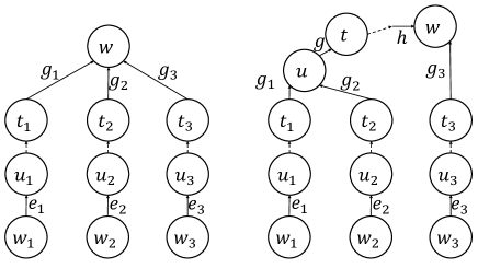
  Figure 2: Two cases for $g_{1},g_{2},g_{3}$. The left figure shows the case when they all meet at the same vertex $w$. The right figure shows when $g_{1}$ and $g_{2}$ meet first at $u$ and meet $g_{3}$ with $w$ later. Real lines indicate an individual arc and dotted lines indicate a directed path.

  First, suppose all $g_{1},g_{2},g_{3}$ meet at the same vertex $w$; in other words, $g_{i}=(t_{i},w)$ for some $t_{i}$’s. Then, by (6), $x_{wg_{i}}>1-\beta-2\varepsilon$ for each $i$. With (5), it implies $\sum_{i}x_{wg_{i}}>3(1-\beta)-6\varepsilon\geq 1$, which violates the constraint (3) of the LP.

  Finally, without loss of generality, suppose $g_{1}$ and $g_{2}$ meet at $u$, which is not incident on $g_{3}$; in other words, $g_{1}=(t_{1},u),g_{2}=(t_{2},u),g_{3}=(t_{3},w)$ for some $t_{i}$’s, where $w$ is an ancestor of $u$ in $\overrightarrow{T}$ and is the first vertex where all $P_{1},P_{2},P_{3}$ intersect. Let $\overrightarrow{T}$ be the parent of $u$ in the tree $\overrightarrow{T}$ ($\overrightarrow{T}$ may be equal to $w$), and $g=(u,t)$. Then, (6), implies $x_{ug_{i}}>1-\beta-2\varepsilon$ for $i\in\{1,2\}$, which, combined with the LP constraint (3) for $u$, yields

  $$x_{ug}<1-2(1-\beta-2\varepsilon)=2\beta-1+4\varepsilon.$$

  Together again with the LP constraint (2) for $g$, we have

  $$x_{tg}>1-x_{ug}-z_{t}>2-2\beta-5\varepsilon.$$

  Let $h$ be the last arc of the path from $u$ to $w$. Using Claim 6 again, we conclude that $x_{wh}>2-2\beta-6\varepsilon$. Combined with $x_{wg_{3}}>1-\beta-2\varepsilon$ and $h$ and $g_{3}$ are different, it implies $x_{wh}+x_{wg_{3}}>3-3\beta-8\varepsilon\geq 1$ by (5), which contradicts the constraint (3) of the LP for $w$. $\blacklozenge$

Now we compute the probability that $v$ is deleted by Step (iii) of the rounding algorithm. It happens whether $v$ itself is directly deleted or some vertex $u\in\textit{anc}(v)=V(\overrightarrow{T})$ is directly deleted by a target $e=(w,u)$. By Claim 7, no three targets are pairwise comparable, and by Dilworth’s Theorem, all targets are contained in two directed paths $P_{1},P_{2}$ in $\overrightarrow{T}$. By the choice of the rounding algorithm, for one path $P_{1}=(u_{0},\dots,u_{k}=v)$, for each $i\in[k]$,

$$\Pr[u_{i}\mbox{ is directly deleted by }(u_{i-1},u_{i})]\leq\frac{y_{(u_{i-1},u_{i})}}{\beta-\alpha}=\frac{z_{u_{i}}-z_{u_{i-1}}}{\beta-\alpha}.$$

Summing over all $i$’s yields

$$\sum_{i=1}^{k}\frac{z_{u_{i}}-z_{u_{i-1}}}{\beta-\alpha}=\frac{z_{u_{k}}-z_{u_{0}}}{\beta-\alpha}\leq\frac{z_{v}}{\beta-\alpha}.$$

We can apply the same analysis to $P_{2}$ and use the union bound. ∎

We now examine structure of the remaining graph after the rounding procedure. We first show that in the original graph, each arc, if not deleted, is pointed to by at least one of its endpoints.

Claim 8.

For each $e=(u,v)\in A$, if neither $u$ nor $v$ was deleted during the rounding, $e$ is pointed to by at least one of them.

• Proof of Claim. Since $v$ is not deleted, it means $z_{v}<\varepsilon$, which, by (2), implies that $x_{ue}+x_{ve}>1-\varepsilon\Leftrightarrow\bar{x}_{ue}+\bar{x}_{ve}<1+\varepsilon$. Since $\theta\geq\alpha$, by (4), either $\theta\geq\bar{x}_{ue}$ or $\theta\geq\bar{x}_{ue}$. $\blacklozenge$

The following lemma shows that after the rounding, each connected component (in the undirected sense) has at most one cycle.

Lemma 4.3.

Let $S$ be the set of vertices deleted during the rounding algorithm. In each connected component of $\mathsf{Und}(\overrightarrow{G}\setminus S)$, there is at most one (undirected) cycle.

Proof.

The proof proceeds by examining how vertices can possibly point to adjacent arcs. First, the following claim shows that one vertex cannot point to more than two arcs.

Claim 9.

Every vertex $v\in V$ points to at most two arcs.

• Proof of Claim. Assume towards contradiction that $v$ points to three arcs $e,f,$ and $g$. It implies $\bar{x}_{ve},\bar{x}_{vf},\bar{x}_{vg}$ are all strictly less than $\theta\leq\beta$, which implies that $x_{ve}+x_{vf}+x_{vg}>3(1-\beta)$. Since $3(1-\beta)\geq 1$ by (5), it contradicts the constraint (3) of the LP relaxation. $\blacklozenge$

Moreover, the following claim constrains the way arcs in a cycle are pointed to by its vertices.

Claim 10.

For every arc $e\in A$, if it is pointed to by exactly one of its endpoint, say $v$, then it is the only arc that $v$ points to.

• Proof of Claim. We first show $\theta<x_{ve}+z_{v}$. If $e=(u,v)$, the assumption that $u$ does not point to $e$ implies

  $$\theta<\bar{x}_{ue}=1-x_{ue}=1-(1-x_{ve}-z_{v})=x_{ve}+z_{v},$$

  where the second equality follows from (2). Even when $e=(v,u)$, the assumption that $e$ is not deleted and $u$ does not point to $e$ implies

  $$\theta<\bar{x}_{ue}-y_{e}=\bar{x}_{ue}-(z_{u}-z_{v})=1-x_{ue}-z_{u}+z_{v}=x_{ve}+z_{v},$$

  where the last equality follows from the constraint (2) of the LP relaxation. Therefore, $\theta<x_{ve}+z_{v}$ in any case.

  If $v$ points to any other arc $f$, it implies

  $$\theta>\bar{x}_{vf}=1-x_{vf}\geq z_{v}+x_{ve},$$

  where the inequality follows from the constraint (3) of the LP relaxation. This leads to contradiction, proving the claim. $\blacklozenge$

Therefore, after the rounding, in the remaining graph $\overrightarrow{G}\setminus S$, (i) every remaining arc is pointed by at least one of its endpoints, (ii) each vertex points to at most two arcs, and (iii) if one vertex does not point to an arc incident on it, the other endpoint uniquely points to the arc.

Consider an undirected cycle $(v_{1},\dots,v_{k},v_{k+1})$ in $\mathsf{Und}(\overrightarrow{G}\setminus S)$ with $v_{1}=v_{k+1}$, so that either $(v_{i},v_{i+1})$ or $(v_{i+1},v_{i})$ is in $A$ for every $i\in[k]$. Let $\{v_{i},v_{i+1}\}$ denotes an undirected edge. If an edge in this cycle is pointed to by only one of its endpoints (without loss of generality, say $\{v_{k},v_{1}\}$ is only pointed to by $v_{1}$), then $v_{1}$ cannot point to any other edge, so $\{v_{2},v_{1}\}$ is uniquely pointed to by $v_{2}$ by (iii), and this inductively leads to every $\{v_{i},v_{i+1}\}$ uniquely pointed to by $v_{i+1}$ for $1\leq i<k$. Note that all $v_{1},\dots,v_{k}$ cannot point to any edge outside the cycle. Even when all edges are pointed to by both endpoints, by (ii), all $v_{1},\dots,v_{k}$ cannot point to any edge outside the cycle.

Assume towards contradiction that there are two undirected cycles $C_{1}$ and $C_{2}$ (not necessarily vertex or edge disjoint) in the same connected component of $\mathsf{Und}(\overrightarrow{G}\setminus S)$. If $V(C_{1})\cap V(C_{2})\neq\emptyset$, there must be a vertex $v\in C_{2}$ that points to an edge in $C_{1}\setminus C_{2}$. This contradicts the above paragraph. If $C_{1}$ and $C_{2}$ are vertex disjoint, let $(v_{1},\dots,v_{k})$ be an undirected path from $C_{1}$ and $C_{2}$ where $v_{1}\in C_{1}$ and $v_{k}\in C_{2}$. By the above paragraph, $\{v_{1},v_{2}\}$ is uniquely pointed to by $v_{2}$ and inductively $\{v_{i},v_{i+1}\}$ is uniquely pointed to by $v_{i+1}$. But applying the same argument from $\{v_{k-1},v_{k}\}$, $\{v_{i},v_{i+1}\}$ must be uniquely pointed to by $v_{i}$, leading to contradiction. Therefore, there must be only one undirected cycle in each connected component. ∎

After the rounding, each connected component has at most one cycle, so we can easily compute the optimal solution efficiently. Therefore, we compute a feasible solution that respects the constraints of the Feedback Vertex Set with Precedence Constraints. Since the total weights of deleted vertices in each step is at most $\mathsf{LP}/\varepsilon$ in Step (i), at most $2\mathsf{LP}/(\beta-\alpha)$ in Step (iii), and at most $\mathsf{OPT}$ in the final cleanup step, the final approximation ratio is

$$\frac{1}{\varepsilon}+\frac{2}{\beta-\alpha}+1\leq 62.2$$

by our choice of $\varepsilon=0.0293258,\alpha=0.514663,\beta=0.588465$.

5 Conclusions

In this paper, we show that Ptolemaic Deletion admits a polynomial-time constant-factor approximation algorithm. To this end, we introduce Feedback Vertex Set with Precedence Constraints, which is a variant of Weighted Feedback Vertex Set with additional constraints including that any solution set must be downward-closed  i.e., if a node being in a solution propels all its descendants in the input (acyclic) digraph to be in the solution. To attain an approximation algorithm for Ptolemaic Deletion from that for Feedback Vertex Set with Precedence Constraints, we investigate the structure of inter-clique digraphs of graphs which give us a tree-like structure when an input graph is ptolemaic and have a laminar structure when an input graph is ($C_{4}$, gem)-free. Feedback Vertex Set with Precedence Constraints can be utilized for wider purposes in other parameterized problems, because through our approximation algorithm, one can find a hereditary feedback vertex set of an input graph, where the hereditary property captures the essence of the parameterized problems.

As the purpose of this paper, for various graph classes $\mathcal{F}$, it would be interesting to investigate whether Weighted $\mathcal{F}$-Deletion admits a constant-factor approximation algorithm; for instance, Chordal Vertex Deletion or $\ell$-Leaf Power Vertex Deletion for $\ell\geq 4$. For a positive integer $\ell$, a graph $G$ is an $\ell$-leaf power if there is a tree $T$ such that $V(G)$ is equal to the set of leaves of $T$ and $v,w\in V(G)$ are adjacent if and only if $d(v,w)\leq\ell$ in $T$. We remark that $3$-Leaf Power Vertex Deletion admits a constant-factor approximation algorithm by a reduction to Weighted Feedback Vertex Set, as Dom, Guo, Hüffner, and Neidermeier [11] did to show the fixed-parameter tractability of $3$-Leaf Power Vertex Deletion.

References

- [1] Akanksha Agrawal, Sudeshna Kolay, Daniel Lokshtanov, and Saket Saurabh, A faster FPT algorithm and a smaller kernel for block graph vertex deletion, LATIN 2016: Theoretical Informatics, Springer, 2016, pp. 1–13.
- [2] Akanksha Agrawal, Daniel Lokshtanov, Pranabendu Misra, Saket Saurabh, and Meirav Zehavi, Feedback vertex set inspired kernel for chordal vertex deletion, ACM Transactions on Algorithms (TALG) 15 (2018), no. 1, 1–28.
- [3] , Polylogarithmic approximation algorithms for weighted-f-deletion problems, Approximation, Randomization, and Combinatorial Optimization. Algorithms and Techniques (APPROX/RANDOM 2018), Schloss Dagstuhl-Leibniz-Zentrum fuer Informatik, 2018.
- [4] Akanksha Agrawal, Pranabendu Misra, Saket Saurabh, and Meirav Zehavi, Interval vertex deletion admits a polynomial kernel, Proceedings of the Thirtieth Annual ACM-SIAM Symposium on Discrete Algorithms, SIAM, 2019, pp. 1711–1730.
- [5] Jungho Ahn, Eduard Eiben, O-joung Kwon, and Sang-il Oum, A polynomial kernel for -leaf power deletion, arXiv:1911.04249, manuscript, 2019.
- [6] Andreas Brandstädt and Van Bang Le, Structure and linear time recognition of 3-leaf powers, Inform. Process. Lett. 98 (2006), no. 4, 133–138. MR 2211095
- [7] Yixin Cao, Linear recognition of almost interval graphs, Proceedings of the twenty-seventh annual ACM-SIAM symposium on Discrete algorithms, SIAM, 2016, pp. 1096–1115.
- [8] Yixin Cao and Dániel Marx, Interval deletion is fixed-parameter tractable, ACM Transactions on Algorithms (TALG) 11 (2015), no. 3, 1–35.
- [9] Yixin Cao and Dániel Marx, Chordal editing is fixed-parameter tractable, Algorithmica 75 (2016), no. 1, 118–137.
- [10] Chandra Chekuri and Vivek Madan, Constant factor approximation for subset feedback set problems via a new lp relaxation, Proceedings of the twenty-seventh annual ACM-SIAM symposium on Discrete algorithms, SIAM, 2016, pp. 808–820.
- [11] Michael Dom, Jiong Guo, Falk Hüffner, and Rolf Niedermeier, Error compensation in leaf power problems, Algorithmica 44 (2006), no. 4, 363–381.
- [12] Eduard Eiben, Robert Ganian, and O-joung Kwon, A single-exponential fixed-parameter algorithm for distance-hereditary vertex deletion, Journal of Computer and System Sciences 97 (2018), 121–146.
- [13] Martin Farber, On diameters and radii of bridged graphs, Discrete Mathematics 73 (1989), no. 3, 249–260.
- [14] Samuel Fiorini, Gwenaël Joret, and Ugo Pietropaoli, Hitting diamonds and growing cacti, International Conference on Integer Programming and Combinatorial Optimization, Springer, 2010, pp. 191–204.
- [15] Fedor V Fomin, Daniel Lokshtanov, Neeldhara Misra, and Saket Saurabh, Planar f-deletion: Approximation, kernelization and optimal FPT algorithms, 2012 IEEE 53rd Annual Symposium on Foundations of Computer Science, IEEE, 2012, pp. 470–479.
- [16] Anupam Gupta, Euiwoong Lee, Jason Li, Pasin Manurangsi, and Michał Włodarczyk, Losing treewidth by separating subsets, Proceedings of the Thirtieth Annual ACM-SIAM Symposium on Discrete Algorithms, SIAM, 2019, pp. 1731–1749.
- [17] Pinar Heggernes, Pim Van’t Hof, Bart MP Jansen, Stefan Kratsch, and Yngve Villanger, Parameterized complexity of vertex deletion into perfect graph classes, International Symposium on Fundamentals of Computation Theory, Springer, 2011, pp. 240–251.
- [18] Edward Howorka, A characterization of Ptolemaic graphs, J. Graph Theory 5 (1981), no. 3, 323–331. MR 625074
- [19] Bart MP Jansen and Marcin Pilipczuk, Approximation and kernelization for chordal vertex deletion, Proceedings of the Twenty-Eighth Annual ACM-SIAM Symposium on Discrete Algorithms, SIAM, 2017, pp. 1399–1418.
- [20] Haim Kaplan, Ron Shamir, and Robert Endre Tarjan, Tractability of parameterized completion problems on chordal and interval graphs: Minimum fill-in and physical mapping, 35th Annual Symposium on Foundations of Computer Science, Santa Fe, New Mexico, USA, 20-22 November 1994, IEEE Computer Society, 1994, pp. 780–791.
- [21] Eun Jung Kim and O-joung Kwon, A polynomial kernel for distance-hereditary vertex deletion, Workshop on Algorithms and Data Structures, Springer, 2017, pp. 509–520.
- [22] , Erdős-Pósa property of chordless cycles and its applications, Proceedings of the Twenty-Ninth Annual ACM-SIAM Symposium on Discrete Algorithms, SIAM, Philadelphia, PA, 2018, pp. 1665–1684. MR 3775897
- [23] Eun Jung Kim, Alexander Langer, Christophe Paul, Felix Reidl, Peter Rossmanith, Ignasi Sau, and Somnath Sikdar, Linear kernels and single-exponential algorithms via protrusion decompositions, ACM Transactions on Algorithms (TALG) 12 (2015), no. 2, 1–41.
- [24] Stefan Kratsch and Magnus Wahlström, Compression via matroids: a randomized polynomial kernel for odd cycle transversal, ACM Transactions on Algorithms (TALG) 10 (2014), no. 4, 1–15.
- [25] Daniel Lokshtanov, Pranabendu Misra, Fahad Panolan, Geevarghese Philip, and Saket Saurabh, A (2 + )-factor approximation algorithm for split vertex deletion, Proceedings of the Forty-Seventh International Colloquium on Automata, Languages and Programming, 2020.
- [26] Dániel Marx, Chordal deletion is fixed-parameter tractable, Algorithmica 57 (2010), no. 4, 747–768.
- [27] Sang-il Oum, Rank-width and vertex-minors, J. Comb. Theory, Ser. B 95 (2005), no. 1, 79–100.
- [28] Bruce Reed, Kaleigh Smith, and Adrian Vetta, Finding odd cycle transversals, Operations Research Letters 32 (2004), no. 4, 299–301.
- [29] Shuji Tsukiyama, Mikio Ide, Hiromu Ariyoshi, and Isao Shirakawa, A new algorithm for generating all the maximal independent sets, SIAM J. Comput. 6 (1977), no. 3, 505–517.
- [30] Ryuhei Uehara and Yushi Uno, Laminar structure of Ptolemaic graphs with applications, Discrete Appl. Math. 157 (2009), no. 7, 1533–1543. MR 2510233
- [31] Mihalis Yannakakis, Computing the minimum fill-in is np-complete, SIAM Journal on Algebraic and Discrete Methods 2 (1981).