Instability of mixing in the Kuramoto model: From bifurcations to patterns

Abstract

We study patterns observed right after the loss of stability of mixing in the Kuramoto model of coupled phase oscillators with random intrinsic frequencies on large graphs, which can also be random. We show that the emergent patterns are formed via two independent mechanisms determined by the shape of the frequency distribution and the limiting structure of the underlying graph sequence. Specifically, we identify two nested eigenvalue problems whose eigenvectors (unstable modes) determine the structure of the nascent patterns. The analysis is illustrated with the results of the numerical experiments with the Kuramoto model with unimodal and bimodal frequency distributions on certain graphs.

1 Introduction

Models of interacting dynamical systems come up in different areas of science and technology. Modern applications ranging from neuroscience to power grids emphasize models with spatially structured interactions defined by graphs. Identifying dynamical mechanisms underlying pattern formation in such networks is an interesting problem with many important applications. In this paper, we study patterns emerging near the loss of stability of mixing in the Kuramoto model (KM) with random intrinsic frequencies on large graphs. We show that by varying the frequency distribution and the graph structure, one can generate a rich variety of spatiotemporal patterns and identify a precise mathematical mechanism underlying pattern formation in this model.

The KM is one of the most widely used models in the theory of synchronization. In this paper, we study the KM on graphs, which is formulated as follows. Let $(\Gamma^{n})$ be a sequence of graphs and consider

$$\dot{\theta}_{i}=\omega_{i}+K(\alpha_{n}n)^{-1}\sum_{j=1}^{n}a^{n}_{ij}\sin(\theta_{j}-\theta_{i}),\quad i\in[n]:=\{1,2,\dots,n\},$$ (1.1)

where $\theta_{i}:{\mathbb{R}}^{+}\to\mathbb{T}:={\mathbb{R}}/2\pi{\mathbb{Z}}$ stands for the phase of oscillator $i$; $\omega_{i},i\in[n],$ are independent random intrinsic frequencies drawn from the distribution with density $g(\omega),$ and $K$ is the strength of coupling. $(a^{n}_{ij})$ is an $n\times n$ symmetric (weighted) adjacency matrix of graph $\Gamma^{n}$. The scaling sequence $\alpha_{n}$ is either identically equal to $1$ if $(\Gamma^{n})$ is a sequence of dense graphs, or $\alpha_{n}\searrow 0$ subject to condition $n\alpha_{n}\rightarrow\infty$ if $(\Gamma^{n})$ is a sequence of sparse graphs with edge density $O(n\alpha_{n})$. For more details on the KM on sparse graphs we refer an interested reader to [15].

Suppose $(\Gamma^{n})$ is a convergent sequence of graphs whose limiting behavior is described by a symmetric graphon $W\in L^{2}([0,1]^{2})$ (cf. [15]). Then under fairly general assumptions, the dynamics of (1.1) for large $n$ can be approximated by the Vlasov equation

$$\partial_{t}f(t,\theta,\omega,x)+\partial_{\theta}\left\{V(t,\theta,\omega,x)f(t,\theta,\omega,x)\right\}=0,$$ (1.2)

where $f(t,\theta,\omega,x)$ is a probability density function in $(\theta,\omega)\in\mathbb{T}\times{\mathbb{R}}$ of an oscillator at point $x\in I:=[0,1]$ at time $t\in{\mathbb{R}}^{+}$. The velocity field is defined as follows

$$V(t,\theta,\omega,x)=\omega+{K\over 2{i\mkern 1.0mu}}\left(\kappa(t,x)e^{-{i\mkern 1.0mu}\theta}-\overline{\kappa(t,x)e^{-{i\mkern 1.0mu}\theta}}\right),$$ (1.3)

where

$$\kappa(t,x)=\int_{\mathbb{T}}e^{i\theta}\int_{\mathbb{R}}\left(\boldsymbol{W}f(t,\theta,\omega,\cdot)\right)(x)d\omega d\theta,$$ (1.4)

is called a (local) order parameter. The following self-adjoint compact operator on $L^{2}([0,1])$ will play an important role

$$\left(\boldsymbol{W}\phi\right)(x):=\int_{I}W(x,y)\phi(y)dy,\quad I:=[0,1].$$ (1.5)

Rigorous justification of the Vlasov equation (1.2) in the context of the KM with all–to–all coupling was given in [14]. It is based on the classical theory for kinetic equations (cf.  [16, 1, 9]). For the KM on dense graphs, the Vlasov equation was further justified in [12, 4]. For the KM on sparse graphs with unbounded degree, the results in [12, 4] continue to hold when combined with [15, Theorem 4.1].

Equation (1.2) has a steady state solution

$$f_{mix}={g(\omega)\over 2\pi}.$$ (1.6)

It describes the regime when all phases are uniformly distributed over $\mathbb{T}$, which corresponds to mixing. Numerical experiments show that mixing is stable for small $|K|$. In his classical work on synchronization, Kuramoto identified the critical value $K_{c}=2\left(\pi g(0)\right)^{-1}$ marking the loss of stability of mixing [13]. This formula assumes all–to–all coupling (i.e., $W\equiv 1$) and continuous even unimodal density $g(\omega)$. Kuramoto’s findings started a new area of research, which culminated in a rigorous analysis of the loss of stability of mixing in the KM with all–to–all coupling in [2]. For the KM on graphs, bifurcations of the mixing state were analyzed in [4, 5]. Interestingly, the analysis of the spatially extended model along with the pitchfork bifurcation at positive value of $K$ leading to synchronization reveals the possibility of a bifurcation for $K<0$. For instance, it was shown that for a network with nonlocal nearest-neighbor coupling there is a bifurcation to so–called twisted states at a certain $K^{-}_{c}<0$ [5, 7]. Thus, network structure plays a role in the loss of stability of mixing and affects the emerging patterns.

From the beginning, the studies of the KM have been mainly focused on the transition to synchronization, i.e., on the pitchfork bifurcation of mixing. This turned out to be a challenging problem. The main technical obstacle to the bifurcation analysis was the presence of continuous spectrum on the imaginary axis. It was overcome in [2] with the help of the generalized spectral theory. The method of [2] was further applied to the analysis of Andronov–Hopf bifurcation in [3] and was extended to the KM on graphs in [4, 5]. The technical difficulty of the bifurcation analysis for a long time obstructed its pattern formation aspect, which is perhaps even more interesting from the nonlinear science point of view. The examples in [7] already give a glimpse into pattern formation capacity of spatially extended KM. In this note, we develop this theme further. We show that the combination of frequency distribution and graph structure provides a flexible mechanism for controlling spatiotemporal patterns arising at the loss of stability of mixing in the KM on graphs. Surprisingly, the contributions of the frequency distribution and the graph structure are independent from each other, which results in a variety of possible patterns obtained by combining features controlled by these two (vector–valued) parameters (Figures 2-5). Furthermore, we show that asymmetric frequency distribution results in asymmetric chimera like patterns (Figure 7). To keep the presentation simple, we restrict to linear stability analysis, which is sufficient to relate bifurcations to patterns. Readers interested in the analysis beyond linear stability are referred to [5] for the treatment of the pitchfork bifurcation in the KM on graphs. The Andronov–Hopf bifurcation is analyzed similarly by extending the results in [3] to the spatially extended model following the lines of [5].

The outline of the paper is as follows. In the next section, we perform a linear stability analysis of mixing. This is done for completeness, as the stability of mixing in the KM on graphs was already analyzed in [4, 5]. To complement the presentation in [4], this time we adapt the approach based on the theory for Volterra equations from [8] to the KM on graphs. It affords a quick derivation of the equation for the critical values of $K$ and provides a nice geometric picture of the loss of stability of mixing in the KM. After locating the instabilities, we compute the unstable modes, which determine the bifurcating patterns. As shown in [4] the loss of stability in the KM on graphs is captured by two nested eigenvalue problems. The first one is obtained via the Fourier transform of the linearized system and is the same as in the stability analysis of the KM with all–to–all coupling [2, 8]. We refer to this problem as the principal problem. The second one is that for $\boldsymbol{W}$ (cf. (1.5)) and is called a secondary eigenvalue problem. It turns out that each problem is responsible for specific features of the bifurcating solutions: the principal modes determine the local structure of the emerging patterns, whereas the secondary modes capture their spatial organization. In particular, the principal eigenvalue problem determines whether mixing loses stability via a pitchfork or an Andronov–Hopf bifurcation. The former results in stationary patterns, whereas the latter produces patterns traveling with a nonzero speed. However, it is the secondary eigenvalue problem that decides the actual pattern. Depending on the form of the eigenfunctions corresponding to the critical eigenvalue of the secondary problem, one can observe spatially uniform clusters or patterns with more complex spatial organization like twisted states. Importantly, the two spectral problems are independent in the sense that one is determined by the shape of the frequency distribution while the other - by the graph structure. After deriving the necessary analytical tools in Section 2, we turn to the detailed discussion of the bifurcating patterns in the KM with unimodal and bimodal $g$ in Section 3. To this end, we compare solutions bifurcating from the mixing state in the KM on all–to–all and nonlocal nearest–neighbor graphs. These examples clearly demonstrate the contributions of the principal and secondary unstable modes to the structure of the emerging patterns.

2 Linear stability

In this section, we rewrite (1.2) in Fourier variables and linearize the resultant system about the mixing steady state. Then we reduce the problem of stability to the Volterra equation for vector–valued functions and derive the equation for the eigenvalues of the linearized operator. Here, we extend the method in [8] to the KM on graphs. Then we compute the corresponding eigenvalues following [5]. This information is sufficient to explain the patterns emerging at the loss of stability of mixing, which is the main focus of this paper. For more details on stability analysis of mixing in the KM on graphs, we refer an interested reader to [4, 5].

We start by applying the Fourier transform in $(\theta,\omega)$

$$u(t,l,\xi,x)=\int_{\mathbb{T}}\int_{\mathbb{R}}e^{{i\mkern 1.0mu}l\theta}e^{{i\mkern 1.0mu}\xi\omega}f(t,\theta,\omega,x)d\omega d\theta,\quad(l,\xi,x)\in{\mathbb{Z}}\times{\mathbb{R}}\times I$$ (2.1)

to (1.2). Note that by the definition of $f,$

$$g(\omega)=\int_{\mathbb{T}}f(t,\theta,\omega,x)d\theta\quad\forall(x,t)\in I\times{\mathbb{R}}^{+}.$$ (2.2)

Thus, by Fubini’s theorem,

$$u(t,0,\xi,x)=\int_{\mathbb{R}}e^{{i\mkern 1.0mu}\xi\omega}g(\omega)d\omega=:(\mathcal{F}g)(\xi),$$ (2.3)

where $\mathcal{F}g$ stands for the Fourier transform in $\omega$ throughout this paper.

Following [8], we assume

$$\mathcal{F}g\in C_{a}({\mathbb{R}})=\{\phi\in C({\mathbb{R}}):\;\|\phi\|_{a}=\sup_{t\in{\mathbb{R}}}e^{at}|\phi(t)|<\infty\}\;\mbox{for some}\;a>0.$$ (2.4)

Further, since $f$ is real, $\overline{u(t,l,\xi,x)}=u(t,-l,-\xi,x)$ it is sufficient to consider

$$\partial_{t}u(t,1,\xi,x) = \partial_{\xi}u(t,1,\xi,x)+{K\over 2}\left(\kappa(t,x)(\mathcal{F}g)(\xi)-\overline{\kappa(t,x)}u(t,2,\xi,x)\right),$$ (2.5)

$$\partial_{t}u(t,l,\xi,x) = l\partial_{\xi}u(t,l,\xi,x)+{Kl\over 2}\left(\kappa(t,x)u(t,l-1,\xi,x)-\overline{\kappa(t,x)}u(t,l+1,\xi,x)\right),$$ (2.6)

for $\geq 2$. Note that $\kappa$ defined in (1.4) can be rewritten as

$$\kappa(t,x)=\int_{I}W(x,y)u(t,1,0,y)dy.$$ (2.7)

The equilibrium $f_{mix}$ corresponds to $u_{mix}=(\mathcal{F}g,0,0,\dots)$ in the Fourier space for $l\in\{0,1,2,\dots\}$. The linearization of about $u_{mix}$ is thus given by

$$\partial_{t}u(t,1,\xi,x) = \partial_{\xi}u(t,1,\xi,x)+{K\over 2}\kappa(t,x)(\mathcal{F}g)(\xi),$$ (2.8)

$$\partial_{t}u(t,l,\xi,x) = l\partial_{\xi}u(t,l,\xi,x),\;l\geq 2.$$ (2.9)

Equations in (2.9) describe pure transport. Thus, stability is decided by (2.8), which we rewrite as

$$\partial_{t}\phi=\boldsymbol{T}\phi.$$ (2.10)

$\boldsymbol{T}$ is viewed as a linear operator densely defined on $L^{2}\left([0,1];C_{a}({\mathbb{R}})\right).$

Integrating (2.8) along characteristics and recalling (2.7), we have

$$u(t,1,\xi,x)=u_{0}(1,\xi+t,x)+{K\over 2}\int_{0}^{t}\left(\boldsymbol{W}u(s,1,0,\cdot)\right)(\mathcal{F}g)(\xi+(t-s))ds,$$ (2.11)

By plugging $\xi=0$ in (2.11), we obtain the following Volterra equation

$$u(t,x)=u_{0}(t,x)+{K\over 2}\int_{0}^{t}\left(\boldsymbol{W}u(s,\cdot)\right)(\mathcal{F}g)(t-s)ds,$$ (2.12)

where by abuse of notation $u(t,x):=u(t,1,0,x)$. We recast (2.12) in a more general form

$$\boldsymbol{\nu}(t)+\int_{0}^{t}\boldsymbol{A}(t-s)\boldsymbol{\nu}(s)ds=\boldsymbol{\phi}(t),$$ (2.13)

where $\boldsymbol{A}:{\mathbb{R}}^{+}\to L(\mathcal{H})$ and $\boldsymbol{\phi},\boldsymbol{\nu}:{\mathbb{R}}\to\mathcal{H}$. By $L(\mathcal{H})$ we denote the space of linear bounded operators on $\mathcal{H}$. For the problem at hand, $\mathcal{H}=L^{2}([0,1])$,

$$\boldsymbol{A}(t)={-K\over 2}(\mathcal{F}g)(t)\boldsymbol{W}\quad\mbox{and}\quad\boldsymbol{\phi}(t)=u_{0}(t,\cdot),\;\boldsymbol{\nu}(t)=u(t,\cdot).$$ (2.14)

From now on, we will use the bold font to denote vector–valued functions along with operators.

Theorem 2.1.

[11, Theorems 1 & 2] Let $\boldsymbol{A}:{\mathbb{R}}^{+}\to L(\mathcal{H})$ be strongly measurable and $\|\boldsymbol{A}(\cdot)\|\in L^{1}_{loc}({\mathbb{R}}^{+};{\mathbb{R}}),$ where $\|\cdot\|$ stands for the operator norm. Then there exists a strongly measurable resolvent $\operatorname{\mathbf{R}}:{\mathbb{R}}^{+}\to L(\mathcal{H})$

$$\operatorname{\mathbf{R}}(t)=\boldsymbol{A}(t)-\int_{0}^{t}\operatorname{\mathbf{R}}(t-s)\boldsymbol{A}(s)ds=\boldsymbol{A}(t)-\int_{0}^{t}\boldsymbol{A}(t-s)\operatorname{\mathbf{R}}(s)ds.$$ (2.15)

For any $\boldsymbol{\phi}\in L^{1}_{loc}({\mathbb{R}}^{+},\mathcal{H})$ the unique solution of (2.13) can be expressed as

$$\boldsymbol{\nu}(t)=\boldsymbol{\phi}(t)-\int_{0}^{t}\operatorname{\mathbf{R}}(t-s)\boldsymbol{\phi}(s)ds.$$ (2.16)

Moreover, $\operatorname{\mathbf{R}}\in L^{1}({\mathbb{R}}^{+};L(\mathcal{H}))$ if and only if $\mathbf{I}+(\mathcal{L}\boldsymbol{A})(z)$ is invertible as a bounded operator on $\mathcal{H}$ for all $z\in{\mathbb{C}}$ with $\Re z\geq 0$. Here,

$$\mathcal{L}\boldsymbol{A}(z)=\int_{0}^{t}e^{-zt}\boldsymbol{A}(t)dt.$$ (2.17)

Remark 2.2.

For (2.12) following the lines of the analysis in the finite–dimensional case [10, Theorem 3.1], the resolvent can be obtained constructively as a Neumann series

$$\operatorname{\mathbf{R}}{\mathbf{h}}=-\sum_{j=1}^{\infty}{k^{\ast}}^{j}\ast(\boldsymbol{W}^{j}\mathbf{h}),\quad k(t)={K\over 2}(\mathcal{F}g)(t),$$

or in expanded form

$$(\operatorname{\mathbf{R}}h)(t,x)=-\sum_{j=1}^{\infty}\int_{0}^{t}{(k^{\ast}}^{j}(t-s)\left(\boldsymbol{W}^{j}h(s,\cdot)\right)(x)ds.$$

Here, $k\ast a$ stands for the convolution of two functions $(k\ast a)(t)=\int_{0}^{t}k(t-s)a(s)ds$. Similarly,

$${k^{\ast}}^{j}\ast a=\underbrace{k\ast(k\ast\dots\ast(k\ast}_{j\,\mbox{times}}a)\dots).$$

The data in (2.12) clearly satisfy the assumptions of Theorem 2.1. Our next goal is to understand invert-ability of $\boldsymbol{M}(z)=\mathbf{I}+(\mathcal{L}\boldsymbol{A})(z)$. By (2.14), $\boldsymbol{M}(z)$ is invertible unless $z$ is a root of

$$G(z)={2\over K\mu},\;G(z):=\mathcal{L}\left(\mathcal{F}g\right)(z),\quad\mu\in\operatorname{Spec}(\boldsymbol{W})/\{0\}.$$ (2.18)

Below, we will need the following observation

$$G(z)=\int_{0}^{\infty}(\mathcal{F}g)(t)e^{-tz}dt=\int_{0}^{\infty}\int_{-\infty}^{\infty}e^{{i\mkern 1.0mu}(\xi+t)\eta}e^{-tz}g(\eta)d\eta dt=\int_{-\infty}^{\infty}{g(\eta)\over z-{i\mkern 1.0mu}\eta}d\eta,$$ (2.19)

where we used Fubini’s theorem.

Equation (2.18) will be used to compute the eigenvalues of $\boldsymbol{T}$. The corresponding eigenfunctions can be found by extending the corresponding results of the theory for Volterra equations on a finite–dimensional space (cf. [10, Theorem 2.1]) to the problem at hand. For simplicity of presentation, we will compute the eigenfunctions directly using the results in [4].

Let $z=\lambda$ be a root of (2.18) corresponding to $\mu\in\operatorname{Spec}(\boldsymbol{W})$. By Lemma 3.2 in [4] (see also [8, Lemma 27]), $\lambda$ is an eigenvalue of $\boldsymbol{T}$. The corresponding eigenfunction is

$$w_{\lambda}=\mathcal{F}v_{\lambda},$$ (2.20)

where

$$v_{\lambda}(\omega,x)={K\over 2}{g(\omega)\over\lambda-{i\mkern 1.0mu}\omega}\int_{I\times{\mathbb{R}}}W(x,y)v(\lambda,y)dyd\lambda.$$ (2.21)

By integrating both sides of (2.21) with respect to $\omega,$ we have

$$V={K\over 2}G(\lambda)\boldsymbol{W}V,$$

where we used (2.19). $V(x)=\int_{\mathbb{R}}v(\lambda,x)d\lambda$ is an eigenfunction of $\boldsymbol{W}$ corresponding to

$$\mu={K\over 2}G(\lambda).$$

We conclude that

$$w_{\lambda}(\eta,x)=\int_{\mathbb{R}}{e^{{i\mkern 1.0mu}\eta\omega}g(\omega)\over\lambda-{i\mkern 1.0mu}\omega}d\omega\;V(x)$$ (2.22)

is an eigenfunction of $\boldsymbol{T}$ corresponding to eigenvalue $\lambda$. Here, we dropped the factor $K\mu/2$ since eigenfunctions are defined up to a multiplicative constant.

Thus,

$$v_{\lambda}(\omega,x)=\left(\mathcal{F}^{-1}w_{\lambda}(\cdot,x)\right)(\omega)=\Upsilon_{\lambda}(\omega)V(x),\quad\Upsilon_{\lambda}(\omega):={g(\omega)\over\lambda-{i\mkern 1.0mu}\omega}.$$ (2.23)

Remark 2.3.

The separable structure of $v_{\lambda}$ has important implications for pattern formation. $\Upsilon$ and $V$ are determined by the intrinsic frequency distribution $g$ and the graph limit $W$ respectively. Equation (2.23) shows that the frequency distribution and the graph structure shape the unstable modes independently from each other.

Below we will need to know the structure of

$$\Upsilon_{0}=\lim_{\lambda\to 0+0}\Upsilon_{\lambda}=\lim_{\lambda\to 0+0}{g(\omega)\over\lambda-{i\mkern 1.0mu}\omega}.$$

For $(\mathcal{F}g)\in C_{a}({\mathbb{R}})$, $\Upsilon_{0}$ can be viewed as a tempered distribution. Indeed, for any $\phi$ from the Schwartz space $\mathcal{S}({\mathbb{R}})$, by Sokhotski–Plemelj formula (cf. [17]), we have

$$\langle\Upsilon_{0},\phi\rangle=\lim_{\lambda\to 0+0}\int_{-\infty}^{\infty}{g(\omega)\phi(\omega)\over\lambda-{i\mkern 1.0mu}\omega}d\omega=\pi g(0)-{i\mkern 1.0mu}\operatorname{P.V.}\int_{-\infty}^{\infty}{g(\omega)\over\omega}d\omega.$$

Thus, as an element of $\mathcal{S}^{\prime}({\mathbb{R}})$, $\Upsilon_{0}$ can be written as

$$\Upsilon_{0}=\pi g(0)\delta-{i\mkern 1.0mu}\mathcal{P}_{g,0},$$ (2.24)

where $\delta$ stands for the delta function and

$$\langle\mathcal{P}_{g,\alpha},\phi\rangle=\operatorname{P.V.}\int_{-\infty}^{\infty}{g(\omega+\alpha)\phi(\omega+\alpha)\over\omega}d\omega.$$

Similarly, we compute

$$\Upsilon_{\pm{i\mkern 1.0mu}y^{\ast}}:=\lim_{\lambda(0+0)\pm{i\mkern 1.0mu}y^{\ast}}{g(\omega)\over\lambda-{i\mkern 1.0mu}\omega}=\pi g(\pm y^{\ast})\delta_{\pm y^{\ast}}-{i\mkern 1.0mu}\mathcal{P}_{g,\pm y^{\ast}},$$ (2.25)

where $\delta_{\beta}=\delta(\cdot+\beta).$

3 Bifurcations and patterns

Next we turn to the bifurcations in the KM (1.1) and the corresponding patterns. To illustrate the typical scenarios realized in this model we will consider unimodal (U) and bimodal (B) $g\in C_{a}({\mathbb{R}})$ combined with all–to-all (aa) and nonlocal nearest-neighbor connectivity (nn). We will code the corresponding models by (Xy) where $\mbox{\bf X}\in\{\mbox{\bf U},\mbox{\bf B}\}$ and $\mbox{\bf y}\in\{\mbox{\bf aa},\mbox{\bf nn}\}$.

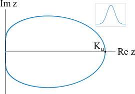
a     b 

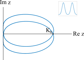
Figure 1: The critical curves generated by a unimodal (a) and bimodal (b) intrinsic frequency distribution.

As a first step, we locate the bifurcations in (1.1) by solving (2.18). To this end, recall (2.19) and note that $G$ is analytic in $\Pi:=\{z\in{\mathbb{C}}:\;\Re z>0\}$ and is continuous in $\bar{\Pi}.$ By Sokhotski–Plemelj formula,

$$\lim_{y\to\pm\infty}\lim_{x\to 0+0}G(x+{i\mkern 1.0mu}y)=\lim_{y\to\pm\infty}\left(\pi g(y)-{i\mkern 1.0mu}\operatorname{P.V.}\int_{-\infty}^{\infty}{g(s)ds\over y-s}\right)=0.$$ (3.1)

Thus, $G$ maps the imaginary axis to a bounded closed curve. As in [8], we use the Argument Principle [17] to conclude that (2.18) has a root in $\Pi$ if and only if

$$2(K\mu)^{-1}\in G(\Pi).$$ (3.2)

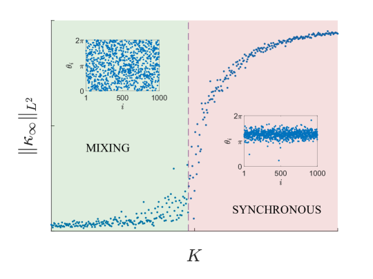
Figure 2: The pitchfork bifurcation leading to the formation of spatially homogeneous synchronous solution in the KM with all–to–all coupling and unimodal $g$. $\kappa_{\infty}$ stands for the time asymptotic value of the $L^{2}$–norm of the local order parameter (1.4). The data presented in this plot was obtained after a long transient time. Further, the $L^{2}$–norm of the local order parameter was averaged over a certain time interval to smoothen the data. The same method was used in all subsequent computations of the order parameter.

In Figure 1, we plot $G(\partial\Pi)$ for symmetric unimodal and bimodal $g$. The critical curve $G(\partial\Pi)$ always intersects the real axis at the origin (cf. (3.1)). In addition, it has another point of intersection with the real axis at

$$K_{u}=G(0)>0,$$ (3.3)

if $g$ is unimodal. In the bimodal case, there is a point of double intersection

$$K_{b}=G(\pm{i\mkern 1.0mu}y^{\ast})>0.$$ (3.4)

Having understood the qualitative features of the critical curves for the unimodal and bimodal densities, we now turn to bifurcations.

(Uaa)

We start with the all–to–all coupling first. In this case, $W\equiv 1$, the largest eigenvalue of $\boldsymbol{W}$ is $\mu=1,$ and the corresponding eigenfunction is constant [4]. Since the critical curve $G(\partial\Pi)$ is bounded, $2K^{-1}\notin\Pi$ for $K\gg 1$. Thus, there are no roots of (2.18) for large $K$. As we decrease $K$, $2K^{-1}$ hits $G(\partial\Pi)$ when

$$2K^{-1}=G(0)=\pi g(0).$$

Note that the corresponding root of (2.18) is $z=0$. Thus, at $K_{c}=2/(\pi g(0))$ the system undergoes a pitchfork bifurcation. The emerging pattern is determined by the unstable mode $v_{0}$, which has a singularity at $\omega=0$. This implies that the emerging pattern contains a stationary cluster. Further, since $V\equiv 1$, the bifurcating solution is uniform in space. We conclude that the instability leads to the formation of a stationary coherent cluster (see Figure 2). This is a classical scenario of the onset of synchronization.

(Baa)

Next we discuss the case of the bimodal density and all–to–all coupling. In this case $2K^{-1}$ hits $G(\partial\Pi)$ at the point of double intersection of the critical curve with the real axis:

$$2K^{-1}=G(0)=\pi g(\pm y^{\ast}).$$

The roots of (2.18) $z=\pm{i\mkern 1.0mu}y^{\ast}$. The system undergoes Andronov–Hopf bifurcation at $K_{c}=1/\left(\pi g(y^{\ast})\right)$ The eigenfunctions $v_{\pm{i\mkern 1.0mu}y^{\ast}}$ have singularities at $\omega=\pm y^{\ast}$ respectively (cf. (2.25)), while $V$ is still constant. Thus, the emerging pattern consists of two spatially homogeneous clusters rotating with constant speed in opposite directions (see Figure 3).

(Unn)

It remains to consider the nonlocal nearest–neighbor coupling (see [4, §5.2] for the definition of $W$ in this case). The new feature here is that along with the largest positive eigenvalue $\mu^{+}=1$ (corresponding to $V^{+}\equiv 1$), there can be one or more negative eigenvalues (see [4] for a detailed discussion). Suppose $\mu^{-}<0$ is the smallest negative eigenvalue of $\boldsymbol{W}$. The corresponding eigenspace is spanned by $V^{-}_{1,2}=e^{\pm 2\pi{i\mkern 1.0mu}qx}$ for some $q\in{\mathbb{N}}$. Thus, there are two bifurcation points

$$K^{+}_{c}=2/(\pi\mu^{+}g(y^{\ast}))>0\quad\mbox{and}\quad K^{-}_{c}=2/(\pi\mu^{-}g(0))<0.$$

$\Upsilon_{0}$ component of the unstable mode $v_{0}$ is the same for the bifurcations at $K_{c}^{-}$ and $K_{c}^{+}$. This implies that the bifurcating patterns gravitate towards stationary clusters. However, the spatial organization is different. The pattern emerging at $K_{c}^{+}$ is uniform in space, whereas those emerging at $K_{c}^{-}$ are organized as $q$–twisted states (see Figure 4).

A new feature of this example is that in addition to positive eigenvalues of $\boldsymbol{W}$ there are negative eigenvalues. Denoting the largest postive and smallest negative eigenvalues of $\boldsymbol{W}$ by $\mu^{+}$ and $\mu^{-}<0$ respectively (see [4] for explicit formulae of the eigenvalues of $\boldsymbol{W}$). For $\mu^{+}$ the corresponding eigenfunction is constant as in the all–to–all coupling case. For $\mu^{-}$, the eigenfunctions are linear combinations of so–called $q$–twisted states: $e^{\pm 2\pi{i\mkern 1.0mu}qx}$ for the appropriare $q\in{\mathbb{N}}$. Thus, in the unimodal case the mixing state bifurcates into a spatially homogeneous solutions at $K^{+}=2/(\pi\mu^{+}g(0))>0$ and into a twisted state at $K^{-}=2/(\pi\mu^{-}g(0))<0$ (see Figure 4). In the bimodal case, the mixing state bifurcates into a two-cluster at $K^{+}=2/(\pi\mu^{+}g(y^{\ast}))>0$ and into a pair of twisted states at $K^{-}=2/(\pi\mu^{-}g(y^{\ast}))<0$ (see Figure 4).

(Bnn)

The only difference of this case with the one that we just discussed is that the principal unstable modes $v_{\pm{i\mkern 1.0mu}y^{\ast}}$ are localized around $\omega=\pm y^{\ast}$. Thus, the stationary patterns in (Unn) turn into rotating ones: rotating clusters at $K_{c}^{+}$ and twisted states traveling in opposite directions at $K_{c}^{-}$ (see Figure 5).

This concludes the description of the bifurcation scenarios in the KM with symmetric unimodal and bimodal frequency distribution on complete and nonlocal nearest–neighbor graphs. Breaking the symmetry of the distribution (see Figure 6) results in new patterns including chimera like patterns shown in Figure 7. They can be understood using the techniques of this paper. The situation is even more interesting for the second–order KM, which will be covered in the future work [6]. The complete and nonlocal nearest–neighbor graphs were used in this paper as representative examples. The analysis of this paper applies without any changes to the KM on a variety of convergent graph sequences including Erdős–Rényi, small-world, and power–law graphs (cf. [7, 15]).

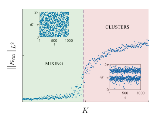
Figure 3: Andronov–Hopf bifurcation leading to the formation of two–cluster in the KM on complete graphs and bimodal $g$.

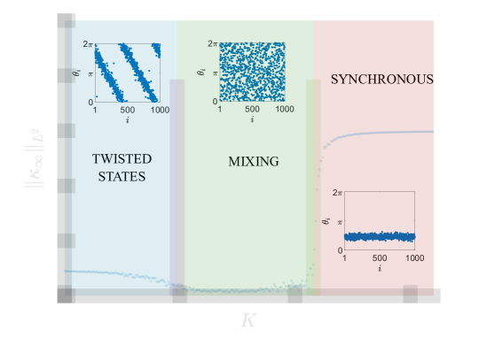
Figure 4: Bifurcations in the KM with nonlocal nearest–neighbor coupling and unimodal frequency distribution. The pitchfork bifurcation at $K_{c}^{-}<0$ leads to formation of a 2–twisted state. At $K_{c}^{+}>0$ the system undergoes a bifurcation leading to synchronization.

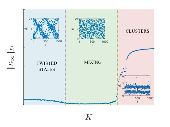
Figure 5: Bifurcations in the KM with nonlocal nearest–neighbor coupling and bimodal frequency distribution. The Andronov–Hopf bifurcation at $K_{c}^{+}>0$ leads to formation of 2–cluster, whereas the bifurcation at $K_{c}^{-}<0$ results in a pair of 2–twisted states traveling in opposite directions.

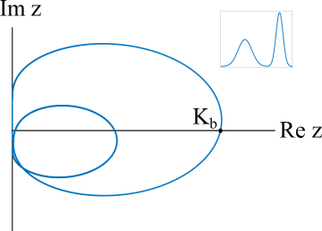
Figure 6: The critical curve for asymmetric bimodal distribution.

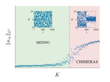
a   b 

Figure 7: The bifurcation diagrams for the KM with asymmetric bimodal distribution (see Figure 6). The coupling is all–to–all in a and nonlocal nearest–neighbor in b. To elucidate the structure of these patterns, we separated the oscillators into two groups depending on the sign of the intrinsic frequency.

Acknowledgements. This work was supported in part by NSF grants DMS 1715161 and 2009233 (to GSM). Numerical simulations were completed using the high performance computing cluster (ELSA) at the School of Science, The College of New Jersey. Funding of ELSA is provided in part by National Science Foundation OAC-1828163. MSM was additionally endorsed by a Support of Scholarly Activities Grant at The College of New Jersey.

References

- [1] W. Braun and K. Hepp, The Vlasov dynamics and its fluctuations in the limit of interacting classical particles, Comm. Math. Phys. 56 (1977), no. 2, 101–113.
- [2] Hayato Chiba, A proof of the Kuramoto conjecture for a bifurcation structure of the infinite-dimensional Kuramoto model, Ergodic Theory Dynam. Systems 35 (2015), no. 3, 762–834.
- [3] Hayato Chiba, A Hopf bifurcation in the Kuramoto-Daido model, arXiv e-prints (2016), arXiv:1610.02834.
- [4] Hayato Chiba and Georgi S. Medvedev, The mean field analysis of the Kuramoto model on graphs I. The mean field equation and transition point formulas, Discrete Contin. Dyn. Syst. 39 (2019), no. 1, 131–155.
- [5] , The mean field analysis of the Kuramoto model on graphs II. Asymptotic stability of the incoherent state, center manifold reduction, and bifurcations, Discrete Contin. Dyn. Syst. 39 (2019), no. 7, 3897–3921.
- [6] Hayato Chiba, Georgi S. Medvedev, and Matthew S. Mizuhara, in preparation.
- [7] , Bifurcations in the Kuramoto model on graphs, Chaos 28 (2018), no. 7, 073109, 10. MR 3833337
- [8] Helge Dietert, Stability and bifurcation for the Kuramoto model, J. Math. Pures Appl. (9) 105 (2016), no. 4, 451–489.
- [9] R. L. Dobrušin, Vlasov equations, Funktsional. Anal. i Prilozhen. 13 (1979), no. 2, 48–58, 96.
- [10] G. Gripenberg, S.-O. Londen, and O. Staffans, Volterra integral and functional equations, Encyclopedia of Mathematics and its Applications, vol. 34, Cambridge University Press, Cambridge, 1990.
- [11] Gustaf Gripenberg, Asymptotic behaviour of resolvents of abstract Volterra equations, J. Math. Anal. Appl. 122 (1987), no. 2, 427–438.
- [12] Dmitry Kaliuzhnyi-Verbovetskyi and Georgi S. Medvedev, The mean field equation for the kuramoto model on graph sequences with non-lipschitz limit, SIAM Journal on Mathematical Analysis 50 (2018), no. 3, 2441–2465.
- [13] Y. Kuramoto, Cooperative dynamics of oscillator community, Progress of Theor. Physics Supplement (1984), 223–240.
- [14] C. Lancellotti, On the Vlasov limit for systems of nonlinearly coupled oscillators without noise, Transport Theory Statist. Phys. 34 (2005), no. 7, 523–535. MR 2265477 (2007f:82098)
- [15] Georgi S. Medvedev, The continuum limit of the Kuramoto model on sparse random graphs, Commun. Math. Sci. 17 (2019), no. 4, 883–898.
- [16] H. Neunzert, Mathematical investigations on particle - in - cell methods, vol. 9, 1978, pp. 229–254.
- [17] Barry Simon, Basic complex analysis, A Comprehensive Course in Analysis, Part 2A, American Mathematical Society, Providence, RI, 2015.